Download as PDF, PPTX
![Graph Models
Class Algorithmic Methods of Data Mining
Program M. Sc. Data Science
University Sapienza University of Rome
Semester Fall 2015
Lecturer Carlos Castillo http://chato.cl/
Sources:
● Frieze, Gionis, Tsourakakis: “Algorithmic techniques for modeling
and mining large graphs (AMAzING)” [Tutorial]
● Lada Adamic: Zipf, Power-Laws and Pareto [Tutorial]
● Giorgios Cheliotis: Social Network Analysis [Tutorial]](https://image.slidesharecdn.com/6qfb9tczqegev93zz5tu-signature-174179124c8bf94a633d0f75ae58d0985739d29f77acf7ddb862c471a419c3cd-poli-151222094555/85/Graph-Evolution-Models-1-320.jpg)
![Graph Models
Class Algorithmic Methods of Data Mining
Program M. Sc. Data Science
University Sapienza University of Rome
Semester Fall 2015
Lecturer Carlos Castillo http://chato.cl/
Sources:
● Frieze, Gionis, Tsourakakis: “Algorithmic techniques for modeling
and mining large graphs (AMAzING)” [Tutorial]
● Lada Adamic: Zipf, Power-Laws and Pareto [Tutorial]
● Giorgios Cheliotis: Social Network Analysis [Tutorial]](https://image.slidesharecdn.com/6qfb9tczqegev93zz5tu-signature-174179124c8bf94a633d0f75ae58d0985739d29f77acf7ddb862c471a419c3cd-poli-151222094555/75/Graph-Evolution-Models-1-2048.jpg)


![18
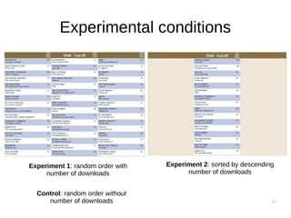
An experiment
● Matthew J. Salganik, Peter Sheridan Dodds,
Duncan J. Watts: Experimental Study of
Inequality and Unpredictability in an Artificial
Cultural Market. Science 10 February 2006.
Vol. 311 no. 5762 pp. 854-856 [link]](https://image.slidesharecdn.com/6qfb9tczqegev93zz5tu-signature-174179124c8bf94a633d0f75ae58d0985739d29f77acf7ddb862c471a419c3cd-poli-151222094555/85/Graph-Evolution-Models-18-320.jpg)
![23
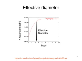
Ways to characterize diameter
● diameter: largest shortest-path over all pairs.
● effective diameter: upper bound of the shortest path of
90% of the pairs of vertices.
● average shortest path : average of the shortest paths over
all pairs of vertices.
● characteristic path length : median of the shortest paths
over all pairs of vertices.
● hop-plots : plot of |Nh(u)|, the number of neighbors of u at
distance at most h, as a function of h [Faloutsos et al.,
1999]](https://image.slidesharecdn.com/6qfb9tczqegev93zz5tu-signature-174179124c8bf94a633d0f75ae58d0985739d29f77acf7ddb862c471a419c3cd-poli-151222094555/85/Graph-Evolution-Models-23-320.jpg)
![27
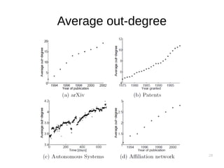
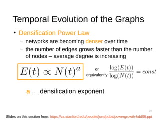
Temporal evolution of graphs
● Jure Leskovec, Jon Kleinberg, and Christos
Faloutsos: “Graphs over time: densification
laws, shrinking diameters and possible
explanations.” In KDD 2005. [DOI][Slides]
● Two main findings:
– Diameter tends to shrink
– Average degree tends to increase](https://image.slidesharecdn.com/6qfb9tczqegev93zz5tu-signature-174179124c8bf94a633d0f75ae58d0985739d29f77acf7ddb862c471a419c3cd-poli-151222094555/85/Graph-Evolution-Models-25-320.jpg)
![36
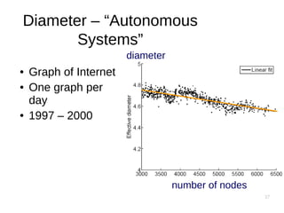
Diameter – ArXiv citation graph
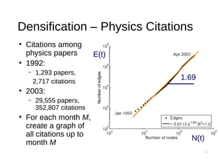
● Citations among
physics papers
● 1992 –2003
● One graph per
year
time [years]
diameter
https://cs.stanford.edu/people/jure/pubs/powergrowth-kdd05.pptSlides on this section from:](https://image.slidesharecdn.com/6qfb9tczqegev93zz5tu-signature-174179124c8bf94a633d0f75ae58d0985739d29f77acf7ddb862c471a419c3cd-poli-151222094555/85/Graph-Evolution-Models-34-320.jpg)
![38
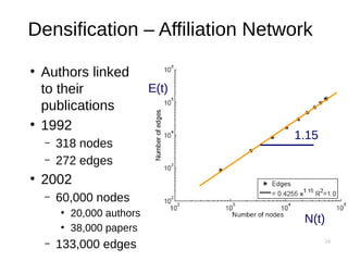
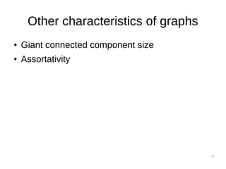
Diameter – “Affiliation Network”
●
Graph of
collaborations in
physics –
authors linked to
papers
●
10 years of data
time [years]
diameter](https://image.slidesharecdn.com/6qfb9tczqegev93zz5tu-signature-174179124c8bf94a633d0f75ae58d0985739d29f77acf7ddb862c471a419c3cd-poli-151222094555/85/Graph-Evolution-Models-36-320.jpg)
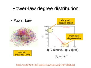
![39
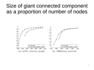
Diameter – “Patents”
●
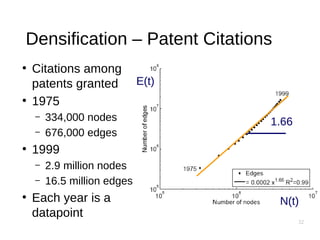
Patent citation
network
●
25 years of data
time [years]
diameter](https://image.slidesharecdn.com/6qfb9tczqegev93zz5tu-signature-174179124c8bf94a633d0f75ae58d0985739d29f77acf7ddb862c471a419c3cd-poli-151222094555/85/Graph-Evolution-Models-37-320.jpg)

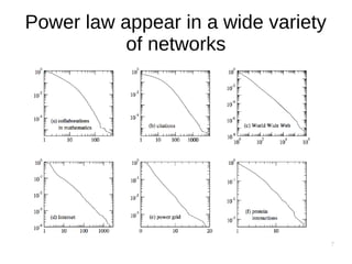
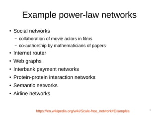
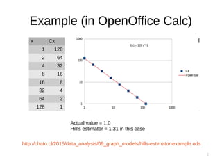
The document outlines algorithmic methods for modeling and mining large graphs, focusing on characteristics such as power-law degree distribution, densification, and graph evolution. It discusses various examples of networks exhibiting power-law behavior and introduces the concept of preferential attachment as a model of graph growth. Additionally, it explores metrics such as effective diameter and assortativity in understanding the structure and dynamics of networks over time.