The document provides instructions for running the DMAP software to analyze drought indices. It describes: 1. How to open an input Excel file, select the sheet, and assign variables such as date, temperature, and precipitation. 2. How to select drought indices like SPI on the "Drought Indices" tab, choose calculation frequency and time period, generate index values, export results to Excel, and plot the output. 3. How to calculate the severity and duration of drought events by setting index borders on the "Severity" panel and viewing the results table.

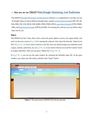
1. 1
 How can we run DMAP V.1.0 (Drought Monitoring And Prediction)?
The DMAP (Drought Monitoring And Prediction) software is a comprehensive tool that can run
18 drought indices in three different drought types, namely meteorological drought (SPI, PN, DI,
RAI, RDI, ZSI, CZI, MCZI, EDI, KBDI, PDSI, PHDI, SPEI), agricultural drought (ETDI, SMDI,
ARI), and hydrological drought (SWSI and SDI). For running this software you can follow these
steps one by one.
Step 1:
The DMAP tool has 4 tabs, that in this version the point option is active, the region ability will
active in the next version (Fig. 1). For starting the software, first select the first tab, “Input Excel
File” (Fig.2 No. 1). If you want to browse a text file, first you should assign your delimiter (such
a space, comma, semicolon, etc.) (Fig.2 No. 2), if you want to browse an excel file it doesn’t need
to assign a delimiter. Then you can press “Open File” (Fig.2 No. 3).
In Fig.2 No. 4, you can see the open window for selecting the desirable input file. In the open
window, you select your file easily, and then click “Open” button.
Figure 1. The main screen of DMAP tool with the main tabs.

2. 2
According to the Fig. 3 No. 1, you can see all the sheets that are available in your excel file, so
select the proper sheet. In this example we select “Mashhad” sheet that it has several important
weather data of Mashhad synoptic station. If your excel file sheet has header of columns so please
select the “first Row is header” option (Fig. 3 No. 2), also in “Input Timing” you can select time
scale of the input file. In the presented example here, the input data are in daily sale, so we check
“Daily” (Fig. 3 No. 3).
Figure 2. The input excel file tap and the details.
1
2 3
4
Figure 3. Browse your input file and select your sheet

3. 3
After the desirable sheet was selected then it is the turn of assignments of weather variables.
Therefore, as presented in Fig. 4 No.1, you can apply the format of your time scale. If your time
data have a format like the 1986, then you should select “YYYY” in the combo box (Fig. 4). In
this example for time, there are just the Julian years for each day of year.
Then you should assign the header of each column. Attention please, as you see in Fig. 5, in this
example the first column was assigned to the “Date”, but there is not any special order for the
columns, and this is actually one of the best advantage of the DMAP tool. Also, as presented in
Fig.6 assign all the variables, if one or more columns are not necessary to assign, you should
remain them with any header.
Figure 4. Select the format of time.
Figure 5. Assign the variables.

4. 4
As you see in Fig. 6, in this sample input file the second column not necessary for assignment, so
the header is “None“(Fig. 6 No. 1) and it doesn’t consider for calculation drought indices. In this
sample the first column is “Date”, and others are respectively equal to “None”, “Tmax”, “Rain”,
and “T”, that Tmax refers to maximum temperature, Rain for the amount of precipitation, and T
refers to mean of temperature. Finally, press the “Load Data” button (Fig. 6 No. 2). Then you will
face to a small window “Data loaded”, click it and go to the next step (Fig. 7).
Figure 6. Assign all the variables, without any specific order.
2
Figure 7. Click the “Data Loaded” button.

5. 5
Step 2:
In this step please click on the “Drought Indices” tab in the Tab menu. The first panel in this screen
is related to the “Calculator” setting. According to the Fig. 8, you can see a small panel that its
name is “Timing”. In this panel you can set the start (Fig. 8) and the end (Fig. 9) years.
Figure 9. Select the end year in the “Timing” panel.
Figure 8. Select the start year in the “Timing” panel.

6. 6
Then you can select your desirable index from the “Indices” panel, then the “Frequency” panel
will highlighted for selecting. According to the selected index in “Indices” panel, the “Frequency”
panel has different type. In this example, since the “SPI” index (Fig. 10 No. 1) was selected so the
“Frequency” panel has three types, namely Yearly, Seasonally, and Monthly. As you see in Fig.
10, we selected “Yearly” type for calculation of SPI output (Fig. 10 No. 2).
Figure 10. Select the end year in the “Timing” panel.
Figure 11. Generate value of the selected index.

7. 7
By clicking “OK” button, the index’s value was calculated if the user wants to see the values, by
clicking the “Send to table” button (Fig. 12 No. 1), the user can see the values of selected drought
index in the “Output Data” table (Fig. 12 No. 2). If the user wants to export the outputs of the
index, he/she can click on the “Export To Excel” button that it is located in the right corner of the
screen (Fig. 12 No. 3). By clicking this button, a browse window will open to select a name for
the excel output file in a wanted path (Fig. 13). When the file successfully saved, the user can see
a small dialog box that will show a message with this content “The file was saved successfully”
(Fig. 14).
Figure 12. Send the output of selected index to the table.
Figure 13. Select a name and path for the selected index’s outputs in an excel file.

8. 8
If you want to plot the values of calculated index, you can set some characteristics of the plot
settings. You can do this settings in the “Plots” panel as shown in Fig. 15 No.1. In the “Tool”
option, first the user can select desirable domain for start and end year. In “Chart Options”, you
can type a proper title (Fig. 15 No.2, in this sample we have typed “SPI Mashhad”) for your graph
and also if you want your graph has horizontal line in the background you can click the “H-Line”
option (Fig. 15 No.3).
Figure 14. Select a name and path for the selected index’s outputs in an excel file.
Figure 15. Assign some characteristics for Setting of the plot.
1

9. 9
You have two options for selecting the color of the graph, namely “Grayscale” and “Color plot”.
If you don’t select other colors you can just click “Grayscale” option, otherwise click on the combo
box, then you can see lots of different colors and as well you can select one of them for the graph
(Fig. 16). At last, you can choose your “type of plot” (Fig. 16 No. 1). There are three options,
namely “BoxPlot”, “Linear”, and “Columnar” (Fig. 16 No. 1). Finally, after selecting the type of
graph you can click on the “Plot” button, and observe the selected graph. The selected graph in
this example is “Linear”, so in Fig.17 you can see it, according to this graph since the typed titled
was “SPI Mashhad”, so in the presented graph you can see this title. If you want to change it you
can easily do it by typing another one in the “Chart Option” panel.
Figure 16. Select the proper color and title for the plot.
Figure 17. Plot the desirable graph for the output of index.

10. 10
In Fig. 18 and Fig. 19, we plotted the yearly boxplot of SPI values, and the yearly columnar plot
of SPI, respectively by clicking the “Boxplot” and “Columnar” options.
Figure 18. The yearly Boxplot for the output of SPI.
Figure 19. The columnar plot for the yearly output of SPI.

11. 11
Step 3:’Calculate Severity and Duration’
One of the most important characteristic that Agrimetsoft was considered in the DMAP
(Drought Monitoring and Prediction) software, is calculating severity and duration of
drought event. In Fig. 20 and in the right side of screen, you can see a panel with the
name of “Severity”. In this panel for calculating the severity and duration of drought
in a specific region, first of all you should determine the range of the desirable drought,
for example in SPI the specific border of drought classification is less than -0.99. This
border can easily find for every index according to the origin paper that was published
for each index. You can select one of the two options, namely “More than” or “Less
than”. Fig. 21 presented the severity and durations of drought index. In this sample, we
have calculated SPI, so the label of “Y” axe is “SPI”. Also, as you can see in Fig. 21at
the top the graph, there is a table that
Figure 20. The severity panel for assign border.

12. 12
Figure 21. The columnar plot for the yearly output of SPI.
Figure 21. The values of severity and duration.

13. 13
Figure 6

14. 14