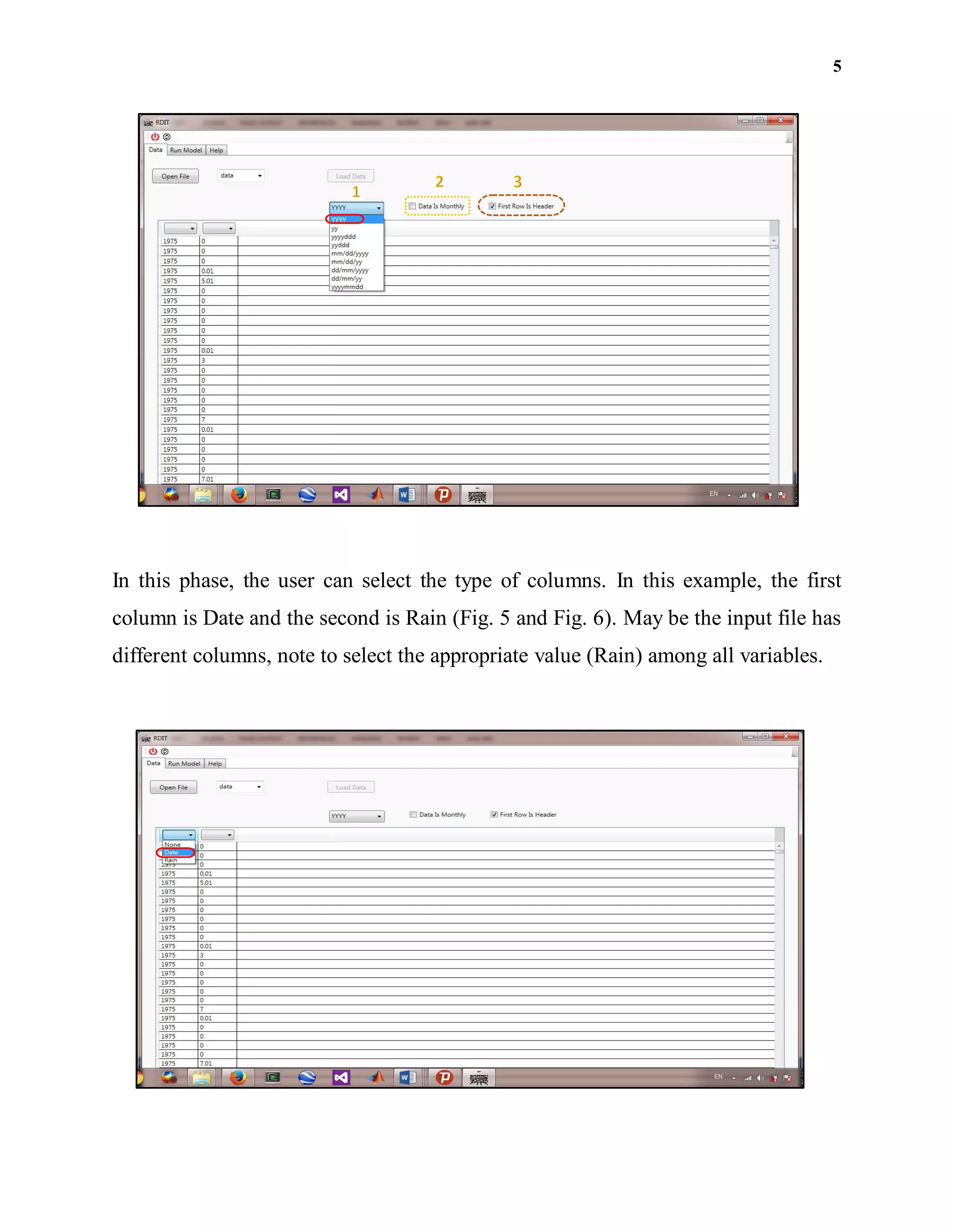
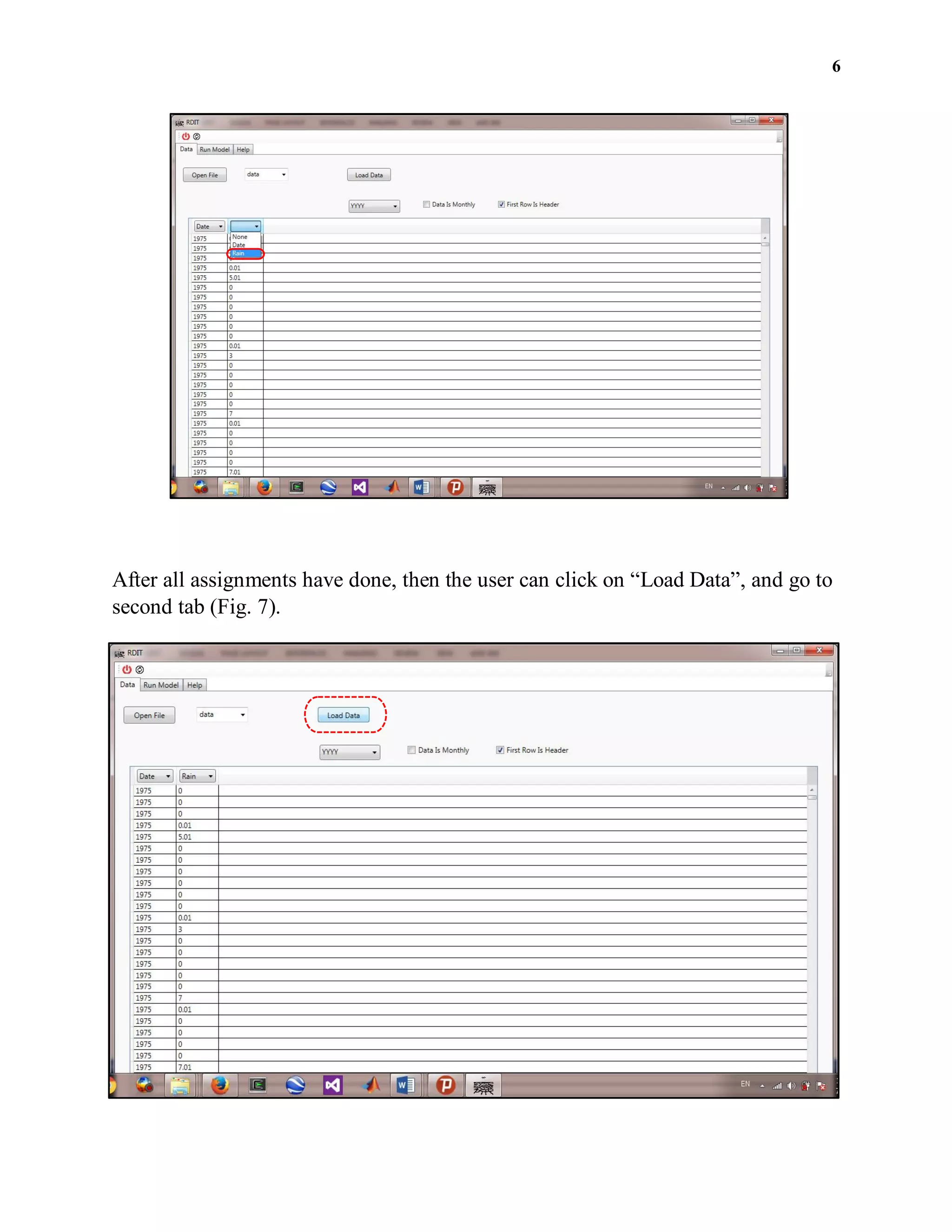
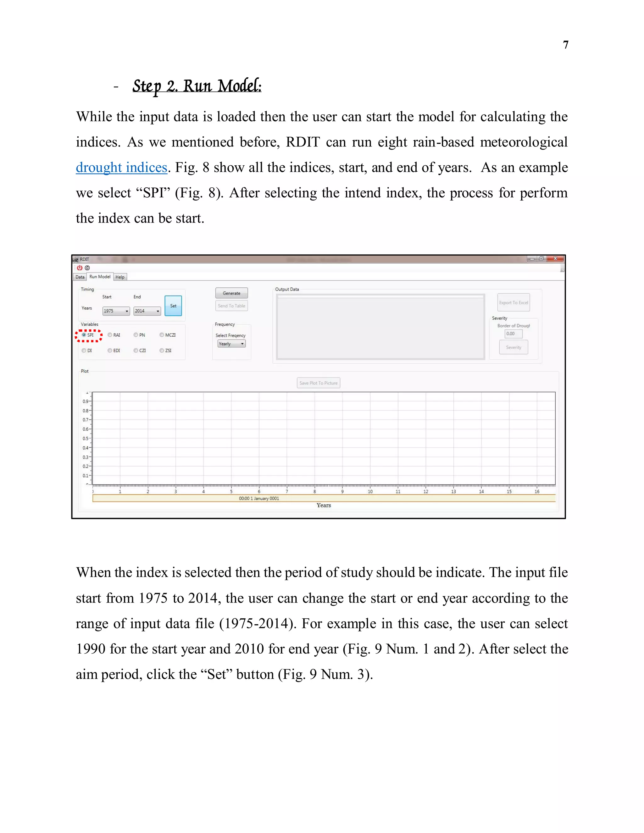
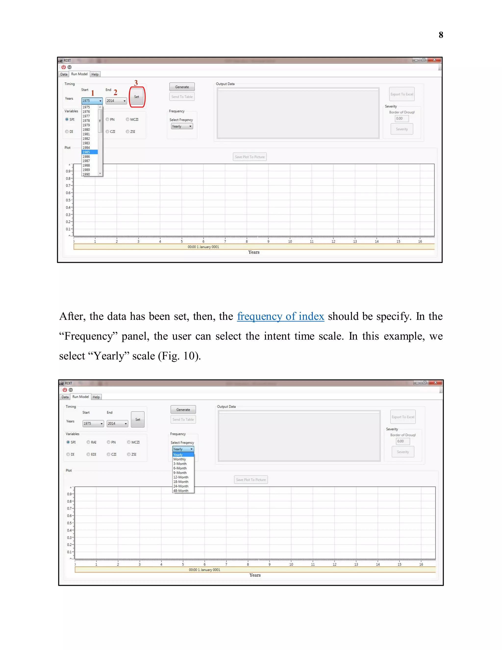
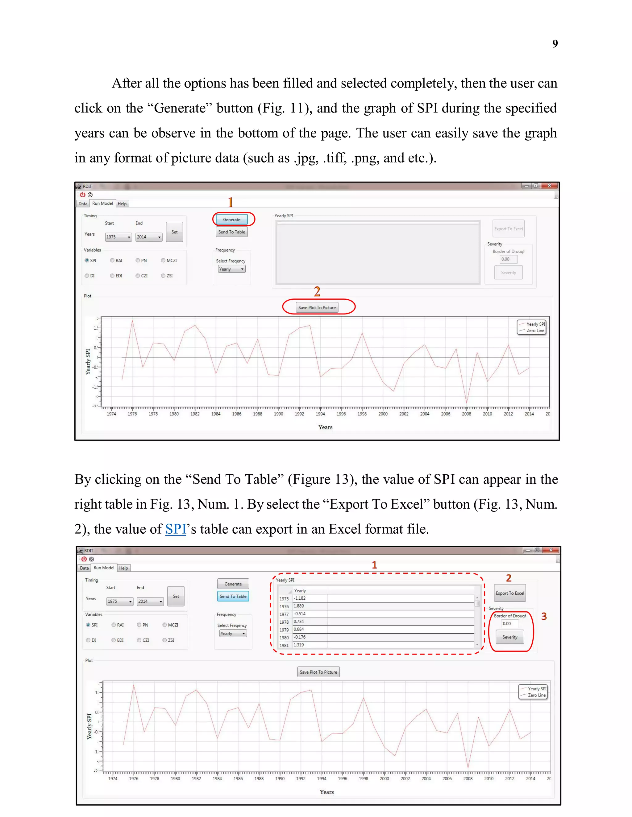
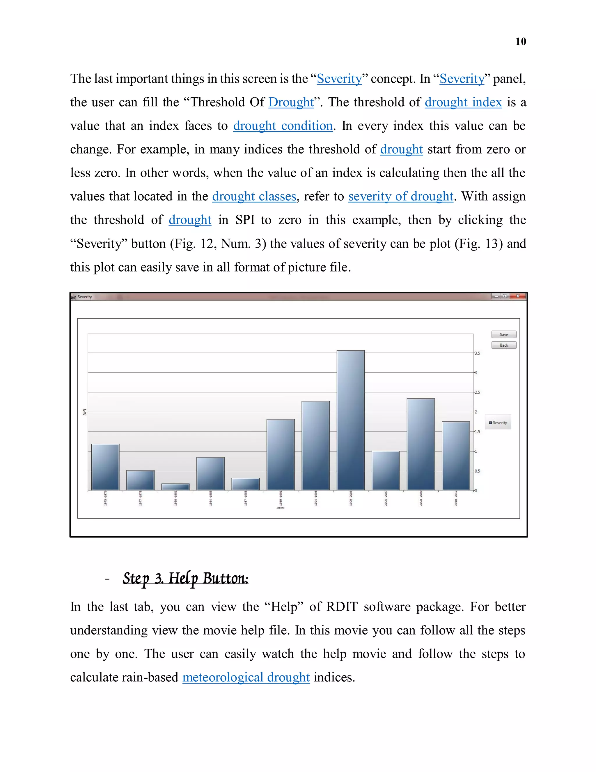
This document describes how to calculate meteorological drought indices using the RDIT software. It discusses 8 main indices: SPI, DI, PN, RAI, EDI, CZI, MCZI, and ZSI. The document then outlines the 3 step process to use RDIT: 1) open the data file and assign data properties, 2) run the model by selecting an index, time period, and frequency, and 3) view the output graph and export results. Severity thresholds can also be set to identify drought conditions. A help movie is available to guide users through each step of the process.

1. 1
 How can we calculate meteorological drought indices?
There are eight famous rain-based meteorological drought indices. We calculate
this indices as following:
- SPI (Standardized Precipitation Index)
SPI is a widely recognized tool for characterizing meteorological drought
(Hayes et al., 1999; Deo, 2011). McKee et al. (1993, 1995) defined SPI across
different timescales (1, 3, 6, 12, 24 and 48 months). The Standardized Precipitation
Index (SPI) is widely used for defining and monitoring meteorological droughts.
For the details of calculation, refer to McKee et al. (1993). The range of SPI is
between +2.0 and −2.0.
- DI (Deciles Index)
The deciles index (DI) was defined by Gibbs and Maher (1967). For calculating
this index, we should to sort the precipitation data in a specific format. In this
approach proposed by Gibbs and Maher the total monthly precipitations from a
long record is first ranked from highest to lowest to construct a cumulative
frequency distribution. The severity of drought can be assessed by comparing the
quantity of rainfall in a particular month or several months duration with the long
time cumulative distribution of rainfall values for that time.
- PN (Percent of Normal Index)
The PN index for a specific location was described by Willeke et al. (1994) as
percent of normal precipitation. The PNI index is simple, by definition, easy
to calculate, and is easy understood by a general audience (Smakhtin and
Hughes 2004). The index can be calculated for a variety of time scales.
- RAI (Rainfall Anomaly Index)

2. 2
The RAI was developed by van Rooy (1965), and incorporates a ranking
procedure to assign magnitudes to positive and negative anomalies, namely it
considers two phases, positive precipitation anomalies and negative precipitation
anomalies. Refer to van Rooy (1965) for details of calculations.
- EDI (Effective Drought Index),
Byun and Wilhite (1999) developed the EDI. It is the only index that was specifically
designed to calculate daily drought severity. For detailed explanations, please refer
to Byun and Wilhite (1999). The "drought range" of the EDI indicates extreme
drought at EDI ≤ -2, severe drought at -2.0 < EDI ≤ -1.5, and moderate drought at -
1.5 < EDI ≤ -1.0. Near normal conditions are indicated by -1.0 < EDI ≤ 1.0.
- CZI (China-Z Index), and MCZI (Modified CZI),
The CZI is based on the Wilson–Hilferty cube-root transformation. In the
calculating of CZI, we assuming that precipitation data follow the Pearson Type III
distribution. To calculate the MCZI, the median of precipitation is used instead of
the mean of precipitation in the calculation of the CZI.
- ZSI (Z-Score Index)
The ZSI is more analogous to CZI, but without the requirement for fitting
precipitation data to either Gamma or Pearson Type III distributions. The more the
value of this index, the more severe the drought. For calculating of ZSI, we use mean
monthly precipitation and standard deviation of precipitation in a specific month.
 How can we use RDIT software?
For calculating rain-based meteorological drought indices we need a useful
software application that it can apply for calculating this indices. To use the RDIT
application the user can follow this steps.

3. 3
- Step 1. Open Data File:
At the main screen of RDIT, you can see three tabs (Fig. 1). First tab is “Data”. In
this tab user can browse the input file of data. By clicking on the “Open file”, the
user can select input file (Fig. 2) with Excel format file.

4. 4
The input file can be in different time scale, namely daily, and monthly. When the
user browse the input file, the sheets of the file is appear in the first menu (Fig. 3).
According to Fig. 3, the selected file has two sheets: data and sheet1. The user can
select every sheet that he/she wants.
By selecting the intent sheet, you can observe the data of input file. Now, in this step,
some assignment should be apply. According to Fig. 4, the format of data should be
select. In this example the format of “YYYY” has been selected (Num. 1, in Fig. 4).
Then, if the input data is in monthly format, please select the checkbox of “Data is
Monthly” (Num. 2, in Fig. 4). Then, if the first row of input file has header, sign the
checkbox of “First Row Is Header” (Num. 3, in Fig. 4).

5. 5
In this phase, the user can select the type of columns. In this example, the first
column is Date and the second is Rain (Fig. 5 and Fig. 6). May be the input file has
different columns, note to select the appropriate value (Rain) among all variables.

6. 6
After all assignments have done, then the user can click on “Load Data”, and go to
second tab (Fig. 7).

7. 7
- Step 2. Run Model:
While the input data is loaded then the user can start the model for calculating the
indices. As we mentioned before, RDIT can run eight rain-based meteorological
drought indices. Fig. 8 show all the indices, start, and end of years. As an example
we select “SPI” (Fig. 8). After selecting the intend index, the process for perform
the index can be start.
When the index is selected then the period of study should be indicate. The input file
start from 1975 to 2014, the user can change the start or end year according to the
range of input data file (1975-2014). For example in this case, the user can select
1990 for the start year and 2010 for end year (Fig. 9 Num. 1 and 2). After select the
aim period, click the “Set” button (Fig. 9 Num. 3).

8. 8
After, the data has been set, then, the frequency of index should be specify. In the
“Frequency” panel, the user can select the intent time scale. In this example, we
select “Yearly” scale (Fig. 10).

9. 9
After all the options has been filled and selected completely, then the user can
click on the “Generate” button (Fig. 11), and the graph of SPI during the specified
years can be observe in the bottom of the page. The user can easily save the graph
in any format of picture data (such as .jpg, .tiff, .png, and etc.).
By clicking on the “Send To Table” (Figure 13), the value of SPI can appear in the
right table in Fig. 13, Num. 1. By select the “Export To Excel” button (Fig. 13, Num.
2), the value of SPI’s table can export in an Excel format file.

10. 10
The last important things in this screen is the “Severity” concept. In “Severity” panel,
the user can fill the “Threshold Of Drought”. The threshold of drought index is a
value that an index faces to drought condition. In every index this value can be
change. For example, in many indices the threshold of drought start from zero or
less zero. In other words, when the value of an index is calculating then the all the
values that located in the drought classes, refer to severity of drought. With assign
the threshold of drought in SPI to zero in this example, then by clicking the
“Severity” button (Fig. 12, Num. 3) the values of severity can be plot (Fig. 13) and
this plot can easily save in all format of picture file.
- Step 3. Help Button:
In the last tab, you can view the “Help” of RDIT software package. For better
understanding view the movie help file. In this movie you can follow all the steps
one by one. The user can easily watch the help movie and follow the steps to
calculate rain-based meteorological drought indices.