Using Microsoft Excel4 Charts

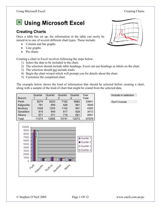
1. Using Microsoft Excel Creating Charts
Using Microsoft Excel
Creating Charts
Once a table has set up, the information in the table can easily be
turned in to one of several different chart types. These include:
• Column and bar graphs
• Line graphs
• Pie charts
Creating a chart in Excel involves following the steps below:
1) Select the data to be included in the chart.
2) The selection should include table headings. Excel can use headings as labels on the chart.
3) The selection should not include totals.
4) Begin the chart wizard which will prompt you for details about the chart.
5) Customise the completed chart.
The example below shows the kind of information that should be selected before creating a chart,
along with a sample of the kind of chart that might be crated from the selected data.
Quarter Quarter Quarter Quarter Year Include in selection
Branch 1 2 3 4 Total
Perth 8274 9203 7182 8982 33641 Don't include
Kalgoorlie 781 859 928 981 3549
Bunbury 1029 1203 1102 991 4325
Geraldton 819 849 817 928 3413
Albany 671 571 718 691 2651
Total 11574 12685 10747 12573 47579
© Stephen O’Neil 2005 Page 1 Of 12 www.oneil.com.au/pc

2. Using Microsoft Excel Creating Charts
Exercise 1. Creating a Column Graph
1) Open the Grades.xls file that you have been working on previously. We will create a graph to
show the results for the students each term.
2) Select the cells A5:E14. Note that this includes headings but no totals.
3) Click the Chart Wizard icon.
The chart wizard will begin. As you can see from the title bar of the wizard, this will be the first of
four steps. The first step is to choose a chart type.
4) From the list of Chart Types, make sure Column is selected.
5) In the list of Chart sub-types, choose the first option in the second row as shown above.
6) Click and hold the Press and Hold to View Sample button to see a basic preview of your chart.
7) Click Next to proceed to the second step of the wizard.
© Stephen O’Neil 2005 Page 2 Of 12 www.oneil.com.au/pc

3. Using Microsoft Excel Creating Charts
8) The second step allows you to confirm that the correct data is selected for the chart. It has
automatically selected to use the student names along the bottom of the chart. For Series In,
select Rows to have the terms along the bottom of the chart.
9) Click the Series tab at the top to see what labels and series are being used for the chart.
Notice that for each student name in the Series list, you are shown which cell the Name of the series
comes from and which cell range the Values for that series come from. You can use this to add
additional students if needed. The Category (X) axis labels box specifies which cells the labels along
the bottom of the chart will come from (Term 1-4).
© Stephen O’Neil 2005 Page 3 Of 12 www.oneil.com.au/pc

4. Using Microsoft Excel Creating Charts
10) Click Next to continue to the third step of the wizard.
This step allows you to add additional information such as a chart title. These options can all be
changes later but we will use some of them now.
11) In Chart Title enter Eastern Goldfields Student Results.
12) Click Next to proceed to the last step of the wizard.
This step allows you to place the chart on the current sheet, or to place it on an entirely new sheet
(more on working with sheets later).
13) Make sure the second option is selected as shown above and click Finish.
A chart will now be created on the sheet. Since the chart’s probably been placed overlapping your
table, you’ll probably want to move it.
© Stephen O’Neil 2005 Page 4 Of 12 www.oneil.com.au/pc

5. Using Microsoft Excel Creating Charts
14) Position your mouse pointer
over a blank area of the chart
and drag the chart until the
outline of the chart is below
your table as shown to the
right.
Exercise 2. Modifying a Chart’s Format
When a chart has been created, you can customise almost anything about the way the chart looks.
When a chart is selected, the chart toolbar will appear.
This toolbar contains icons that can be used to modify the chart in several ways. Most parts of a chart
can be selected and formatted individually as well.
1) Click on the title of the chart.
2) Use the Font Formatting box in the toolbar to change the font style to Comic Sans MS.
© Stephen O’Neil 2005 Page 5 Of 12 www.oneil.com.au/pc

6. Using Microsoft Excel Creating Charts
3) Click on one of the dark blue bars in the chart (these should be the ones for Lita Alexander).
All of the bars for that student (series) will be selected.
4) Right-click one of the selected bars and select Format Data Series, or click the icon on the
chart toolbar.
5) Click a colour from the colour palette shown.
6) Click OK. All the bars for that student will change to the new colour.
7) Click one of the selected bars. That bar alone will be selected. Clicking a bar from a selected
series a second time means that you will be able to change the formatting from that one
separately from the others in the series.
© Stephen O’Neil 2005 Page 6 Of 12 www.oneil.com.au/pc

7. Using Microsoft Excel Creating Charts
Many parts of the chart can be formatted by double clicking on them as well.
8) Double click on the background of the chart to access the Format Walls options.
9) Click the Fill Effects Button
10) Click Two Colours and then choose two colour for the gradient background as shown below.
11) Click OK to confirm your choices and click OK again to exit the Format Walls options. The
background area of your chart will now be formatted using the two colours you selected.
12) Try formatting other areas of the chart by double-clicking on them and then changing the
options that appear.
© Stephen O’Neil 2005 Page 7 Of 12 www.oneil.com.au/pc

8. Using Microsoft Excel Creating Charts
Exercise 3. Changing Chart Type
1) Make sure your chart is still selected (it should still have the black selection squares around it
if it is).
2) Click the arrow next to the Chart Type icon on the Chart toolbar. A list of
chart types like the one to the right will appear.
3) Click on the 3D Column Chart icon (the one with the circle around it to the right.
Your chart will now change to a 3D Column format.
4) Use the Sizing handles to make the chart bigger. When you make the
chart bigger the text on the labels may also become bigger.
5) Double-click the labels on the X axis to show the formatting options.
6) When the Format Axis options appear, change the font size to 10 and the alignment angle to 60º
so that the axis labels look like the example below.
7) Format the side axis labels in a similar way so that they look like the example below.
8) Now that there are labels along each axis, there is no longer any need for the chart legend.
Click on the legend and then press the [Delete] key to remove it. This will leave more room
for the chart itself.
© Stephen O’Neil 2005 Page 8 Of 12 www.oneil.com.au/pc

9. Using Microsoft Excel Creating Charts
Exercise 4. Rotating a Chart
1) Click on the chart walls (the coloured area behind the chart). Small black squares will appear
around the corners of the 3D chart area.
2) Move your mouse over one of the squares until a corners caption appears as shown below.
3) Click and hold your mouse and then drop to rotate the chart. A wire frame view will appear
to help you position the chart on the angle you want.
4) When the chart is on an angle that suits you, release the mouse button to complete the
change.
© Stephen O’Neil 2005 Page 9 Of 12 www.oneil.com.au/pc

10. Using Microsoft Excel Creating Charts
Exercise 5. Creating a Pie Chart
One of the differences between a pie chart and a normal chart is that a pie chart will only show data
for one series at a time. In the following exercise, we’ll create a pie chart from the year’s data.
We need to begin by selecting the names of the students (to be used as labels) and the data itself.
1) Select the cells with the student names including the student heading (A5:A14). Since we need
to select more than one group of cells we’ll need to use the [Ctrl] key.
2) Hold down [Ctrl] and select the cells with the year data (F5:F14)
A5:A14 and F5:F14 should now be selected.
3) Click the chart wizard icon to begin creating the chart from the selected data.
4) Select Pie for the Chart type and the second sub-type as shown in the example above.
5) Click Next to continue
6) Confirm that the selected cell range reads =Sheet1!$A$5:$A$14,Sheet1!$F$5:$F$14 and click
Next to continue.
© Stephen O’Neil 2005 Page 10 Of 12 www.oneil.com.au/pc

11. Using Microsoft Excel Creating Charts
7) Change the Chart title to Student Marks for the Year and click Next to continue.
8) For the final step, select As new sheet and enter Pie Chart for the name of the sheet.
9) Click Finish to complete the chart.
© Stephen O’Neil 2005 Page 11 Of 12 www.oneil.com.au/pc

12. Using Microsoft Excel Creating Charts
10) Click on the chart to select it.
11) Right-click on the selected chart and select Format Data Series.
12) Select the Data Labels tab and select the Category Name option as
shown below.
13) Clock OK to make the change. The name of each student will now appear
next to their pie slices. This means we no longer need the chart legend so we
can delete it to make more room.
14) Click the legend to select it and press [Delete].
15) Click the chart to select it again and then click the pie piece for Lita
Alexander. That piece will now be the only one selected.
16) Slowly drag that piece away from the centre of the pie. This technique is
often used to emphasise a certain figure (such as the highest mark).
You can return to the original sheet (Sheet 1) at any time by using the sheet tabs at the bottom of the
window.
© Stephen O’Neil 2005 Page 12 Of 12 www.oneil.com.au/pc