The document provides instructions for using NetCDF Extractor V2.0 to extract data from NetCDF files in 3 steps: 1. Users can either load a single file (Option 1) or multiple files (Option 2) from the main menu. For multiple files, the program will merge the data. 2. In the extraction panel, users select the variable, dimensions, and tools to define the region of data to extract. 3. The extracted data is displayed and can be exported to Excel. Calculations like averaging can also be performed on the extracted data region.

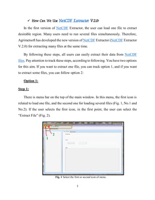
1. 1
 How Can We Use NetCDF Extractor V.2.0?
In the first version of NetCDF Extractor, the user can load one file to extract
desirable region. Many users need to run several files simultaneously. Therefore,
Agrimetsoft has developed the new version of NetCDF Extractor (NetCDF Extractor
V.2.0) for extracting many files at the same time.
By following these steps, all users can easily extract their data from NetCDF
files. Pay attention to track these steps, according to following. You have two options
for this aim. If you want to extract one file, you can track option 1, and if you want
to extract some files, you can follow option 2:
Option 1:
Step 1:
There is menu bar on the top of the main window. In this menu, the first icon is
related to load one file, and the second one for loading several files (Fig. 1, No.1 and
No.2). If the user selects the first icon, in the first point, the user can select the
“Extract File” (Fig. 2).
Fig. 1 Select the first or second icon of menu.
1
2

2. 2
Then, browse the .nc file from your system (Fig. 3). When the input file was
selected, the user can observe all the variables of the file at the left corner of the
screen (Fig. 4). According to the loaded file in this example, the main variable of
this file is “tas” (temperature), so you can selected the related radio button as Fig. 4,
No. 1. In this screen you can see two tabs: 1- View All Data, and 2- Extract Data.
At this section, the user start the process by the first tab (View All Data). In this
tab, the user can just view the content of the file, and he/she can’t extract the data at
this tab. The example browsed file (in this help file) is the mean temperature of
“MIROC4h_rcp45…” from CMIP5 data. You can see different variables such as tas,
lon, lat, time, and height. By selecting one of the variables you can see the
descriptions of them. In the Fig. 4, No. 1, the “tas” was selected, so the “dimension”
panel shows three variables related to “tas” (Fig. 4, No. 2). Pay attention, in this part
with three variables, when the user select time, so in the “Tool” panel (Fig. 3, No.
Fig. 2 Select the “Extract File” tab.

3. 3
3), you can see the value of “tas” for the selected time. It means that “time” is
variable (the user can choose every day from the first day of the file up to the end of
date of it), but “lon” and “lat” are constant. The user can easily save and export the
data to an Excel file. If you want to see the details of selected variable you can
expand the triangle sign that located in the “Variables” panel, for see them (Fig. 5).
At this information you can check the values of “lat”, “lon”,”unit”, and etc.
Fig. 3 Browse the desired file.
Fig. 4 Select the “Extract File” tab and the variable.
1
2
3

4. 4
Step 2:
Another tab that is located in the option 1, is “Extract Data” (Fig. 6, No. 1). In
this tab, you can see the name of selected variable with three panels: 1- Dimension,
2- Tools, and 3-Data. In the “Dimension” section, there is a useful tool with name
of “Grid Number Calculator” (Fig. 6, No. 2) that if the user doesn’t know the grid
number, he/she can use this button. If the user know the grid number, the calculator
tool was not used. In Fig. 6, No. 3, the user can enter the domains of his/her variables.
In this example the entered domains are: “time” from 32 with 28 number, “lat” form
122 with 3 number, and “lon” from 410 with 2 number. Pay attention, this domains
are related to the selected file. When the user wants to use the “Grid Number
Calculator”, the user can press the “Grid Number Calculator” button. As you see in
the Fig. 7, The user can enter the start and the end of domain with number of grid,
then the grid number will be appear in the blue space (Fig. 7).
Fig. 5 Expand the selected variable for further information.

5. 5
Fig. 6 The “Extract Data” tab with other options.
2
3
1
Fig. 7 The “Grid Number Calculator” with other options.

6. 6
In the second panel (“Tools”), the user can start the extract process by easy
setting. As you know, in this example there are three variables, namely, time, lat,
and lon. When the user wants to extract the data, he/she would select one of the
variable as a non-constant one. For better understanding, see the Fig. 8, No. 1. In this
example imagine that the user wants to extract the data of February 2006. So, in the
“Dimension” panel, he/she has entered 32 up to the end of February (Number=28).
Finally, in the “Tools” panel, the time option has been selected and in the combo
box (Fig. 8, No. 2).
In Fig. 9, at the third panel (“Data”), according to the example (February 2006),
through the “lat=122” with number of 3, and “lon=410” with number of 2, you can
view a table with three rows (3 numbers of lat) and two columns (2 numbers of lon).
1
2
Fig. 8 The “Tools” panel with other options.

7. 7
In this section the user can extract the selected data, furthermore he/she can
calculate data’s sum or average of the selected region. By clicking on the “Average”
button, the average values of selected area are presented in the “Data” table (Fig. 10,
No.1). By clicking on the “Export to Excel” the user can easily export the data to an
excel file (Fig. 10, No. 2).
Fig. 9 The “Data” panel with the first day of Feb. of 2006.
The values of lat
Fig. 10 The “Data” panel with Average of data
2
1

8. 8
Option 2:
Step 1:
The best advantage of NetCDF Extractor V.2.0 is open many files and extract
them, simultaneously for saving time of users. If the user needs to load several files
and extracts them as well, he/she can browse and select every file that he/she wants
(Fig. 11). From the main menu, the user can click on the load multi files option (Fig.
11, No.1). As you see in the Fig. 11, No.2, the user can select many files from the
files. In this example three files of MIROC4h was selected (Fig. 11, No.2). In the
“Extract Multi-Files” tab (Fig. 12, No.1), the panel (dash yellow-line) shows all the
data of files (Fig. 12, No. 2). In the “Unlimited Dimension”, the user can view all
different parts of an unlimited dimension of a variable (Fig. 12, No.3)
Fig. 11 load multi files
1
2

9. 9
In the “Options of Files” panel, you can see an important tip for merge NetCDF
files, namely: “Merge all files”: Start from 1 To 1096” (Fig. 13, No.1). Due to the
selected files in this example are related to the “temperature” of MIROC4h from
2006 up to 2008 (1096 days) so, all these files merge in this panel.
Fig. 12 See the panel of files
Fig. 13 The “Merge all files” sentence in the “Option of Files”.
1
1
2 3
1

10. 10
Step 2:
In the “Extract” panel, the user would write the exact name of variable that
present in the file (in this sample: “tas”, Fig. 14, No. 1). In the “Dimensions” section,
the user can enter the desirable area such as “option 1, Fig. 6, No.3”, by selecting
the area, the user can start the “extract” process (Fig. 14, No. 2). In this example, the
user write the start time from “366” up to “731”, it means that the 2007 was selected.
In the “Tool” panel, the user select “366” from the combo box (Fig. 14, No. 3).
According to the number of “lat=3” and the number of “lon=2”, hence, in the “Data”
panel you can view a table with two columns (lon) and three rows (lat), for the values
of “tas” in the day of 366 (Fig. 14, No. 4).
Fig. 14 The “Extract” panel with variable’s name.
1
2
3
4

11. 11
In the Fig. 15, No.1 you can see two options: “Sum” and “Average”, such as
option 1 in the Fig. 10, No.2. It is an important option for the user to calculate the
sum or average of a variable for the selected region Fig. 15, No.1. In this sample,
the “Average” button was selected and the average of values was presented in the
Fig. 15, No.2.
Finally, by clicking the “Extract” button the user can easily extract the value of
“tas” of the selected region. Through the “Export To Excel” button, the user can
export all the extracted data output in a excel file and it is so useful.
Fig. 15 The “Data” panel with Average of data
1
12