Downloaded 185 times

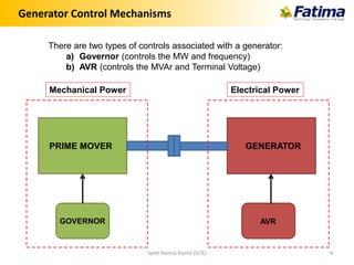
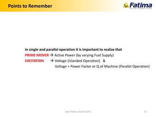

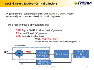
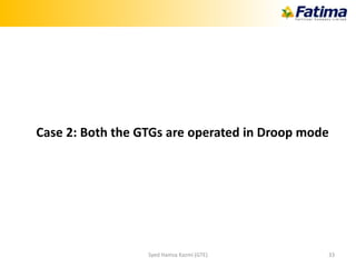
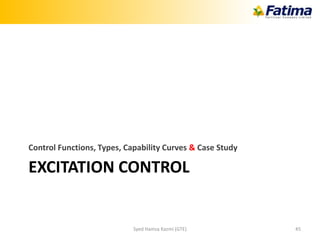
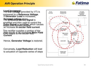
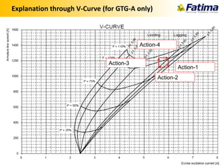
![Droop Mode – Explanation (Contd…)
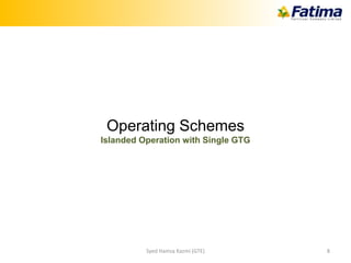
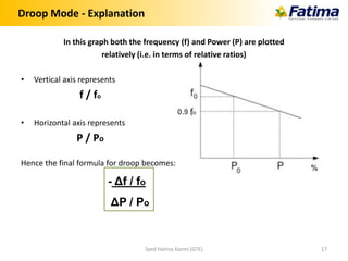
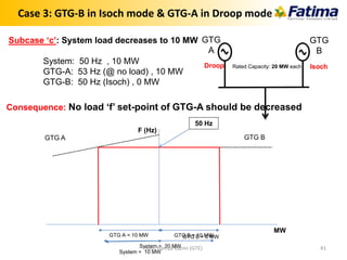
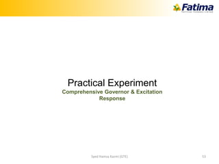
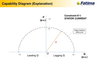
• Droop of 4 % :
– A change in 25% of the rated load of the machine results in a change of 1% in
its rated speed (Frequency)
– A change in 100% of the rated load of the machine results in a change of 4%
in its rated speed (Frequency)
– A 4 % change in frequency, means
• 50 Hz x 0.04 = 2 Hz or for a 4 pole generator, 1500 rpm x 0.04 = 60 rpm.
50 Hz
f [%]
60 rpm, 2Hz or
4%
P [%]
100%
Syed Hamza Kazmi (GTE) 18](https://image.slidesharecdn.com/16a2886c-168f-4c7b-af7b-cf6b748665d8-150513153825-lva1-app6891/85/Hamza-Kazmi-GTE-18-320.jpg)
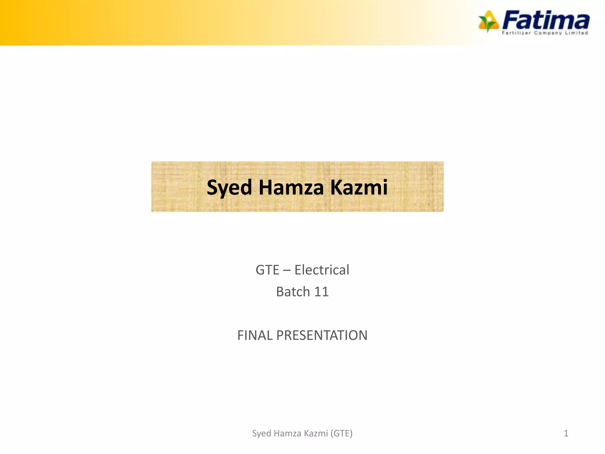
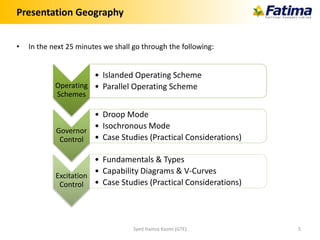
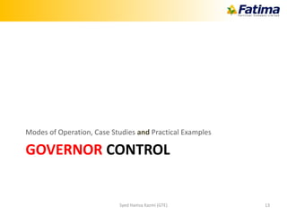
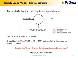
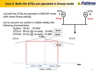
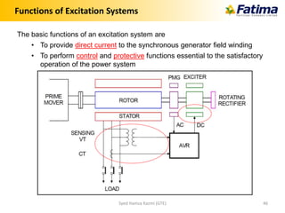
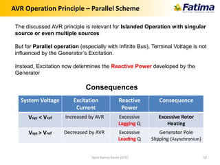
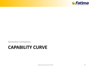
![Droop Mode – Explanation (Contd…)
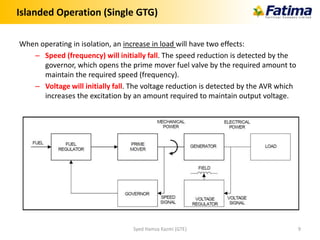
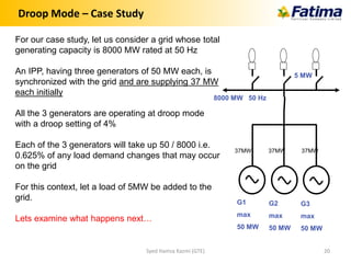
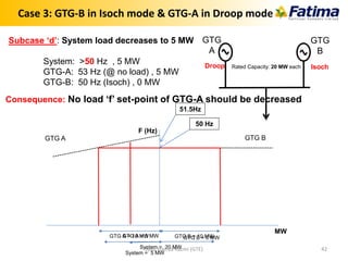
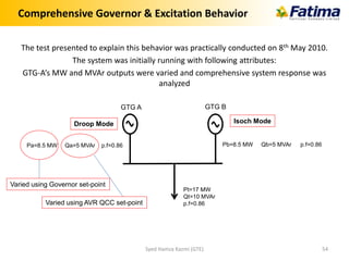
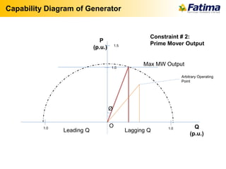
• Droop of 5 % :
– A change in 20% of the rated load of the machine results in a change of 1% in
its rated speed (Frequency)
– A change in 100% of the rated load of the machine results in a change of 5%
in its rated speed (Frequency)
– A 5 % change in frequency, means
• 50 Hz x 0.05 = 2.5 Hz or for a 4 pole generator, 1500 rpm x 0.05 = 75 rpm.
50 Hz
f [%]
75 rpm, 2.5Hz
or 5%
P [%]
100%
Syed Hamza Kazmi (GTE) 19](https://image.slidesharecdn.com/16a2886c-168f-4c7b-af7b-cf6b748665d8-150513153825-lva1-app6891/85/Hamza-Kazmi-GTE-19-320.jpg)
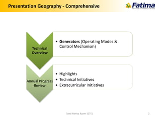
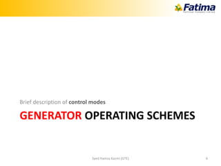
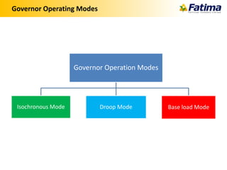
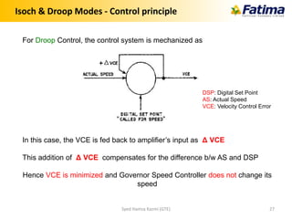
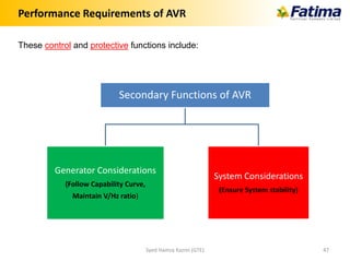
![4%
4%
f [%]
P [%]
100%
RAISE LOWERRAISE
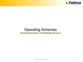
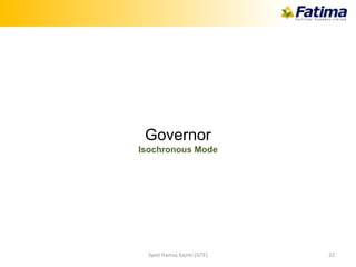
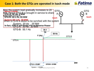
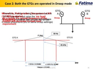
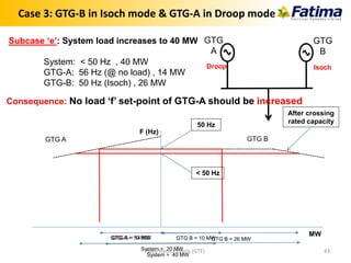
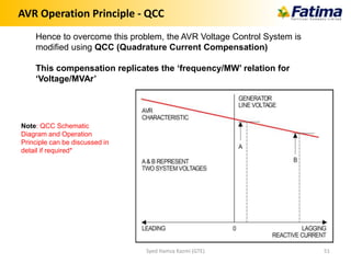
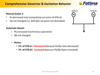
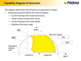
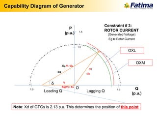
Droop Mode – Case Study
G1
max
50 MW
8000 MW 50 Hz
50 Hz
For any demand load, each generator must increase
50 MW / 8000 MW = 0.625% = 0.00625 of that demand
For 5 MW increase in demand
G1 = 0.00625 x 5 MW = 0.03125 MW 37.03125 MW
G2 = 0.00625 x (5- 0.03125) MW = 0.03105 MW 37.03105 MW
G3 = 0.00625 x (5- 0.03125- 0.03105) MW = 0.03086 MW 37.03086 MW
G2
max
50 MW
G3
max
50 MW
37 MW 37 MW 37 MW
What happens to frequency ?
50 Hz - (0.04 x 50 Hz x 5 MW / 8000 MW) = 49.9987 Hz
How?
Lets revisit the formula we just studied
5 MW
OPERATOR
Syed Hamza Kazmi (GTE) 21](https://image.slidesharecdn.com/16a2886c-168f-4c7b-af7b-cf6b748665d8-150513153825-lva1-app6891/85/Hamza-Kazmi-GTE-21-320.jpg)
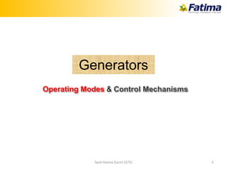
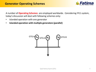
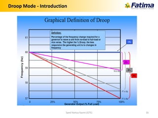
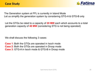
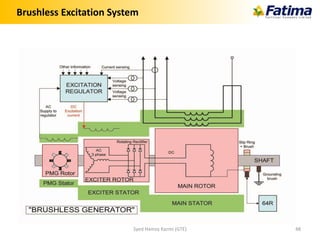
![f [Hz]
P [%]
100%50%
RAISE LOWER
SP Regulator
RAISE
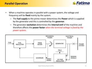
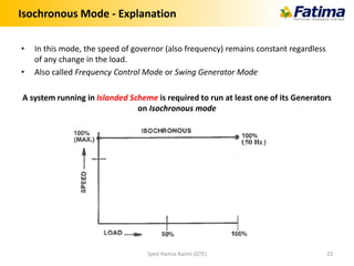
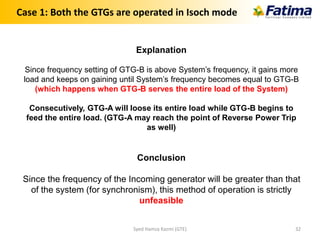
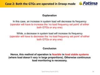
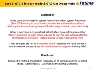
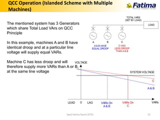
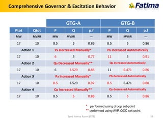
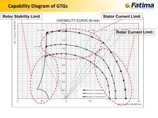
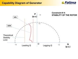
Isochronous Mode – Case Study
Referring to previous case, with one
of the three generators being
operated in Isoch mode
Syed Hamza Kazmi (GTE) 24](https://image.slidesharecdn.com/16a2886c-168f-4c7b-af7b-cf6b748665d8-150513153825-lva1-app6891/85/Hamza-Kazmi-GTE-24-320.jpg)


This document appears to be a presentation given by Syed Hamza Kazmi on generators. It includes: 1) An overview of generator operating modes and control mechanisms, including governor control which regulates frequency and active power, and AVR control which regulates voltage and reactive power. 2) A discussion of three generator operating schemes - islanded operation with a single generator, islanded operation with multiple generators in parallel, and parallel operation connected to a power system. 3) Examples of governor operating modes including droop mode and isochronous mode, including diagrams explaining how these modes work. 4) Three case studies examining different scenarios of generator control modes when operating in an islanded system