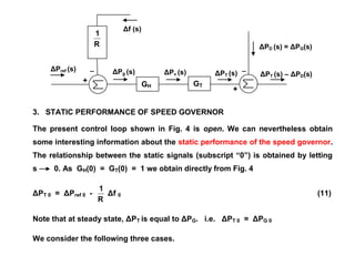
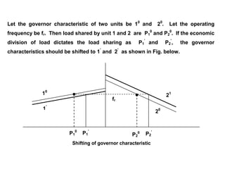
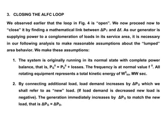
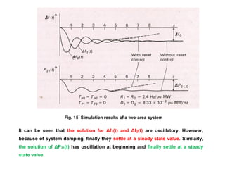
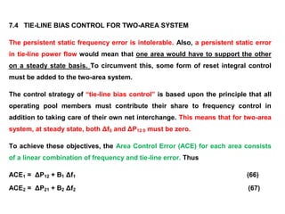
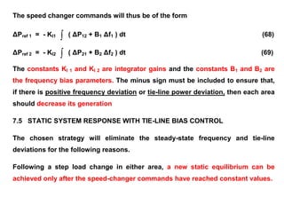
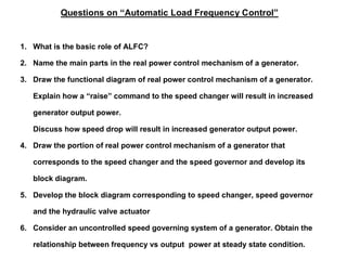
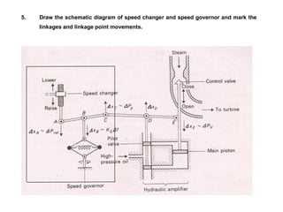
The document discusses automatic load frequency control (ALFC) which aims to maintain system frequency by balancing generator output power with changing load. It describes the key components in a single generator's real power control mechanism including the speed governor, hydraulic actuator, turbine, and generator. The speed governor senses changes in frequency and power setting to adjust the generator's real power output. The document presents models of these components and develops the primary ALFC control loop. It analyzes the static performance of the speed governor under different operating conditions and frequency-power characteristics.

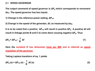
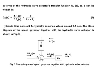

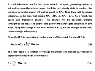
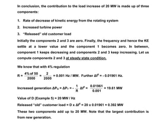
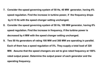
![Thus ΔPT – ΔPD =
dt
d
(Wkin) + D Δf (16)
Noting that f = f 0
+ Δf
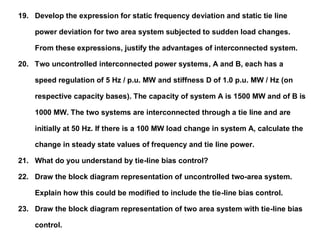
Wkin = W0
kin ( 0
0
f
f
f
) 2
= W0
kin [ 1 + 0
f
f
2
+ ( 0
f
f
)2
] W0
kin ( 1 + 2 0
f
f
) (17)
dt
d
(Wkin) = 0
kin
0
f
W
2
dt
d
( Δf )
Substituting the above in eq. (16)
ΔPT – ΔPD = 0
kin
0
f
W
2
dt
d
( Δf ) + D Δf MW (18)
By dividing this equation by the generator rating Pr and by introducing per-
unit inertia constant
H =
r
kin
0
P
W
MW sec / MW (or sec) (19)
it takes on the form
ΔPT – ΔPD = 0
f
H
2
dt
d
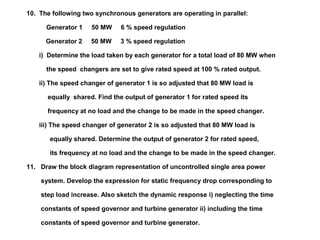
( Δf ) + D Δf pu MW (20)](https://image.slidesharecdn.com/alfc-230523014933-24458dcc/85/ALFC-pdf-27-320.jpg)
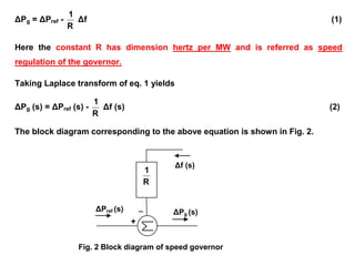
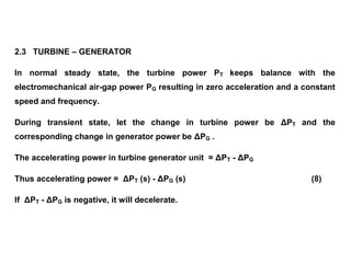
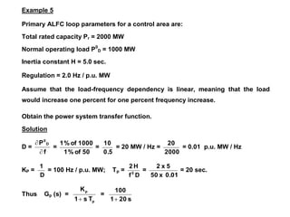
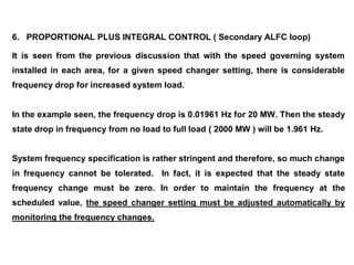
![ΔPT – ΔPD = 0
f
H
2
dt
d
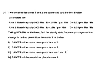
( Δf ) + D Δf pu MW (20)
The ΔP’
s are now measured in per unit (on base Pr) and D in pu MW per Hz.
Typical H values lie in the range 2 – 8 sec. Laplace transformation of the
above equation yields
ΔPT(s) – ΔPD(s) = 0
f
H
2
s Δf (s) + D Δf (s) (21)
= [ 0
f
H
2
s + D ] Δf (s) i.e.
Δf (s) =
D
s
f
H
2
1
0
[ ΔPT(s) – ΔPD(s) ]
Δf (s) = Gp (s) [ ΔPT(s) – ΔPD(s) ] (22)](https://image.slidesharecdn.com/alfc-230523014933-24458dcc/85/ALFC-pdf-28-320.jpg)
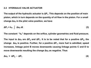
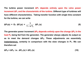
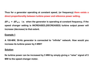
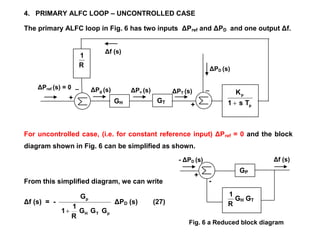
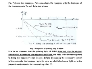
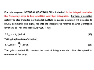
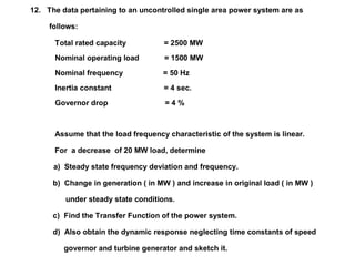
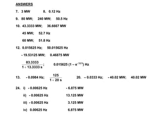
![Fig. 6 Block diagram corresponding to primary loop of ALFC
Power system
ΔPref (s)
Δf (s)
+
_
ΔPg (s) ΔPv (s) ΔPT (s)
+
_
ΔPD (s)
ΔPT (s) - ΔPD (s)
Δf (s) = Gp (s) [ ΔPT(s) – ΔPD(s) ] (22)
where
Gp (s) =
D
s
f
H
2
1
0
=
D
f
2H
s
1
1/D
0
=
p
p
T
s
1
K
(23)
Kp =
D
1
(24) Tp =
D
f
H
2
0
(25)
Equation (22) represents the missing link in the control loop of Fig. 4. By
adding this, block diagram of the primary ALFC loop is obtained as shown in
Fig. 6.
R
1
GH GT
p
p
T
s
1
K
](https://image.slidesharecdn.com/alfc-230523014933-24458dcc/85/ALFC-pdf-29-320.jpg)
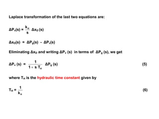
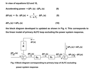
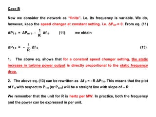
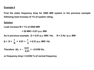
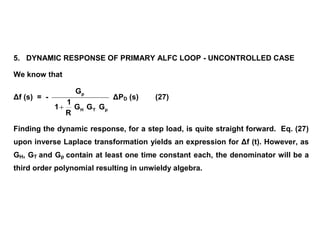
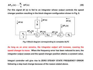
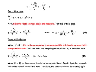
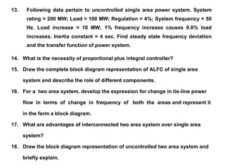
![4.1 STATIC FREQUENCY DROP DUE TO STEP LOAD CHANGE
For a step load change of constant magnitude ΔPD = M, we have ΔPD (s) =
s
M
Using the final value theorem, we readily obtain from eq. (27),
Δf (s) = -
p
T
H
p
G
G
G
R
1
1
G
ΔPD (s) (27) the static frequency drop as
Δf0 = [ s Δf (s) ] = -
R
K
1
K
p
p
M = -
R
1
D
M
Hz (28)
We introduce here the so-called Area Frequency Response Characteristic (AFRC)
β, defined as
β = D +
R
1
p.u. MW / Hz (29)
Then the static frequency drop is given by
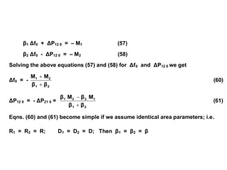
Δf0 = -
β
M
Hz (30)
lim
s 0](https://image.slidesharecdn.com/alfc-230523014933-24458dcc/85/ALFC-pdf-32-320.jpg)
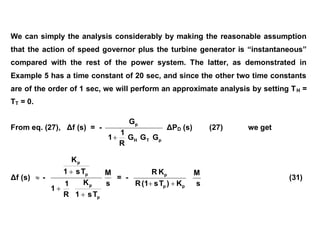
![Δf (s) = -
p
p
T
s
1
K
ΔPD(s)
ΔPref (s)
Δf (s)
+
_
ΔPg (s) ΔPv (s) ΔPT (s)
+
_
ΔPD (s)
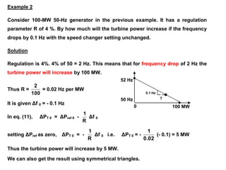
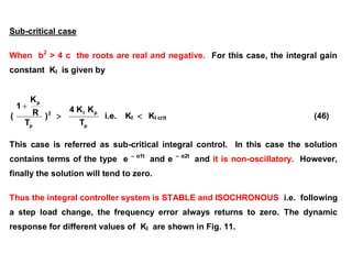
Example 7
What would the frequency drop in the previous example if the speed-governor
loop were non-existent or open?
Solution
ALFC loop reduces to
For a sudden load increase of M, ΔPD (s) =
s
M
Then Δf0 = [ s Δf (s) ] = - Kp M = -
D
M
Hz; Thus β = D = 0.01 p.u. MW / Hz
Therefore Δf0 = -
0.01
0.01
= - 1.0 Hz; or frequency drop = 2 % of normal frequency
lim
s 0
Δf (s)
- ΔPD (s)
p
p
T
s
1
K
R
1
GH GT
p
p
T
s
1
K
](https://image.slidesharecdn.com/alfc-230523014933-24458dcc/85/ALFC-pdf-34-320.jpg)
![Δf (s) -
s
M
T
s
1
K
R
1
1
T
s
1
K
p
p
p
p
= -
p
p
p
K
)
T
s
(1
R
K
R
s
M
(31)
Dividing numerator and denominator by R Tp we get
Δf(s) = -
p
p
T
K
M
)
p
p
T
R
K
R
s
(
s
1
(32)
Using the fact
)
α
(s
s
A
=
α
A
[
s
1
-
α
s
1
] and noting
p
p
p
p
p
p
K
R
K
R
M
K
R
T
R
T
K
M
α
A
equation (32) becomes
Δf(s) = - M
p
p
K
R
K
R
[
s
1
-
p
p
T
R
K
R
s
1
] (33)](https://image.slidesharecdn.com/alfc-230523014933-24458dcc/85/ALFC-pdf-37-320.jpg)
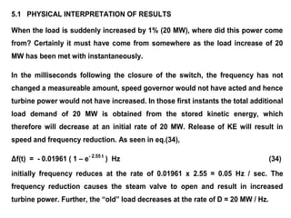
![Δf(s) = - M
p
p
K
R
K
R
[
s
1
-
p
p
T
R
K
R
s
1
] (33)
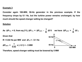
Making use of previous numerical values: M = 0.01 p.u. MW; R = 2.0 Hz / p.u. MW;
Kp = 100 Hz / p.u. MW; Tp = 20 sec.
M
p
p
K
R
K
R
=
102
2
= 0.01961;
p
p
T
R
K
R
=
40
102
= 2.55
Δf(s) = - 0.01961 [
s
1
-
2.55
s
1
]
The approximate time response is purely exponential and is given by
Δf(t) = - 0.01961 ( 1 – e- 2.55 t
) Hz (34)](https://image.slidesharecdn.com/alfc-230523014933-24458dcc/85/ALFC-pdf-38-320.jpg)
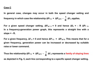
![Fig. 6 a Reduced block diagram
Δf (s)
- ΔPD (s)
+
-
Δf (s)
+
-
s
0.01
Alternatively, the above result can be obtained from the reduced block diagram
shown in Fig. 6 a . Then
Thus Δf(s) = -
2.55)
(s
s
0.05
51)
s
(20
s
1
s
0.01
50
s
20
1
100
s
0.01
s
20
1
50
1
s
20
1
100
= ]
2.55
s
1
s
1
[
0.01961
]
2.55
s
1
s
1
[
2.55
0.05
Δf(t) = - 0.01961 ( 1 – e- 2.55 t
) Hz (34)
GP
R
1
GH GT
s
20
1
100
0.5](https://image.slidesharecdn.com/alfc-230523014933-24458dcc/85/ALFC-pdf-39-320.jpg)
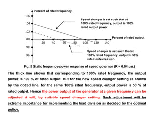
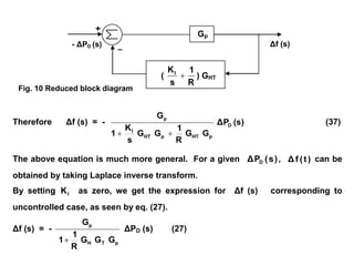
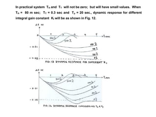
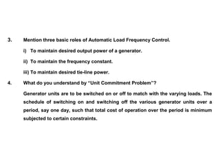
![Fig. 9 Reduced block diagram
Fig. 10 Reduced block diagram
_ Δf (s)
+
- ΔPD (s)
Referring to the block diagram of single control area with integral controller
shown in Fig. 8, input to T
H
G is - )
s
(
f
Δ
s
KI
-
R
1
Δf (s) i.e.
- [
s
KI
+
R
1
] Δf (s). Using this, the block diagram in Fig. 8 can be reduced as
shown in Fig. 9 and 10.
Gp
(
R
1
s
KI
) GHT
ΔPT (s)
+
_
ΔPD (s)
Δf (s)
GHT Gp
- (
R
1
s
KI
)](https://image.slidesharecdn.com/alfc-230523014933-24458dcc/85/ALFC-pdf-46-320.jpg)
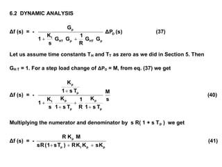
![Δf (s) = - (s)
ΔP
G
G
R
1
G
G
s
K
1
G
D
p
HT
p
HT
I
p
(37)
6.1 STATIC FREQUENCY DROP FOLLOWING A STEP LOAD CHANGE
Let the step load change be ΔPD, which is equal to M. Then ΔPD(s) =
s
M
Using final value theorem,
Δf0 = [ s Δf (s) ] (38)
= -
p
HT
p
HT
I
p
G
G
R
1
G
G
s
K
1
M
G
= -
p
p
I
p
K
R
1
K
s
K
1
M
K
= 0 (39)
Thus static frequency drop due to step load change becomes zero, which is a
desired feature we were looking. This is made possible because of the integral
controller that has been introduced.
lim
s 0
s 0 s 0](https://image.slidesharecdn.com/alfc-230523014933-24458dcc/85/ALFC-pdf-48-320.jpg)
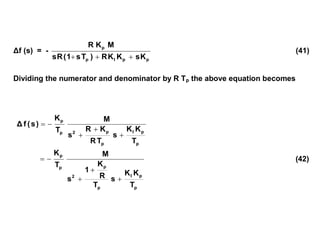
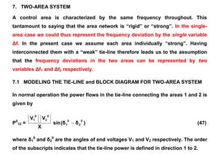
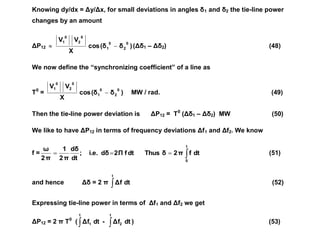
![Fig. 13 Representation of Tie-lone power flow
_
+ ΔP12 (s)
Δf1 (s)
Δf2 (s)
ΔP12 = 2 π T0 (
t
1 dt
Δf -
t
2 dt
Δf ) (53)
Taking Laplace transformation of the above eq. we get
ΔP12(s) =
s
T
π
2 0
[ Δf1 (s) – Δf2 (s) ] (54)
Representing this equation in terms of block diagram symbols yields the diagram
in Fig. 13.
Tie-line power ΔP12 shall be treated as load in area 1. Similar to power balance eq.
Δf (s) = Gp (s) [ ΔPT(s) – ΔPD(s) ] (22) we can write
Δf1 (s) = Gp1 (s) [ ΔPT1(s) – ΔPD1(s) – ΔP12(s)] (54 a)
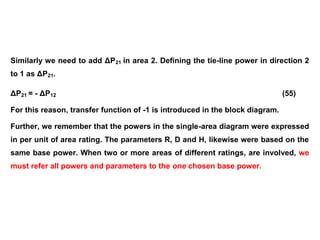
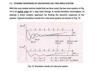
Block diagram for two-area uncontrolled system is shown in Fig. 14.
2 π T0
s
1](https://image.slidesharecdn.com/alfc-230523014933-24458dcc/85/ALFC-pdf-57-320.jpg)
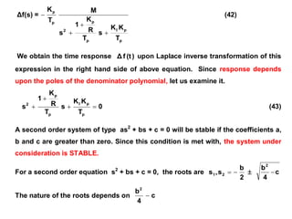
![Fig. 14 Block diagram representation of two area system
ΔPref 1 (s) ΔPT1 (s)
+
_
ΔPD1 (s)
Δf1 (s)
+
_
ΔPg1 (s)
Δf1 (s)
ΔPref 2 (s) ΔPT2 (s)
+ _
ΔPD2 (s)
+
_
ΔPg2 (s)
Δf2 (s)
+
_
Δf2 (s)
ΔP12 (s)
ΔP21 (s)
_
_
Δf1 (s) = Gp1 (s) [ ΔPT1(s) – ΔPD1(s) – ΔP12(s)] (54 a)
1
R
1
GHT1 Gp1
GHT2 Gp2
2
R
1
2πT0
s
1
-1](https://image.slidesharecdn.com/alfc-230523014933-24458dcc/85/ALFC-pdf-58-320.jpg)

![But this evidently requires that both the integrants in eqns (68) and (69) be zero;
i.e.
ΔP12 0 + B1 Δf 0 = 0 (70)
and ΔP21 0 + B2 Δf 0 = 0 i.e. - ΔP12 0 + B2 Δf 0 = 0 (71)
The above two conditions can be met with only if
Δf 0 = 0 and ΔP21 0 = - ΔP12 0 = 0 (72)
Note that this result is independent of the values of B1 and B2. In fact, one of the
bias parameters can be zero, and we still have a guarantee that eq. (72) is
satisfied. Having checked use of the integral controller, let us see how they can be
included in the block diagram.
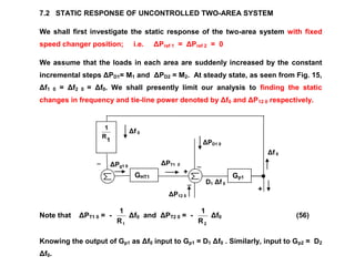
Laplace transform of Equations (68) and (69) gives
ΔPref 1 (s) =
s
I1
K
[ΔP12 (s) + B1 Δf1 (s)]; ΔPref 2 (s) =
s
I2
K
[ΔP21 (s) + B2 Δf2 (s)]](https://image.slidesharecdn.com/alfc-230523014933-24458dcc/85/ALFC-pdf-70-320.jpg)
![ΔPT1 (s)
+
_
ΔPD1 (s)
Δf1 (s)
+
_
ΔPg1 (s)
Δf1 (s)
ΔPref 2 (s) ΔPT2 (s)
+ _
ΔPD2 (s)
+
_
ΔPg2 (s)
Δf2 (s)
+
_
Δf2 (s)
ΔP12 (s)
ΔP21 (s)
_
_
ΔPref 1 (s)
ΔP12 (s)
ΔP12 (s)
ΔP21 (s)
Δf1 (s)
Δf2 (s)
+
+
+
+
Fig. 16 Block diagram representation of two area system with tie-line bias control
ΔPref 1 (s) =
s
I1
K
[ΔP12 (s) + B1 Δf1 (s)]; ΔPref 2 (s) =
s
I2
K
[ΔP21 (s) + B2 Δf2 (s)]
s
K 1
I
1
R
1
GHT1 Gp1
GHT2 Gp2
2
R
1
2πT0
s
1
-1
-1
B1
B2
s
K 2
I
](https://image.slidesharecdn.com/alfc-230523014933-24458dcc/85/ALFC-pdf-71-320.jpg)

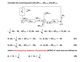
![Δf (s)
- ΔPD (s)
+
-
ΔPref (s)
+
_
ΔPg (s) ΔPv (s) ΔPT (s)
+
_
ΔPD (s)
This can be reduced as
Thus Δf (s) = -
p
G
T
G
H
G
R
1
1
p
G
ΔPD (s)
Let ΔPD = M ; Then ΔPD(s) =
s
M
and hence
Δf (s) = -
p
T
H
p
G
G
G
R
1
1
G
s
M
Using the final value theorem, the static frequency drop is
Δf0 = [ s Δf (s) ] = -
R
p
K
1
p
K
M = -
R
1
D
M
Hz
lim
s 0
GP
R
1
GH GT
R
1
GH GT
p
p
T
s
1
K
](https://image.slidesharecdn.com/alfc-230523014933-24458dcc/85/ALFC-pdf-87-320.jpg)