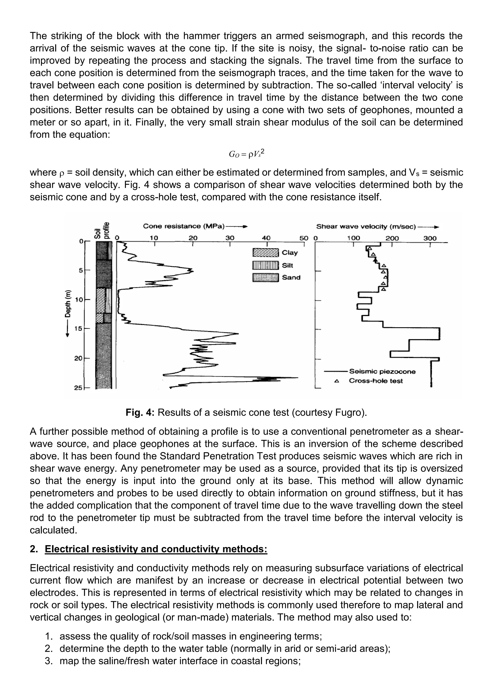
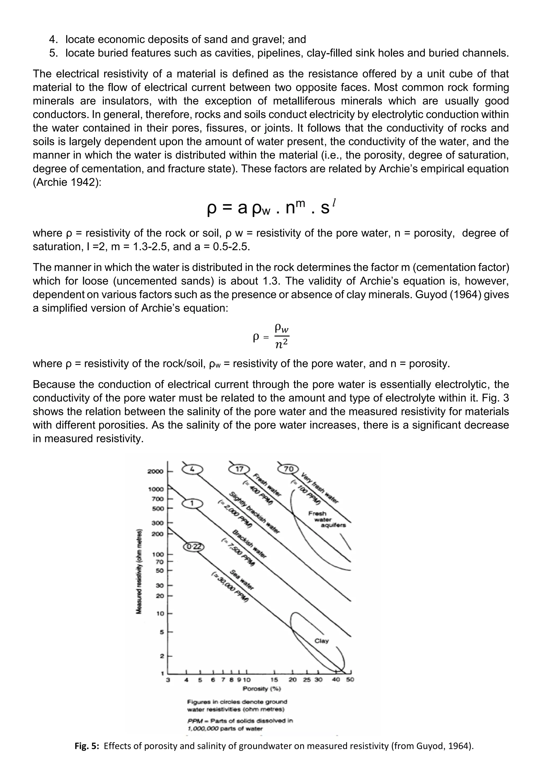
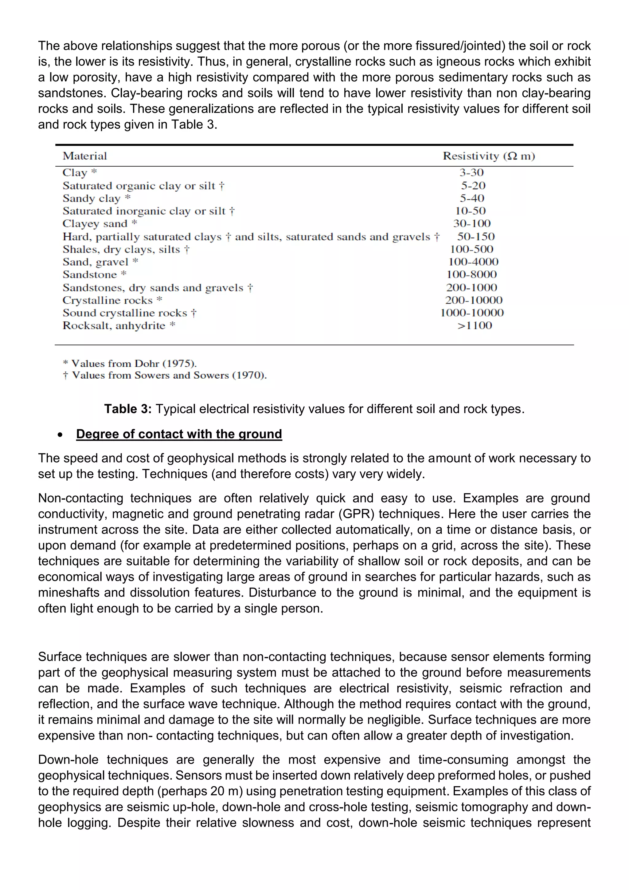
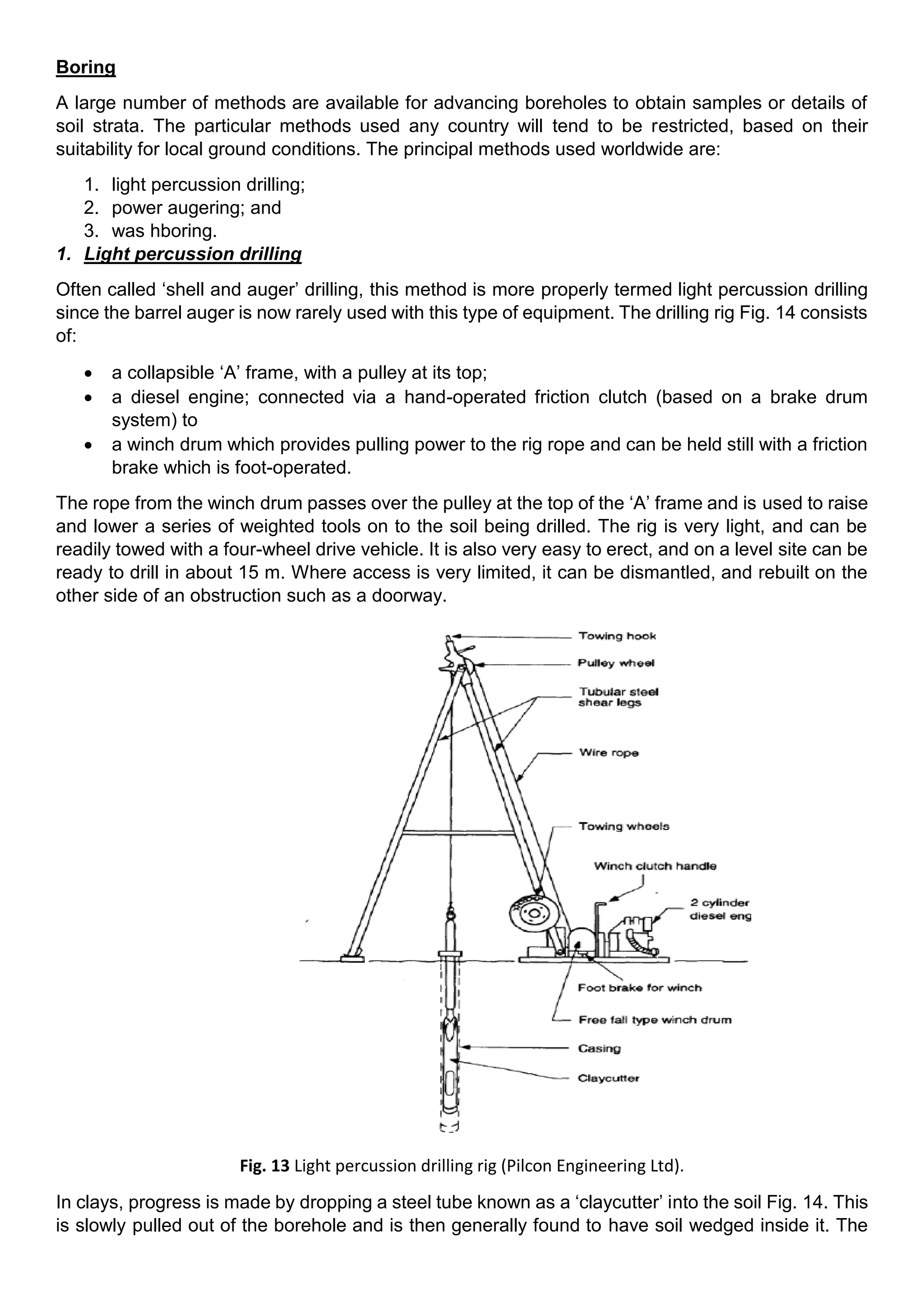
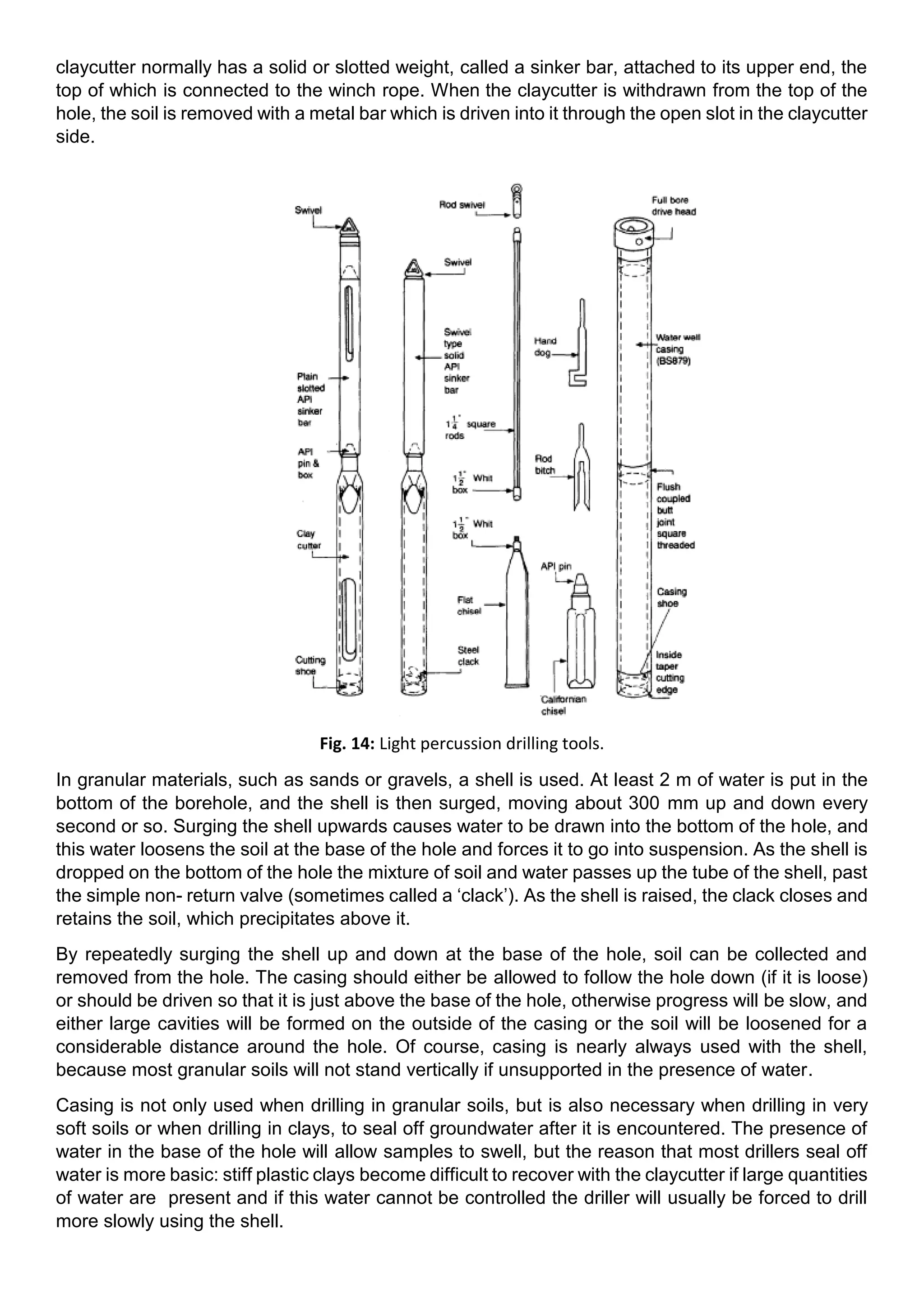
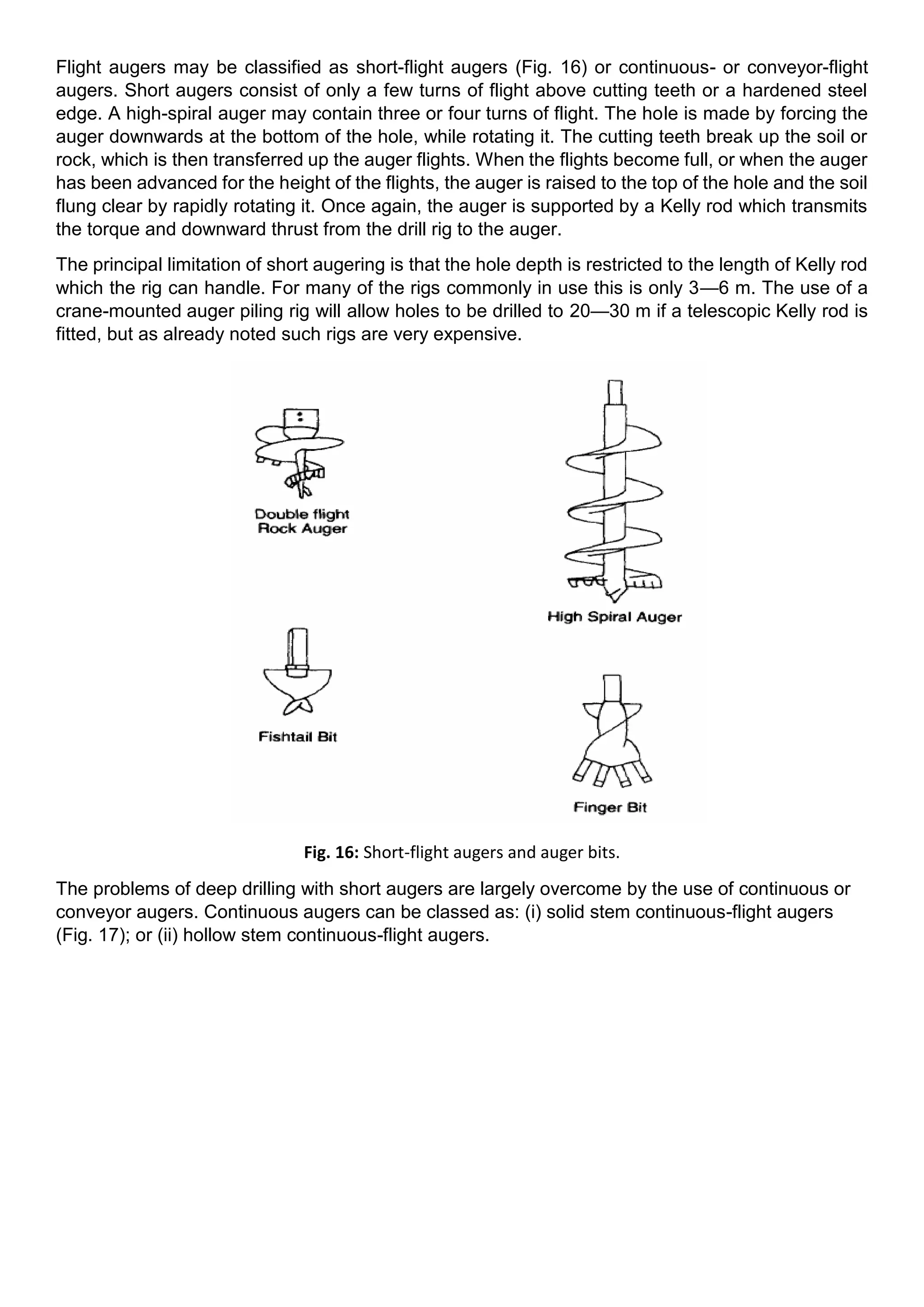
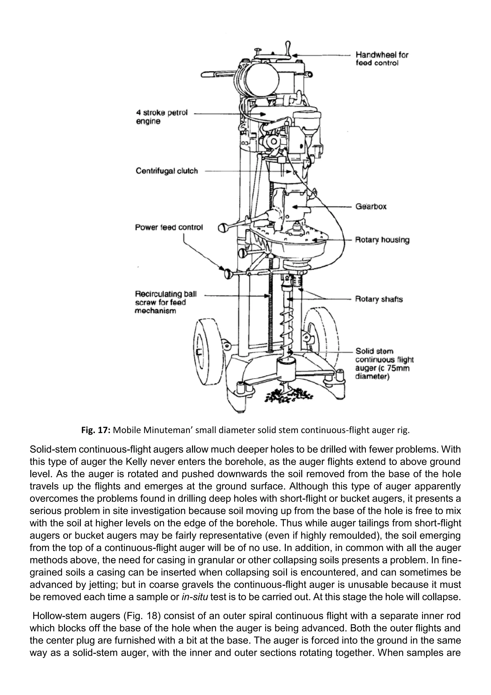
Geotechnical site investigation

Geotechnical Site Investigation.
By
Abd Al Rahman Ibrahim Ahmed Mohamed
BSc. Geology/ Geophysics,
Faculty of Science, Alexandria University
Abdalrahmanibrahim209@gmail.com
Supervised by: Prof. Dr. Mohamed A. Rashed
Geology Department
Faculty of Science, Alexandria university

Contents:
• Introduction
• History and development
• General design philosophy
• Approaches to site investigation
o Approach 1: Desk-study and geotechnical advice
o Approach 2: ‘Standard’ ground investigation
o Approach 3: Limited investigation, coupled with monitoring
o Approach 4: The observational method
• The sequence of geotechnical site investigation might be
• Planning ground investigations
• Planning trial pitting, boring and drilling
• Borehole layout and frequency
• Depth of borings
• Subsurface exploration: engineering geophysics
• Classification of geophysical techniques
o Passive techniques
o Active techniques
• Types of measurement
• Seismic Method
o Seismic profiling
• Electrical resistivity and conductivity methods
o Electrical resistivity traversing
o Electrical resistivity sounding
• Gravity methods
• Subsurface exploration: boring, drilling, probing and trial pitting
o Boring
o Light percussion drilling
o Augering
o Washboring
• Drilling
o Open-holing
o Coring
o Coring equipment
o Bits
o Flush fluid
▪ Air
▪ Water
▪ Bentonite and polymer muds
o Drill hole testing
▪ Orientation
▪ Borehole impression packer

• In situ Testing
o Introduction
1. penetration resistance
a. The Standard Penetration Test (SPT)
b. The cone penetration test (CPT)
i. Mechanical cone testing
ii. Electric cone testing
iii. The piezocone
iv. The seismic cone
2. strength and/or compressibility
a. The field vane test.
b. The pressure-meter test.
c. The plate loading test
d. The Marchetti dilatometer.
3. in situ permeability
a. rising and falling head tests;
b. constant head tests; and
c. packer or Lugeon tests.

Geotechnical Site Investigation and Laboratory Testing.
Introduction:
Geotechnical engineering, as the name implies, concerns the applications of civil engineering
technology to some aspect of the earth. Usually, the geotechnical engineer is concerned only with
the natural materials found at or near the surface of the earth.
Civil engineers call these earthen materials soil and rock. Soil, in an engineering sense, is the
relatively loose agglomerate of mineral and organic materials and sediments found above the
bedrock. Soils can be relatively easily broken down into their constituent mineral or organic particles.
Rocks, on the other hand, have very strong internal cohesive and molecular forces which hold the
constituent mineral grains together. This is true whether the rock is massive bedrock or a piece of
gravel found in a clay soil.
The dividing line between soil and rock is arbitrary, and many natural materials encountered in
engineering. practice cannot be easily classified. They may be either "a very soft rock" or "a very
hard soil." Other scientific disciplines have different meanings for the terms soil and rock. In
geology, for example, rock means all the materials found in the earth's crust, independently of how
much the mineral particles are bound together. Soils to a geologist are just decomposed and
disintegrated rocks generally found in the very thin upper part of the crust and capable of supporting
plant life. Similarly, pedology (soil science) and agronomy are concerned with only the very
uppermost layers of soil, that is, those materials relating to agriculture and forestry. Geotechnical
engineers can learn much from both geology and pedology. Both sciences, especially engineering
geology, are important adjuncts to geotechnical engineering and there is considerable overlap
between these fields. But differences in terminology, approach, and objectives may cause some
confusion, especially for the beginner.
Geotechnical engineering has several different aspects or emphases. Soil mechanics is the branch
of geotechnical engineering concerned with the engineering mechanics and properties of soil,
whereas rock mechanics is concerned with the engineering mechanics and properties of rock,
usually but not necessarily the bedrock. Soil mechanics applies the basic principles of mechanics
including kinematics, dynamics, fluid mechanics, and the mechanics of materials to soils. In other
words, soil rather than water or steel or concrete, for example, now becomes the engineering
material whose properties and behavior we must understand in order to build with it or upon it. A
similar comment could also be made for rock mechanics.
It should be noted, however, that there are significant differences between the behavior of soil
masses and rock masses, and in principle there is not much overlap between the two disciplines.
• Foundation engineering applies geology, soil mechanics, rock mechanics, and structural
engineering to the design and construction of foundations for civil engineering and other
structures. The foundation engineer must be able to predict the performance or response of
the foundation soil or rock to the loads imposed by the structure. Some examples of the kinds
of problems faced by the foundation engineer include foundations for industrial, commercial,
and residential buildings, and other types of support structures for radar towers, as well as
foundations for oil and other kinds of tanks and offshore structures. Even ships must have a
dry dock during construction or repairs, and the dry dock must have a foundation. The support
of rockets and appurtenant structures during construction and launch have led to very
interesting and challenging foundation engineering problems.

• Related geotechnical engineering problems facing the foundation engineer are the stability
of natural and excavated slopes, the stability of permanent and temporary earth-retaining
structures, problems of construction, controlling water movement and pressures, and even
the maintenance and rehabilitation of old buildings. Not only must the foundation safely
support the static structural and construction loads, but it must also adequately resist dynamic
loads due to blasting, earthquakes, etc..
If you think about it, it is impossible to design or construct any civil engineering structure without
ultimately considering the foundation soils and rocks to some extent, and this is true whether the
structure is built on the earth or is extraterrestrial. The performance, economy, and safety of any
civil engineering structure ultimately is affected or may even be controlled by its foundation.
Earth materials are often used as a construction material because they are the cheapest possible
building material. However, its engineering properties such as strength and compressibility are often
naturally poor, and measures must be taken to density, strengthen, or otherwise stabilize and
reinforce soils so that they will perform satisfactorily in service.
History and development:
Site investigation is the process by which geological, geotechnical, and other relevant information
which might affect the construction or performance of a civil engineering or building project is
acquired.
Soil and rock are created by many processes out of a wide variety of materials. Because deposition
is irregular, soils and rocks are notoriously variable, and often have properties which are undesirable
from the point of view of a proposed structure. Unfortunately, the decision to develop a particular
site cannot often be made on the basis of its complete suitability from the engineering viewpoint;
geotechnical problems therefore occur and require geotechnical parameters for their solution.
Site investigation will often be carried out by specialists in the field of soil mechanics. Soil, in the
engineering sense, is the relatively soft and uncemented material which overlies the rock of the
outer part of the Earth’s crust. Specialists in the mechanical behavior of soil are normally civil
engineers and in the UK they will often have some postgraduate geotechnical education: such
people are termed ‘soils engineers’ or ‘geotechnical engineers’.
Geologists with an interest in the relevance of geology to civil engineering or building construction
are called ‘engineering geologists.’
Soil mechanics in its present form is a relatively recent addition to the field of engineering. Interest
in the behavior of earth and rock for engineering purposes can be traced back to Roman times
(Palladius
in Plommer (1973)), but significant advances in analysis seem to date back to the eighteenth
century, when the need for large defensive revetments led to early work on retaining walls.
Coulomb’s paper, delivered to the Académie Royale des Sciences in 1773 and published in 1776,
represents an early work which showed considerable understanding, inter alia, of the behavior of
soil, and whose results are still valid and in use (Heyman 1972). Subsequent papers, principally
delivered by the French, did much to refine the available solutions but little to increase fundamental
knowledge.
By the first quarter of the nineteenth century, it appears that many concepts now associated with
the principle of effective stress were intuitively understood. Telford used pre-loading during the
construction of the Caledonian Canal in 1809 ‘for the purpose of squeezing out the water and
consolidating the mud’, and Stephenson used drains to lower pore pressures during the construction
of the Chat Moss embankment on the Liverpool and Manchester Railway in the years 1826 to 1829
‘in order to consolidate the ground between them on which the road was to be formed’ (Smiles

1874). During the industrial period preceding the twentieth century, many of the currently used
geotechnical processes for the improvement of ground, such as piling, pre-loading, compaction and
de-watering appear to have been used. These techniques were applied in a purely empirical
manner.
At the turn of the twentieth century, a series of major failures occurred which led to the almost
simultaneous formation of geotechnical research groups in various countries. In America, slope
failures on the Panama Canal led to the formation of the American Foundations Committee of the
American Society of Civil Engineers in 1913 and, in Sweden, landslides during a railway construction
resulted in the formation of the State Geotechnical Commission in the same year. Following a
number of embankment and dyke failures, a government committee under Buisman was set up in
Holland in 1920. Casagrande (1960), however, dates the advent of modern soil mechanics to the
period between 1921 and 1925, when Terzaghi published several important papers relating to the
pore pressures set up in clay during loading, and their dissipation during consolidation,
Terzaghi’s first professional work in England was in 1939, when he was retained to investigate a
slope failure at the Chingford reservoir. As a result, the first commercial soil mechanics laboratory
in the UK was established by John Mowlem and became Soil Mechanics Ltd in 1943 .Whyte (1976)
reports that by 1948 five other contractors and one consultant had soils divisions.
Major encouragement was given to soils research in the UK by Cooling, who influenced a number
of engineers (for example Skempton, Bishop and Golder) who worked at the Building Research
Station in the 1940s. In 1948, Géotechnique commenced publication, and by 1955 a great number
of significant papers on soil mechanics had been published covering topics such as site
investigation, seepage, slope stability and settlement.
According to Mayniel (1808), Bullet was the first to try to establish an earth pressure theory, in 1691.
More importantly from our point of view, Bullet notes the importance of site investigation for the
foundations of earth-retaining structures and recommends the use of trial holes in order to determine
the different beds of soil beneath a site, and in order to ensure that poor soil does not underlie good
soil. Where trial holes could not be made, Bullet recommended the use of an indirect method of
investigation whereby the quality of the soil was determined from the sound and penetration
achieved when it was beaten with a 6—8 ft length of rafter.
In 1949, the first draft Civil Engineering Code of Practice for Site Investigations was issued for
comment. At that time Harding (1949) delivered a paper to the Works Construction Division of the
Institution of Civil Engineers in which he detailed the methods of boring and sampling then available.
The recommendations made in that paper, and in discussions on the paper by Skempton, Toms
and Rodin form the basis of the majority of techniques still in use in site investigation in the United
Kingdom. For example, in his discussion on methods of boring, Harding notes that:
• the boring equipment used in site investigations is criticized by some who have not been
exposed to the need to carry it themselves, as being primitive and lacking in mechanization.
Whilst it is possible to think of many ingenious contrivances for removing articles at depths
below ground, in practice simple methods usually prove to be more reliable.
while Skempton confirmed this view:
• with that simple equipment [shell and auger gear and 102 mm dia. sampler] the majority of
site investigations in soils could be carried out and, moreover, sufficient experience was now
available to enable the positive statement to be made that, in most cases, the results obtained
by that technique (in association with laboratory tests) were sufficiently reliable for practical
engineering purposes.

By 1953, Terzaghi stated in connection with site investigation that ‘we have acquired all the
knowledge which is needed for a rational interpretation of the observational and experimental data.’
The reader may reasonably ask what is to be gained from this book, since techniques are so well
established. In reality, since 1950, four main changes have taken place. First, many of the methods
introduced before and since have been the object of criticism as a result of differences between
predictions and subsequent observations. Secondly, a considerable number of the lessons learnt
before 1950 have been forgotten: few U100 samplers in use today are of the standard required by
Hvorslev (1949)for undisturbed sampling, and much fieldwork remains unsupervised by engineers.
Thirdly, few engineers have an experience or understanding of the techniques of boring and drilling
holes for site investigations, and most clients remain unaware of the importance of this part of the
work. Finally, recent years have seen the introduction of sophisticated and expensive methods of
testing and computer analysis which cannot be sensibly applied to samples and predictions of soil
conditions of indeterminate quality.
The Civil Engineering Code of Practice No. 1: Site Investigations was issued in 1950, and revised
as British Standard Code of Practice CP 2001 in 1957. This code has now been extended,
completely rewritten and re-issued as British Standard 5930:1 981. At the time of writing (1992) BS
5930 is under revision. The code contains much valuable information, but it is perhaps necessary
to ask whether it is wise to codify in this way. Terzaghi (1951) argued that: since there is an infinite
variety of subsoil patterns and conditions of saturation, the use of the different methods of subsoil
exploration cannot be standardized, but the methods themselves still leave a wide margin for
improvement, as far as expediency and reliability are concerned.
General design philosophy:
Site investigation should be an integral part of the construction process. Unfortunately it is often
seen as a necessary evil a process which must be gone through by a designer if he or she is to
avoid being thought incompetent, but one which gives little of value and takes precious time and
money. This is an unfortunate by-product of the way in which site investigation is often carried out,
and it can hardly be surprising that if no effort is put into targeting the investigation to precise issues,
then little of value emerges.
Approaches to site investigation:
Approach 1: Desk-study and geotechnical advice
The minimum requirement for a satisfactory investigation is that a desk study and walk-over survey
are carried out by a competent geotechnical specialist, who has been carefully briefed by the lead
technical construction professional (architect, engineer or quantity surveyor) as to the forms and
locations of construction anticipated at the site.
This approach will be satisfactory where routine construction is being carried out in well-known and
relatively uniform ground conditions. The desk study and walk-over survey are intended to:
1. confirm the presence of the anticipated ground conditions, as a result of the examination of
geological maps and previous ground investigation records;
2. establish that the variability of the sub-soil is likely to be small;
3. identify potential construction problems;
4. establish the geotechnical limit states (for example, slope instability, excessive foundation
settlement) which must be designed for; and above all, to
5. investigate the likelihood of unexpected’ hazards (for example, made ground, or
contaminated land).
It is unlikely that detailed geotechnical design parameters will be required, since the performance of
the proposed development can be judged on the basis of previous construction.

Approach 2: ‘Standard’ ground investigation
For most projects a more elaborate approach is needed, and will generally follow the following
course.
1. A desk study and walk-over survey must first be carried out, to establish the likely conditions
on and below the site, as described above.
2. The details of the proposed construction must be ascertained, in as much as they have been
decided. Particular care should be taken to establish the probable loading conditions and the
sensitivity of any structures to be built, or those already existing on, around or below the site,
to the changes that will occur as a result of construction. For example, services and tunnels
passing below or alongside a proposed excavation for a basement may be damaged by the
movements caused by excavation, and buildings above a proposed tunnel may be damaged
by changes in the groundwater conditions and any ground loss caused by construction.
3. From the combinations of construction and ground conditions, the need for particular
foundation types, for retaining walls, for cut slopes, and for special construction processes
(such a grouting, dewatering and ground improvement) should be determined. These will
bring with them particular limit states, and where limit states cannot be avoided (for example,
by changing the configuration of the proposed construction) there will be a need to carry out
geotechnical analyses.
Example: potential limit states:
• Bearing capacity failure of foundations
• Differential settlement of foundations leading to structural damage
• Instability of clay slopes
• Sulphate attack on concrete
• Damage by mining subsidence
• Damage to surrounding structures as a result of excavating or dewatering an
excavation
• Ground collapse over pre-existing natural solution features
• Collapse of excavations as a result of excessive water inflow
The identification of potential limit states is a matter of experience, education and pessimism.
‘Confidence may impress the Client, but it has little effect on the forces of nature’
At this stage critical parameters, essential to the successful completion of the project, must be
recognized.
Example: parameters required for the design of a foundation in clay:
• Bulk unit weight of clay
• Undrained strength of clay
• Compressibility of clay
• Variability of the above, both laterally and with depth
• Groundwater level
• Sulphate content of groundwater
• Acidity of groundwater.
4. From a knowledge of the probable ground conditions and the required parameters, the
geotechnical specialist should now identify all possible ways of determining the required
parameters. Many tests that might be used will only work satisfactorily in limited ground
conditions, so limiting the available choice. In principle, the parameters may be obtained:

• based on published data from other sites;
• based on previous site investigation data;
• back-analysis of performance of nearby construction
• back-analysis of observed performance during construction;
• laboratory testing on samples taken during ground investigation; and
• in situ testing during ground investigation.
In order to optimize the investigation, estimates of:
• relative accuracy;
• relative cost;
• availability, and
• relevance to the problem
should be assessed for each way of determining the parameters.
Approach 3: Limited investigation, coupled with monitoring
In some projects, it may be possible to carry out redesign during construction, in order to reduce
costs. Given the natural variability of the ground, geotechnical engineers routinely use ‘moderately
conservative’ soil parameters in design calculations, and do not normally attempt genuine
predictions of values such as settlement, ground movements adjacent to excavations, etc. The
example below illustrates how the demolition and reconstruction process was modified during
construction, on the basis of moderately conservative design using finite element and boundary
element analysis, and observations of ground movements.
Approach 4: The observational method
This is a carefully considered approach to geotechnical design, developed by Peck (1969). Peck
(1969) ascribed Terzaghi’s great success to his use of observation, coupled with his insistence on
full, personal responsibility and authority on critical jobs. Clearly variations in financial constraints,
the complexity of soil conditions, and time restrictions mean that very different approaches can be
taken during site investigation. Peck argued that the methods available for coping with the inevitable
uncertainties which arise as a result of the natural variability of soil and rock conditions broadly form
three groups.
Method 1: Carry out limited investigation, and adopt an excessive factor of safety during design.
Method 2: Carry out limited investigation, and make design assumptions in accordance with general
average experience.
Method 3: Carry out very detailed investigation.
In the first two methods only the vaguest approximations to the values of the physical properties of
the sub-soil can be obtained. The variability of the soil properties, together with the degree of
continuity of the individual layers of soil are almost certainly unknown, and groundwater conditions
will not usually be adequately defined. Under these conditions it is almost certain that method 1 will
be wasteful, while method 2 can frequently be dangerous. Only in the cases of investigations of
major projects is there any likelihood that sufficient funds will be available for very detailed
investigations, and in many cases the financial return will not merit this approach. Peck (1969) gives
the ingredients of the ‘observational method’ as follows:
1. exploration sufficient to establish at least the general nature, pattern and properties of the
deposits, but not necessarily in detail;
2. assessment of the most probable conditions and the most unfavorable conceivable
deviations from these conditions. In this assessment geology often plays a major role;

3. establishment of the design based on a working hypothesis of behavior anticipated under the
most probable conditions;
4. selection of quantities to be observed as construction proceeds, and calculation of their
anticipated values on the basis of the working hypothesis;
5. calculation of values of the same quantities under the most unfavorable conditions compatible
with the available data concerning the subsurface conditions;
6. selection in advance of a course of action or modification of design for every foreseeable
significant deviation of the observational findings from those predicted on the basis of the
working hypothesis;
7. measurement of quantities to be observed and evaluation of actual conditions during
construction; and
8. modification of the design to suit actual conditions.
The sequence of geotechnical site investigation might be:
1. preliminary desk study, or fact-finding survey;
2. air photograph interpretation;
3. site walk-over survey;
4. preliminary subsurface exploration;
5. soil classification by description and simple testing;
6. detailed subsurface exploration and field testing;
7. the physical survey (laboratory testing);
8. evaluation of data;
9. geotechnical design;
10. field trials; and
11.liaison by geotechnical engineer with site staff during project construction
It has been found that the best site investigations involve a considerable number of activities, some
of which may become relatively unimportant in some cases, but should never be forgotten. An ideal
order of events might be as shown in Table 1.

Table 1. Order of events for site investigations
Planning ground investigations:
The process of all site investigation should be, above all, one of scientific method. Sufficient factual
information should be gathered (from the desk study and walk-over survey) to form hypotheses
regarding the ground conditions, and from this and a reasonable knowledge of what is to be built on
the site, the problems likely to be encountered both during the construction and the life of the
development must be predicted. The design of the proposed construction should then, ideally, take
into account the project’s geotechnical setting, in order to avoid as many difficulties as possible, and
minimize the remainder. Finally, ground investigation should be carried out in order, if necessary, to
determine the actual ground conditions on the site, and where necessary to obtain parameters for
engineering calculations.
Field investigation, whether by geophysics, or by boring or drilling, must have clearly identified aims
if it is to be worthwhile. In some situations it may be necessary to make extensive and detailed

ground investigations, but it is also perfectly conceivable that in other situations very few (if any) trial
pits or boreholes or soil testing will be required before the start of construction. At present, ground
investigation is poorly targeted, and it is because of this that it is sometimes regarded as a necessary
but rather unrewarding expense. Yet it must be remembered that the majority of unforseen costs
associated with construction are geotechnical in nature.
Because the planning of ground investigation is so important, it is essential that an experienced
geotechnical specialist is consulted by the promoter of the project and his leading technical designer
very early during conceptual design. The planning of a ground investigation is broken down into its
component parts in Table 2. The geotechnical specialist may be an independent consultant.
Table 2 Planning a ground investigation
Once a geotechnical specialist has been appointed, work can start on determining the ground
conditions at the site. The first stages of this process are the desk study, air photograph
interpretation, and a site walk-over survey. In geotechnical work, descriptions of soil and rock are
made in accordance with very specific guidelines (discussed below), which have been devised to
indicate their performance under engineering conditions, in terms of strength, compressibility and
permeability. If previous site investigation reports exist for construction in the same soil, this allows
the geotechnical engineer to judge (albeit in a general way) the likely performance of the ground
under and around the proposed development. In any case, geological maps coupled with experience
will give a considerable amount of information, of great value in the initial stages of design.
Planning trial pitting, boring and drilling:
Drilling and trial pitting are normally carried out for a number of reasons, such as:
1. to establish the general nature of the strata below a site;
2. to establish the vertical or lateral variability of soil conditions;
3. to verify the interpretation of geophysical surveys;
4. to obtain samples for laboratory testing;
5. to allow in situ tests to be carried out; and
6. .to install instruments such as piezometers, or extensometers.
Frequently, most if not all of these objectives will control the method of drilling on site. All the
objectives must be achieved with the minimum of expense and disruption to occupiers of the site.

The principal factors which allow a logical drilling program to be planned and successfully executed
are:
1. a relationship between structure, borehole layout, frequency and depth;
2. a need for sample quality and quantity related to the required geotechnical parameters and
the soil type and variability;
3. site supervision, to ensure that drilling and sampling are carried out to a high standard and
that good records are kept; and
4. prompt sample description and preparation of borehole and pit records in order that the
drilling program can be modified as the work proceeds.
These factors are considered in turn below.
Borehole layout and frequency:
Borehole layout and frequency are partly controlled by the complexity of the geological conditions.
The complexity of geological structure and the variability of each of the soil or rock units should be
at least partially known after the fact-finding or desk study. If soil conditions are relatively uniform,
or the geological data are limited, the following paragraphs will give an initial guide. Borehole layout
and frequency may need to be changed as more information emerges. Investigation will normally
be carried out by machine or hand-excavated trial pits, where only shallow depths are to be
investigated, for example for low-rise housing projects, or for shallow instability problems. The use
of pits in these situations allows a detailed engineering description of soil conditions, and will also
permit block samples to be taken. Most boreholes will be considerably deeper than can be
excavated by an open trial pit, and these will normally be carried out by light percussion or hollow
stem auger drilling.
Most projects will fall into one of the following categories:
1. isolated small structures, such as pylons, radio masts, or small houses, where one borehole
may be sufficient;
2. compact projects, such as buildings, dams, bridges or small landslips, will require at least
four boreholes. These will normally be deep and relatively closely spaced;
3. extended projects, such as motorways, railways, reservoirs and land reclamation schemes
will require shallower, more widely spaced boreholes, but these will normally be expected to
verify the depth of ‘good’ ground. In the case of road projects this will mean either rock head,
or a soil with a ‘stiff’ consistency. In the case of reservoirs, borings should be continued until
an adequate thickness of impermeable ground is found.
The frequency of borings on extended sites must be judged on the basis of the uniformity or
otherwise of the site geology and its expected soil variability. On a highway project the
recommendations for borehole spacing vary from 30 to 60 m to 160 m in changeable soils and 300m
in uniform soils.
Many projects, such as highways, are a combination of the categories described above. Structures
on extended projects should be treated as compact projects. For example, a typical investigation for
a motorway in the UK might use 5: 10 m deep borings every 150 m along the proposed road line,
with four 25: 30 m deep borings at the proposed position of each bridge structure. Additional
boreholes might be placed on the basis of soil information found during the fact-finding survey, on
the basis of:
1. the geological succession in the area. Thin beds of limited outcrop may require closer
boreholes;
2. the presence of drift deposits such as alluvium or glacial till, whose vertical and lateral extent
may require close inspection;

3. problem areas, for example where pre-existing slope instability is suspected.
The layout of the borings should aim not only to provide soil profiles and samples at positions related
to the proposed structures and their foundations, but should also be arranged to allow the
hypotheses formed during the fact-finding survey to be checked. The borings should be positioned
to check the geological succession and to define the extent of the various materials on site, and they
should be aligned, wherever possible, in order to allow cross-sections to be drawn (Fig. 1). Where
structures are to be found on slopes, the overall stability of the structure and the slope must
obviously be investigated, and to this end a deep borehole near the top of the slope can be very
useful.
Fig. 1: Alignment of boreholes
Depth of borings:
It is good practice on any site to sink at least one deep borehole to establish the solid geology. On
extended projects several of these may be necessary, partly in order to establish the depth of
weathering, which may be up to 100 m below ground level and may be irregular, and also to
establish the depth to which cavernous or mined areas descend.
The borings should be extended to strata of adequate bearing capacity and should penetrate all
deposits which are unsuitable for foundation purposes such as unconsolidated fill, peat, organic silt
and very soft and compressible clay. The soft strata should be penetrated even when they are
covered with a surface layer of high bearing capacity.

When structures are to be founded on clay and other materials with adequate strength to support
the structure but subject to consolidation by an increase in the load, the borings should penetrate
the compressible strata or be extended to such a depth that the stress increase for still deeper strata
is reduced to values so small that the corresponding consolidation of these strata will not materially
influence the settlement of the proposed structure.
Except in the case of very heavy loads or when seepage or other considerations are governing, the
borings may be stopped when rock is encountered or after a short penetration into strata of
exceptional bearing capacity and stiffness, provided it is known from explorations in the vicinity or
the general stratigraphy of the area that these strata have adequate thickness or are underlain by
still stronger formations. When these conditions are not fulfilled, some of the borings must be
extended until it has been established that the strong strata have adequate thickness irrespective
of the character of the underlying material.
When the structure is to be founded on rock, it must be verified that bedrock and not boulders have
been encountered, and it is advisable to extend one or more borings from 10 to 20 ft. into solid rock
in order to determine the extent and character of the weathered zone of the rock. In regions where
rock or strata of exceptional bearing capacity are found at relatively shallow depths say from 100 to
150 ft. it is advisable to extend at least one of the borings to such strata, even when other
considerations may indicate that a smaller depth would be sufficient. The additional information
thereby obtained is valuable insurance against unexpected developments and against overlooking
foundation methods and types which may be more economical than those first considered. The
depth requirements should be reconsidered, when results of the first borings are available, and it is
often possible to reduce the depth of subsequent borings or to confine detailed and special
explorations to particular strata.
As a rough guide to the necessary depths, as determined from considerations of stress distribution
or seepage, the following depths may be used.
1. Reservoirs. Explore soil to: (i) the depth of the base of the impermeable stratum, or (ii) not
less than 2 x maximum hydraulic head expected.
2. Foundations. Explore soil to the depth to which it will be significantly stressed. This is often
taken as the depth at which the vertical total stress increase due to the foundation is equal to
10% of the stress applied at foundation level (Fig. 2).
3. For roads. Ground exploration need generally only proceed to 2: 4 m below the finished road
level, provided the vertical alignment is fixed. In practice some realignment often occurs in
cuttings, and side drains may be dug up to 6 m deep. If site investigation is to allow flexibility
in design, it is good practice to bore to at least 5 m below ground level where the finished
road level is near existing ground level, 5 m below finished road level in cut, or at least one
and-a half times the embankment height in fill areas.
4. For dams. For earth structures, recommends a depth equal to one-half of the base width of
the dam. For concrete structures the depth Of exploration should be between one-and-a-half
and two times the height of the dam. Because the critical factor is safety against seepage
and foundation failure, boreholes should penetrate not only soft or unstable materials, but
also permeable materials to such a depth that seepage patterns can be predicted.
5. For retaining walls. the preliminary depth of exploration should be three-quarters to one-and
a-half times the wall height below the bottom of the wall or its supporting piles. Because it is
rare that more than one survey will be carried out for a small structure, it will generally be
better to err on the safe side and bore to at least two times the probable wall height below
the base of the wall.
6. For embankments. The depth of exploration should be at least equal to the height of the
embankment and should ideally penetrate all soft soils if stability is to be investigated. If

settlements are critical then soil may be significantly stressed to depths below the bottom of
the embankment equal to the embankment width.
Fig. 2: Necessary borehole depths for foundations.

Subsurface exploration: engineering geophysics:
Geophysical techniques offer the chance to overcome some of the problems inherent in more
conventional ground investigation techniques. Many methods exist with the potential of providing
profiles and sections, so that (for example) the ground between boreholes can be checked to see
whether ground conditions at the boreholes are representative of those elsewhere. Geophysical
techniques also exist which can be of help in locating cavities, backfilled mineshafts, and dissolution
features in carbonate rocks, and there are other techniques which can be extremely useful in
determining the stiffness properties of the ground.
Yet, at the time of writing, geophysics is only rarely used in ground investigations. Various reasons
have been put forward to explain this fact, including:
1. poor plaAZZZZZZZZZZZnning of geophysical surveys, by engineers ignorant of the
techniques; and
2. over optimism by geophysicists, leading to a poor reputation for the available techniques.
Most geophysical techniques have as their origin the oil and mining industries. In such industries
the primary need of a developer is to identify the locations of minerals for exploitation, against a
background of relatively large financial rewards once such deposits are found. Geophysics plays a
vital role intermediate between geological interpretation of the ground and its structure, and the
drilling of exploratory holes to confirm the presence of ores, oil or gas. In most cases the minerals
are deep, and drilling is very expensive geophysics allows optimization of the drilling investigation,
amongst other things. Many mineral explorations will be centered upon deep deposits, where ground
conditions are spatially relatively uniform, and geological structures are large. Geophysical
techniques are relatively cheap, and are highly regarded in such a speculative environment, even
though they may not always be successful.
In contrast, ground investigations are carried out against a professional, contractual and legal
background which often demands relatively fine resolution and certainty of result. The idea that a
test or method will be successful and yield useful data only in a proportion of the cases in which it
is used is unacceptable. it is necessary for a geotechnical engineer to weigh carefully the need for
each element of his ground investigation. He will often have to persuade his client to provide
additional funds for nonstandard techniques, and if these are unsuccessful the client may not be
convinced of his competence. Therefore, when using geophysical techniques during ground
investigation, as part of the engineering design process, great care is needed. The engineer should
convince himself of the need for such a survey, and should take care of ensure that only appropriate
and properly designed surveys are carried out.
Unfortunately, there has been a widespread failure of geophysical techniques to perform as
expected during ground investigations.
❖ In selecting a particular geophysical technique for use on a given site, it is essential that the
following questions are asked.
1. What is the objective of the survey?
It is generally true that users of geophysics expect the survey to provide a number of types of
information. In fact, the converse is true. The survey should normally be designed to provide
information on a single aspect of the site. A number of examples are given below
• depth to rock head;
• position of old mineshafts;
• corrosivity of the ground;

• very small strain stiffness of the ground;
• extent of saline intrusion of groundwater;
• position of cohesive and granular deposits along a pipeline route.
2. What is the physical property to be measured?
Given the ‘target’ of the geophysical investigation, the physical property that is to be measured may
be obvious. For example, if the target is to be the determination of the very small strain stiffness of
the ground, then it follows that the property that must be measured is the seismic shear wave
velocity. But in many cases the success of a geophysical survey will depend upon the choice of the
best geophysical method, and the best geophysical method is likely to be the one which is most
sensitive to the variations in the ground properties associated with the target. For example, in trying
to locate a mineshaft it might be relevant to consider whether metallic debris (for example, winding
gear) has been left at the location (making magnetic methods likely to be successful) or whether the
shaft is empty and relatively close to the ground (making gravity methods attractive).
3. Which method is most suited to the geometry of the target?
Geophysical targets range from cavities to boundaries between rock types, and from measurements
of stiffness to the location of geological marker beds. The particular geometry of the target may
make one particular technique very favorable (for example, the determination of the position of rock
head (i.e. the junction between rock and the overlying soil) or gassy sediments beneath the sea is
often carried out using seismic reflection techniques.
4. Is there previous published experience of the use of this method for this purpose?
Unfortunately it is unusual for engineers and geophysicists to publish their failures, so that the
reporting of the successful use of a particular technique for a given target cannot be taken as a
guarantee that it will work in a given situation. Conversely, however, the lack of evidence of success
in the past should act as a warning. In assessing the likely success of a geophysical method, it will
be helpful to consult as widely as possible with specialists and academic researchers.
Some geophysical methods have a very high rate of success, provided that the work is
carried out by experienced personnel. Others will have very little chance of success, however
well the work is executed.
5. Is the site ‘noisy’?
Geophysical methods require the acquisition of data in the field, and that data may be overwhelmed
by the presence of interference. The interference will be specific to the chosen geophysical method;
seismic surveys may be rendered impractical by the ground-borne noise from nearby roads, or from
construction plant; resistivity and conductivity surveys may be interfered with by electrical cables,
and gravity surveys will need to be corrected for the effects of nearby buildings, known basements,
and embankments.
6. Are there any records of the ground conditions available?
If borehole or other records are available then two approaches are possible. The information can be
used to refine the interpretation of the geophysical output, or the geophysical method can be tested
blind. The latter method is really only suitable in instances where the geophysical method is claimed
to work with great certainty, for example when testing a contractor’s ability to detect voids. In most
cases geophysicists will require a reasonable knowledge of the ground conditions in order to
optimize the geophysical test method, and the withholding of available data will only jeopardize the
success of a survey.

7. Is the sub-soil geometry sufficiently simple to allow interpretation?
Some methods of interpretation rely on there being a relatively simple sub-soil geometry, and one
which is sufficiently similar to simple physical models used in forward modelling, to provide ‘master
curves’. Most models will assume that there is no out-of-plane variability, and that the ground is
layered, with each layer being isotropic and homogeneous. Complex three-dimensional structure
cannot be interpreted.
8. Is the target too small or too deep to be detected?
9. Is it necessary to use more than one geophysical method for a given site?
Classification of geophysical techniques:
There are many geophysical techniques available during ground investigation. In this section we
attempt to classify them in different ways, to allow the reader to develop a framework within which
to select the most appropriate technique(s) for his job.
Geophysical techniques may be categorized by the following:
• Control of input
Geophysical methods may be divided into two groups.
1. Passive techniques. The anomalies measured by the technique pre-exist. They cannot be
varied by the investigator. Repeat surveys can be carried out to investigate the effects of
variations of background ‘noise’, but apart from varying the time of the survey, and the
equipment used, no refinement is possible. In using passive techniques, the choice of the
precise technique and the equipment to be used are very important. Generally these
techniques involve measurements of local variations in the Earth’s natural force fields (for
example, gravity and magnetic fields).
2. Active techniques. These techniques measure perturbations created by an input, such as seismic
energy or nuclear radiation. Signal-to-noise ratio can be improved by adding together the results of
several surveys (stacking), or by altering the input geometry. In general, interpretation is more
positive for active than for passive techniques, but the cost of active techniques tends to be greater
than for passive techniques.
Types of measurement:
Some geophysical techniques detect the spatial difference in the properties of the ground. Such
differences (for example, the difference between the density of the ground and that of a water-filled
cavity) lead to perturbations of the background level of a particular measurement (in this case,
gravitational pull) which are measured, and must then be interpreted. These perturbations are
termed ‘anomalies’. Other geophysical techniques measure particular events (for example, seismic
shear wave arrivals, as a function of time), and during interpretation these measurements are
converted into properties (in this case, seismic shear wave velocity).
A particular geophysical technique will make measurements of only a single type. Techniques that
are commonly available measure:
• seismic wave amplitude, as a function of time;
• electrical resistivity or conductivity;
• electromagnetic radiation;
• radioactive radiation;
• magnetic flux density; and
• gravitational pull.

From a geotechnical point of view, passive techniques require relatively little explanation. The
apparatus associated with them can often be regarded as ‘black boxes’. It is sufficient, for
example, to note that:
1. gravity methods respond to differences in the mass of their surroundings, which results either
from contrasts in the density of the ground, or from variations in geometry (cavities and voids,
embankments, hills, etc.);
2. magnetic methods detect differences in the Earth’s magnetic field, which are produced locally
by the degree of the magnetic susceptibility (the degree to which a body can be magnetized)
of the surroundings. Such methods will primarily detect the differences in the iron content of
the ground, whether natural or artificial;
3. Natural gamma logging detects the very small background radiation emitted by certain layers
in the ground.
1. Seismic Method
The seismic method is rapidly becoming more popular in geotechnical investigations because
of its ability to give valuable information on the stiffness variations in the ground.
The seismic method relies on the differences in velocity of elastic or seismic waves through different
geological or man-made materials. An elastic wave is generated in the ground by impactive force (a
falling weight or hammer blow) or explosive charge. The resulting ground motion is detected at the
surface by vibration detectors (geophones). Measurements of time intervals between the generation
of the wave and its reception at the geophones enable the velocity of the elastic wave through
different media in the ground to be determined.
A seismic disturbance in elastically homogenous ground, whether natural or artificially induced, will
cause the propagation of four types of elastic wave, which travel at different velocities. These waves
are as follows.
• Longitudinal waves (‘P’ waves).
• Transverse or shear waves (‘S’ waves).
• Rayleigh waves.
• Love waves.
Soils generally comprise two phases (the soil skeleton and its interstitial water) and may have three
phases (soil, water and air). P-wave energy travels through both the skeleton and the pore fluid,
whilst S-wave energy travels only through the skeleton, because the pore fluid has no shear
resistance.
Traditionally, the geophysical industry has made almost exclusive use of P waves. These are easy
to detect, since they are the first arrivals on the seismic record. However, in relative soft saturated
near-surface sediments, such as are typically encountered in the temperate regions of the world,
the P-wave velocity is dominated by the bulk modulus of the pore fluid. If the ground is saturated,
and the skeleton relatively compressible, the P-wave velocity will not be much different from that of
water (about 1500 m/s).
Therefore it is not possible to distinguish between different types of ground on the basis of P-wave
velocities until the bulk modulus of the skeleton of the soil or rock is substantially greater than that
of water. This is only the case for relatively un-weathered and unfractured rocks, for which the P-
wave velocity may rise to as much as 7000 m/s.
Since the bulk density of soil is not very variable, typically ranging from 1.6 Mg/rn3 for a soft soil to
3.0 Mg/rn3 for a dense rock, the variation of S-wave velocity gives a good guide to the very small
strain stiffness variations of the ground. Further, the last decade has brought a realization that
(except at very small strain levels) soil does not behave in a linear-elastic manner, and that the
strains around engineering works are typically very small. Thus it is now realized that stiffness’s

obtained from geophysical methods may be acceptably close to those required for design. For rocks
the operational stiffness may be very similar to that obtained from field geophysics, while for soils it
is likely to be of the order of two or three times lower.
Whereas the determination of seismic shear wave velocity has gained increased prominence in site
investigations, the use of seismic methods to determine the geometry of the sub-soil appears to
have undergone a general decline. This is probably associated with a low level of success of these
techniques in shallow investigations. The propagation of seismic waves through near-surface
deposits is extremely complex. The particulate, layered and fractured nature of the ground means
that waves undergo not only reflection and refraction but also diffraction, thus making modelling of
seismic energy transmission impractical. Anisotropy, and complex and gradational soil boundaries
often make interpretation impossible.
Seismic profiling
A relatively quick method of obtaining a profile which will approximate to ground stiffness is to drive
a probe or penetrometer into the ground, using it either as a seismic source, or as a receiver if
geophones are incorporated into it.
The seismic cone is one of a large family of cone penetrometers which are widely used in
geotechnical investigation, particularly in relatively soft ground. Essentially the device consists of a
solid metal shaft, 10 cm2 in cross-sectional area and with a 60° cone end, which is pushed
hydraulically into the ground. By mounting geophones in the cone, the arrival of seismic waves can
be detected, and these can be interpreted in terms of travel times, and hence seismic velocities and
ground stiffness’s.
Figure 3 shows the principle of the test method. A seismic piezocone is pushed progressively into
the ground. Each meter or so it is stopped. A hammer is used at the surface, to produce seismic
waves. For shallow saturated soil the compressional (P) wave velocity is normally primarily a
function of the bulk modulus of the pore water, and is not sensitive to changes in the stiffness of the
soil skeleton. Shear waves are usually used, and are typically generated by placing a wooden
sleeper under the wheel of the penetrometer truck and striking it horizontally with a large hammer.
Fig. 3: Principle of seismic shear wave profiling using the cone penetrometer (courtesy Fugro).

The striking of the block with the hammer triggers an armed seismograph, and this records the
arrival of the seismic waves at the cone tip. If the site is noisy, the signal- to-noise ratio can be
improved by repeating the process and stacking the signals. The travel time from the surface to
each cone position is determined from the seismograph traces, and the time taken for the wave to
travel between each cone position is determined by subtraction. The so-called ‘interval velocity’ is
then determined by dividing this difference in travel time by the distance between the two cone
positions. Better results can be obtained by using a cone with two sets of geophones, mounted a
meter or so apart, in it. Finally, the very small strain shear modulus of the soil can be determined
from the equation:
GO Vs
2
where  = soil density, which can either be estimated or determined from samples, and Vs = seismic
shear wave velocity. Fig. 4 shows a comparison of shear wave velocities determined both by the
seismic cone and by a cross-hole test, compared with the cone resistance itself.
Fig. 4: Results of a seismic cone test (courtesy Fugro).
A further possible method of obtaining a profile is to use a conventional penetrometer as a shear-
wave source, and place geophones at the surface. This is an inversion of the scheme described
above. It has been found the Standard Penetration Test produces seismic waves which are rich in
shear wave energy. Any penetrometer may be used as a source, provided that its tip is oversized
so that the energy is input into the ground only at its base. This method will allow dynamic
penetrometers and probes to be used directly to obtain information on ground stiffness, but it has
the added complication that the component of travel time due to the wave travelling down the steel
rod to the penetrometer tip must be subtracted from the travel time before the interval velocity is
calculated.
2. Electrical resistivity and conductivity methods:
Electrical resistivity and conductivity methods rely on measuring subsurface variations of electrical
current flow which are manifest by an increase or decrease in electrical potential between two
electrodes. This is represented in terms of electrical resistivity which may be related to changes in
rock or soil types. The electrical resistivity methods is commonly used therefore to map lateral and
vertical changes in geological (or man-made) materials. The method may also used to:
1. assess the quality of rock/soil masses in engineering terms;
2. determine the depth to the water table (normally in arid or semi-arid areas);
3. map the saline/fresh water interface in coastal regions;

4. locate economic deposits of sand and gravel; and
5. locate buried features such as cavities, pipelines, clay-filled sink holes and buried channels.
The electrical resistivity of a material is defined as the resistance offered by a unit cube of that
material to the flow of electrical current between two opposite faces. Most common rock forming
minerals are insulators, with the exception of metalliferous minerals which are usually good
conductors. In general, therefore, rocks and soils conduct electricity by electrolytic conduction within
the water contained in their pores, fissures, or joints. It follows that the conductivity of rocks and
soils is largely dependent upon the amount of water present, the conductivity of the water, and the
manner in which the water is distributed within the material (i.e., the porosity, degree of saturation,
degree of cementation, and fracture state). These factors are related by Archie’s empirical equation
(Archie 1942):
ρ = a ρw . nm
. sl
where ρ = resistivity of the rock or soil, ρ w = resistivity of the pore water, n = porosity, degree of
saturation, l =2, m = 1.3-2.5, and a = 0.5-2.5.
The manner in which the water is distributed in the rock determines the factor m (cementation factor)
which for loose (uncemented sands) is about 1.3. The validity of Archie’s equation is, however,
dependent on various factors such as the presence or absence of clay minerals. Guyod (1964) gives
a simplified version of Archie’s equation:
ρ =
ρ 𝑤
𝑛2
where ρ = resistivity of the rock/soil, ρw = resistivity of the pore water, and n = porosity.
Because the conduction of electrical current through the pore water is essentially electrolytic, the
conductivity of the pore water must be related to the amount and type of electrolyte within it. Fig. 3
shows the relation between the salinity of the pore water and the measured resistivity for materials
with different porosities. As the salinity of the pore water increases, there is a significant decrease
in measured resistivity.
Fig. 5: Effects of porosity and salinity of groundwater on measured resistivity (from Guyod, 1964).

The above relationships suggest that the more porous (or the more fissured/jointed) the soil or rock
is, the lower is its resistivity. Thus, in general, crystalline rocks such as igneous rocks which exhibit
a low porosity, have a high resistivity compared with the more porous sedimentary rocks such as
sandstones. Clay-bearing rocks and soils will tend to have lower resistivity than non clay-bearing
rocks and soils. These generalizations are reflected in the typical resistivity values for different soil
and rock types given in Table 3.
Table 3: Typical electrical resistivity values for different soil and rock types.
• Degree of contact with the ground
The speed and cost of geophysical methods is strongly related to the amount of work necessary to
set up the testing. Techniques (and therefore costs) vary very widely.
Non-contacting techniques are often relatively quick and easy to use. Examples are ground
conductivity, magnetic and ground penetrating radar (GPR) techniques. Here the user carries the
instrument across the site. Data are either collected automatically, on a time or distance basis, or
upon demand (for example at predetermined positions, perhaps on a grid, across the site). These
techniques are suitable for determining the variability of shallow soil or rock deposits, and can be
economical ways of investigating large areas of ground in searches for particular hazards, such as
mineshafts and dissolution features. Disturbance to the ground is minimal, and the equipment is
often light enough to be carried by a single person.
Surface techniques are slower than non-contacting techniques, because sensor elements forming
part of the geophysical measuring system must be attached to the ground before measurements
can be made. Examples of such techniques are electrical resistivity, seismic refraction and
reflection, and the surface wave technique. Although the method requires contact with the ground,
it remains minimal and damage to the site will normally be negligible. Surface techniques are more
expensive than non- contacting techniques, but can often allow a greater depth of investigation.
Down-hole techniques are generally the most expensive and time-consuming amongst the
geophysical techniques. Sensors must be inserted down relatively deep preformed holes, or pushed
to the required depth (perhaps 20 m) using penetration testing equipment. Examples of this class of
geophysics are seismic up-hole, down-hole and cross-hole testing, seismic tomography and down-
hole logging. Despite their relative slowness and cost, down-hole seismic techniques represent

some of the best methods for use in geotechnical investigations, because they can be used to obtain
good profiles of the very small strain stiffness of the ground.
Electrical resistivity traversing:
Resistivity traversing is normally carried out to map horizontal changes in resistivity across a site.
Lateral changes in resistivity are detected by using a fixed electrode separation and moving the
whole electrode array between each resistivity. The interpretation of resistivity traverses is generally
qualitative unless it is carried out in conjunction with sounding techniques. The use of traversing and
sounding together is quite common in resistivity surveying.
The electrode configurations normally used in electrical traversing are the Wenner configuration
and the Schlumberger configuration, Table 4The Wenner configuration has the simplest geometry
and is therefore easier to use and quicker than employing a Schlumberger configuration. If the
resistivity station interval is the same as the electrode spacing it is possible to move from station to
station along a traverse line by moving only one electrode each time. This is not possible with a
Schlumberger configuration as the potential electrode spacing is not one-third of the current
electrode spacing.
Resistivity equipment passes a small low-frequency AC. current (of up to 100 mA) to the ground via
the current electrodes (C1 and C2). The resistance between the potential electrodes (P1 and P2) is
determined by measuring the voltage between them. This voltage is normally amplified by the
measuring device. The current source is then switched to an internal bridge circuit (via the amplifier)
in which a resistance is altered using a potentiometer to give the same output voltage as measured
between the potential electrodes. In general, as the electrode spacing is increased the measured
resistance decreases.
It is therefore necessary for the equipment to be capable of measuring small resistances. The
resistances that may be measured with some AC. devices are in the range 0.0003 Ω to 10 k Ω . The
resistivity of the ground between the potential electrodes is determined from the measured
resistance. The way in which it is determined will depend upon the electrode configuration used.
Over homogeneous ground the measured resistivity will be constant for any electrode configuration.
The ground is, however, rarely homogeneous and, in practice, the measured resistivity will depend
upon the electrode configuration. This measured resistivity for any electrode configuration is called
the apparent resistivity.

Table 4: Types of electrode configuration commonly used in resistivity surveying.
Modern resistivity meters are compact and portable. Portability of equipment is an important factor
which affects the logistics of the survey, particularly when traversing. The location of localized
subsurface features such as abandoned mineshafts and cavities often requires the use of less
common electrode configurations, in order to increase the sensitivity to lateral changes in resistivity
which are of limited lateral extent.
The central electrode configuration shown in Table 4 generally gives a smoother profile and larger
amplitude anomalies over small features than the conventional Wenner or Schlumberger arrays.
With the central electrode configuration only the potential electrodes are moved between each
measurement, and hence traversing can be carried out rapidly. A 30 m long traverse with a 1 m
station interval can be completed in about 30 mm. with a two-man team, whereas 60 mm. is required
when using a Wenner configuration (with a = 2 m). The disadvantage of this electrode configuration
is that the distance factor changes for each station making it difficult for the observer to form a
picture of the pattern of anomalies directly from the field data. Spurious measurements are therefore
too easily missed until the apparent resistivity’s are calculated.
The Wenner configuration has the disadvantage of producing large flanking anomalies adjacent to
anomalies produced by sharp changes in resistivity (Fig. 6). This can be a serious limitation,
particularly when using the method to locate localized subsurface features, such as sink holes,
buried channels or abandoned mineshafts, as the flanking anomalies can mask the main anomaly.

The Schlumberger configuration will in the same situation cause the main anomaly to be enhanced
and the flanking anomalies to be reduced.
Fig. 6: Theoretical flanking anomalies produced over the edges of localised features (after Cook
and Van Nostrand 1954).
Resistivity techniques have been used successfully in arid and semi-arid areas in groundwater
investigations. Some case histories are given report the use of the electrical resistivity method to
locate and assess the nature of faults and fracture zones suspected of running parallel to a proposed
tunnel line. Resistivity methods have also been used to locate and map the extent of fissures in
karst dolomite for the foundation design of a dolomite processing plant near the town of Matlock.
Electrical resistivity sounding
Vertical changes in electrical resistivity are measured by progressively moving the electrodes
outwards with respect to a fixed central point. The depth of current penetration is thus increased.
Any variations in electrical resistivity with depth will be reflected in variations in measured potential
difference.
Electrical sounding involves investigating a progressively increasing volume of ground. As the
vertical extent of this volume increases so will the lateral extent. Lateral variations in electrical
resistivity will therefore introduce errors when determining variations of resistivity with depth. Ideally
the lateral dimensions of the volume of ground under consideration should be kept relatively small
compared with the vertical dimension. Electrical sounding using the Wenner configuration (Table 4)
requires that both the current and potential electrode separations are increased between each
resistivity measurement. The lateral dimensions are therefore allowed to become large. Thus
Wenner sounding is likely to produce an erroneous resistivity/depth relationship because of lateral
variations in resistivity.
When electrical sounding with a Schlumberger configuration is used the potential electrode spacing
is kept small (potential electrode spacing 0.2 current electrode spacing) and only the current
electrode spacing is increased between each resistivity measurement. The potential electrode
spacing is only increased when A V becomes very small and in this way the minimum lateral
dimension condition is more-or-less satisfied. Thus the results of Schlumberger sounding are less
prone to error due to lateral changes in resistivity. Fig. 7 shows the effect of a lateral change in
resistivity on the results of electrical sounding using Wenner and Schlumberger configurations.

Fig. 7: Comparison of data produced by different electrode configurations across a sharp lateral
change in resistivity (after Van Zijl 1978).
When using the Wenner array the errors due to lateral changes in resistivity may be greatly reduced
and often eliminated by the use of the Offset Wenner system. The principles of this system may be
summarized by considering the ‘signal contributions section’ for a Wenner array shown in Fig. 8.
For homogeneous ground the positive and negative contributions of high magnitude cancel each
other out and the resultant signal originates mainly from depth and not from the region around the
electrodes. If, however, a high resistivity body (for example, a boulder) is located in the positive
zone, the measured resistance will be greater than would have been measured in the absence of
the body; if it is located in a negatively contributing zone the measured resistance will be lower. In
each case the body will cause an error in the resistance measurement. The effect of the body may
be reduced by measuring the resistance with the body in the negative zone and then moving the
electrode array such that the body is in a positive zone and taking a second resistance
measurement. If the two resistance measurements are averaged, the effect of the body is eliminated
or at least greatly reduced.

Fig. 8: Signal contribution for a Wenner array
In practice, Offset Wenner sounding is conducted using a five-electrode array as shown in Fig. 9.
When using this array the additional electrode remains fixed at the center of the spread and a
switching device is used to change from one adjacent set of four electrodes to the other. Two
resistances (RD1 and RD2) are measured and averaged to obtain the Offset Wenner resistance RD.
If the spacing is increased according to the series a=0.5, 1, 2, 4, 8, 16, 32, 64... 2n m, so that the
potential electrode always falls on a position previously occupied by a current electrode, the
necessary data required for depth sounding may be obtained. In practice, sounding data are
acquired by placing electrodes at all the electrode positions to be used and attaching them to two
multicore cables as shown in Fig. 10.
The connection points on the multicore cable may be positioned at the necessary spacings to reduce
the time spent in setting out the array. Two resistance readings are taken for each electrode spacing
using a switching device and a digital resistivity meter. A portable computer may be used to control
the switching device and to store the resistivity measurements. The advantages of the Offset
Wenner sounding system include the following.
• Near-surface lateral resistivity variations are greatly reduced and this results in a sounding
curve which is smoother than both the comparative Wenner and Schlumberger curves.
• The whole system may be carried and operated by one person. Using modern lightweight
equipment a sounding may be conducted in much less than one hour.
• A conventional Wenner apparent resistivity curve is obtained.
• The magnitude of lateral resistivity effects may be estimated. This estimate is provided by
the ‘Offset error’ defined by the following expression:

Fig. 9: Principles of sounding with Offset Wenner five-electrode array
Fig. 10: Arrangement for Wenner Offset sounding using multicore cable and switch box for a=0.5, 1,2,4,8,
16, 32 and 64 m.
The major potential disadvantage of Offset Wenner and conventional Wenner sounding is the large
electrode spacing required to obtain a significant depth of current penetration. For example a typical
Offset Wenner spread with a max = 64 m has a total length of 256 m. This is clearly a limitation
when using these methods on restricted sites. The Schlumberger configuration requires a smaller
current electrode spacing to achieve similar depths of current penetration. Errors in apparent
resistivity measurements can be caused by the following.

• Electromagnetic coupling between potential and current electrode cables. This may be
overcome by ensuring that current and potential electrode cables do not cross each other,
are not laid very close to each other or are adequately shielded.
• Interference from high (or low) tension electrical cables or electrified railway lines. Sounding
or profiling near electrical cables of any sort should be avoided. The interference from
overhead high tension cables can be reduced by having the azimuth of the electrode array
parallel to the line of the cables.
• Highly heterogeneous ground. If the surface layer is highly heterogeneous due to complex
geology, buried services, old foundations, root holes, or waste material, errors may be
introduced in sounding data even when a Schlumberger configuration is used.
Quantitative interpretation of electrical sounding data is possible using various curve matching
techniques. The measured values of apparent resistivity are plotted as a function of current electrode
spacing. For Wenner configurations a is plotted as a function of a (1/3 current electrode spacing)
and for Schlumberger configurations a is plotted as a function of L (1/2 current electrode spacing).
Logarithmic scales are normally employed as this facilitates direct curve matching techniques since
there are no problems in comparison of data due to the use of different scales. The pattern of current
distribution through a stratified media can be derived theoretically.
Thus theoretical curves (master curves) of apparent resistivity against electrode spacing can be
produced (on logarithmic scales). Such curves have been computed for strata parallel to the ground
surface. A full set of master curves for strata parallel to the ground surface.
An example of one set of master curves is given in Fig. 11. These master curves are matched with
the field curves. The master curve which best matches the field curve can be used to determine the
apparent resistivities and the depths of each layer detected in the field. Figure 4.12 shows some
field data on which a best-fit master curve has been superimposed. The field curve will never exactly
match the master curve because of undulating or dipping interfaces which cannot be represented in
a finite set of master curves.
Fig. 11: Typical set of master curves for Schlumberger sounding (Compagnie Générale de Géophysique
1963).

Thus a subjective element is introduced in the curve matching process and the choice of physical
model must be aided by a knowledge of the likely geological succession and groundwater
conditions. Preliminary electrical soundings are therefore carried out where possible close to the
site of a borehole or near an exposure to provide a control over interpreting subsequent electrical
soundings. Data processing techniques now allow a more objective approach to be made in finding
a physical model which best represents the field prototype. Most sets of published master curves
are for strata which are parallel to the ground surface and it is therefore necessary to have prior
knowledge of the local dip and strike of the strata beneath the site. It is most unlikely that the ground
surface will have the same inclination (in both magnitude and direction) as the dip of the strata
beneath it and it is therefore necessary to attempt to orientate the azimuth of the electrode array
along the strike of the dipping strata. This is not always possible as the ground may not be horizontal
in this direction. Clearly this is a serious limitation of the electrical sounding method. Master curves
for dipping strata have been computed, but the number of curves involved tends to over-complicate
interpretation by curve matching alone. The dipping strata problem tends to lend itself to the more
modern data processing techniques.
Fig. 12: Interpretation of electrical resistivity sounding data.

3. Gravity methods
Gravity methods involve measuring lateral changes in the Earth’s gravitational field. Such variations
are associated with near-surface changes in density and hence may be related to changes in soil
or rock type. Because gravity methods involve the measurement of a natural force field, ambiguous
data (in terms of interpretation) are common and hence the interpretation of field data is qualitative.
The effects of rapid near-surface changes in density limit the use of this method in practice to the
mapping of large- scale geological) structures. This can be of great value in oil exploration but on
the very much smaller scale of engineering site investigations it seriously restricts the use of gravity
measuring techniques. Gravity methods may be used for the location of large faults and to find the
extent of large buried channels.
As mentioned earlier, density does not vary greatly between different soils and rocks. Thus local
variations in gravity (gravity anomalies) will be small compared with the overall gravitational field
strength. Gravity measuring instruments must therefore be extremely sensitive. Gravity meters
comprise sensitive balances such that small variations are magnified by mechanical or mechanical
and optical methods to enable readability. Only the vertical component of gravity is measured with
these instruments.
The acceleration of gravity is measured in units of milligals (1 milligal =10 -5 m/s2). Gravity meters
have a sensitivity of about 1 part in 108 of the Earth’s gravitational field which represents a resolution
0.01 milligal. The most sensitive gravity meter has a resolving power in the microgal range.
Measured values of the vertical component of the gravitational field are not only a function of density
but also a function of latitude, elevation, local topography, and tidal effects. The effects of these on
gravity measurements can be determined and corrections made. Every field measurement must be
reduced by applying the following corrections.
1. Latitude correction. This is applied because the Earth is not a perfect sphere and hence the
gravitational force varies between the poles and the equator.
2. Elevation correction. This is applied to reduce all gravity measurements to a common
elevation. The correction is in two parts.
a. Free air correction. This is made for the displacement of the point of observation
above the reference level (usually ordnance datum O.D.). This requires the levelling
of the gravity meter to within 0.05 m.
b. Bouguer correction. This is applied to remove the effect of the material between the
gravity meter and the datum level. This requires the density of the material to be known
(usually it is estimated).
3. Terrain correction. This is applied to remove the effects of the surrounding topography. The
correction is obtained from a graphical determination of the gravity effect at the observation
point of all hills and valleys. The correction is usually calculated to about 20 km out from the
station but where relief is low the survey area considered for this correction is reduced.
4. Instrument drift and tidal correction. These corrections are made by returning to a base station
and measuring the field strength at frequent intervals during the survey
The corrected gravity measurements are known collectively as Bouguer anomalies.
A gravity survey requires an accurate topographic survey of the site and surrounding area to be
carried out to enable some of the corrections to be applied to the field data. In the British Isles most
of the topographic data necessary may be obtained from Ordnance Survey maps and plans. Each
observation point must however be accurately levelled. Clearly the acquisition and reduction of
gravity data are extremely time- consuming and hence expensive.
The corrected gravity data are normally presented as a contoured gravity map (Isogal map). The
contour values may represent Bouguer anomalies or residual gravity values. Residual gravity values

are derived from the difference between the regional Bouguer anomaly and the local Bouguer
anomaly.
These gravity maps allow anomalies to be readily identified (if of sufficient magnitude) and thus
target areas are defined for direct investigation. Figure 13 shows examples of the different forms of
gravity maps.
To enable detection of subsurface features the amplitude of the gravity anomaly produced must be
at least 0.2 mgal. Most features of engineering interest produce anomalies which are much smaller
than this and in most cases may be detected more efficiently by other geophysical methods. The
main exception is the case of faults with displacements large enough to introduce materials of
different density across the fault plane, but where the contrast between other physical properties is
slight. A density contrast may also give rise to a P-wave velocity contrast. It would be easier
therefore to use a seismic method such as seismic refraction if this were the case.
The gravity method has been used to aid determination of the cross-section of an alluvium filled
valley in North Wales Fig. 13.
In general, gravity methods are too slow and expensive to be cost effective in conventional site
investigations. Only in rare circumstances are the use of gravity methods justified particularly as
justification must normally be based on the limited information available at an early stage of the
investigation.
Fig. 13: Different types of gravity map for the Harlech, Portmadoc area of North Wales (from Griffiths and
King 1965).

In contrast with conventional gravity surveys, which are generally concerned with large-scale
geological structures and the identification of different rock types over large areas of ground, micro-
gravity surveys are limited both in extent and objectives. Station spacings may be as close as 1 m,
and the normal use of micro-gravity is in the construction industry, to detect subsurface cavities.
Here the target has a large density contrast with that of the surrounding ground so that, provided it
is sufficiently shallow and there is little ‘interference’ in the form of complex geometry (for example
from the gravitational pull of surrounding buildings, or the effects of nearby embankments, tunnels
or basements), the method should be of use in what is otherwise a particularly difficult problem area
for geotechnical engineers.
Subsurface exploration: boring, drilling, probing and trial pitting
Geophysical methods can be very good at giving information on the location of specific targets, and
investigating the lateral variability of the ground, but their results are often more qualitative than is
preferred by design engineers. Parameters for engineering design most commonly are derived from
in situ tests carried out in boreholes or from self-penetrating probes although, seismic geophysics
methods can give valuable information on the stiffness of the ground. Most profiling is done on the
basis of soil and rock descriptions, carried out either on samples obtained from boreholes, or on the
faces of trial pits or shafts. And the majority of classification and index testing is carried out on
samples taken from boreholes and trial pits.
Therefore the direct methods of testing described in this chapter are at the center of routine ground
investigation. They provide the opportunity to obtain samples for visual description and index testing,
which are the primary ways in which the strata at a site are recognized, and for sampling and much
of the in situ testing needed for parameter determination, as well as allowing the installation of
instrumentation such as piezometers.
Boring is carried out in the relatively soft and uncemented ground (engineering ‘soil’) which is
normally found close to ground surface. The techniques used vary widely across the world. The
most common methods are augering, washboring and (in the UK) light percussion drilling. This latter
technique is well adapted to stoney soils, and has its origin in water well drilling techniques.
Drilling has traditionally been used in the more competent and cemented, deeper deposits
(engineering ‘rock’). It is now also widely used to obtain high-quality samples of heavily over
consolidated clays, for specialist laboratory testing. Both of the above methods can produce holes
to great depths, which can be used for in situ tests as well as for sampling, and can allow the
installation of instrumentation (for example, to measure groundwater pressures).
Probing is increasingly being used as a cheap alternative to boring and drilling. It is used as a
qualitative guide to the variation of ground conditions, and is particularly valuable for profiling. The
techniques used are often fast, and are generally cheaper than boring and drilling, but they cannot
be used to obtain samples or to install instruments.
Finally, examination in situ, by trial pits and shafts, provides by far the best method of recording both
the vertical and lateral ground conditions. Borehole methods generally only take restricted samples,
perhaps at every meter or so of depth, for engineering description. Rotary coring normally attempts
to recover continuous core, but cannot give a guide to lateral variability, and gives only restricted
information on discontinuity patterns in the rock. But trial pitting allows continuous description of soil
conditions over the entire face of the pit or shaft, allows measurements of discontinuities in rock,
and in addition permits very high quality samples to be obtained.
An understanding of these techniques is important not only because they represent the major
element of cost in a ground investigation, and must therefore be used with care, but also because
the way in which they are selected and used can have a great effect on the quality of site
investigation.

Boring
A large number of methods are available for advancing boreholes to obtain samples or details of
soil strata. The particular methods used any country will tend to be restricted, based on their
suitability for local ground conditions. The principal methods used worldwide are:
1. light percussion drilling;
2. power augering; and
3. was hboring.
1. Light percussion drilling
Often called ‘shell and auger’ drilling, this method is more properly termed light percussion drilling
since the barrel auger is now rarely used with this type of equipment. The drilling rig Fig. 14 consists
of:
• a collapsible ‘A’ frame, with a pulley at its top;
• a diesel engine; connected via a hand-operated friction clutch (based on a brake drum
system) to
• a winch drum which provides pulling power to the rig rope and can be held still with a friction
brake which is foot-operated.
The rope from the winch drum passes over the pulley at the top of the ‘A’ frame and is used to raise
and lower a series of weighted tools on to the soil being drilled. The rig is very light, and can be
readily towed with a four-wheel drive vehicle. It is also very easy to erect, and on a level site can be
ready to drill in about 15 m. Where access is very limited, it can be dismantled, and rebuilt on the
other side of an obstruction such as a doorway.
Fig. 13 Light percussion drilling rig (Pilcon Engineering Ltd).
In clays, progress is made by dropping a steel tube known as a ‘claycutter’ into the soil Fig. 14. This
is slowly pulled out of the borehole and is then generally found to have soil wedged inside it. The

claycutter normally has a solid or slotted weight, called a sinker bar, attached to its upper end, the
top of which is connected to the winch rope. When the claycutter is withdrawn from the top of the
hole, the soil is removed with a metal bar which is driven into it through the open slot in the claycutter
side.
Fig. 14: Light percussion drilling tools.
In granular materials, such as sands or gravels, a shell is used. At least 2 m of water is put in the
bottom of the borehole, and the shell is then surged, moving about 300 mm up and down every
second or so. Surging the shell upwards causes water to be drawn into the bottom of the hole, and
this water loosens the soil at the base of the hole and forces it to go into suspension. As the shell is
dropped on the bottom of the hole the mixture of soil and water passes up the tube of the shell, past
the simple non- return valve (sometimes called a ‘clack’). As the shell is raised, the clack closes and
retains the soil, which precipitates above it.
By repeatedly surging the shell up and down at the base of the hole, soil can be collected and
removed from the hole. The casing should either be allowed to follow the hole down (if it is loose)
or should be driven so that it is just above the base of the hole, otherwise progress will be slow, and
either large cavities will be formed on the outside of the casing or the soil will be loosened for a
considerable distance around the hole. Of course, casing is nearly always used with the shell,
because most granular soils will not stand vertically if unsupported in the presence of water.
Casing is not only used when drilling in granular soils, but is also necessary when drilling in very
soft soils or when drilling in clays, to seal off groundwater after it is encountered. The presence of
water in the base of the hole will allow samples to swell, but the reason that most drillers seal off
water is more basic: stiff plastic clays become difficult to recover with the claycutter if large quantities
of water are present and if this water cannot be controlled the driller will usually be forced to drill
more slowly using the shell.

The friction transmitted by sand or chalk to the outside of casing will often be too great to allow the
rig to pull more than 10—20 m of casing out of the ground without the use of short-stroke hydraulic
jacks. Under these conditions strings of casing of different diameters are used to allow a greater
depth of drilling. As an example, if a borehole were to be advanced to 50 m in sand, the driller might
start the boring using 300 mm dia. casing and tools and drill until the rig began to have problems
pulling the casing, which might occur at 15 m depth. At this stage the driller would insert a string of
250 mm dia.
casing and pull back the larger casing 1 m or so to make sure that it would still be loose at the end
of boring the hole. The inner 250 mm dia. casing, of course, would receive no friction on the upper
14 m of its length, and the hole could now be advanced until its second string became tight, when a
200 mm string of casing would be inserted at, say 30 m below ground level (GL). At the end of boring
the hole might be cased with four different sizes, as in Table 5.
The minimum casing size possible in Britain is 150 mm dia., because this is the smallest size
allowing the use of the British Standard General Purpose 100 mm dia. sampler (BS 5930). The
casing used in the UK is square threaded and flush coupled, in contrast to the drive pipe’ in use in
the USA which is coupled via a threaded external collar. This type of coupling can be particularly
troublesome in sands, where the coupling considerably increases the difficulty in extracting casing
at the end of drilling.
Table 5: Example of casing for 50 m borehole
2. Augering
Augers may be classified as either bucket augers (Fig. 15) or flight augers. Bucket augers are similar
in construction to the flat-bottomed Sprague and Henwood barrel auger. They consist of an open
topped cylinder which has a base plate with one or two slots reinforced with cutting teeth, which
break up the soil and allow it to enter the bucket as it is rotated. The top of the bucket is connected
to a rod which transmits the torque and downward pressure from the rig at ground level to the base
of the hole: this rod is termed a ‘Kelly’. Bucket augers are used for subsurface exploration in the
USA, but are rarely used for this purpose in the UK. This is probably because they require a rotary
table rig, or crane-mounted auger piling rig for operation, and this is usually expensive to run. Casing
also provides some problems, since a single rig cannot drill in cohesion less soil beneath the water
table.
Fig. 15: Bucket auger.

Flight augers may be classified as short-flight augers (Fig. 16) or continuous- or conveyor-flight
augers. Short augers consist of only a few turns of flight above cutting teeth or a hardened steel
edge. A high-spiral auger may contain three or four turns of flight. The hole is made by forcing the
auger downwards at the bottom of the hole, while rotating it. The cutting teeth break up the soil or
rock, which is then transferred up the auger flights. When the flights become full, or when the auger
has been advanced for the height of the flights, the auger is raised to the top of the hole and the soil
flung clear by rapidly rotating it. Once again, the auger is supported by a Kelly rod which transmits
the torque and downward thrust from the drill rig to the auger.
The principal limitation of short augering is that the hole depth is restricted to the length of Kelly rod
which the rig can handle. For many of the rigs commonly in use this is only 3—6 m. The use of a
crane-mounted auger piling rig will allow holes to be drilled to 20—30 m if a telescopic Kelly rod is
fitted, but as already noted such rigs are very expensive.
Fig. 16: Short-flight augers and auger bits.
The problems of deep drilling with short augers are largely overcome by the use of continuous or
conveyor augers. Continuous augers can be classed as: (i) solid stem continuous-flight augers
(Fig. 17); or (ii) hollow stem continuous-flight augers.

Fig. 17: Mobile Minuteman’ small diameter solid stem continuous-flight auger rig.
Solid-stem continuous-flight augers allow much deeper holes to be drilled with fewer problems. With
this type of auger the Kelly never enters the borehole, as the auger flights extend to above ground
level. As the auger is rotated and pushed downwards the soil removed from the base of the hole
travels up the flights and emerges at the ground surface. Although this type of auger apparently
overcomes the problems found in drilling deep holes with short-flight or bucket augers, it presents a
serious problem in site investigation because soil moving up from the base of the hole is free to mix
with the soil at higher levels on the edge of the borehole. Thus while auger tailings from short-flight
augers or bucket augers may be fairly representative (even if highly remoulded), the soil emerging
from the top of a continuous-flight auger will be of no use. In addition, in common with all the auger
methods above, the need for casing in granular or other collapsing soils presents a problem. In fine-
grained soils a casing can be inserted when collapsing soil is encountered, and can sometimes be
advanced by jetting; but in coarse gravels the continuous-flight auger is unusable because it must
be removed each time a sample or in-situ test is to be carried out. At this stage the hole will collapse.
Hollow-stem augers (Fig. 18) consist of an outer spiral continuous flight with a separate inner rod
which blocks off the base of the hole when the auger is being advanced. Both the outer flights and
the center plug are furnished with a bit at the base. The auger is forced into the ground in the same
way as a solid-stem auger, with the inner and outer sections rotating together. When samples are

required, the inner rods and plug are removed and samples can be taken from the material below
the base of the auger. Hollow-stem auger drilling would at first sight seem to be the ideal method of
producing site investigation holes, because it is often fast and reliable. There are, however, several
problems which should be considered.
Fig. 18: Acker ADII drilling rig and hollow-stem auger system
First, fissured clays or soils with fabric require relatively large samples for the determination of
undrained shear strength and consolidation properties. This means that the hollow stem of the auger
must have a large internal diameter (typically 140— 150 mm to allow the use of U 100 sampling).
This in turn means that a relatively powerful and therefore large drilling rig is required. Even if such
a rig is available, access to the site of the borehole may be a problem. Secondly, there are
considerable dangers of disturbing soil ahead of the auger if the driller is overeager in soft or firm
soils. Heavy downward thrust may cause the auger to be forced into the soil, displacing material
ahead of it instead of boring through it. The hand auger provides a light, portable method of sampling
soft to stiff soils near the ground surface. At least six types of auger are readily available:
• posthole or Iwan auger;
• small helical auger (wood auger);
• dutch auger;
• gravel auger;
• barrel auger; and
• spiral auger.
Figure 19 shows a selection of these augers.

Fig. 19: Selection of hand-operated augers.
Hand augers are used by one or two men, who press down on the cross-bar as they rotate it thus
advancing the hole. Once the auger is full, or has collected sufficient material, it is brought back to
the surface and the soil removed. Although the method is cheap because of the simplicity of the
equipment, it does suffer from several disadvantages.
The most commonly used auger for site investigation is the ‘Iwan’ auger. This is normally used at
diameters of between 100 and 200 mm. Small helical augers are quite effective in stiff clays, but
become difficult to use once the water table is reached.
Barrel augers are now rarely seen, but were formerly used with the light percussion rig when
progress through clays was made using a shell. They allowed the base of the borehole to be very
effectively cleaned before sampling took place. Because they are heavy they require a tripod for
raising and lowering them in the borehole. When lowered to the bottom of the hole they were turned
by hand .
In stiff or very stiff clays, hand-auger progress will be very slow, and the depth of boring may have
to be limited to about 5 m. When such clays contain gravel, cobbles or boulders it will not normally
be possible to advance the hole at all. In uncemented sands or gravels, it will not be possible to
advance the hole below the water table, since casing cannot be used and the hole will collapse
either on top of the auger (which makes it difficult to recover the auger from the hole) or when the
auger is being removed. Only samples of very limited size can be obtained from the hole. In addition,
it will not be possible to carry out standard penetration tests without a frame to lift the trip hammer
and weight, so that no idea of the relative density of granular deposits can be obtained.

Despite these difficulties, where access for machinery is impossible the hand auger may give
valuable information.
3. Washboring
Washboring is a relatively old method of boring small-diameter exploratory holes in fine-grained
cohesive and non-cohesive soils. It was widely used in the USA in the first half of this century, but
has been largely replaced by power auger methods. It is still used in areas of the world where labor
is relatively cheap, for example southern Brazil.
A very light tripod is erected, and a sheave is hung from it (Fig. 20). In its simplest form there are no
motorized winches and the drilling water is pumped either by hand, or by a small petrol-driven water
pump. Hollow drilling rods are connected to the pump via a flexible hose, and the drilling crew lift
the string of rods by hand, or using a ‘cathead’ (a continuously rotating steel drum, around which a
manilla rope is wound(
Progress is made by jetting water out of a bit at the base of the rods. These are continuously turned
using a tiller, whilst being surged up and down by the drilling crew. Cuttings of soil are carried up
the hole by the drilling water (the ‘flush’) and emerge from a casing T-piece, being deposited in a
sump. Routine identification of the ground conditions at the base of the hole is carried out by the
driller placing his hand under the T-piece to collect a sample of cuttings.
Drillers with adequate experience in washboring can determine changes in and estimate the general
character of the soil with satisfactory accuracy, especially when both the drill rod and the pump are
operated entirely by hand. On the other hand very serious mistakes may be made by inexperienced
or careless drillers, who often fail to recognize changes in the character of the soil, do not clean the
borehole properly. and take samples of the coarse segregated material settled at the bottom, instead
of the undisturbed material below the bottom. The results of such errors are very misleading soil
profiles which often indicate strata of coarse materials at depths where soft soils of low bearing
capacity actually exist. The method should not be used above ground-water level when undisturbed
samples are desired of the soil above this level, since the water will enter the soil below the bottom
of the hole and change its water content.
Fig. 20: Washboring rig (based on Hvorslev 1949).

Drilling:
Rotary drilling requires a combination of a number of elements (Fig. 21):
1. a drilling machine or ‘rotary rig’, at the ground surface, which delivers torque and thrust;
2. a flush pump, which pumps flush fluid down the hole, in order to cool the mechanical parts
and lift the ‘cuttings’ of rock to the ground surface as drilling proceeds;
3. a ‘string’ of hollow drill rods, which transmit the torque and thrust from the rig, and the flush
fluid from the flush pump to the bottom of the hole; and
4. a drilling tool, for example a core barrel, which grinds away the rock, and in addition may be
designed to take a sample.
Fig. 21: Layout for small-scale rotary core drilling.
Open-holing:
Rotary methods may be used to produce a hole in rock, or they may be used to obtain samples of
the rock while the hole is being advanced. The formation of a hole in the subsoil without taking intact
samples is known as ‘open-holing’. It can be carried out in a number of ways, but in site investigation
a commonly used tool is the ‘tricone rock roller bit’ (or roller core bit) (Fig. 22). In site investigation
such methods are usually used to drill through soft deposits, which have been previously sampled
by light percussion or auger rigs. Sampling during open-holing is usually limited to collecting the
material abraded away at the bottom of the borehole, termed ‘cuttings’, as it emerges mixed with
‘flush fluid’ at the top of the hole.

Fig. 22: Bits for rotary open holing.
Coring:
The most common use of rotary coring in ground investigations is to obtain intact samples of the
rock being drilled, at the same time as advancing the borehole. To do this a core barrel, fitted with
a core bit’ at its lower end, is rotated and grinds away an annulus of rock. The stick of rock, the
‘core,’ in the center of the annulus passes up into the core barrel, and is subsequently removed from
the borehole when the core barrel is full. The length of core drilled before it becomes necessary to
remove and empty the core barrel is termed a ‘run.’
Coring equipment
The manner in which the rock is abraded away, and by which the cuttings formed by this process
are taken to ground level having been discussed, it becomes necessary to discuss the machinery
used for the job. At the base of the borehole a bit is rotated against the rock, thus advancing the
hole. This bit can be either solid or annular, depending on whether a sample is required. Annular
core bits are screw threaded to the bottom of a ‘core barrel’, of which Fig. 23 is a typical example in
use in site investigation. The core barrel is screw threaded to a ‘string’ (i.e. several lengths screwed
together) of drill rod’, which is generally of smaller diameter than the core barrel. The function of the
rods is to deliver torque and downward force to the bit (via the core barrel) while at the same time
providing the flush fluid to the bit. The drill rods are therefore hollow.
At ground level, the rods emerge from the hole and pass through the ‘chuck’ of the rig. The chuck
grips the drill rods or ‘Kelly’ and transfers longitudinal and rotational movements to the rods. The
Kelly continues upwards and is connected to a ‘water swivel’ or ‘gooseneck’, which connects the
water or flush hose from the flush pump while allowing the rods to rotate and the hose to remain
stationary (Fig. 21).
Drill rigs may vary considerably in size and design. Some of the smallest (for example the Acker
1200 PM) mount directly on top of 2
1
2
- 4 in. drill pipe (casing) installed by other means to rock head.
They consist of a small four-stroke petrol engine, typically of less than 10 h.p., which connects via
a gearbox to the top of the rods. The water swivel is built into the machine, and feed is controlled by
a mechanical system operated by a hand turned wheel. Quite clearly, such a rig has a very limited
capability. The load applied to the bit cannot be controlled, and the rig has no inbuilt hoist for lifting
the drilling equipment out of the hole. Most rotary drilling rigs used in site investigation tend to be
rather small, when compared with the very large rigs used for oil exploration. They usually
incorporate:
1. hydraulic feed control;
2. multispeed forward and reverse rotation;
3. cathead, wire drum hoist, or both;

4. a mast or tripod; and
5. variable mounting options, for both the rig and the drilling head.
Hydraulic feed control is used to vary the pressure between the core bit and the rock being drilled.
In soft rocks, the use of excessive pressure will fracture the rock before it can enter the core barrel,
while in hard rocks the use of low feed pressures will result in very slow drilling progress. In very
soft deposits the weight of the rods and barrel may be sufficient to fracture the rock and the hydraulic
feed may need to be reversed to hold up the rods.
Multispeed forward and reverse rotation is important both from the point of view of good drilling and
convenience. Slow speeds of the order of 50 r.p.m., are required for augering, and open-holing with
the tricone. Faster speeds, of up to 1000 r.p.m. may be used for rotary coring, depending on the
rock type and bit in use. Reverse is useful either for unsnagging or backing out auger tools or
‘breaking’ rods.
For shallow rotary work, or where augering is being carried out, a cathead is used to lift the drilling
tools in or out of the hole. A rope attached to the tools or rods requiring lifting is taken up the rig to
the top of the mast or tripod, passed over a pulley, and then brought down to the cathead. The
cathead consists of a drum which rotates at constant speed. The rope is given two or three turns
around the cathead, but because the drum is smooth it does not grip and pull on the rope. The
cathead is made to lift the tools by the operator pulling on the free end of the rope. This tightens the
rope on the drum, and the friction then acts to pull the rope and lift whatever drilling tools are
attached. The cathead normally has limited lifting power, but perhaps more importantly, fine control
requires considerable skill.
In situations where greater lifting capacity or finer control of lifting are required a wire drum hoist is
normally used. This is particularly necessary when long strings of drill rods or augers are being lifted.
Smaller rigs, such as the Craelius D750 or Boyles BBS 10 provide the rotation of the rods via a
bevel gear, which drives an octagonal spindle. Hydraulic feed is then developed by a piston on each
side of the spindle, which pulls the spindle down by acting on a crosshead. Rigs with this
configuration usually have a limited stroke:
Acker ADII 1.80m
Acker Hillbilly 600—900mm
Acker Teredo 600—900mm
Craelius D750 500mm
Mobile B31 1.73m
Mobile B53 1.98m
Since the core barrels normally used for rotary work in site investigation are 1.5 m or 3.0 m long
these rigs cannot drill the complete length of the core barrel without having to rechuck; that is to
undo the chuck, move it up the rods and reclamp it. To do this, rotation of the core barrel must
be stopped and restarted. This inevitably leads to the exposure of the rock being drilled by the
bit to the flush fluid for a longer period than during drilling, and any bad effects of the flush fluid
will be emphasized at points on the core where rechucking has taken place.
It can therefore be argued that a long-stroke rig will give much better results when coring soft
rocks than the type of rig described above. One type of machine which provides a very long
stroke for core drilling is the Acker MPIV hydraulic top drive rig. The rotary action is provided by
an hydraulic motor, connected to the engine by flexible hose, which can travel long distances up
the mast. The feed is provided by a mechanical system. The Pilcon Traveller 30 and Traveller

50 rotary drilling rigs are examples of lightweight machines capable of drilling a 3 m run without
rechucking.
Bits:
The selection of the right core bit for the job is a rather difficult task. The variables in a core bit design
are:
• face contour;
• cutting material;
• diamond types, grades and sizes;
• mounting matrix;
• waterway size, shape and position; and
• ‘kerf’ width.
The face of the bit may vary from a ‘flat’ surface to a ‘full-round’ surface, where the radius of the
surface is equal to half the ‘kerf’ width (i.e. half the thickness of the diamond inset part of the bit).
In practice most bits are semi-round or semi-flat in design.
The cutting material may be tungsten, diamond impregnate, or hand-set diamonds. Tungsten
bits usually have large tungsten inserts mounted radially across the kerf. This type of bit can only
be used for drilling very soft formations, such as soft shale or coral. However, the coarseness of
the inserts increases the bearing pressure on the rock, and may well lead to a disturbance and
fracture ahead of the bit. This type of bit is also used for casing.
Diamond impregnate bits consist of a sintered powder metal matrix with fragmented or fine ‘Bortz’
(i.e. low grade industrial diamonds) embedded uniformly throughout it. As the matrix wears down,
new sharp diamonds are exposed. This type of bit is suitable for hard rocks, and may often be
used for casing shoes where casing has to be advanced into the rock.
The best quality diamond bits contain hand-set selected Bortz. The diamonds are of selected
size and grade and are placed in the matrix by hand, with the hardest vector of each diamond
facing in the direction of the work. This type of bit differs from tungsten or impregnate bits
because with the former the bit is used until the ‘crown’ (i.e. the part of the bit formed of the
matrix, and set with diamond or tungsten) is consumed. A Bortz-set bit is only used until either
the diamonds become polished, or the matrix is abraded around the Bortz to the point where
they are over-exposed. At this stage the diamond bit is returned to the manufacturer, where the
diamonds are removed and reset.
The quality of diamonds used in the bit varies. Diamonds are also sometimes classified on a
geographical basis, such as ‘West Africans’, ‘Congos’, ‘Brazilians’, ‘Angolans’, etc. This means
only that the diamonds resemble the typical products of these areas. Congos and West Africans
are commonly used in drilling bits, with a preference for West Africans. According to Boyles Bros
Diamond Drilling Terms and Equipment Standards, Congos were previously only considered for
use in broken form, but more recent applications seem to use them as large stones.
The size of diamond in use in the bit should be tailored to the soil or rock being drilled. In soft
material or fractured and weathered near-surface rock large Congos may be used, because the
large size has good clearance and allows good washing without blocking the bit. Large diamonds
are also apparently more capable of surviving the shocks administered during drilling fractured
rock. As the rock becomes harder, smaller and more numerous diamonds are necessary to
provide more cutting edge and therefore keep progress at a reasonable level. In addition, the
use of more diamonds provides an even load distribution on the bit. The weight of a stone is
measured in terms of its ‘carat’ where 1 international metric carat = 200 mg. The ‘carat weight’
is the total weight of diamond set in the bit, which may be between 5 and 50 carat depending on

bit size. The matrix must hold the diamonds in the required position, resist shock, and transfer
heat away from the diamonds. The property often used to classify the abrasion resistance of the
matrix is hardness, sometimes measured on the Vickers or Rockwell scale. This is not a perfect
classification method because hardness is not directly related to either abrasion resistance or
the other properties mentioned above.
The design of the waterways also depends on the type of rock to be drilled, and in addition on
the flush fluid. Air or mud flush require larger size or more passageways. Soft formations require
multi water way bits to allow the quick removal of cuttings before blocking occurs. Once the
waterways have blocked then not only will the bit overheat, and therefore undergo excessive
wear, but the core will also be seriously damaged. In hard rock the cuttings are of finer size and
are more granular in nature. Fewer waterways need to be incorporated, and in some cases when
drilling very easy materials no waterways are used.
Two types of bit are available: normal or face (bottom) discharge. In normal discharge bits all the
flush passes down between the inner and outer barrels, outside of the catcher box, and out of
the barrel between the core and the bit. The contact of the flush water with the core, even for
this short distance, can have a serious effect and in soft deposits face or bottom discharge bits
are commonly used. The drilling bit has ports in the lower end (the face) and the majority of the
flush fluid is therefore discharged away from the core, flowing to the outside of the bit.
The face discharge bit represents an improvement on the conventional bit, but suffers from some
disadvantages:
1. flush fluid is still allowed to make contact with the core; and
2. over-eager drilling may lead to the ports becoming blocked, especially when drilling in soft
rocks or hard clays. Under these conditions it may be necessary to apply no downward
pressure to the rods, or in extreme cases even to hold the rods up to reduce the pressure on
the face.
One method of overcoming the problems of over-stressing and port blocking may be to use a
step taper bit.
Flush fluid:
Flush fluid is passed around the bit while drilling proceeds. The purpose of the fluid is:
1. to remove the cuttings from the borehole;
2. to cool the drilling bit, and drill rods;
3. to reduce mechanical and fluid friction; and
4. to help to retain an open hole wherever possible, without the use of casing.
At the same time, the flush fluid should not encourage the softening or disintegration of the cores
which are the purpose of drilling. A large number of different types of flush fluid are in use, but they
are generally classed as:
• water-based (for example water, bentonite/water (drilling mud));
• oil-based;
• air (or mist); and
• stable foam.
The most common flush fluid in use in British site investigation is water, with air being used when
water causes serious softening of the formation being drilled. Water is, however, by no means the
ideal fluid.
Most drill rigs use normal circulation; that is the flush fluid is pumped down through the drill rods,
passes outwards over the bit and travels upwards in the annular space between the drill rods and

the outside of the hole carrying the cuttings with it (Fig. 5.9). The requirement of removing cuttings
from the base of the hole requires either viscous flush fluid or high flush velocity to maintain the
cuttings in suspension.
Air:
Air is readily available for use on site as a flush fluid. It has the attraction that, provided
groundwater inflows to the borehole are not great, it does not lead to degradation and softening of
the core. From all other points of view, however, it is a relatively undesirable form of flush fluid. Air
has a very low viscosity, which means that satisfactory air flush drilling normally requires uphole
velocities of about 1000 m/mm., which can only be obtained in the relatively large-diameter drill
holes used for ground investigation by using expensive, high-output air compressors. A 600 cfm
(cubic feet/minute) compressor is typically required, and this is noisy and difficult to tow to the site
of remote drill holes. The air leaving the borehole produces a dust plume, unless special
equipment is used to suppress it.
If air penetrates the ground then it may not reach the ground surface at a sufficiently high velocity
to carry the cuttings with it. There will be ‘loss of return’, the cuttings will be dropped, and the hole
may become blocked. This will seriously affect bit wear.
In addition to these problems, air flush has negligible lubrication properties, is not particularly
effective as a coolant, and frequently leads to excessive erosion of soft rocks around the core barrel
and drill rods, which can make subsequent in-situ testing very difficult.
Water:
Water, being cheap to provide in the UK, is most frequently used and overcomes several of these
problems. Being more viscous it can lift cuttings at a much lower velocity (c. 24—50 m/min) which
often means less borehole erosion, and less loss of return. But even water return may be lost in
zones of high permeability, and water has the significant disadvantage of causing softening and
disintegration of soft rocks, such as shale or chalk, and hard clays (for example, Keuper marl). In
arid zones the need for large volumes of water often makes this type of flush impractical.
Bentonite and polymer muds
The use of ‘drilling mud’ (a thin mixture of water and bentonite) has various advantages over water.
First, it is more viscous and can therefore lift cuttings adequately at a lower velocity. Secondly it will
cake the edges of the borehole, and the outside of the core, and will largely eliminate the seepage
of water out of the borehole, thus reducing problems of loss of return. Because of this, smaller
volumes of flush fluid will be required and the fluid may he recirculated via a settling tank (where the
cuttings are allowed to drop out of suspension). The cake formed on the outside of the borehole has
the effect of considerably improving the stability of the borehole, provided the flush fluid head is
maintained higher than that of the groundwater.
Mud is now widely employed in petroleum exploration drilling. Although used as early as 1901 in
Texas, even in this field it has only developed into its present state of sophistication in the last 30
years. In deep well drilling, mud must have a relatively high density to keep the hole open, and it
requires continuous checking and modification with additives as drilling proceeds. Thus a series of
standard tests are used to monitor changes in the mud caused by the drilled formation, and
additives are used among others to increase density, remove calcium, control hydration (swelling)
and sloughing, and promote wall caking.
In site investigation, the drilled depths are normally shallow and the demands made on the mud are
often quite small. Frequently mud is made up by adding between 10 and 25 lbs of sodium
montmorillonite (bentonite) to each barrel (35 imperial gallons) of fresh water. In clays and shales a
thin mix is used, and the mud should have the consistency of a thin cream. In coarse-grained soils

a thick mix is required to bring the cuttings to the top of the hole. When better wall support is required,
barium sulphate (barytes) can be used to increase the density of the mud without giving it an
unusable high viscosity. The disintegration of some water sensitive soils (for example, shale) can
be reduced by additives such as organic polymers, starch derivatives, gypsum, sodium silicate,
chrome lignosulphonates and calcium chloride, but the authors have not seen these used in site
investigation drilling.
Whilst bentonite muds have many advantages from the viewpoint of borehole stability and the
prevention of softening of weak rock cores, they have two significant disadvantages. First, they are
difficult to dispose of, at the end of drilling a borehole. The mud cannot simply be tipped on the site,
and it cannot be discharged into nearby sewers. Secondly, bentonite mud must be properly mixed,
using appropriate equipment, in order to ensure that it is of the correct consistency and does not
contain unmixed dry bentonite lumps, capable of clogging flush ports in the core barrel. Both of
these disadvantages can be overcome by the use of synthetic polymer mud. Many polymer muds
are biodegradable, so that disposal is no longer a problem. They are also much easier to mix than
bentonite muds. Despite the fact that they tend not to have the caking properties of bentonite, recent
practice in the UK has been to use polymer muds in preference to all other forms of flush fluid. The
viscous nature of polymer mud means that lower up-hole velocities are required than for water, and
that there is less loss of return, and that as a consequence less water needs to be brought to site.
Drill hole testing:
In the UK, the majority of site investigation for civil engineering purposes can be carried out without
significant use of rotary drilling techniques. Where rotary drilling is used (for example for reservoirs,
tunnels and dams) instrumentation is often very basic. Where rotary core of any length is required
four major types of information will be necessary in order to supplement that available from the core
itself. These are:
1. the inclination of the drill hole at various points along its depth;
2. the plan direction of the drill hole at various points along its depth;
3. the orientation of the various runs of core and the discontinuities (fractures, bedding planes,
etc.) within each run; and
4. the position of any cavities or highly fractured zones where core recovery has been missed.
In general (1), (2) and (3) above are important only in major investigations in rock for projects where
both the in-situ fracture pattern and orientation are of importance, such as tunnels, deep mines, and
major underground excavations. The positions of cavities and missing core are of the utmost
importance in all site investigation drill holes, particularly since it is not normally possible to detect
whether low percentages of core recovery are caused by poor drilling techniques, low quality rock,
or voids.
• Orientation:
When drill holes are relatively shallow and vertical, deviations from their intended line will not
normally be significant unless worn or damaged equipment is used, or the drill string is deflected by
harder ground or cavities. Long holes, and particularly angle holes, will suffer from deviations due
to layering of hard and soft rock materials and due to the natural tendency of an angled drill string
to flatten out as it progresses, particularly when smaller diameter drill rods are used above the core
barrel.
In most site investigations it is not worth attempting to control the line of the hole, but it is often
important that the hole is surveyed. The inclination of a drill hole can be determined very simply
using the etching tube. A glass culture tube is part filled with a 4% solution of hydrofluoric acid,
sealed, placed in a watertight cylinder screwed to the base of the drill rods, and lowered to the
desired position in the drill hole. The etching tube should be left in a stationary position for a time

equal to that required to lower it down the hole, or a minimum of 30 mm. When brought to the top of
the hole, the tube is washed and the inclination of the line etched by the surface contact of the
hydrofluoric acid to the long axis of the tube can be to obtain the angle of drill hole.
More accurate mechanical inclination measuring systems are available, for example the Eastman
International Company (Hannover, Germany) borehole drift indicator, but where more precision is
needed, it is normal to require measurements of both dip and direction of borehole discontinuities.
Photographic survey instruments such as the Eastman International types A and DT instruments
are reliable, but relatively expensive. The Tro-Pari Surveying instrument (Trotter—Pajari
Instruments, Ontario, Canada) is a mechanical device which incorporates a compass mounted on
gimbals in a clockwork timing and clamping mechanism. When lowered down the hole the compass
needle is free and the compass itself hangs plumb in the gimbals. When the preset time elapses,
the mechanical system locks in position and fixes the compass and dip scales for examination when
brought to the surface. Direct readings of inclination and orientation to about 1° can be made.
The use of the survey instruments described above gives an idea of the position of a drill hole, but
not of the orientation of the core within it. In good rock the Atlas Copco Craelius core orientator,
made in Daventry, England; can be lowered to the bottom of a drill hole in a corebarrel to measure
the fracture plane on the end of the core stub. The core orientator is a mechanical device which
incorporates six self-locking prongs which take up the profile of the rock stub at the base of the hole,
and a steel ball bearing in a cylinder which is impressed on an aluminium plate to mark the bottom
of the device. The core orientator moves up the corebarrel as drilling proceeds, and allows adequate
alignment of the top of the run, provided discontinuities are not approximately normal or parallel to
the direction of drilling, and the hole is not within 10o of vertical.
• Borehole impression packer
A more satisfactory device, in that it combines mechanical simplicity and ruggedness with a
complete record of the inclination and direction of the discontinuities traced on the walls of the drill
hole, is the borehole impression packer. The device consists of an inflatable rubber packer overlain
by two stainless steel shells, suitably curved to conform to the perimeter of hole, covered with a PVC
foam over which is laid sheets of thermoplastic film (Parafilm ‘M’).
The packer can best be orientated by incorporating a device such as the Tro-Pari compass at its
base. When lowered to the desired section of the drill hole the packer is inflated and the
thermoplastic film forced against the sides of the hole. The resilient foam forces the thermoplastic
film into any voids or fissures, and, in soft rocks material on the sides of the drillhole, may adhere to
the film. After about 1 mm at the required pressure the packer can be deflated and returned to the
surface, providing a permanent record of the hole. This device appears ideally suited for site
investigation purposes and is currently in regular use providing discontinuity data for slope stability
analysis in Hong Kong (Fig. 23).

Fig. 23: Borehole impression packer.
In situ Testing:
Introduction:
The physical survey is that part of site investigation which aims to determine the physical properties
of the ground. These are required:
1. to classify the soil into groups of materials which will exhibit broadly similar engineering
behavior; and
2. to determine parameters which are required for engineering design calculations.
Some soils, for example clays, may readily be sampled. If good-quality samples can be obtained,
then laboratory testing offers the best method of determining soil and rock parameters under
carefully controlled conditions. Some other types of ground are either difficult or impossible to
sample and test successfully. In such cases, in situ tests should be used. Information may be
obtained in situ in at least three ways:
1. by using geophysical techniques; in particular, seismic techniques may be used to obtain
valuable estimates of the stiffness of the ground;
2. by using in situ soil testing techniques; and
3. by making measurements using field instrumentation.
The following types of ground conditions are examples of those where in situ testing is either
essential or desirable.
1. Very soft or sensitive clays. Good quality samples are hard to get. Traditionally, it was thought
that piston sampling was required. More recent work has suggested that even greater care

is required (for example, using the Laval sampler or the Sherbrooke sampler). These
samplers are relatively expensive, and are time-consuming to operate. Therefore in situ tests
are often used to determine undrained parameters.
2. Stoney soils. With the possible exception of very stiff clay containing scattered gravel (for
example, clayey tills) which can be sampled by careful rotary coring with either mud or
polymer flush, Stoney soils are almost impossible to sample, because the stones damage
both the cutting shoe and the soil as a sampler is driven. Such materials may be tested in
situ either using dynamic penetration testing, or geophysical techniques.
3. Sands and gravels. Sand sampling is possible (for example, using freezing techniques, or a
piston sampler in a mud-filled borehole), but tends to be expensive, and to yield relatively
highly disturbed samples (since even relatively minor strains imposed by sampling have the
effect of destroying the soil’s ‘memory’ of loading). Loose and uncemented gravels can also
be sampled using large-diameter tubes, but suffer similarly from disturbance. Therefore in
situ testing is commonly used in granular soils. Typically, testing is carried out using either
field geophysics, or penetration testing. When accurate values of compressibility are
required, then plate testing may be used.
4. Weak, fissile or fractured rock. The strength and compressibility of fractured rock is controlled
by the discontinuities (for example, joints, fissures, faults) within it. Such materials usually
require rotary coring if they are to be sampled, but even when this can be carried out
successfully it can only provide samples from which the intact (rather than the mass)
properties may be determined. Therefore in situ testing provides the only satisfactory way to
determine the engineering properties (particularly mass compressibility) of this type of
material. Typical in situ testing techniques used in weak near-surface rocks include
penetration testing, plate loading testing, field geophysical techniques, and pressure-meter
testing.
In more complex projects it is common to duplicate the methods used to obtain key design
parameters. For example, in recent investigations for major projects located in the London clay area
it has been common to determine strength and stiffness using both field and laboratory techniques
(for example, a combination of SPT, self- boring pressure-meter, field geophysics, and laboratory
stress-path tests with local strain measurement).
For routine investigations, where cost and effectiveness will be major factors, the soil types on a site
will have a large influence on the balance between sampling and in situ testing. The two activities
must be carefully integrated during planning, to ensure that all the required parameters are obtained,
and that they are of a quality relevant to the aims and objectives of the work. In situ tests may be
classified in a number of ways, including by cost, ease of use, method of interpretation, soil types in
which they may be used, parameters which can be determined, etc. we have considered only
relatively common in situ tests, and divide them according to purpose, i.e. to obtain:
• penetration resistance;
• strength and/or compressibility, or
• in situ permeability.
On the other hand, a classification can be established on the basis of the degree to which tests can
be analyzed in a fundamental way to obtain real soil parameters, which is a function not only of how
the test is applied to the soil, but also of the type of data collected. On this basis we can discern
several groups of tests.

1. Wholly empirical interpretation. No fundamental analysis is possible. Stress paths, strain
levels, drainage conditions and rate of loading are either uncontrolled or inappropriate.
(Examples: SPT, CPT.)
2. Semi-analytical interpretation. Some relationships between parameters and measurements
may be developed, but in reality interpretation is semi-empirical, either because both stress
paths and strain levels vary widely within the mass of ground under test, or drainage is
uncontrolled, or inappropriate shearing rates are used. (Examples: plate test, vane test.)
3. Analytical interpretation. Stress paths are controlled, and similar (although strain levels and
drainage are not). (Example: self-boring pressure-meter.)
It should be noted that drainage conditions are virtually impossible to control during in situ testing.
Tests carried out very slowly can be presumed to be drained, but may be relatively expensive
because of the time taken to carry them out. Tests in clays are typically carried out rapidly, in an
attempt to ensure that the soil remains undrained — this is difficult to ensure with any certainty,
because the presence of thin layers of silt or sand within the test section will have a very great effect
upon rates of pore pressure dissipation during testing. Tests carried out in clay soils are typically
analyzed to give undrained parameters (such as undrained shear strength, cu), while in granular
soils drained parameters (such as the peak effective angle of friction ‘) are determined.
When seen in terms of such practical factors as the range of soil types that may be tested, the
simplicity of a test and its cost — factors which are most likely to be considered as important by
practicing engineers, penetration tests (and particularly dynamic penetration tests) are much more
attractive than more sophisticated and analytically ‘correct’ tests, such as the self-boring Pressure-
meter. this then is the problem facing the engineer planning a site investigation: should cheap,
rugged, simple tests be carried out, or should the risks associated with more sophisticated tests be
taken, with the aim of obtaining more fundamental, and often more accurate, parameters? The
answer must depend on the precision with which engineering calculations are to be made, and the
types of soil to be expected, as detailed in Table 6.
Table 6: Parameters available from available in situ tests according to ground conditions.

1. Penetration testing
Many forms of in situ penetration test are in use worldwide. Designs and applications can be found
in the proceedings of the European Symposia on Penetration Testing, Penetrometers can be
divided into two broad groups. The simplest are dynamic penetrometers. They consist of tubes or
solid points driven by repeated blows of a drop weight. ‘Static’ penetrometers are more complex,
being pushed hydraulically into the soil. The two most common penetration tests, which are used
virtually worldwide, are the dynamic SPT, and the static CPT.
1. The Standard Penetration Test (SPT)
The ‘Standard Penetration Test’, commonly known as the ‘SPT’, is carried out in a borehole, by
driving a standard ‘split spoon’ sampler (Fig. 24) using repeated blows of a 63.5 kg (140 lb.) hammer
falling through 762 mm (30 in.). The hammer is operated at the top of the borehole, and is connected
to the split spoon by rods. The split spoon is lowered to the bottom of the hole, and is then driven a
distance of 450 mm (18 in.), and the blows are counted, normally for each 76 mm (3 in.) of
penetration.
At the end of driving the split spoon is pulled from the base of the hole, and the sample is preserved
in an airtight container. The penetration resistance (N) is the number of blows required to drive the
split spoon for the last 300 mm (1 ft.) of penetration, The penetration resistance during the first 150
mm (6 in.) of penetration is ignored, because the soil is considered to have been disturbed by the
action of boring the hole.
Fig. 24: Equipment for the standard penetration test.

Correlations between SPT N value and soil or weak rock properties are wholly empirical, and depend
upon an international database of information. Because the SPT is not completely standardized,
these correlations cannot be considered particularly accurate in some cases, and it is therefore
important that users of the SPT and the data it produces have a good appreciation of those factors
controlling the test, which are:
1. variations in the test apparatus;
2. the disturbance created by boring the hole; and
3. the soil into which it is driven.
• Effects of test apparatus
As can be seen in Fig. 24, the major components of test apparatus are the split spoon, the rods and
the hammer.
Whilst split spoon design does vary to some extent, it is not thought to have a major effect on
penetration resistance. The British Standard split spoon has recently been altered to bring it into line
with the IRTP, by introducing a ball check valve in its head. (But note that the vents must be
maintained clean and free of soil, and that BS 1377 contains a dimension error which has been
corrected in Fig. 24). In the USA it is sometimes the practice to use a split spoon which has liners,
for ease of sample storage. found that drillers sometimes omit this liner, because sample recovery
is then improved, and that the omission of liners led to a 15% decrease in N. A major uncertainty at
the time of writing results from the use, particularly in the UK and when gravel or Stoney soils are
encountered, of the solid cone in the place of the standard open cutting shoe. There is certainly
evidence to suggest that the use of the solid cone may, in certain instances (in sands and in the
chalk), have approximately doubled the penetration resistance. It is therefore recommended that,
as far as possible, its use is avoided.
Rods and hammer characteristics affect penetration because, in a given soil, N is inversely
proportional to the energy delivered to the split spoon. Thus if two different hammer/rod systems
deliver different energies, two different penetration resistances will be recorded, where
𝑁1
𝑁2
=
𝐸1
𝐸2
The energy delivered to the SPT split spoon is theoretically the free-fall energy of a 63.6 kg mass
falling through 762 mm, i.e. 473.43. In practice, however, it has repeatedly been shown that up to
65% of this free-fall energy may be lost. This may occur as a result of:
1. inertial energy absorbed by over-heavy rods, and the weight of the SPT hammer’s anvil;
2. energy spent in heat and noise when the SPT weight impacts with the anvil;
3. bending energy, when rods which are bent, or rods of too small a second moment of area
are used;
4. input energy reduction due to the hammer not being lifted for the full 762 mm; and
5. energy losses due to friction between the various hammer components, or between lifting
ropes, sheaves and catheads on the drilling rig.
Because energy losses may be significant, it is important both to comply with standards relating to
the rods, and to have a reasonable idea of the energy delivered by the SPT hammer in use. For this
reason BS 1377 specifies that ‘the rods used for driving the sampler shall be made of steel of a
quality and have a stiffness equal to or greater than type AW drill rods complying with BS 4019’, and
that for holes deeper than 20 m ‘rods with a stiffness equal to or greater than BW drill rods .. . shall
be used’. Traditionally, in the UK, solid 1 in. square section rods have been used for SPT testing at
shallow depths, with 1 in. square rods being used at depth. BS 1377 also states that rods heavier
than 10.0 kg/m shall not be used, and that rods and rod coupling shall not be bent — ‘when

measured over the whole length of each rod the relative deflection shall not be greater than 1 in
1000’ (i.e. 3 mm for a 3 m-long rod). The stiffnesses of these.
The many different types of SPT hammer in use around the world may conveniently be divided into
the following categories.
1. Automatic trip hammers. Automatic trip hammers (Fig. 24), which are standard in the UK, are
also used in Israel, Australia and Japan. This is the best type of hammer, because the energy
delivered per blow is consistent.
2. Hand-controlled trip hammers. Hand-controlled trip hammers are not widely used. An
example is given in Ireland; The weight is lifted by hoist to what is judged to be the correct
height, and then tripped to give a free fall. Inconsistencies can occur if the driller is careless
in assessing how high to lift the weight.
3. Slip-rope hammers. Slip-rope hammers are widely used over much of the world, including
the USA, Japan, and South America. Common types of slip-rope hammer are shown in Fig.
25. The weight is lifted by a rope which passes over a sheave on the top of the mast of the
drilling rig, and is pulled via a cathead. To deliver consistent energy the operator not only has
to lift the weight repeatedly to the correct height, but also has to release it from the cathead
in a consistent manner. This is extremely difficult. Energy is lost in friction as the rope slips
over the rotating cathead, and also as the sheave is turned. The amount of energy lost on
the cathead depends upon its condition, and how many turns of rope the operator uses.
Fig. 25: Sections through American SPT slip-rope hammers: (a) pinweight hammer; (b) safety
hammer; (c) donut hammer (after Riggs 1986).
4. Hand-lifted hammers. Hand-lifted hammers are almost identical today to those used in the
USA in the 1920s and 1930s, which were described above. They are not widely used, except
in relatively undeveloped countries. Here the weight is lifted and dropped by hand, and
energy is lost in the sheave bearing.
The American Standard for SPT hammer energy measurement. Basically, the procedure consists
of placing a load cell in the rod string at a distance of more than 10 rod diameters below the
underside of the hammer, with the rods and split spoon in a hole which is as deep as possible, and
preferably more than 12 m deep. A fast data acquisition unit is used to capture the force — time
relationship as the energy from each blow of the hammer passes down the rods. The energy
transferred is obtained from the following integration:

𝐸 =
𝐶
𝐴𝐸
∫ 𝐹(𝑡2) 𝑑𝑡
𝑡"
0
where c = propagation velocity of the stress wave in the rods (normally approximately 5.1 m/ms), A
= cross-sectional area of the rod, E= Young’s modulus of the rod, F(t) = force measured in the rod
atbtime t, and t' is the time taken for the stress wave to travel to the base of the rods and be reflected
back to the load cell.
If the length of rods between the load cell and the base of the rods is L, then
𝑡′ =
2𝐿
𝐶
and if L is equal to or greater than 15 m, the error in determining the rod energy will be less than
2%.
SPT measuring module provides a convenient and easy-to-use method of determining the energy
delivered by a given hammer system. The energy delivered by each blow of a single hammer should
be measured over a large number of blows (more than 30), and for each blow the rod energy ratio
(ERr) — the ratio between delivered energy and the free-fall energy, should be reported. For each
hammer the range, mean and standard deviation of rod energy ratio should be calculated and
reported. On critical jobs, energy measurements should be carried out for all hammer/rig/operator
combinations.
Measurements of energy so far carried out have shown that hammer systems vary both in the
consistency with which blows are delivered, and also the average energy delivered. With some
hammer types there will be considerable variations of energy not only depending upon the hammer,
but also on the operator and the rig. The slip-rope hammer is a particularly poor tool. For an
American slip-rope hammer measured blow-by-blow rod energy ratios which varied from as little as
35% to as much as 69% which, if reflected in the average rod energy ratio, would imply a 100%
variation in penetration resistance. International measurements are shown in Table 7.
Table 7: Measured SPT rod-energy ratios

On the basis of this type of measurement, it has become clear that SPT N values should be
converted, where possible, to an equivalent standard penetration resistance (N) equivalent to a
delivered energy of 60%, using the equation
𝑁60 = 𝑁 𝑚𝑒𝑎𝑠𝑢𝑟𝑒𝑑 ×
𝐸 𝑚𝑒𝑎𝑠𝑢𝑟𝑒𝑑
𝐸60
where E60 = 60% of the free-fall hammer energy (0.6 x 473.4 J = 284.0 J), N60 = penetration
resistance corrected to 60% rod energy ratio, Nmeasured = measured penetration resistance, and
Emeasured is the measured rod energy. From the figures in Table 6 it can be estimated that corrections
of the order of +40 to —30% may need to be applied to N values. This will certainly be necessary
when the results are to be used in a precise way, for example in assessing the liquefaction potential
of sands.
• Effects of borehole disturbance
The effects of borehole disturbance on the SPT can be severe, leading to reductions in penetration
resistance as high as 70—80%. But the actual amount and effects of disturbance vary considerable
with soil type, and as a result of the method of drilling and casing the hole, and its diameter.
The maximum depth to which disturbance affects the soil below the base of a borehole is, in broad
terms, a function of its diameter. Most evidence suggests that disturbance can be significant down
to three borehole diameters below the base of the hole. The diameter of hole used for SPT testing
may vary considerably, from wash- bored 60 mm dia. holes, through typical 200 mm dia. British light
percussion boreholes, to pile holes of more than 1 m dia. In the original, wash-bored, boreholes the
maximum depth of disturbance was not likely to exceed 180 mm, and the borehole was maintained
full of fluid by virtue of the drilling method. In British conditions the depth of disturbance can certainly
be greater than the entire depth of the test.
Granular soils are the most severely affected. Conventional wisdom suggests that only fine-grained
or silty sands are prone to disturbance, and that this disturbance results from boiling into the base
of the borehole, because the hole has not been kept full of fluid, and soil has ‘boiled’ into its base. It
is certainly true that fine-grained and silty sands are at risk, if uncemented, but this is also true for
all uncemented granular soils, including coarse alluvial sands and gravels (Connor, 1980). It is now
also clear that it is virtually impossible to prevent boiling occurring in this type of soil if the drilling
process uses casing which extends to the bottom of the borehole, and if tools are withdrawn from
the hole without the water level being constantly recharged. Thus the relatively large light-percussion
or ‘shell and auger’ boring used in the UK cannot give good results, even when the most exacting
specifications and the highest levels of supervision are applied. The best results are obtained by
using small-diameter rotary or wash-bored holes, with mud flush, where drilling tools are withdrawn
slowly from the borehole, and with the casing kept a minimum of 1 m above the base of the hole
where possible. Unfortunately such drilling techniques are only suitable in sands. N may be reduced
to 1/5th of its correct value by aggressive drilling or unsuitable technique in sands and gravels.
N values in chalk are also significantly affected by drilling technique. Although evidence is limited,
and the mechanisms are unclear, it would appear that penetration resistance may be halved by
drilling disturbance. In other weak rocks it is also likely that borehole disturbance may be significant,
since the test is often terminated at 100 blows, and penetration falls short of the full 450mm.
In clays, and particularly in over consolidated clays, there is little evidence to suggest that
disturbance is a problem. The SPT has been widely and successfully used in the UK in these types
of ground. And there is evidence that it can be used more economically and more reliably than the
conventional combination of sampling and triaxial testing normally used in the UK .

• Interpretation and use
We have already noted that the measured penetration resistance, N, should be corrected for
hammer energy, to give the standard value of N. In addition since the SPT brings the soil to failure,
and because the strength of granular soil will be strongly dependent on effective stress level, it will
be necessary to correct ‘N’ values from sands and from gravels to a standard overburden pressure
level when the test is used to determine relative density. Where penetration resistance is corrected,
the reference vertical stress level is 1 kg/cm2, or 100 kPa. The penetration resistance corrected both
for rod energy and for overburden pressure is termed (N1)60.
60 =
𝑁1 60
𝐷𝑟
2
where Dr = relative density of the sand. A suitable overburden correction chart is given by Liao and
Whitman (1985). For many other applications the use of an overburden correction may not be
necessary, because the increase in strength and stiffness caused by effective stress increase is
arguably reflected in an increased penetration resistance. In using the SPT in design it is important
to look in detail at the origins of methods of calculation, to see how they were derived, before
deciding which corrections are appropriate.
Many direct methods of calculating foundation settlements have been based upon SPT penetration
resistance, most are inaccurate. We recommend the methods, because comparative calculations
have shown them to be of higher accuracy than others. Piling design gives an extremely useful
guide to the way in which soil and weak rock parameters can be obtained using the results of the
SPT, and the reader is referred to this for further details. The references shown in Table 8 are also
of value. Figure 26 shows the extremely good correlation obtained for the overconsolidated clays in
the UK between N and cu.
Table 8: Recommended correlations between SPT penetration resistance and soil and weak rock.

Fig. 26: Ratio of undrained shear strength (cu) determined on 100mm diameter specimens to SPT
N, as a function of plasticity (Stroud 1974).
2. The cone penetration test (CPT):
The ‘Cone Penetration Test’, normally referred to as the ‘CPT’, is carried out in its simplest form by
hydraulically pushing a 60° cone, with a face area of 10 cm2 (35.7 mm dia.), into the ground at a
constant speed (2 ± 0.5 cm/s) whilst measuring the force necessary to do so. Most commonly,
however, a friction cone is used. The shear force on a 150 cm2 ‘friction sleeve’, with the same outer
diameter as the cone and located immediately above the cone, is then also measured. Both
electrical and mechanical means of measuring cone resistance and side friction are currently used,
with the shape of the cone differing considerably according to the method in use. The cone is driven
from ground surface, without making a borehole, using a special mobile hydraulic penetrometer rig.
The CPT was developed in Holland in 1934, and was originally used as a means of locating and
evaluating the density of sand layers within the soft deltaic clays of that country, for driven pile
design. The original cone, and the mechanical Delft cone described by Vermeiden (1948) are shown
in Fig. 27. The latter, which was developed by the Delft Laboratory for Soil Mechanics, is in
widespread use in Holland and in many other parts of the world. Its development overcame the
major problem of the original cone, where soil particles could become lodged between the cone and
the bottom face of the rods. The value of the Delft cone was increased very significantly by
Begemann, who introduced the mechanical friction cone (Fig. 28) above the Delft mantle. The
electric cone (Fig. 29), where measurements are made using strain gauges or transducers located
immediately above the cone, was first developed in 1948, but only came into widespread use in the
late 1960s. Measurement of the pore pressures developed at the cone end during penetration first
took place in the late 1960s and early 1970s. Other developments and enhancements of the cone
have also taken place, and continue to this day.

Fig. 27: Original dutch cone and improved mechanical Delft cone (Lousberg et al. 1974).
Fig. 28: Begemann mechanical friction cone (left, fully closed; right, fully extended) (Meigh 1987).

Fig. 29: Electric friction cone (largely after Meigh 1987).
o Mechanical cone testing:
The method of advancing a mechanical cone is considerably more complex than for an electric
cone, because force measurement must be made whilst the components are moving, in order to
minimize friction. For the simpler Delft cone the procedure is as follows.
1. Advance cone end by 8 cm, by pushing down (at the ground surface) on a string of solid 15
mm diameter rods which extend inside the outer hollow rods from the cone to the ground
surface.

2. Whilst the cone is moving at the standard rate, measure cone resistance at the ground
surface, either using a hydraulic load cell connected to a pressure gauge, or with an electrical
transducer, positioned at the top of the rod string, at ground surface.
3. After recording the cone resistance by advancing the cone, push the outer rods downwards
by 20 cm. During the last 12 cm of this part of the drive the cone and rods should move
together.
4. Repeat the entire process, to give intermittent force measurements at 20 cm depth intervals.
5. Every meter add new inner and outer rods.
When the mechanical friction cone is used the procedure becomes more complex and the procedure
is as follows.
1. Advance the inner rods, and the cone end, by 4 cm.
2. Measure cone resistance whilst the cone rods are moving.
3. Continue to advance the inner rods, engaging the friction sleeve.
4. Measure the total force resulting from the sum of the cone resistance and side friction.
5. Obtain the force on the friction sleeve by subtracting the first measured force from the
second.
6. In the final stage the outer rods are pushed down by 20 cm, taking the friction sleeve with
them for the last 16 cm, and the cone for the last 12 cm.
7. Repeat the procedure, to give a measurement of cone resistance and of side friction every
20 cm.
8. Every meter add new inner and outer rods.
Because friction develops between the inner rods and the inside wall of the outer rods the cone
resistance should always be measured whilst the inner rods are moving relative to the outer rods,
in order to keep this friction to a minimum. Pushing the inner and outer rods at the same time as
measuring cone resistance will result in large irregular variations in rod friction, and noticeable
decreases in the measured cone resistance after the penetration is stopped to allow the addition of
rods.
At high cone resistances, loads as high as 10 tons may be need to be applied to the cone. At 30 m
depth the compression of the inner rods may be of the same order as the 8 cm stroke used in a
Delft cone and, although the top of the inner rods is pushed downwards by the correct amount, the
cone will not then advance ahead of the outer rods. This effect will obviously be more serious when
a Begemann cone is in use, because the available stroke is only 4 cm. In addition, in deep soft soils,
corrections should be made to mechanical cone data to compensate for the mass of the rods.
o Electric cone testing
Electric cones are more expensive, both in terms of cone manufacture and data logging and
recording. They have the advantages, however, of being simpler to use, of measuring forces close
to their point of application (and therefore without the frictional and rod-shortening effects described
above), and of providing almost continuous data with respect to soil depth. Figure 9.6 shows a
schematic diagram of an electric cone. Cone resistance is measured as standard, and side friction
measurement is also extremely common. In addition, the following measurements may be available,
depending upon the cone manufacturer:
1. cone inclination, to check that the cone is not drifting out of vertical;
2. pore pressure (in the ‘piezocone’);
3. soil resistivity (used, for example, in pollution studies);
4. ground vibration, using three-component geophones (in the ‘seismic cone’);
5. gamma-ray backscatter (for density determination);
6. pressure-meter values (see later); and
7. sound (the ‘acoustic’ penetrometer).

Meigh (1987) lists the advantages of the electric penetrometer as including:
1. improved accuracy and repeatability of results, particularly in weak soils;
2. better delineation of thin strata (because readings can be taken more frequently);
3. faster over-all speed of operation;
4. the possibility of extending the range of sensors in or above the tip (see above); and
5. more manageable data handling.
The speed and convenience with which the electric cone may be used has led to its widespread
adoption in many countries, although mechanical cones are still common. It will be seen by
comparing Figs 28 and 29 that mechanical and electric friction cones have significantly different
geometries, and this has important implications for the interpretation of cone data, as will be seen
below. Electric cone data can be processed more-or-less as penetration is carried out, to produce
not only plots of cone resistance and sleeve friction, but also to provide estimates of soil type and
soil parameters. This gives the engineer the opportunity to make decisions regarding both the design
of a ground investigation and the design of the civil engineering works even while testing is
proceeding.
o The piezocone
The measurement of pore water pressure during cone testing is not as common as the measurement
of cone resistance and side friction, but the last five or so years have seen a major increase in
awareness of the tremendous potential of this tool, especially when testing in soft, primarily
cohesive, deposits. A porous element is included in the apparatus, with an electronic pore pressure
transducer mounted in a cavity behind it. As shown in Fig. 30 there are three popular positions for
this porous element. The major applications of the piezocone are as follows.
1. Profiling. The inclusion of a thin pore-pressure-measuring element allows the presence of
thin granular layers to be detected within soft cohesive deposits. Such layers are of great
importance to the rate of consolidation of a soft clay deposit.
2. Identification of soil type. The ratio between excess pore pressure and net cone resistance
(see below) provides a useful (although soil-type specific) guide to soil type.
3. Determining static pore pressure. Measurements of the static pore pressure can be made in
granular soils (where dissipation is rapid), and estimates can be made in clay, either when
the cone is stopped to add rods, or by deliberately waiting for full dissipation of the excess
pore pressures set up by penetration.
4. Determination of in situ consolidation characteristics. In clays, the horizontal coefficient of
consolidation, c, can be determined by stopping the cone, and measuring pore pressure
dissipation as a function of time
o The seismic cone
Seismic cones contain either one or two three-component geophone arrays, mounted internally,
some distance behind the friction sleeve. Where two array are used, the vertical distance between
the arrays will be of the order of 1 m, or more. recent years it has proved a valuable tool for
determining the benchmark value of very small strain stiffness (G0), by means of either parallel
cross-hole testing or, more normally (because it is considerably more economical) down-hole
testing. (Fig. 3).
• Interpretation and use
The basic measurements made by a cone are:
1. the axial force necessary to drive the 10 cm2 cone into the ground at constant velocity; and
2. the axial force generated by adhesion or friction acting over the 150 cm2 area of the friction
jacket.

3. For piezocones, the basic measurement is the pore pressure developed as penetration
proceeds.
Typical results of a friction cone test are given in Fig. 30. The original development of side friction
measurement was made by Begemann using a mechanical cone, as shown in Fig. 28, who found
the useful correlation between friction ratio and soil type shown in (Fig. 31 a). He defined soil type
by its percentage of particles finer than 16 tm, and found that on a plot of side friction versus cone
resistance each type of soil plotted as a straight line passing through the origin. This has led to more
sophisticated charts such as that shown in (Fig. 31 b), and for the piezocone to correlations based
upon the relationship between excess pore pressure and net cone resistance ( qn =qc−σ v ).
• qn = net cone resistance,
• qc = Cone resistance , and
• σv = vertical total stress at the level at which qn is measured.
Fig. 30: Typical record of a friction cone penetration test (te Kamp, 1977, from Meigh, 1987).

Fig. 31: (a) relationship between soil type, cone resistance and local friction (Begemann 1956); (b)
soil identification chart for a mechanical friction cone (Searle 1979).

The classification of soils is normally carried out on the basis of the value of cone resistance in
combination with the friction ratio. Generally, the diagnostic features of the common soil types are
as given in Table 9.
As with the SPT, the CPT provides important data in cohesionless soils, because of our inability to
obtain good-quality, undisturbed samples for laboratory testing. Empirical correlations are widely
used to obtain estimates of relative density, effective angle of shearing resistance (φ'), and stiffness.
It should be borne in mind that empirical correlations are soil-type dependent, and therefore are of
limited accuracy. A correlation between qc and SPT N, based on particle size, is shown in Fig. 32.
Table 9: Diagnostic features of soil type
Fig. 32: Ratio of (CPT qc) (SPT N) as a function of D50 particle size of the soil (Thorburn, 1971).

3. Strength and compressibility testing
Because strength and compressibility parameters are generally required for engineering
calculations, many forms of test have been developed with the specific purpose of determining them
in particular soil or rock types. These tests are not as widely used as the penetration tests described
in the previous section, but nonetheless many are in common usage. Below we describe the most
popular tests in use at the time of writing.
1. The field vane test. This is used exclusively to measure the undrained shear strength of soft
or firm clays.
2. The pressure-meter test. This is used routinely in France to determine strength and
compressibility parameters for routine design, for all types of soil and weak rock, but (in its
self-boring form) used in the UK for special projects in over consolidated clays, to determine
undrained strength, shear modulus, and coefficient of earth pressure at rest, K0.
3. The plate loading test. This is used primarily to obtain the stiffness of granular soils and
fractured weak rocks.
4. The Marchetti dilatometer. This is not yet used commercially in the UK but, at the time of
writing, is becoming more widely used in other parts of the world.
There are many other tests to be found in the literature.
In situ strength and compressibility tests are sometimes very much more expensive than laboratory
tests. They suffer from the disadvantage that the soil under load has no drainage control (i.e. the
true state of drainage during the test is not normally known because, unlike a triaxial test, there is
no far drainage boundary), but they are often used because of the many types of soil which do not
lend themselves to good- quality sampling. Tests on cohesive soils are loaded rapidly, in order that
they can be assumed undrained. This gives rise to significant rate effects. Free-draining soils and
weak rocks are assumed to be drained, and are generally loaded more slowly.
1. The field vane test
Early geotechnical engineers found difficulty in determining the shear strength of very soft and
sensitive clays by means of laboratory tests, as a result of the disturbance induced by poor-quality
samplers. These difficulties led to the development of the vane shear test. This device made it
possible for the first time to determine the in situ shear strength and sensitivity of a soft clay.
• Apparatus
The vane shear test basically consists of pushing a four-bladed (cruciform) vane, mounted on a solid
rod, into the soil and rotating it from the surface. Vane tests may be carried out either in the field or
in the laboratory. In the field they may be carried out either from ground level, or from the base of a
borehole. In its conventional form (Fig. 33), the field vane has four rectangular blades and a height
to diameter ratio of two. In the USA vane blades, which may have tapered ends, are specified as in
Table 10.
Table 10: USA specifications for vane blades

Fig. 33: Farnell model 274 field vane apparatus.
Four types of vane are in use. In the first, the vane is pushed unprotected from the bottom of a
borehole or from ground surface. In the second, a vane housing is used to protect the vane during
penetration, and the vane is then pushed ahead of the bottom of the vane housing before the test
is started. In the third, the vane rods are sleeved to minimize friction between the ground and the
rods during the test. Finally, some vanes incorporate a swivel just above the blades, which allows
about 900 of rod rotation before the vane is engaged. This simple device allows the measurement
of rod friction as an integral part of the test.
• Test procedure
In all tests it is important that the vane is pushed ahead of disturbance caused either by the vane
housing or any boring operations. ASTM D2573 specifies that the vane should be pushed five vane
housing diameters ahead of the vane housing before testing, and that when a borehole is used to
get down to the test depth the vane should be advanced at least five borehole diameters ahead of
the bottom of the borehole.
Once the vane has been pushed into the ground, it is rotated at a slow rate, preferably using a
purpose built test apparatus with an inbuilt geared drive (Fig. 33). Torsional force is measured, and
is then converted to unit shearing resistance by assuming the geometry of the shear surface, and
the shear stress distribution across it.

• The test procedure is as follows.
1. Push the vane slowly with a single thrust from the bottom of the borehole or protected sleeve
for the distance required to ensure that it penetrates undisturbed soil. Ensure that the vane
is not rotated during this stage.
2. Attach a torque wrench, or preferably a purpose-built geared drive unit, to the top of the vane
rods, and turn the rods at a slow but continuous rate. BS 1377:1990 specifies a rate of 6-
12°/min whilst ASTM D2573 specifies that the rate shall not exceed 6°/min.
3. Record the relationship between rod rotation (at ground surface) and measured torque by
taking readings of both at intervals of 15—30 seconds. Once maximum torque is achieved,
rotate the vane rapidly through a minimum of ten revolutions, and immediately (within 1 mm
— ASTM D2573) restart shearing at the previous slow rate, to determine the remoulded
strength of the soil.
• Interpretation
The vane test is routinely used only to obtain ‘undisturbed’ peak undrained shear strength, and
remoulded undrained shear strength. The undrained strength is derived on the basis of the following
assumptions:
1. penetration of the vane causes negligible disturbance, both in terms of changes in effective
stress, and shear distortion;
2. no drainage occurs before or during shear;
3. the soil is isotropic and homogeneous;
4. the soil fails on a cylindrical shear surface;
5. the diameter of the shear surface is equal to the width of the vane blades;
6. at peak and remoulded strength there is a uniform shear stress distribution across the shear
surface; and
7. there is no progressive failure, so that at maximum torque the shear stress at all points on
the
shear surface is equal to the undrained shear strength, c.
2. Pressure-meter testing
The pressure-meter was developed in France in the early 1950s. In its earliest form it was (and
remains today) a simple, robust mechanical tool, well- adapted to use in routine investigations. Since
its development there has been a considerable growth in the number of designs of pressure-meter
that are in use, as will be described below. Higher pressure devices of this type, designed for use in
hard soils or rocks, are sometimes referred to as ‘dilatometers’.
Pressure-meter tests can be carried out both in soils and in rocks. The pressure-meter probe, which
is a cylindrical device designed to apply uniform pressure to the ground via a flexible membrane, is
normally installed vertically, thus loading the ground horizontally (Fig. 34). It is connected by tubing
or cabling to a control and measuring unit at the ground surface. The aim of a pressure-meter test
is to obtain information on the stiffness, and in weaker materials on the strength of the ground, by
measuring the relationship between radial applied pressure and the resulting deformation.
Conventional self-boring pressure-meters cannot penetrate very hard, cemented or stoney soils, or
rocks. In these materials a borehole pressure-meter is normally used.

Fig. 34: Basic components of the pressure-meter.
• Types of pressure-meter
Three principal types of pressure-meter are in use.
1. The borehole pressure-meter. is formed using any conventional type of drilling rig capable of
producing a smooth-sided test cavity. The pressure-meter has a slightly smaller outside
diameter than the diameter of the hole, and can therefore be lowered to the test position
before being inflated.
There are two types of measuring system in use. In the original Ménard system the probe contains
a measuring cell which is fluid-filled (Fig. 35). The radial expansion of the probe when pressurized
is inferred from measurements of volume take made at the ground surface, using the
control/measuring unit. A guard cell is incorporated into each end of the probe, in order to ensure,
as far as possible, that the measuring cell expands only radially.
In more recently designed pressure-meters (for example, the Oyo ‘Elastmeter2’) the probe is
pressurized using gas, and the radial displacement is sensed electronically by diametrically opposed
measuring arms. This type of pressure- meter may also incorporate a pressure transducer in the
probe, thus giving better quality (but more complex) pressure measurement.

Fig. 35: Diagrammatic sketch of the Ménard pressure-meter (Gibson and Anderson 1961).
2. The self-boring pressure-meter (SBP). The self-boring pressure-meter has been developed
both in France (Baguelin et al. 1974) and in the UK (Wroth and Hughes 1973), in an attempt
to reduce the almost inevitable soil disturbance caused by forming a borehole. Borehole
disturbance can have a very great effect on the soil properties determined from in situ testing,
as we have already noted in the case of the SPT. A self-boring pressure-meter incorporates
an internal cutting mechanism at its base; the probe is pushed hydraulically from the surface,
whilst the cutter is rotated and supplied with flush fluid (Fig. 36). The soil cuttings are flushed
to the ground surface via the hollow center of the probe, as the pressure-meter advances. At
least four distinct versions of the self-boring pressure-meter have been described:
i. the original Cambridge self-boring pressure-meter, used widely in the UK for
testing over consolidated clays
ii. the rock self-boring pressure-meter, which incorporates a full-face drilling bit,
and can penetrate weak rocks
iii. the original French Pressiomètre Autoforeur (PAF)
iv. a more recent development of the PAF, designed to penetrate hard rocks.

Fig. 36: The Cambridge self-boring pressure-meter (after Windle and Wroth 1977).
Factors affecting the amount of disturbance caused by insertion are:
• soil type;
• distance of the cutter back from the lower edge of the cutting shoe;
• diameter of cutting shoe relative to the uninflated outside diameter of the pressure-meter
membrane;
• the downward force applied during drilling; and
• the amount of vibration during drilling.
• The degree of disturbance can be minimized by attention to each of these factors at the
start of a testing program. Regrettably this is not often done for commercial investigations.
3. Displacement pressure-meters. Displacement pressure-meters have, to date, been used only
rarely in conventional, on-shore, site investigations. Two forms are noted. The push-in
pressure-meter (PIP) was developed at the Building Research Station, UK. The device is
illustrated in Fig. 37. It is primarily intended for off-shore investigations, where it is used with
wireline drilling equipment. The cone-pressure-meter )is a full displacement device mounted
above a CPT. At the time of writing this has only recently been developed.

Fig. 37: The push-in pressure-meter.
• Test methods — borehole pressure-meters
Where the soil is strong enough that a borehole will stand open, uncased, the borehole pressure-
meter test may be carried out as boring or drilling proceeds or, more economically, at the completion
of the hole. In ground which will not stand unsupported (for example, sands and gravels) a special
slotted casing is sometimes used.
The borehole pressure-meter consists of two main elements (Fig. 38); a radially- expanding
cylindrical probe which is suspended inside the borehole at the required test level, and a monitoring
unit (known as a ‘pressure-volumeter’) which is deployed at ground level. As noted above, the probe
consists of three cells. The outer two cells are known as ‘guard cells’ and are normally filled with
pressurized gas. The central, measuring cell is filled with water, and is connected to a sight tube,
which records volume change, in the pressure-volumeter. Pressure is provided by means of a CO2
bottle.
The pressure of both gas and water is increased in equal increments of time, and approximately
equal increments of pressure. Resulting changes in measuring-cell volume are recorded at 15 s,
30s, 60s and 120 s after each pressure increment is applied. Corrections must be made for the
following:
1. The resistance of the probe itself to expansion. The probe normally consists of both a
rubber membrane and a thin slotted protective metal cover (sometimes known as a
‘Chinese lantern’) A calibration test is carried out with the probe at ground surface to
determine the specific relationship (for the pressure-meter in use) between applied
pressure and the volumetric expansion of the unconfined probe. At each volume change

during subsequent tests in the ground, the calibration pressures are deducted from the
measured pressure.
2. The expansion of the tubes connecting the probe with the pressure-volumeter. The required
corrections can be determined by conducting a surface test in which the probe is confined in a rigid
steel cylinder, where all measured volume change results from expansion of the leads and the
pressure-volumeter. At each pressure during subsequent tests in the ground, the calibration volume
changes are deducted from those recorded at the given pressure.
3. Hydrostatic effects. These are due to the fact that the measuring cell and its leads are filled with
water, and therefore the pressure in the measuring cell is higher than that recorded by the pressure
volumeter. In probe/pressure-volumeter systems where the guard cells contain air, Gibson and
Anderson (1961) note that it may become necessary to use two pressure sources in order to give
equal pressures in both guard and measuring cells, when working at depths in excess of 30 m.
• Results and interpretation
The principal differences between the three classes of pressure-meter described above lie in the
stresses applied to the probe at the start of the test. Borehole pressure-meters start from a horizontal
total stress level close to or equal to zero. Self-boring pressure- meters start their test at
approximately the horizontal total stress level in the ground before insertion. Displacement pressure-
meters (because they push soil aside during installation) start with a horizontal total stress which
can be expected to be much greater than originally existed in the ground. The increases in horizontal
total stress applied during the test itself take soil to failure, although in rock this may not be
achievable.
Conventionally, borehole pressure-meter test results are plotted in the form of change in volume as
a function of applied pressure (as, for example, in Fig. 38), whilst self-boring pressure-meter results
are plotted as applied pressure as a function of cavity strain (see Fig. 39). In Fig. 40, results from
the three types of test are contrasted schematically. The borehole pressure-meter starts from a zero
(or very low) total stress, and initially relatively large radial strains are required to bed in the probe
and bring the pressure on the borehole boundary back to the original in situ horizontal stress. The
displacement pressure-meter starts at much higher pressures, implying disturbance as a result of
pushing aside the soil. It is conventionally assumed that the disturbance caused by a borehole or
displacement pressure-meter will have little effect on the measured properties, but because all soils
are (to a greater or lesser extent) bonded, this cannot be true. Therefore, in principal, the self-boring
test is to be preferred.

Fig. 38: Pressure-meter test curve on mudstone (Meigh and Greenland 1965).
Fig. 39: Results from a Cambridge self-boring pressure-meter test in Gault clay (Windle and
Wroth 1977).

Fig. 40: Idealized results from three types of pressure-meter.
4. Plate loading tests
Plate loading tests provide a direct measure of compressibility and occasionally of the bearing
capacity of soils which are not easily sampled. Probably the most well known use in the derivation
of their settlement charts for footings on sand, but plate loading tests are also extremely useful in
assessing the properties of weak rocks
Techniques for carrying out the plate loading test have been described by ASTM D1194-72, Figure
41 gives a typical set of results. In the test, a plate is bedded on to the soil to be tested, either using
sand/cement mortar or Plaster of Paris. Load is applied to the plate in successive increments of
about one fifth of the design loading, and held until the rate of settlement reduces to less than 0.004
mm/mm, measured for a period of at least 60 mm. Load increments are applied either until:
• shear failure of the soil occurs; or more commonly
• the plate pressure reaches two or three times the design bearing pressure proposed for the
full scale foundation.

Fig. 41: Plate loading test layout and result.
Load is usually applied to the plate via a factory calibrated hydraulic load cell and a hydraulic jack.
The hydraulic jack may either bear against beams supporting kentledge, as shown in Fig. 41, or
reaction may be provided by tension piles or ground anchors installed on each side of the load
position. When kentledge is used, the maximum plate size practicable may be considered to be
about 1 m dia., since such a plate loaded to two and a half times a design pressure of 200 kN/m2
will require about 40 tons of kentledge.
Where large plates are used they should be made as rigid as possible by stacking successively
smaller spreader plates above them and below the load cell. Thus a 1 m plate will typically have
0.75 m, 0.50 and 0.30 m dia. plates above it. The minimum plate size should be 0.30 m.
Settlement is measured using dial gauges reading to 0.05 or 0.01 mm. In order to measure any tilt
that may occur it is advisable to use four gauges on the perimeter of the largest plate. These gauges

are normally supported on rigid uprights driven firmly into the ground at a distance of at least twice
the plate width from the plate center: a necessary precaution to avoid plate settlement interfering
with the datum level.
At each pressure increment, a note is made of the load on the plate and dial gauge readings are
made on a ‘square of the integer’ basis (i.e. 1, 4, 9, 16, 25 mm, etc.) after load application. This
will ensure sufficient readings in the early stages of each load application when movement occurs
most rapidly.
The results of these measurements are normally plotted in two forms: a time— settlement curve
and a load—settlement curve (Figs 41 ,c). Owing to the natural variability of soil a single test will
rarely
be sufficient, but due to the relatively high cost of the test many tests will not be possible. Tomlinson
(1975) quotes the cost of a single plate test with a 300—600 mm plate with 50 tons of kentledge as
being equivalent to three 12 m deep boreholes complete with conventional SPT testing, open-drive
sampling and laboratory testing, and yet such a plate test will investigate considerably less than 1
m3 of ground.
The number of tests that should be carried out depends on both the soil variability and the
consequences of poor data on geotechnical design. Tests should not normally be carried out in
groups of less than three, and in order to allow assessments of variability any plate testing should
be carried out at the end of a site investigation, or as part of a supplementary investigation.
The size and location of plate tests should be assessed on the basis of in situ testing and visual
examination of the soil or rock to be investigated. As a general rule of thumb the plate diameter
should never be less than either six times the maximum soil particle size or six times the maximum
intact rock block size. Thus Lake and Simons (1975) suggested the use of a 600 mm dia. plate on
grade III chalk which had an intact block size in the range 50—100 mm, based on predicted and
observed settlements of a building at Basingstoke, England. The use of the above rule ensures that
enough discontinuities or inter-particle contacts exist in the stressed zone to give representative
results, but it does not aid in extrapolating results when tests are carried out only at proposed
foundation level.
Plate tests on rocks appear to present a rather more attractive proposition, because reliable methods
of predicting settlements on rocks are almost non-existent, and also because the sorts of structure
for which good estimates of settlements on rock are required will normally justify the high
expenditure necessary. Most civil engineering structures will be founded in the upper, more
weathered rock zones. these zones it is the compressibility of the discontinuities, and not of the
intact rock, which controls the compressibility of rock in the mass. The compressibility of joints and
bedding planes can be assessed visually, based on experience, but actual test values can only be
obtained satisfactorily from an in situ loading test.
5. The Marchetti dilatometer (DMT)
The Marchetti dilatometer test, also known as the DMT, is carried out by pushing or hammering a
special dilatometer blade (Fig. 42) into the soil, whilst measuring penetration resistance, and then
using gas pressure to expand a 60 mm dia. thin steel membrane (mounted on one side of the blade)
approximately 1 mm into the soil. The operator measures various pressures during the inflation—
deflation cycle, before advancing the blade to the next test depth. The test is generally well adapted
to normally consolidated clays and uncemented sands, where the force required for penetration is
relatively low, but it is also finding increasing use in over consolidated cohesive deposits. Typically
a hydraulic CPT rig is used to advance the probe, although conventional boring equipment, together
with an SPT trip hammer can also be used.

Fig. 42: Marchetti dilatometer.
• Equipment
The test equipment consists of a blade (Fig. 9.32) conforming to the dimensions given by Marchetti
(1980), together with rods and a control unit. In most situations the blade is pushed from ground
surface, without the need to make a borehole, and drilling disturbance is therefore avoided.
The blade is 95 mm wide, 14 mm thick, with a base apex angle of about 12—16°. Mounted on one
side of the blade is a stainless-steel membrane, which is expanded by gas (preferably dry nitrogen)
pressure supplied through the control unit, by a small gas cylinder at ground surface. Behind the
membrane a spring-mounted electrical sensor is used to detect two positions, when:
• the center of the membrane has lifted off its support and moved horizontally 0.05 (+0.02—
0.00) mm; and
• the center of the membrane has moved horizontally 1.10 (±0.03) mm from its support.
The electrical sensor is a switch, and this is generally used to sound an audible tone in the control
box.
As the membrane expands away from its support the tone should cease cleanly at 0.05 mm,
returning once a deflection of 1.05 mm is achieved. The blade is connected to the rods to the ground
surface, and by a pneumatic- electrical cable to the control box. The small control box contains a
dual-range, manually read Bourdon pressure gauge, and valves to control gas flow and vent the
system. An electrical ground cable is used to ensure continuity between the control box and the

blade. A simple calibration unit is required, in order that the pressures necessary to achieve the 0.05
mm and 1.10 mm membrane movements in free air may be measured. At the same time, the
displacements at which the switch is tripped can be checked.
• Test method
The test method originally described by Marchetti (for example, in Marchetti (1980)) and in the ASTM
Suggested Method (Schmertmann 1986) differ in detail. The description given below is based upon
the ASTM Suggested Method.
Calibration of the unrestrained membrane should take place at ground surface before and after each
DMT sounding. About 5 mm is required. Apart from checking the correct functioning of the switch,
two values of pressure are measured.
• Δ A is the gauge pressure necessary to suck the membrane back against its support. During
initial preconditioning of new membranes, which is carried out by cycling them about 20 times,
the membrane develops a permanent deformation such that its at-rest position (with no
pressure or suction applied) lies somewhere between the support and the 1.10mm deflection
position. ΔA is recorded as a positive pressure, even though it is applied as a suction.
• ΔB is the gauge pressure necessary to move it outward to the 1.10 mm position. The blade
is pushed into the soil at between 10 mm/s and 30 mm/s. Penetration resistance is measured
(usually at the ground surface, but preferably by using an electrical load cell mounted in the rod
directly above the blade) during the last 10 mm of penetration before stopping to carry out an inflation
of the membrane. During the advance the membrane should be forced back against its support, and
therefore at this stage the control box should be producing its audible signal.
Within 15 s of reaching the test depth the rods are unloaded, the control-box vent is closed, and the
gas-control valve is used to pressurize the membrane. The cessation of the audible signal indicates
the point at which membrane lift-off has occurred, and the A-pressure is then recorded. This should
occur within 15—30s from the start of pressurization.
The gas pressure is smoothly increased so that in the next 15—30 s the membrane inflates to 1.10
mm, and the audible signal returns. The B-pressure is then recorded. The vent on the control box is
immediately opened, in order to prevent damage to the membrane as a result of over-expansion,
and the gas control valve is closed. Alternatively, a controlled depressurization may be carried out
to determine the point at which the membrane returns to its original position, which is recorded as
the Cpressure.
The blade is pushed to its next test depth, and the procedure repeated. The interval between test
depths is typically between 0.15 and 0.30 m. Each test sequence takes about 2 mm, so that a 30 m
deep DMT sounding can be carried out (provided no obstructions are encountered) in a few hours.

Fig. 43: Chart for determination of soil description and unit weight (from Marchetti and Crapps
1981).

Fig. 44: Chart for determining effective angle of friction from CPT qc and K0 (from DMT data)
(Marchetti 1985).

Permeability testing
The permeability of a soil can only rarely be obtained with sufficient accuracy from laboratory tests
on specimens from normal diameter boreholes, and therefore the in situ permeability test is
common.
In situ permeability tests can be carried out in soils or rocks, in open boreholes, in piezometers, or
in sections of drill hole sealed by inflatable packers. The three most common types of test, which
are considered here, are:
1. rising and falling head tests;
2. constant head tests; and
3. packer or Lugeon tests.
1. Rising or falling head tests
The rising or falling head test is generally used in relatively permeable soils. It is usually carried out
in a cased borehole or a simple piezometer such as the Casagrande low-air entry open-tube type.
Where the groundwater level exists above the base of the borehole, the water level in the borehole
or piezometer tube may either be reduced or increased. Water level measurements are then taken
at suitable time intervals until the water level returns to equilibrium (see Fig. 45).
Fig. 45: Rising or falling head tests.

2. Constant head testing
Constant head testing is required in all soils where stress changes will result in significant
consolidation or swelling. When clay is subjected to an in situ permeability test the effective stresses
in the soil are modified by the increase in pore water pressure normally applied. As the soil swells
is takes in water, and thus test records normally indicate a higher permeability than, in fact, exists.
the use of the constant head test in clay strata. The object of the test is to find the rate of flow under
steady seepage conditions, after swelling has occurred. Under constant head conditions, the rate of
water flow (q) at various times (t) after the test start is plotted as a function of (1/√t),. As time passes
swelling reduces and q decreases. After some time it should be possible to extrapolate to find the
rate of flow at infinite time (qt=∞), the steady flow. The test results may plot concave up or down,
depending on the A value of the soil (Gibson 1966), and generally they will not give a straight line
on the (1/√t) plot.
A simpler but less precise method of test may easily be built as shown in Fig. 9.40 which basically
consists of a large (501) polythene water container, connected by push couplings and a tap to a 100
cc glass burette. The head is maintained constant by topping up the polythene drum to a mark, and
flow measurement is achieved by turning off the tap and noting the volume change in the burette
over a measured time. This type of test is theoretically less accurate than using the more
sophisticated type, because the head does not remain constant. It has the advantage however, that
large bore pipes can be used throughout, thus allowing measurement of a wide range of
permeabilities. With other systems, the restrictions in the constant pressure system may sometimes
be greater than the effect of soil permeability.
Fig. 46: Simplified field constant head apparatus.

3. The packer or ‘Lugeon’ test
The rock equivalent of the soil constant head permeability test is the packer test, also sometimes
known as the Lugeon test The test may be carried out in the base of a drill hole using a single
inflatable packer to seal off the test section, or after the hole is complete, testing may be carried out
at a variety of depths using a double packer to seal the test section top and bottom.
The construction of the packers is critical if leakage is to be avoided, and the longer the packers
used, the more effective will be the test.
The test is carried out by lowering the packer or packers to the required depth and inflating them
using gas pressure supplied from a nitrogen bottle. The length of each packer should be at least
five times the borehole diameter, when expanded; recent researchers have used length to
diameter ratios of between 20 and 40. The test section is often about 3 m long.
The packers are supported on drill rods, which are also used to supply water under pressure to the
test section, and at the top of the borehole the rods are connected via a water swivel or
‘gooseneck’ to a ‘Christmas tree’ and flush pump (Fig. 47).
Fig. 47: Basic equipment for the double packer test.
The flush pump is capable of producing water at high pressure, but even though this type of pump
is often fitted with a gearbox the rate of flow cannot be controlled sufficiently to allow a constant
pressure to be applied to the test section. In addition, many pressure pumps run on the piston
principle and the output pressure varies with the position of the piston. The ‘Christmas tree’ therefore
needs to include a pressure relief valve, and may contain a surge tank to smooth the pressure from
the pump. In addition, at the end coupled to the swivel hose one or two Bourdon pressure gauges
and a volumeter are included to allow the measurement of water flow and pressure in various
ranges.
Reference: Site Investigation, Second Edition, C. R. I. Clayton, M. C. Matthews and N. E. Simons ,
Department of Civil Engineering, University of Surrey

Geotechnical site investigation

More Related Content

What's hot

Similar to Geotechnical site investigation

More from Abdalrahman Soliman

Recently uploaded

Geotechnical site investigation