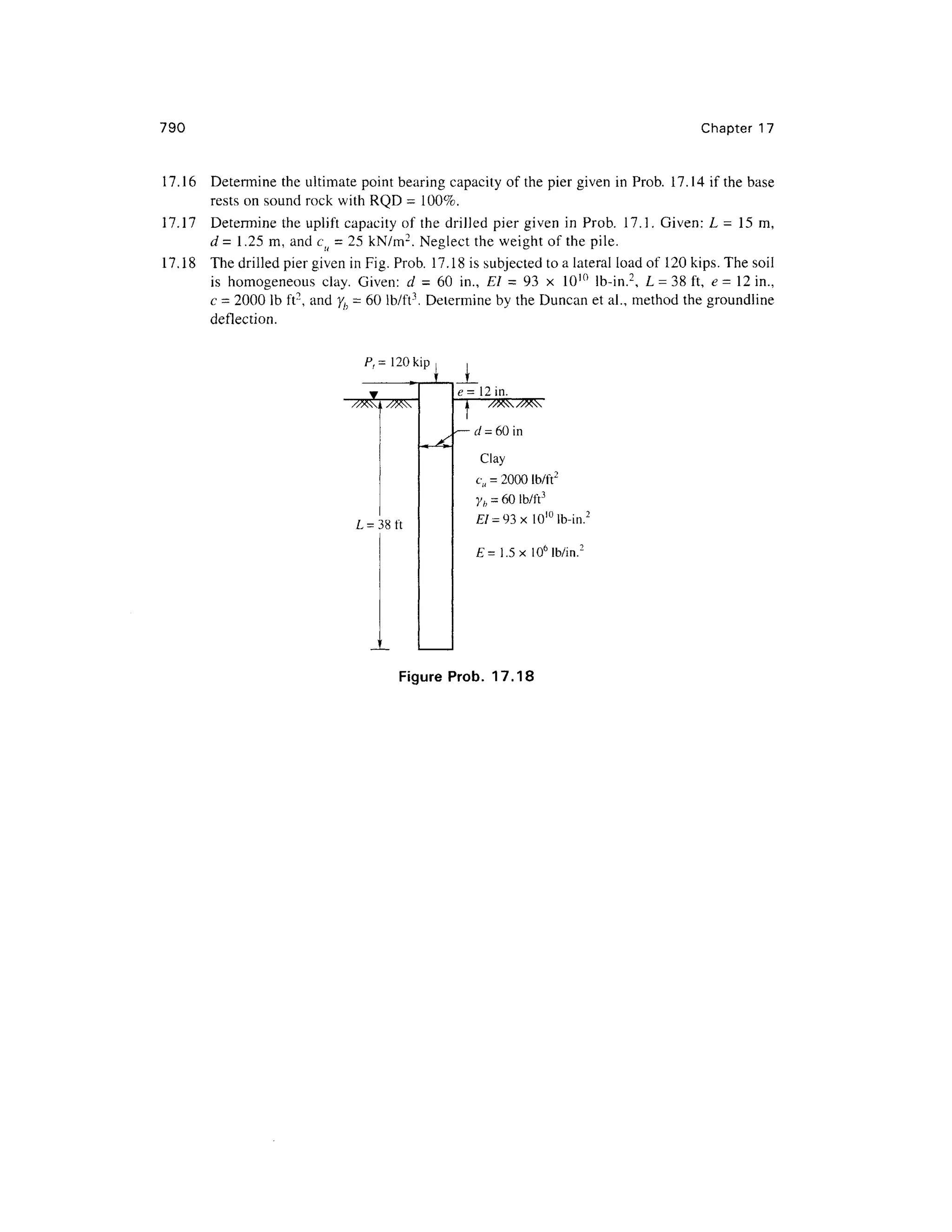
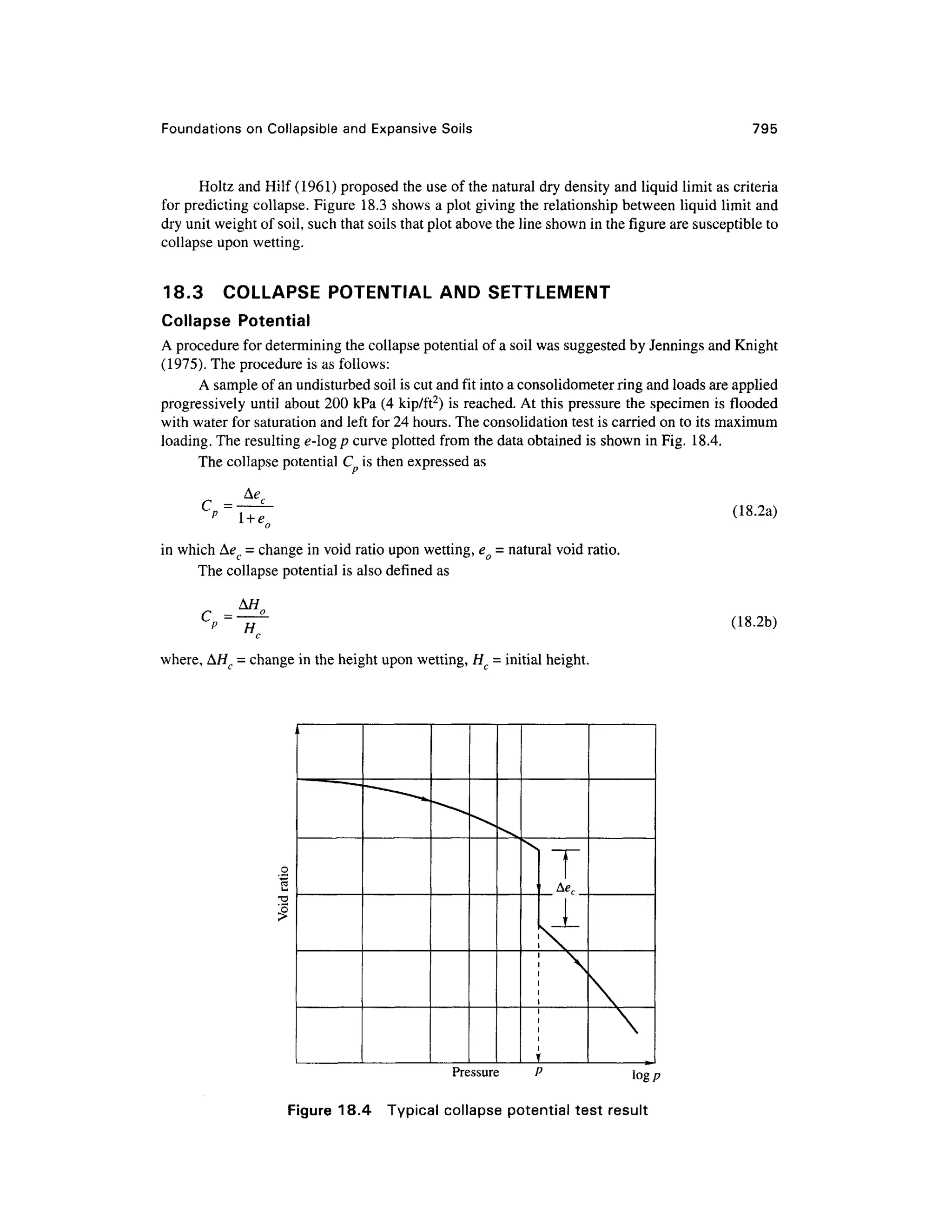
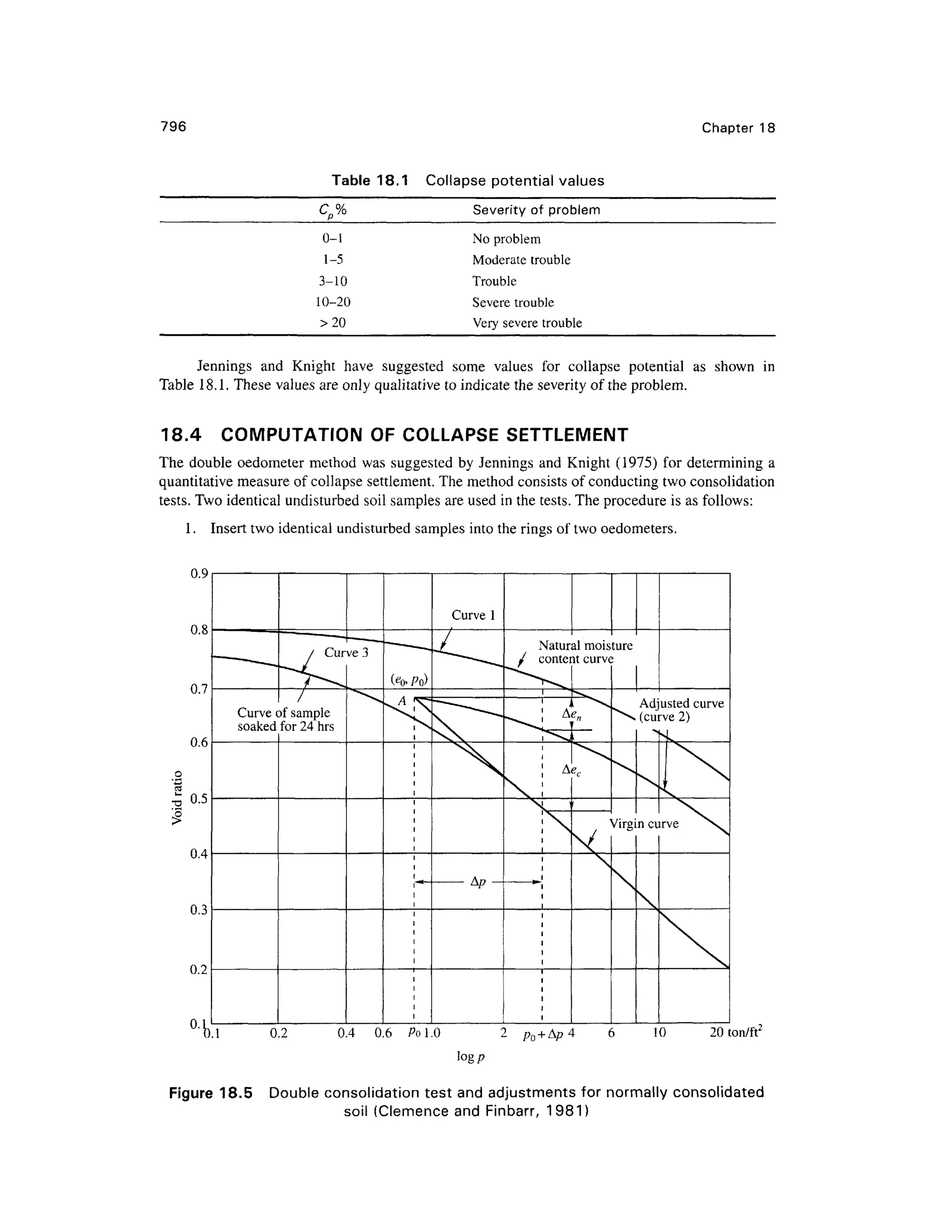
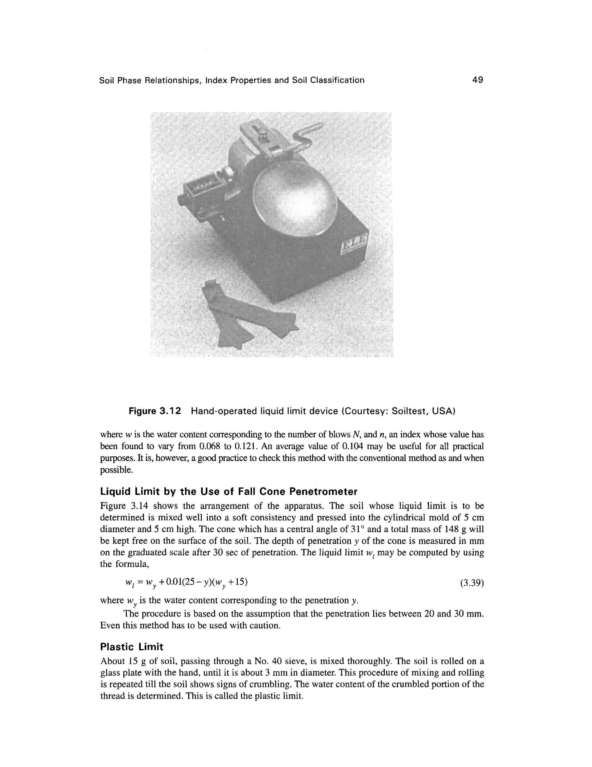
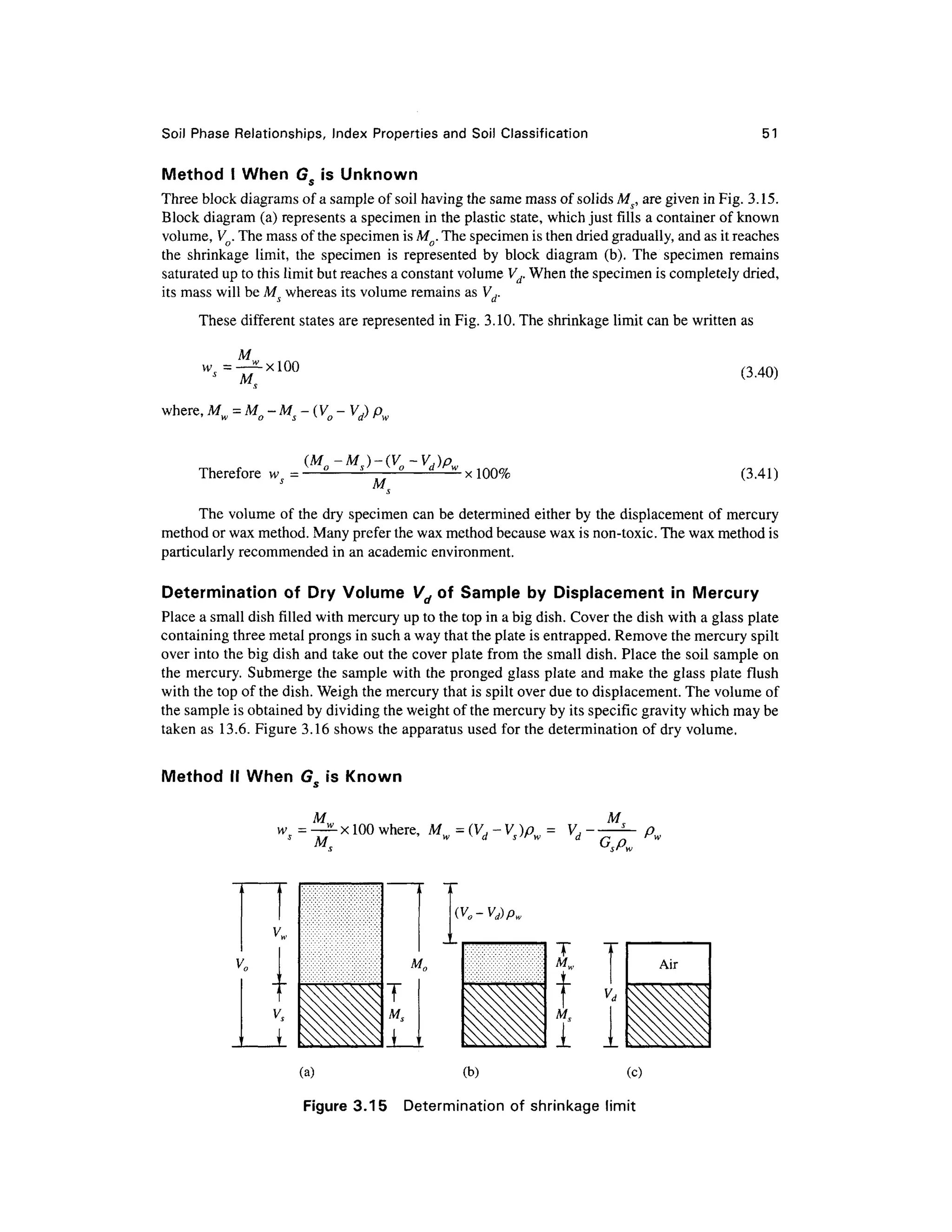
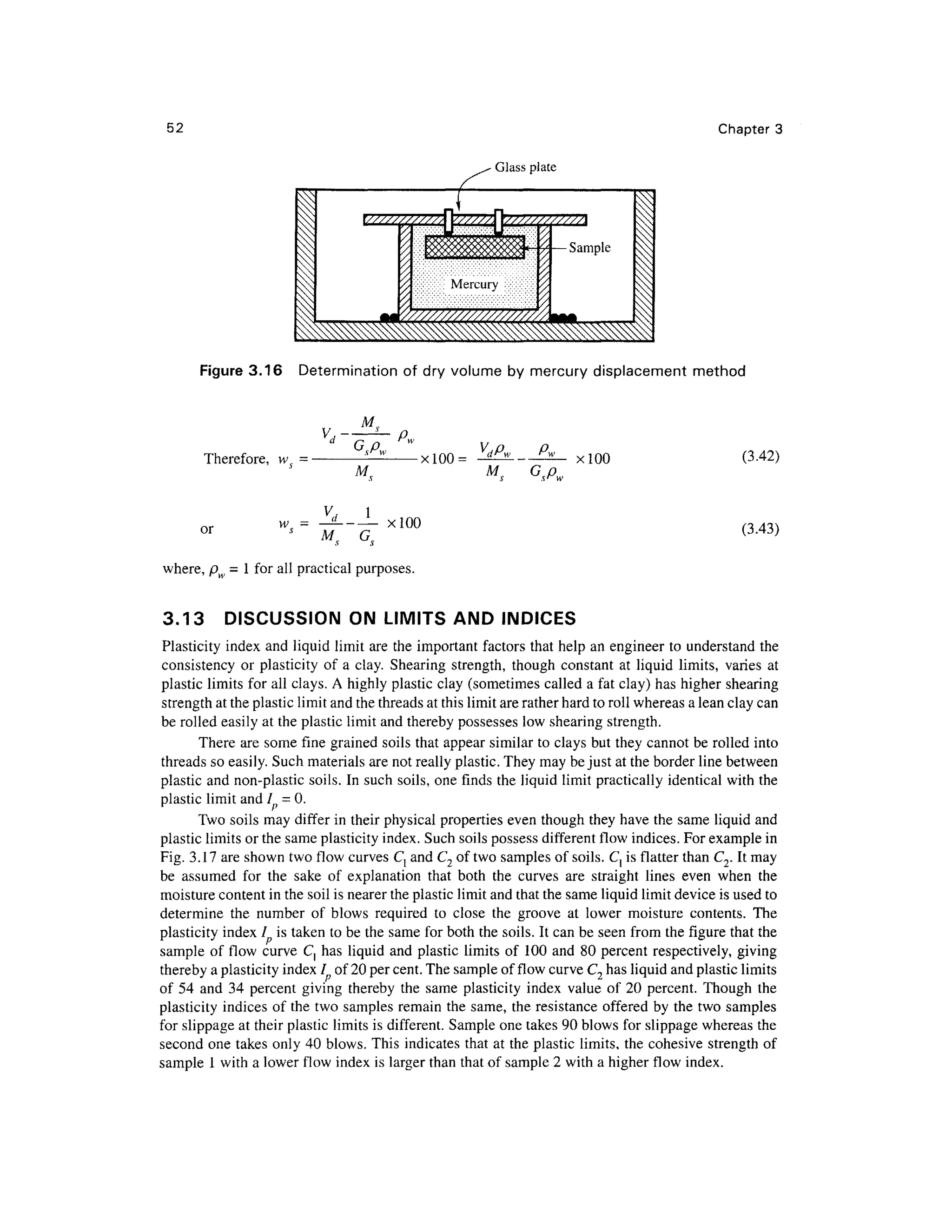
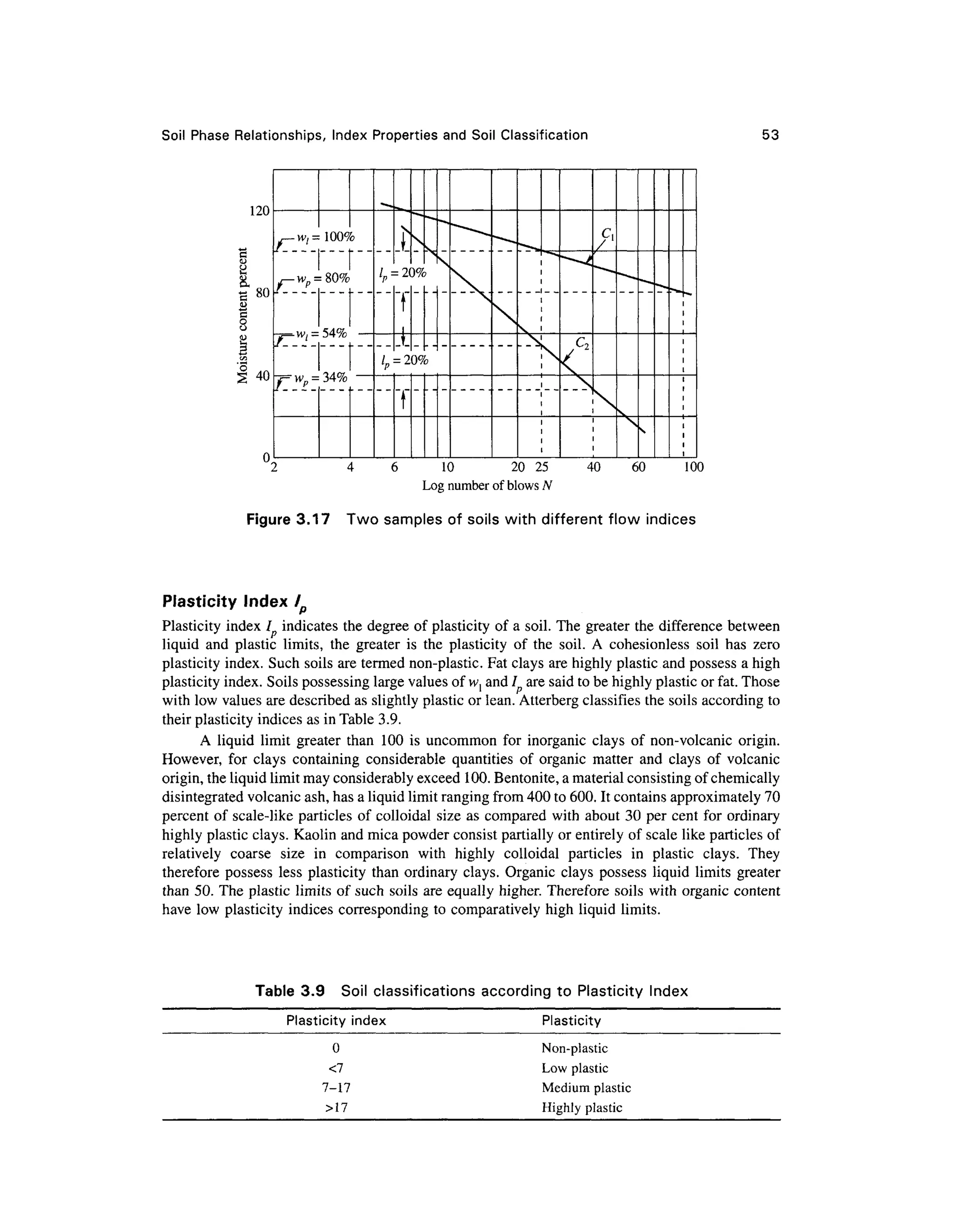
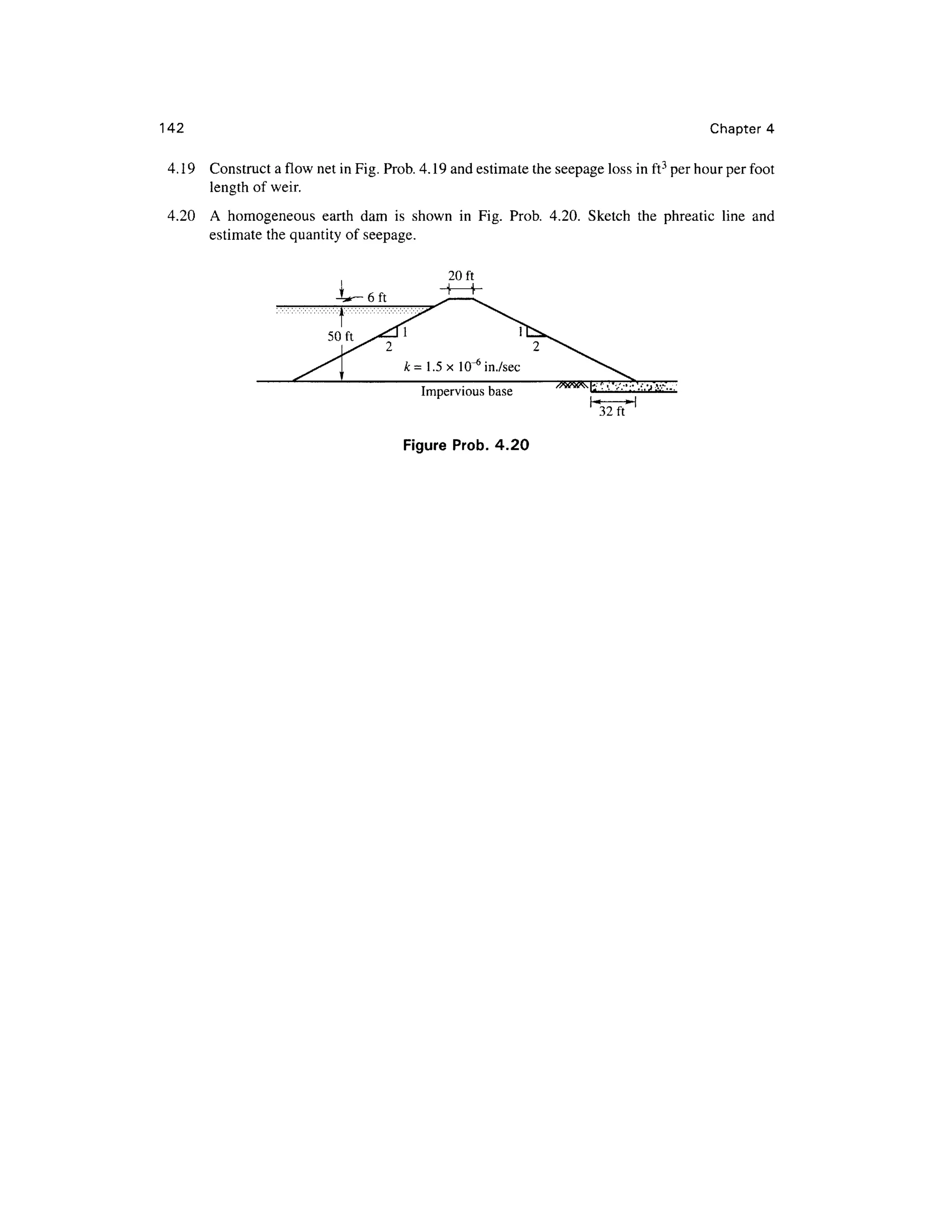
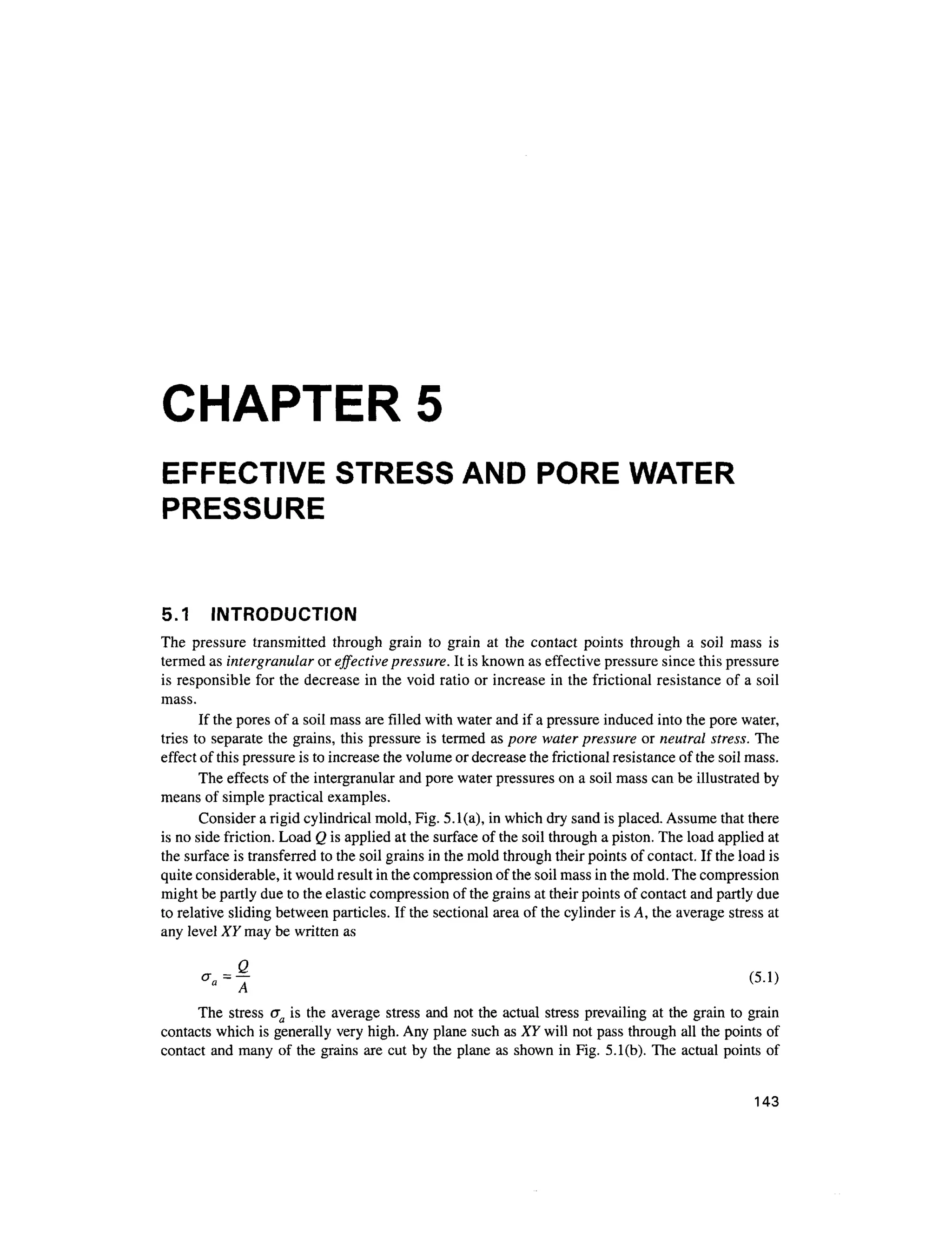
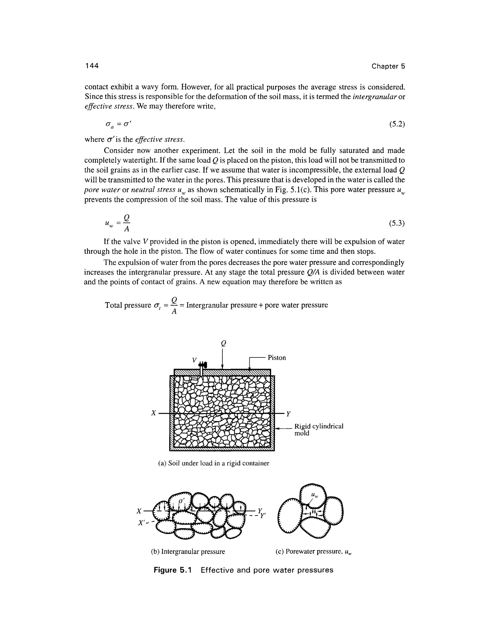
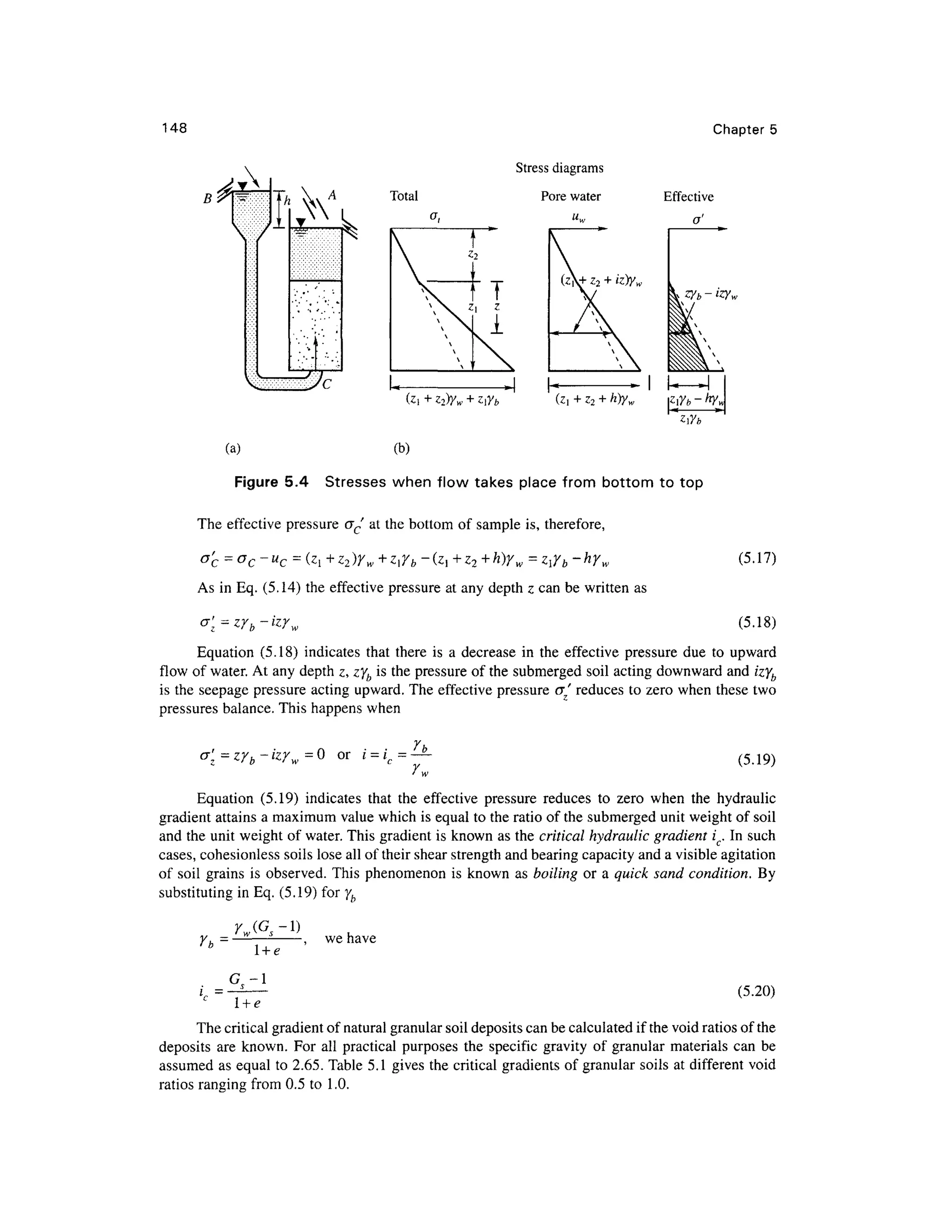
This document provides a summary and introduction to a textbook on geotechnical engineering. It discusses the comprehensive nature and logical organization of the textbook. It provides endorsements from two professors who praise the coverage, clarity, and insights provided in the textbook. They believe the textbook will be well-received and serve as a valuable reference for students, professors, and engineers. The forewords provide a high-level endorsement of the textbook's suitability and comprehensive treatment of the subject matter.

2. Dedicated to the Cause of Students

3. FOREWORD
Geotechnical Engineering: Principles and Practices of Soil Mechanics and Foundation
Engineering i s a long title befitting a major work. I am pleased t o introduce this superb volume
destined for a readership o f students, professors, an d consultants. What makes thi s text differen t
from other books on these subjects that appear each year and why am I recommending it to you? I
have been workin g and teaching in the area of geotechnical engineering for 25 years. I have read
and use d score s o f textbook s i n m y classe s an d practice . Dr . Murthy' s text i s b y fa r th e mos t
comprehensive tex t I have found. You will find that his organization of the subject matter follows
a logical progression. His example problems are numerous and, like the text, start from fundamenta l
principles an d progressivel y develo p int o mor e challengin g material . The y ar e th e bes t se t of
example problems I have seen in a textbook. Dr. Murthy has included ample homework problem s
with a rang e o f difficult y mean t t o hel p th e studen t ne w t o th e subjec t t o develo p his/he r
confidence an d t o assis t th e experience d enginee r i n his/he r revie w o f th e subjec t an d i n
professional development .
As the technical editor I have read the entire manuscript three times. I have been impressed by
the coverage, th e clarity of the presentation, and the insights into the hows and whys of soil and
foundation behavior. Often I have been astonished at Dr. Murthy's near-conversational approac h to
sharing helpfu l insights . You get th e impressio n he' s righ t ther e wit h yo u guidin g yo u along ,
anticipating your questions, and providing instruction and necessary information as the next steps
in the learning process. I believe you will enjoy this book and that it will receive a warm welcom e
wherever it is used.
I thank Dr. Murthy for his commitment to write this textbook and for sharing his professional
experience with us. I thank him for his patience in making corrections and considering suggestions.
I thank Mr. B. J. Clark, Senior Acquisitions Editor at Marcel Dekker Inc., for the opportunity to be
associated with such a good book. I likewise express my appreciation to Professor Pierre Foray of
1'Ecole National e Superieur e d'Hydrauliqu e e t d e Mecaniqu e d e Grenoble , Institu t Nationa l
Polytechnique de Grenoble, Franc e for his enthusiastic and unflagging support while I edited the
manuscript.
MarkT. Bowers, Ph.D., P. E.
Associate Professo r o f Civil Engineering
University of Cincinnati

4. FOREWORD
It give s m e grea t pleasur e t o writ e a forewor d fo r Geotechnical Engineering: Principles an d
Practices of Soil Mechanics an d Foundation Engineering. This comprehensive, pertinen t an d up-
to-date volum e i s wel l suite d fo r us e a s a textboo k fo r undergraduat e student s a s wel l a s a
reference boo k fo r consultin g geotechnica l engineers an d contractors. Thi s book is well writte n
with numerous examples on applications o f basic principles to solve practical problems.
The early history of geotechnical engineering and the pioneering work of Karl Terzaghi in
the beginning of the last century are described in Chapter 1 . Chapters 2 and 3 discuss methods of
classification of soil and rock, the chemical and the mechanical weathering of rock, and soil phase
relationships an d consistenc y limit s fo r clay s an d silts . Numerou s example s illustrat e th e
relationship between th e different parameters . Soi l permeability and seepage ar e investigated in
Chapter 4 . Th e constructio n o f flo w net s an d method s t o determin e th e permeabilit y i n th e
laboratory and in the field ar e also explained.
The concept o f effective stres s and the effect o f pore water pressure o n effective stress are
discussed in Chapter 5. Chapter 6 is concerned with stress increase in soil caused by surface load
and methods to calculate stress increase caused by spread footings, rafts, and pile groups. Several
examples are given in Chapter 6. Consolidation of soils and the evaluation of compressibility in
the laborator y b y oedomete r test s ar e investigate d in Chapte r 7 . Determinatio n o f draine d an d
undrained shea r strengt h by unconfine d compression, direc t shea r o r triaxial test s i s treated i n
Chapter 8.
The importan t subject of soi l exploratio n i s discussed i n Chapter 9 , includin g the us e of
penetration tests such as SPT and CPT in different countries. The stability of slopes is investigated
in Chapter 10 . Methods usin g plain and circular slip surfaces to evaluate stability are describe d
such a s th e method s propose d b y Bishop , Fellenius , Morgenstern , an d Spencer . Chapte r 1 1
discusses method s to determine activ e and passive earth pressures actin g on retaining and sheet
pile walls.
Bearing capacity and settlement of foundation an d the evaluation of compressibility in the
laboratory by oedometer test s are discussed in Chapters 12 , 13, and 14 . The effect o f inclination
and eccentricity of the load on bearing capacity is also examined. Chapter 1 5 describes differen t
pile types , th e concep t o f critica l depth , method s t o evaluat e th e bearin g capacit y o f pile s i n
cohesive and cohesionless soils , and pile-driving formulae. The behavior of laterally loaded pile s
is investigated in Chapter 16 for piles in sand and in clay. The behavior of drilled pier foundations
VII

5. viii Forewor d
and the effect of the installation method on bearing capacity and uplift ar e analyzed in Chapter 17.
Foundations on swelling and collapsible soils are treated i n Chapter 1 8 as are methods that can be
used t o reduc e heave . Thi s i s a n importan t subject, seldom treate d i n textbooks . Th e desig n o f
retaining wall s i s covere d i n Chapte r 19 , as wel l as th e differen t factor s tha t affec t activ e an d
passive eart h pressures. Differen t applications of geotextiles are covered in this chapter as well as
the topic of reinforced earth. Cantilever, anchored, and strutted sheet pil e walls are investigated in
Chapter 20 , a s ar e method s t o evaluat e stabilit y an d th e momen t distribution . Different soi l
improvement methods , suc h a s compactio n o f granula r soils , san d compactio n piles ,
vibroflotation, preloading , an d ston e columns , ar e describe d i n Chapte r 21 . Th e chapte r als o
discusses lim e and cemen t stabilization. Appendix A provides a list of S I units , and Appendi x B
compares methods tha t have been proposed .
This textbook b y Prof . V. N. S. Murthy is highly recommended fo r student s specializing i n
geotechnical engineerin g an d for practicing civil engineers i n the United States an d Europe . Th e
book include s recen t development s suc h a s soi l improvemen t an d stabilizatio n method s an d
applications o f geotextiles t o control settlements an d lateral earth pressure. Numerou s graph s an d
examples illustrat e th e mos t importan t concept s i n geotechnica l engineering . Thi s textboo k
should serve as a valuable reference book fo r many years to come.
BengtB.Broms, Ph.D.
Nanyang Technical University , Singapore (retired) .

6. PREFACE
This book has the following objectives:
1. T o explain the fundamentals of the subject from theor y to practice in a logical wa y
2. T o be comprehensive and meet the requirements of undergraduate students
3. T o serve as a foundation course for graduate students pursuing advanced knowledge in the
subject
There ar e 21 chapters i n this book. The first chapter traces the historical background o f the
subject and the second deal s with the formation and mineralogical composition o f soils. Chapter 3
covers th e index properties an d classification of soil. Chapters 4 and 5 explain soi l permeability,
seepage, an d th e effec t o f wate r o n stres s condition s i n soil . Stresse s develope d i n soi l du e t o
imposed surfac e loads , compressibilit y an d consolidatio n characteristics , an d shea r strengt h
characteristics o f soil ar e dealt with i n Chapters 6,7 , an d 8 respectively. The firs t eigh t chapter s
develop the necessary tool s for computing compressibility and strength characteristics o f soils.
Chapter 9 deals with methods for obtainig soil samples in the field for laboratory tests and for
determining soi l parameter s directl y by us e o f fiel d tests . Chapter s 1 0 to 2 0 dea l wit h stability
problems pertaining to earth embankments, retaining walls, and foundations. Chapter 2 1 explains
the various methods by which soil in situ can be improved. Many geotechnical engineer s hav e not
appreciated th e importanc e o f thi s subject . N o amoun t of sophisticatio n in th e developmen t of
theories will help the designers if the soil parameters used in the theory are not properly evaluated
to simulate field conditions . Professors wh o teach this subject should stress this topic.
The chapter s i n this book are arranged i n a logical wa y for the development o f the subject
matter. There is a smooth transition from one chapter to the next and the continuity of the material
is maintained. Each chapter starts with an introduction to the subject matter, develops th e theory,
and explain s it s applicatio n t o practica l problems . Sufficien t example s ar e wo r1
:ed ou t t o hel p
students understand the significance of the theories. Man y homework problem s ar e given a t the
end of each chapter .
The subjec t matte r deal t wit h i n eac h chapte r i s restricte d t o th e requirement s o f
undergraduate students. Half-baked theories an d unconfirmed test results are not developed in this
book. Chapter s ar e up-to-dat e a s pe r engineerin g standards . Th e informatio n provide d i n
Chapter 1 7 on drilled pier foundations is the latest available at the time of this writing. The design

7. Preface
of mechanically stabilized earth retaining walls is also current. A new method for predicting the
nonlinear behavior of laterally loaded vertica l and batter piles is described in Chapter 16.
The boo k i s comprehensive , rational, an d pertinen t to th e requirement s o f undergraduate
students. It serves as a foundation course for graduate students, and is useful as a reference book for
designers an d contractors in the field o f geotechnical engineering .
ACKNOWLEDGEMENTS
It is my pleasure t o thank Marcel Dekker, Inc., for accepting me as a single author for the
publication of my book. The man who was responsible for this was Mr. B.J. Clark, the Executive
Acquisition Editor . I t wa s m y pleasur e t o wor k unde r hi s guidance . Mr . Clar k i s a refine d
gentleman personified , polished , an d clea r sighted . I thank hi m cordiall y fo r the courtesie s an d
help extended to me during the course of writing the manuscript. I remain ever grateful to him.
Writing a book fo r American Universities by a nonresident o f America is not an easy task.
I neede d a n America n professo r t o edi t m y manuscrip t an d guid e m e wit h regard s t o th e
requirements of undergraduate students in America. Dr. Mark T. Bowers, Associate Professor o f
Civil Engineering, Universit y of Cincinnati, accepte d t o become m y consultant an d chief editor .
Dr. Bowers i s a man of honest y and integrity. He is dedicated t o the cause of his profession. He
worked hard for over a year in editing my book and helped me to streamline to make it acceptable
to the undergraduate student s o f American Universities. I thank Dr. Bowers for the help extended
to me.
There ar e man y i n Indi a wh o helpe d m e durin g th e cours e o f writin g thi s book . Som e
provided m e usefu l suggestion s an d other s wit h references . I acknowledg e thei r service s wit h
thanks. The members are :
Mr. S. Pranesh Managin g Directo r
Prism Books Pvt Ltd
Bangalore
Dr. K.S.Subba Rao Professo r of Civil Engineering
Indian Institute of Science Bangalor e
Dr. T.S. Nagaraj Professo r of Civil Engineering
(Emeritus), Indian Institute o f Science,
Bangalore
Professor of Civil Engineering
Dr. C. Subba Rao India n Institute of Technology
Kharagpur
Chaitanya Graphics , Bangalore , provide d th e artwor k fo r th e book . I than k M r S.K .
Vijayasimha, the designer, for the excellent job don e by him.
My so n Prakas h wa s associate d wit h th e boo k sinc e it s inception . H e carrie d o n
correspondence wit h the publishers o n m y behalf and sen t reference books a s needed. M y wif e
Sharadamani wa s mainl y responsibl e fo r keepin g m y spiri t hig h durin g th e year s I spen t i n
writing the book. I remain grateful to my son and my wife for all they did.
I sincerely thank Mr. Brian Black for his continuous effort s i n the production of this book. I
immensely thank Mr. Janardhan and Mr. Rajeshwar, compute r engineers of Aicra Info Mates Pvt
Ltd., Hyderabad, for their excellent typesetting work on this book.
V.N.S. Murthy

8. CONTENTS
Foreword Mar k T . Bowers v
Foreword Beng t B. Broms vi i
Preface i x
CHAPTER 1 INTRODUCTIO N 1
1.1 Genera l Remark s 1
1.2 A Brief Historica l Developmen t 2
1.3 Soi l Mechanic s an d Foundation Engineerin g 3
CHAPTER 2 SOI L FORMATION AND CHARACTERIZATION 5
2.1 Introductio n 5
2.2 Roc k Classificatio n 5
2.3 Formatio n o f Soil s 7
2.4 Genera l Type s o f Soil s 7
2.5 Soi l Particl e Siz e an d Shape 9
2.6 Compositio n o f Cla y Mineral s 1 1
2.7 Structur e of Clay Minerals 1 1
2.8 Cla y Particle-Wate r Relation s 1 4
2.9 Soi l Mass Structur e 1 7
XI

9. xii Content s
CHAPTER 3 SOI L PHASE RELATIONSHIPS, INDEX PROPERTIES
AND CLASSIFICATION 1 9
3.1 Soi l Phas e Relationship s 1 9
3.2 Mass-Volum e Relationships 2 0
3.3 Weight-Volum e Relationship s 2 4
3.4 Comment s o n Soi l Phas e Relationship s 2 5
3.5 Inde x Propertie s of Soils 3 1
3.6 Th e Shap e an d Siz e o f Particles 3 2
3.7 Siev e Analysi s 3 3
3.8 Th e Hydromete r Metho d o f Analysis 3 5
3.9 Grai n Siz e Distributio n Curves 4 3
3.10 Relativ e Densit y o f Cohesionless Soil s 4 4
3.11 Consistenc y o f Cla y Soi l 4 5
3.12 Determinatio n of Atterberg Limit s 4 7
3.13 Discussio n o n Limits an d Indices 5 2
3.14 Plasticit y Char t 5 9
3.15 Genera l Consideration s fo r Classification o f Soil s 6 7
3.16 Fiel d Identificatio n of Soil s 6 8
3.17 Classificatio n o f Soil s 6 9
3.18 Textura l Soi l Classificatio n 6 9
3.19 AASHT O Soi l Classificatio n System 7 0
3.20 Unifie d Soi l Classificatio n Syste m (USCS ) 7 3
3.21 Comment s o n th e System s o f Soi l Classificatio n 7 6
3.22 Problem s 8 0
CHAPTER 4 SOI L PERMEABILITY AND SEEPAGE 8 7
4.1 Soi l Permeabilit y 8 7
4.2 Darcy' s La w 8 9
4.3 Discharg e an d Seepag e Velocitie s 9 0
4.4 Method s o f Determinatio n of Hydrauli c Conductivity of Soil s 9 1
4.5 Constan t Hea d Permeabilit y Tes t 92
4.6 Fallin g Hea d Permeabilit y Tes t 9 3
4.7 Direc t Determinatio n of k o f Soil s i n Plac e b y Pumpin g Test 9 7
4.8 Borehol e Permeabilit y Test s 10 1
4.9 Approximat e Value s o f th e Hydrauli c Conductivity of Soil s 10 2
4.10 Hydrauli c Conductivit y in Stratifie d Layer s o f Soil s 10 2
4.11 Empirica l Correlation s fo r Hydrauli c Conductivity 10 3
4.12 Hydrauli c Conductivity of Rock s b y Packe r Metho d 11 2
4.13 Seepag e 11 4
4.14 Laplac e Equatio n 11 4

10. Contents xii i
4.15 Flo w Ne t Constructio n 11 6
4.16 Determinatio n o f Quantit y of Seepag e 12 0
4.17 Determinatio n o f Seepag e Pressur e 12 2
4.18 Determinatio n o f Uplif t Pressure s 12 3
4.19 Seepag e Flo w Throug h Homogeneou s Eart h Dam s 12 6
4.20 Flo w Ne t Consistin g o f Conjugat e Confocal Parabola s 12 7
4.21 Pipin g Failur e 13 1
4.22 Problem s 13 8
CHAPTER 5 EFFECTIV E STRESS AND PORE WATER PRESSURE 14 3
5.1 Introductio n 14 3
5.2 Stresse s whe n No Flo w Take s Plac e Through th e
Saturated Soi l Mas s 14 5
5.3 Stresse s Whe n Flo w Take s Plac e Through the Soi l
from To p to Botto m 14 6
5.4 Stresse s Whe n Flo w Take s Plac e Throug h th e Soi l
from Botto m t o Top 14 7
5.5 Effectiv e Pressur e Du e to Capillary Wate r Ris e i n Soi l 14 9
5.6 Problem s 17 0
CHAPTER 6 STRES S DISTRIBUTIO N IN SOILS
DUE TO SURFACE LOADS 17 3
6.1 Introductio n 17 3
6.2 Boussinesq' s Formul a fo r Poin t Load s 17 4
6.3 Westergaard' s Formul a fo r Point Load s 17 5
6.4 Lin e Load s 17 8
6.5 Stri p Load s 17 9
6.6 Stresse s Beneat h th e Corne r o f a Rectangular Foundation 18 1
6.7 Stresse s Unde r Uniformly Loade d Circula r Footin g 18 6
6.8 Vertica l Stress Beneat h Loade d Area s o f Irregula r Shap e 18 8
6.9 Embankmen t Loading s 19 1
6.10 Approximat e Method s fo r Computin g c r 19 7
6.11 Pressur e Isobar s 19 8
6.12 Problem s 20 3
CHAPTER 7 COMPRESSIBILIT Y AN D CONSOLIDATION 20 7
7.1 Introductio n 20 7
7.2 Consolidatio n 20 8
7.3 Consolidomete r 21 2

11. xiv Content s
7.4 Th e Standar d One-Dimensiona l Consolidatio n Tes t 21 3
7.5 Pressure-Voi d Rati o Curve s 21 4
7.6 Determinatio n of Preconsolidatio n Pressur e 21 8
7.7 e-logp Fiel d Curves for Normally Consolidate d and
Overconsolidated Clay s of Low to Medium Sensitivit y 21 9
7.8 Computatio n of Consolidatio n Settlemen t 21 9
7.9 Settlemen t Du e t o Secondar y Compressio n 22 4
7.10 Rat e o f One-dimensiona l Consolidation Theory o f Terzaghi 23 3
7.11 Determinatio n of th e Coefficien t o f Consolidatio n 24 0
7.12 Rat e o f Settlemen t Du e to Consolidatio n 24 2
7.13 Two - and Three-dimensional Consolidatio n Problems 24 3
7.14 Problem s 24 7
CHAPTERS SHEA R STRENGTH O F SOIL 25 3
8.1 Introductio n 25 3
8.2 Basi c Concep t o f Shearin g Resistanc e an d Shearin g Strengt h 25 3
8.3 Th e Coulom b Equatio n 25 4
8.4 Method s o f Determinin g Shea r Strengt h Parameters 25 5
8.5 Shea r Tes t Apparatu s 25 6
8.6 Stres s Conditio n at a Point in a Soil Mas s 26 0
8.7 Stres s Condition s in Soi l Durin g Triaxial Compressio n Tes t 26 2
8.8 Relationshi p Between th e Principal Stresse s an d Cohesion c 26 3
8.9 Moh r Circl e o f Stress 26 4
8.10 Moh r Circl e of Stres s When a Prismatic Elemen t i s Subjecte d to
Normal an d Shear Stresse s 26 5
8.11 Moh r Circl e o f Stres s fo r a Cylindrical Specime n
Compression Tes t 26 6
8.12 Mohr-Coulom b Failur e Theor y 26 8
8.13 Moh r Diagra m fo r Triaxial Compressio n Tes t a t Failure 26 9
8.14 Moh r Diagra m fo r a Direct Shea r Test a t Failure 27 0
8.15 Effectiv e Stresse s 27 4
8.16 Shea r Strengt h Equatio n i n Terms o f Effective Principa l Stresse s 27 5
8.17 Stress-Controlle d an d Strain-Controlled Test s 27 6
8.18 Type s o f Laborator y Tests 27 6
8.19 Shearin g Strengt h Tests o n San d 27 8
8.20 Unconsolidated-Undraine d Test 28 4
8.21 Unconfine d Compression Test s 28 6
8.22 Consolidated-Undraine d Tes t o n Saturate d Cla y 29 4
8.23 Consolidated-Draine d Shear Strengt h Tes t 29 6
8.24 Por e Pressur e Parameter s Unde r Undraine d Loadin g 29 8
8.25 Van e Shea r Tests 30 0

12. Contents x v
8.26 Othe r Method s fo r Determinin g Undraine d Shea r Strengt h
of Cohesiv e Soil s 30 2
8.27 Th e Relationshi p Between Undraine d Shear Strengt h an d
Effective Overburde n Pressure 30 4
8.28 Genera l Comment s 31 0
8.29 Question s and Problems 31 1
CHAPTERS SOI L EXPLORATIO
N 31 7
9.1 Introductio n 31 7
9.2 Borin g of Hole s 31 8
9.3 Samplin g in Soil 32 2
9.4 Roc k Cor e Samplin g 32 5
9.5 Standar d Penetration Test 32 7
9.6 SP T Values Related t o Relative Density of Cohesionless Soil s 33 0
9.7 SP T Values Related t o Consistency of Clay Soi l 33 0
9.8 Stati c Con e Penetratio n Test (CPT ) 33 2
9.9 Pressuremete r 34 3
9.10 Th e Flat Dilatomete r Test 34 9
9.11 Fiel d Vane Shear Test (VST) 35 1
9.12 Fiel d Plat e Load Test (PUT ) 3 51
9.13 Geophysica l Exploratio n 35 2
9.14 Plannin g of Soi l Exploratio n 35 8
9.15 Executio n of Soi l Exploratio n Progra m 35 9
9.16 Repor t 36 1
9.17 Problem s 36 2
CHAPTER 1 0 STABILIT Y O F SLOPES 36 5
10.1 Introductio n 36 5
10.2 Genera l Consideration s an d Assumptions in th e Analysis 36 7
10.3 Facto r o f Safet y 36 8
10.4 Stabilit y Analysi s of Infinit e Slope s i n Sand 37 1
10.5 Stabilit y Analysis of Infinit e Slope s i n Clay 37 2
10.6 Method s o f Stabilit y Analysis of Slopes o f Finite Heigh t 37 6
10.7 Plan e Surfac e of Failur e 37 6
10.8 Circula r Surface s of Failure 37 8
10.9 Failur e Unde r Undrained Condition s((f> u = 0 ) 38 0
10.10 Friction-Circl e Metho d 38 2
10.11 Taylor' s Stabilit y Number 38 9
10.12 Tensio n Crack s 39 3
10.13 Stabilit y Analysis by Method o f Slice s fo r Stead y Seepag e 39 3

13. xvi Content s
10.14 Bishop' s Simplifie d Metho d o f Slice s 40 0
10.15 Bisho p an d Morgenster n Metho d fo r Slop e Analysi s 40 3
10.16 Morgenster n Metho d o f Analysis for Rapi d Drawdow n Conditio n 40 5
10.17 Spence r Metho d o f Analysis 40 8
10.18 Problem s 41 1
CHAPTER 1 1 LATERA L EARTH PRESSURE 41 9
11.1 Introductio n 41 9
11.2 Latera l Eart h Pressur e Theor y 42 0
11.3 Latera l Eart h Pressur e fo r a t Rest Conditio n 42 1
11.4 Rankine' s State s o f Plasti c Equilibriu m for Cohesionles s Soil s 42 5
11.5 Rankine' s Eart h Pressur e Agains t Smoot h Vertica l Wall with
Cohesionless Backfil l 42 8
11.6 Rankine' s Activ e Earth Pressur e wit h Cohesiv e Backfil l 44 0
11.7 Rankine' s Passiv e Eart h Pressur e wit h Cohesiv e Backfil l 44 9
11.8 Coulomb' s Eart h Pressur e Theor y fo r San d fo r Active Stat e 45 2
11.9 Coulomb' s Eart h Pressur e Theor y fo r San d fo r Passiv e Stat e 45 5
11.10 Activ e Pressur e by Culmann' s Metho d fo r Cohesionles s Soil s 45 6
11.11 Latera l Pressure s b y Theor y o f Elasticit y fo r Surcharg e Load s
on th e Surfac e of Backfil l 45 8
11.12 Curve d Surface s o f Failur e fo r Computin g Passiv e Eart h Pressur e 46 2
11.13 Coefficient s of Passiv e Eart h Pressur e Table s an d Graph s 46 4
11.14 Latera l Eart h Pressur e o n Retainin g Walls Durin g Earthquake s 46 7
11.15 Problem s 47 6
CHAPTER 1 2 SHALLO W FOUNDATION I:
ULTIMATE BEARING CAPACITY 48 1
12.1 Introductio n 48 1
12.2 Th e Ultimat e Bearing Capacit y o f Soi l 48 3
12.3 Som e o f th e Terms Define d 48 3
12.4 Type s o f Failur e in Soi l 48 5
12.5 A n Overvie w o f Bearin g Capacit y Theorie s 48 7
12.6 Terzaghi' s Bearin g Capacit y Theor y 48 8
12.7 Skempton' s Bearin g Capacit y Facto r N C 49 3
12.8 Effec t o f Water Tabl e o n Bearin g Capacit y 49 4
12.9 Th e Genera l Bearin g Capacit y Equatio n 50 3
12.10 Effec t o f Soi l Compressibilit y o n Bearin g Capacit y o f Soi l 50 9
12.11 Bearin g Capacit y o f Foundation s Subjecte d t o Eccentri c Load s 51 5
12.12 Ultimat e Bearin g Capacit y o f Footing s Base d o n SP T Value s (N) 51 8
12.13 Th e CP T Metho d o f Determinin g Ultimat e Bearin g Capacit y 51 8

14. Contents xvi i
12.14 Ultimat e Bearin g Capacit y o f Footings Restin g o n Stratifie d
Deposits o f Soi l 52 1
12.15 Bearin g Capacit y o f Foundations o n Top of a Slop e 52 9
12.16 Foundation s o n Roc k 53 2
12.17 Cas e Histor y of Failure o f the Transcona Grai n Elevato r 53 3
12.18 Problem s 53 6
CHAPTER 13 SHALLO W FOUNDATION II:
SAFE BEARING PRESSURE AND SETTLEMENT CALCULATION 54 5
13.1 Introductio n 54 5
13.2 Fiel d Plat e Loa d Test s 54 8
13.3 Effec t o f Siz e o f Footings o n Settlemen t 55 4
13.4 Desig n Chart s fro m SP T Values for Footings o n San d 55 5
13.5 Empirica l Equation s Base d o n SP T Values for Footing s o n
Cohesionless Soil s 55 8
13.6 Saf e Bearing Pressur e fro m Empirica l Equation s Based o n
CPT Values for Footings o n Cohesionless Soi l 55 9
13.7 Foundatio n Settlemen t 56 1
13.8 Evaluatio n of Modulu s of Elasticit y 56 2
13.9 Method s o f Computing Settlements 56 4
13.10 Elasti c Settlemen t Beneat h the Corner o f a Uniformly Loade d
Flexible Are a Based o n the Theory o f Elasticity 56 5
13.11 Janbu , Bjerrum an d Kjaernsli' s Metho d o f Determinin g
Elastic Settlemen t Unde r Undrained Conditions 56 8
13.12 Schmertmann' s Metho d o f Calculatin g Settlemen t i n Granular
Soils b y Using CPT Values 56 9
13.13 Estimatio n o f Consolidatio n Settlemen t b y Usin g Oedometer
Test Dat a 57 5
13.14 Skempton-Bjerru m Metho d o f Calculatin g Consolidatio n
Settlement (1957 ) 57 6
13.15 Problem s 58 0
CHAPTER 14 SHALLO W FOUNDATION III:
COMBINED FOOTINGS AND MAT FOUNDATIONS 58 5
14.1 Introductio n 58 5
14.2 Saf e Bearin g Pressure s fo r Ma t Foundation s on San d an d Clay 58 7
14.3 Eccentri c Loadin g 58 8
14.4 Th e Coefficien t of Subgrad e Reactio n 58 8
14.5 Proportionin g o f Cantileve r Footin g 59 1

15. xviii Content s
14.6 Desig n o f Combine d Footing s b y Rigi d Metho d (Conventiona l
Method) 59 2
14.7 Desig n o f Ma t Foundatio n b y Rigi d Metho d 59 3
14.8 Desig n o f Combined Footing s b y Elasti c Lin e Metho d 59 4
14.9 Desig n o f Mat Foundation s by Elasti c Plat e Metho d 59 5
14.10 Floatin g Foundatio n 59 5
14.11 Problem s 60 3
CHAPTER 15 DEE P FOUNDATION I :
PILE FOUNDATION 60 5
15.1 Introductio n 60 5
15.2 Classificatio n of Piles 605
15.3 Type s o f Piles Accordin g to the Metho d o f Installation 60 6
15.4 Use s o f Piles 60 8
15.5 Selectio n o f Pile 60 9
15.6 Installatio n of Piles 61 0
PART A-VERTICAL LOAD BEARING CAPACITY OF ASINGLE VERTICAL PILE 61 3
15.7 Genera l Consideration s 61 3
15.8 Method s o f Determinin g Ultimat e Load Bearin g Capacit y o f a
Single Vertical Pile 61 7
15.9 Genera l Theor y fo r Ultimat e Bearing Capacit y 61 8
15.10 Ultimat e Bearin g Capacit y i n Cohesionless Soil s 62 0
15.11 Critica l Dept h 62 1
15.12 Tomlinson' s Solutio n fo r Qbin Sand 62 2
15.13 Meyerhof' s Metho d o f Determining Q bfor Pile s i n San d 62 4
15.14 Vesic' s Metho d o f Determinin g Q b 62 5
15.15 Janbu' s Metho d o f Determining Qb 62 8
15.16 Coyl e an d Castello's Metho d o f Estimating Qbin Sand 62 8
15.17 Th e Ultimat e Skin Resistanc e of a Single Pile i n Cohesionless Soi l 62 9
15.18 Ski n Resistanc e Q fby Coyl e an d Castell o Metho d (1981 ) 63 1
15.19 Stati c Bearin g Capacity of Piles i n Clay Soi l 63 1
15.20 Bearin g Capacit y of Piles i n Granular Soil s Base d o n SP T Value 63 5
15.21 Bearin g Capacit y o f Piles Base d o n Stati c Con e Penetratio n
Tests (CPT ) 65 2
15.22 Bearin g Capacit y o f a Singl e Pile b y Loa d Tes t 66 3
15.23 Pil e Bearing Capacity fro m Dynamic Pile Driving Formulas 66 6
15.24 Bearin g Capacit y o f Piles Founde d o n a Rock y Be d 67 0
15.25 Uplif t Resistanc e o f Pile s 67 1

16. Contents xi x
PART B-PILE GROUP 67 4
15.26 Numbe r an d Spacin g o f Piles i n a Group 67 4
15.27 Pil e Grou p Efficienc y 67 6
15.28 Vertica l Bearin g Capacity o f Pile Group s Embedded i n
Sands an d Gravels 67 8
15.29 Settlemen t o f Piles an d Pile Group s i n Sands an d Gravels 68 1
15.30 Settlemen t of Pile Group s in Cohesive Soil s 68 9
15.31 Allowabl e Loads o n Groups o f Piles 69 0
15.32 Negativ e Frictio n 69 2
15.33 Uplif t Capacit y o f a Pile Grou p 69 4
15.34 Problem s 69 6
CHAPTER 16 DEE P FOUNDATION II :
BEHAVIOR OF LATERALLY LOADED VERTICAL AND
BATTER PILES 69 9
16.1 Introductio n 69 9
16.2 Winkler' s Hypothesi s 70 0
16.3 Th e Differential Equatio n 70 1
16.4 Non-dimensiona l Solution s fo r Vertical Piles Subjecte d t o
Lateral Load s 70 4
16.5 p- y Curve s for the Solutio n o f Laterally Loade d Pile s 70 6
16.6 Broms ' Solution s fo r Laterally Loade d Pile s 70 9
16.7 A Direct Metho d fo r Solvin g th e Non-linear Behavio r of
Laterally Loade d Flexibl e Pil e Problem s 71 6
16.8 Cas e Studies fo r Laterally Loade d Vertical Pile s in San d 72 2
16.9 Cas e Studie s for Laterally Loade d Vertica l Piles in Clay 72 5
16.10 Behavio r o f Laterally Loade d Batte r Pile s i n Sand 73 1
16.11 Problem s 73 9
CHAPTER 17 DEE P FOUNDATION III :
DRILLED PIER FOUNDATIONS 74 1
17.1 Introductio n 74 1
17.2 Type s o f Drilled Pier s 7 4
1
17.3 Advantage s and Disadvantage s o f Drilled Pie r Foundation s 74 3
17.4 Method s o f Constructio n 74 3
17.5 Desig n Consideration s 75 1
17.6 Loa d Transfe r Mechanis m 75 2
17.7 Vertica l Bearing Capacit y o f Drilled Pier s 75 4
17.8 Th e Genera l Bearin g Capacit y Equatio n fo r the Bas e Resistanc e
= 75 5
"

17. xx Content s
17.9 Bearin g Capacit y Equation s fo r the Bas e i n Cohesiv e Soi l 75 6
17.10 Bearin g Capacit y Equatio n fo r the Bas e i n Granula r Soi l 75 6
17.11 Bearin g Capacit y Equation s fo r th e Base i n Cohesive IG M o r Rock 75 9
17.12 Th e Ultimat e Ski n Resistanc e o f Cohesiv e and
Intermediate Material s 76 0
17.13 Ultimat e Ski n Resistanc e i n Cohesionles s Soi l an d Gravell y Sand s 76 3
17.14 Ultimat e Side an d Tota l Resistanc e i n Roc k 76 4
17.15 Estimatio n o f Settlement s of Drille d Pier s a t Working Load s 76 5
17.16 Uplif t Capacit y o f Drille d Pier s 77 7
17.17 Latera l Bearin g Capacit y o f Drille d Pier s 77 9
17.18 Cas e Stud y of a Drille d Pier Subjecte d t o Lateral Load s 78 7
17.19 Problem s 78 7
CHAPTER 18 FOUNDATION S ON COLLAPSIBLE AND
EXPANSIVE SOIL S 79 1
18.1 Genera l Consideration s 79 1
PART A-COLLAPSIBLE SOILS 79 3
18.2 Genera l Observation s 79 3
18.3 Collaps e Potentia l an d Settlemen t 79 5
18.4 Computatio n o f Collaps e Settlemen t 79 6
18.5 Foundatio n Desig n 79 9
18.6 Treatmen t Method s fo r Collapsibl e Soil s 80 0
PART B-EXPANSIVE SOILS 80 0
18.7 Distributio n of Expansiv e Soil s 80 0
18.8 Genera l Characteristic s of Swellin g Soil s 80 1
18.9 Cla y Mineralog y an d Mechanis m o f Swellin g 80 3
18.10 Definitio n o f Som e Parameter s 80 4
18.11 Evaluatio n o f th e Swellin g Potentia l o f Expansiv e Soil s b y Singl e
Index Metho d 80 4
18.12 Classificatio n o f Swellin g Soil s b y Indirec t Measuremen t 80 6
18.13 Swellin g Pressure b y Direc t Measuremen t 81 2
18.14 Effec t o f Initia l Moistur e Conten t an d Initia l Dry Densit y o n
Swelling Pressur e 81 3
18.15 Estimatin g the Magnitud e of Swellin g 81 4
18.16 Desig n o f Foundation s i n Swellin g Soil s 81 7
18.17 Drille d Pie r Foundation s 81 7
18.18 Eliminatio n of Swellin g 82 7
18.19 Problem s 82 8

18. Contents xx i
CHAPTER 19 CONCRET E AND MECHANICALLY STABILIZED
EARTH RETAINING WALLS 83 3
PART A-CONCRETE RETAINING WALL S 83 3
19.1 Introductio n 83 3
19.2 Condition s Unde r Which Rankin e an d Coulomb Formula s Ar e
Applicable t o Retainin g Walls Unde r th e Active Stat e 83 3
19.3 Proportionin g o f Retainin g Walls 83 5
19.4 Eart h Pressur e Chart s fo r Retainin g Walls 83 6
19.5 Stabilit y of Retainin g Walls 83 9
PART B-MECHANICALLY STABILIZED EART H RETAINING WALL S 84 9
19.6 Genera l Consideration s 84 9
19.7 Backfil l an d Reinforcing Material s 85 1
19.8 Constructio n Detail s 85 5
19.9 Desig n Consideration s fo r a Mechanically Stabilize d Eart h Wal l 85 7
19.10 Desig n Metho d 85 9
19.11 Externa l Stabilit y 86 3
19.12 Example s o f Measured Latera l Eart h Pressure s 87 5
19.13 Problem s 87 7
CHAPTER 20 SHEE T PILE WALLS AND BRACED CUTS 88 1
20.1 Introductio n 88 1
20.2 Shee t Pil e Structure s 88 3
20.3 Fre e Cantileve r Shee t Pil e Walls 88 3
20.4 Dept h o f Embedmen t o f Cantileve r Walls i n Sand y Soil s 88 5
20.5 Dept h o f Embedmen t o f Cantileve r Walls in Cohesiv e Soil s 89 6
20.6 Anchore d Bulkhead : Free-Eart h Suppor t Method—Dept h o f
Embedment o f Anchored Shee t Pile s i n Granula r Soil s 90 8
20.7 Desig n Chart s fo r Anchored Bulkhead s in San d 91 3
20.8 Momen t Reductio n fo r Anchored Shee t Pil e Walls 91 6
20.9 Anchorag e o f Bulkhead s 92 5
20.10 Brace d Cut s 93 1
20.11 Latera l Eart h Pressur e Distributio n on Braced-Cuts 93 5
20.12 Stabilit y o f Brace d Cut s i n Saturate d Clay 93 8
20.13 Bjerru m an d Eid e Metho d o f Analysis 94 0
20.14 Pipin g Failure s i n Sand Cut s 94 5
20.15 Problem s 94 5

19. X X I I Contents
CHAPTER 21 SOI L IMPROVEMENT
21.1 Introductio n
21.2 Mechanica l Compaction
21.3 Laborator y Test s o n Compaction
21.4 Effec t o f Compactio n o n Engineerin g Behavio r
21.5 Fiel d Compactio n an d Contro l
21.6 Compactio n fo r Deepe r Layer s o f Soi l
21.7 Preloadin g
21.8 San d Compactio n Pile s an d Ston e Column s
21.9 Soi l Stabilizatio n by th e Us e o f Admixtures
21.10 Soi l Stabilizatio n by Injectio n of Suitabl e Grouts
21.11 Problem s
951
951
952
953
959
962
973
974
980
981
983
983
APPENDIX A S I UNITS IN GEOTECHNICAL ENGINEERING 987
APPENDIX B SLOP E STABILITY CHART S AND TABLES 993
REFERENCES 1007
INDEX 1025

20. CHAPTER 1
INTRODUCTION
1.1 GENERA L REMARK S
Karl Terzaghi writing in 1951 (Bjerrum, et. al., 1960), on 'The Influence of Modern Soil Studies on
the Design and Construction of Foundations' commente d on foundations as follows:
Foundations can appropriately be described as a necessary evil. If a building is to be
constructed on an outcrop of sound rock, no foundationis required. Hence, in contrast to the
building itself which satisfies specific needs, appeals to the aesthetic sense, and fills its
matters with pride, the foundationsmerely serve as a remedy for the deficiencies of whatever
whimsical nature has provided for the support of the structure at the site which has been
selected. On account of the fact that there is no glory attached to the foundations, and that
the sources of success or failures are hidden deep in the ground, building foundations have
always been treated as step children; and their acts of revenge forthe lack of attention can be
very embarrassing.
The comment s mad e by Terzaghi ar e very significan t an d shoul d be take n note of by all
practicing Architects and Engineers. Architects or Engineers who do not wish to make use of the
growing knowledge of foundation design are not rendering true service to their profession. Sinc e
substructures are as important as superstructures, persons who are well qualified in the design of
substructures shoul d alway s b e consulted an d the old proverb that a 'stitc h in time saves nine'
should always be kept in mind.
The design of foundations is a branch of Civil Engineering. Experience has shown that most
of these branches have passed in succession through two stages, the empirical an d the scientific,
before they reached th e present one which may be called the stage of maturity.
The stage of scientific reasoning in the design of foundations started with the publication of
the book Erdbaumechanik (means Soil Mechanics) by Karl Terzaghi in 1925. This book represents
the first attempt to treat Soil Mechanics on the basis of the physical properties o f soils. Terzaghi's

21. Chapter 1
contribution for the development of Soil Mechanics and Foundation Engineering is so vast that he
may truly be called the Father o f Soil Mechanics, Hi s activity extended over a period of about 50
years starting from th e year 1913. He was born on October 2, 188 3 in Prague and died on October
25, 196 3 i n Winchester, Massachusetts, USA. His amazing career is well documented in the book
'From Theory t o Practice in Soil Mechanics' (Bjerrum , L., et. al., 1960) .
Many investigator s in the field of Soil Mechanics were inspired by Terzaghi. Som e o f th e
notable personalitie s wh o followe d hi s footstep s ar e Ralp h B . Peck , Arthu r Casagrande ,
A. W. Skempton, etc. Because of the unceasing efforts of these and other innumerable investigators,
Soil Mechanics and Foundation Engineering ha s come to stay as a very important par t of the Civil
Engineering profession.
The transitio n of foundation engineering fro m th e empirica l stag e t o tha t of th e scientific
stage started almos t a t the commencement o f the 20th century. The design o f foundations during
the empirical stage was based mostly on intuition and experience. There use d to be many failures
since the procedure of design was only by trial and error.
However, in the present scientific age, the design of foundations based on scientific analysis
has received a much impetus. Theories hav e been develope d base d o n fundamental properties of
soils. Still one can witness unsatisfactory performance of structures constructed even on scientific
principles. The reasons for such poor performance are many. The soil mass on which a structure is to
be buil t i s heterogeneou s i n characte r an d n o theor y ca n simulat e fiel d conditions . Th e
fundamental propertie s o f soi l whic h w e determin e i n laboratorie s ma y no t reflec t trul y th e
properties o f th e soi l in-situ. A judicial combination o f theor y an d experienc e i s essentia l fo r
successful performance of any structure built on earth. Another method that is gaining popularity is
the observational approach. Thi s procedur e consist s i n makin g appropriat e observation s soo n
enough during construction to detect signs of departure of the real conditions from those assume d
by th e designe r an d i n modifying either the design o r the method o f construction in accordanc e
with the findings.
1.2 A BRIE F HISTORICA L DEVELOPMEN T
Many structure s that were buil t centurie s ago ar e monuments of curiosity eve n today . Egyptia n
temples buil t three or four thousand years ago still exist though the design of the foundations were
not based o n any presently known principles. Romans built notable engineering structures such as
harbors, breakwaters, aqueducts, bridges, large public buildings and a vast network of durable and
excellent roads . Th e leaning tower o f Pisa i n Italy completed durin g the 14t h centur y is stil l a
center of tourist attraction. Many bridges were also built during the 15t h to 17th centuries. Timber
piles were used for many of the foundations.
Another marvel of engineering achievement is the construction o f the famed mausoleum Taj
Mahal outsid e the city of Agra. This was constructed in the 17t h century by the Mogul Emperor of
Delhi, Shahjahan, to commemorate his favorite wife Mumtaz Mahal. The mausoleum is built on the
bank of the river Jamuna. The proximity of the river required special attention in the building of the
foundations. I t is reported tha t masonry cylindrical wells have been use d fo r the foundations . It
goes to the credit of the engineers who designed and constructed this grand structure which is still
quite sound even afte r a lapse of about three centuries.
The firs t rationa l approach fo r th e computation of eart h pressure s o n retainin g wall s wa s
formulated by Coulomb (1776), a famous French scientist. He proposed a theory in 1776 called the
"Classical Eart h Pressur e Theory" . Poncele t (1840 ) extende d Coulomb' s theor y b y givin g a n
elegant graphica l metho d fo r findin g th e magnitud e of eart h pressur e o n walls . Later, Culmann
(1875) gave th e Coulomb-Poncelet theor y a geometrical formulation , thus supplying the metho d
with a broad scientifi c basis. Rankine (1857) a Professor of Civil Engineering in the University of

22. Introduction
Glasgow, proposed a new earth pressur e theory, which is also called a Classical Earth Pressure
Theory.
Darcy (1856), on the basis of his experiments on filter sands, proposed a law for the flow of
water in permeable materials and in the same year Stokes (1856) gave an equation for determining
the terminal velocity of solid particles falling in liquids. The rupture theory of Mohr (1900) Stres s
Circles ar e extensivel y used i n the stud y of shea r strengt h of soils . On e o f the mos t important
contributions to engineering science was made by Boussinesq (1885) wh o proposed a theory for
determining stres s distributio n under loaded area s i n a semi-infinite, elastic, homogeneous, an d
isotropic medium .
Atterberg (1911), a Swedish scientist, proposed simpl e tests for determining the consistency
limits o f cohesiv e soils . Felleniu s (1927 ) heade d a Swedis h Geotechnica l Commissio n fo r
determining the causes of failure of many railway and canal embankments. The so-called Swedish
Circle method or otherwise termed as the Slip Circle method was the outcome of his investigation
which was published in 1927 .
The developmen t o f th e scienc e o f Soil Mechanic s an d Foundation Engineerin g fro m th e
year 1925 onwards was phenomenal. Terzaghi laid down definite procedures in his book published
in 192 5 for determinin g propertie s and the strengt h characteristic s of soils . The moder n soi l
mechanics was born in 1925 . Th e present stage of knowledge in Soil Mechanics an d the design
procedures o f foundation s ar e mostl y du e t o th e work s o f Terzagh i an d hi s ban d o f devote d
collaborators.
1.3 SOI L MECHANIC S AND FOUNDATIO N ENGINEERIN G
Terzaghi defined Soil Mechanics a s follows:
Soil Mechanics is the application of the laws of mechanics and hydraulics to engineering
problems dealing with sediments and other unconsolidated accumulations of solid particles
produced by the mechanical and chemical disintegration of rocks regardless of whether or
not they contain an admixture of organic constituents.
The ter m Soil Mechanics i s no w accepte d quit e generall y to designat e tha t disciplin e of
engineering science which deals with the properties an d behavior of soil as a structural material.
All structures have to be built on soils. Our main objective in the study of soil mechanics is
to lay down certain principles, theories and procedures for the design of a safe and sound structure.
The subjec t of Foundation Engineering deal s wit h the desig n o f variou s types o f substructures
under different soi l an d environmental conditions.
During th e design , th e designe r ha s t o mak e us e o f th e propertie s o f soils , th e theorie s
pertaining t o th e desig n an d hi s ow n practica l experienc e t o adjus t th e desig n t o sui t fiel d
conditions. He has to deal wit h natural soil deposits whic h perform th e engineering functio n o f
supporting th e foundatio n an d th e superstructur e abov e it . Soi l deposit s i n natur e exis t i n a n
extremely errati c manne r producing thereby a n infinite variet y o f possible combination s which
would affect th e choice and design of foundations. The foundation engineer must have the ability
to interpret the principles of soil mechanics to suit the field conditions. The success or failure of his
design depends upon how much in tune he is with Nature.

24. CHAPTER 2
SOIL FORMATION AND CHARACTERIZATION
2.1 INTRODUCTIO N
The word 'soil' has different meanings for different professions. To the agriculturist, soil is the top
thin layer of earth withi n which organic forces ar e predominant and which is responsible fo r the
support of plant life. To the geologist, soi l is the material in the top thin zone within which roots
occur. Fro m th e poin t o f vie w o f a n engineer , soi l include s al l eart h materials , organi c an d
inorganic, occurring in the zone overlying the rock crust.
The behavior of a structure depends upon the properties o f the soil materials o n which the
structure rests. The properties o f the soil materials depend upon the properties o f the rocks fro m
which they are derived. A brief discussion of the parent rocks is, therefore, quite essential in order
to understand the properties of soil materials.
2.2 ROC K CLASSIFICATIO N
Rock can be defined as a compact, semi-hard to hard mass of natural material composed of one or
more minerals. The rocks that are encountered at the surface of the earth or beneath, are commonly
classified into three groups according to their modes of origin. They are igneous, sedimentary and
metamorphic rocks.
Igneous rock s ar e considere d t o b e th e primar y rock s forme d b y th e coolin g o f molten
magmas, or by the recrystallization of older rocks under heat and pressure great enough to render
them fluid. They have been formed on or at various depths below the earth surface. There are two
main classes of igneous rocks. They are:
1. Extrusiv e (poured out at the surface), and
2. Intrusiv e (large rock masses which have not been formed in contact with the atmosphere) .

25. 6 Chapte r 2
Initially both classes of rocks were in a molten state. Their present state results directly from
the way in which they solidified. Due to violent volcanic eruptions in the past, some of the molten
materials wer e emitte d int o the atmospher e wit h gaseous extrusions . These cooled quickl y and
eventually fell on the earth's surface as volcanic ash and dust. Extrusive rocks are distinguished, in
general, by their glass-like structure.
Intrusive rocks , coolin g an d solidifyin g a t grea t depth s an d unde r pressur e containin g
entrapped gases, are wholly crystalline in texture. Such rocks occur in masses of great extent, often
going to unknown depths. Some of the important rocks that belong to the igneous group are granite
and basalt. Granite i s primarily composed of feldspar, quartz and mica an d possesses a massive
structure. Basalt i s a dark-colored fine-graine d rock. I t is characterized b y the predominance o f
plagioclase, th e presence of considerable amounts of pyroxene and some olivine and the absence of
quartz. The colo r varie s fro m dark-gre y t o black. Bot h granit e an d basal t ar e use d a s building
stones.
When th e product s o f th e disintegratio n an d decompositio n o f an y roc k typ e ar e
transported, redeposited, an d partly or fully consolidate d o r cemented int o a new rock type , the
resulting materia l i s classifie d a s a sedimentary rock. Th e sedimentar y rock s generall y ar e
formed in quite definitely arrange d beds, o r strata, which can be seen to have been horizontal at
one time although sometimes displace d through angles up to 90 degrees. Sedimentary rocks are
generally classified on the basis of grain size, texture and structure. From an engineering point of
view, the most important rocks tha t belong to the group are sandstones, limestones, and shales.
Rocks forme d b y th e complet e o r incomplete recrystallizatio n o f igneou s o r sedimentar y
rocks by high temperatures, high pressures, and/or high shearing stresse s ar e metamorphic rocks.
The rock s s o produce d ma y displa y feature s varying from complet e an d distinc t foliatio n o f a
crystalline structur e t o a fine fragmentary partially crystallin e stat e caused b y direct compressiv e
stress, including also the cementation of sediment particles by siliceous matter. Metamorphic rocks
formed withou t intense shea r action have a massive structure . Some o f the important rock s tha t
belong to this group are gneiss, schist, slate an d marble. Th e characteristic feature of gneiss is its
structure, the minera l grain s are elongated, o r platy, and banding prevails. Generally gneis s i s a
good engineerin g material. Schist is a finely foliate d rock containin g a high percentage o f mica .
Depending upon the amount of pressure applied by the metamorphic forces, schis t may be a very
good buildin g material. Slat e i s a dark colored, plat y rock wit h extremely fin e textur e and eas y
cleavage. Becaus e o f this easy cleavage, slat e i s split into very thin sheets an d used a s a roofing
material. Marble is the end product of the metamorphism of limestone and other sedimentary rock s
composed o f calciu m o r magnesium carbonate. I t is ver y dens e an d exhibit s a wid e variet y of
colors. I n construction, marble is used for facing concrete o r masonry exterior an d interior walls
and floors.
Rock Mineral s
It is essential t o examine th e properties o f the rock formin g minerals sinc e al l soils ar e derive d
through the disintegration or decomposition o f some parent rock. A 'mineral' is a natural inorganic
substance of a definite structure and chemical composition. Some of the very important physical
properties o f mineral s ar e crysta l form , color , hardness , cleavage , luster , fracture , an d specifi c
gravity. Out of these only two, specific gravity and hardness, are of foundation engineering interest.
The specifi c gravity of the mineral s affect s th e specifi c gravity of soils derive d fro m them. Th e
specific gravity of most rock and soil forming minerals varies from 2.50 (some feldspars) and 2.65
(quartz) to 3.5 (augite or olivine). Gypsum has a smaller value of 2.3 and salt (NaCl) has 2.1. Some
iron minerals may have higher values, for instance, magnetite has 5.2.
It is reported tha t about 95 percent of the known part of the lithosphere consist s of igneous
rocks and only 5 percent of sedimentary rocks. Soil formation is mostly due to the disintegration of
igneous rock which may be termed as a parent rock.

26. Soil Formation and Characterization 7
Table 2. 1 Minera l compositio n of igneou s rock s
Mineral Percen t
Quartz 12-2 0
Feldspar 50-6 0
Ca, Fe and Mg, Silicates 14-1 7
Micas 4- 8
Others 7- 8
The average mineral composition of igneous rocks is given in Table 2.1. Feldspars ar e the most
common rock minerals, which account for the abundance of clays derived from the feldspars on the
earth's surface. Quartz comes next in order of frequency. Most sands are composed o f quartz.
2.3 FORMATIO N O F SOILS
Soil is defined as a natural aggregate o f mineral grains, with or without organic constituents, that
can b e separate d b y gentl e mechanica l mean s suc h a s agitatio n i n water . B y contras t roc k i s
considered to be a natural aggregate of mineral grains connected by strong and permanent cohesive
forces. The process o f weathering of the rock decrease s th e cohesive force s binding the mineral
grains and leads to the disintegration of bigger masses to smaller an d smaller particles . Soil s are
formed by the process of weathering of the parent rock. The weathering of the rocks might be by
mechanical disintegration, and/or chemical decomposition .
Mechanical Weatherin g
Mechanical weatherin g of rock s t o smalle r particles i s due t o th e actio n o f suc h agent s a s th e
expansive forces of freezing water in fissures, due to sudden changes of temperature or due to the
abrasion o f rock b y movin g water or glaciers. Temperature change s o f sufficien t amplitud e an d
frequency brin g abou t changes i n the volume of the rocks i n the superficial layers of the earth' s
crust in terms of expansion and contraction. Such a volume change sets up tensile and shear stresse s
in the rock ultimately leading to the fracture of even large rocks. This type of rock weathering takes
place in a very significant manner in arid climates where free, extreme atmospheric radiation brings
about considerable variatio n in temperature at sunrise and sunset.
Erosion by wind and rain is a very important factor and a continuing event. Cracking forces
by growing plants and roots in voids and crevasses of rock can force fragments apart.
Chemical Weatherin g
Chemical weatherin g (decomposition) ca n transform hard rock minerals into soft, easily erodable
matter. The principal type s o f decomposition ar e hydmtion, oxidation, carbonation, desilication
and leaching. Oxygen and carbon dioxide which are always present in the air readily combine with
the elements of rock in the presence of water.
2.4 GENERA L TYPES OF SOILS
It ha s bee n discusse d earlie r tha t soi l i s forme d b y th e proces s o f physica l an d chemica l
weathering. The individua l size of the constituent parts of even the weathered roc k migh t range
from th e smalles t stat e (colloidal ) t o th e larges t possibl e (boulders) . This implie s tha t al l th e
weathered constituent s of a parent rock cannot be termed soil . According to their grain size, soil

27. 8 Chapte r 2
particles are classified as cobbles, gravel, sand, silt and clay. Grains having diameters i n the range
of 4.75 t o 76.2 mm are called gravel . If the grains are visible to the naked eye, bu t are less than
about 4.75 m m in size the soil is described a s sand. The lower limit of visibility of grains for the
naked eyes is about 0.075 mm. Soil grains ranging from 0.075 to 0.002 mm are termed a s silt and
those tha t are finer than 0.002 mm as clay. This classification is purely based o n size which does
not indicat e the properties o f fine grained materials .
Residual an d Transporte d Soil s
On the basis of origin of their constituents, soils can be divided into two large groups :
1. Residua l soils , an d
2. Transporte d soils .
Residual soils ar e thos e tha t remai n a t th e plac e o f thei r formatio n a s a resul t o f th e
weathering of parent rocks. The depth of residual soil s depend s primaril y o n climatic condition s
and th e tim e o f exposure . I n som e areas , thi s depth migh t be considerable . I n temperate zone s
residual soils are commonly stiff an d stable. An important characteristic o f residual soil is that the
sizes of grains are indefinite. For example, whe n a residual sample is sieved, the amount passin g
any given sieve size depends greatly on the time and energy expended i n shaking, because o f the
partially disintegrated condition.
Transported soils ar e soil s tha t ar e foun d a t location s fa r remove d fro m thei r plac e o f
formation. The transporting agencies of such soils are glaciers, wind and water. The soils are named
according t o th e mod e o f transportation . Alluvial soil s ar e those tha t have bee n transporte d b y
running water. The soils that have been deposited i n quiet lakes, are lacustrine soils . Marine soils
are those deposite d i n sea water. The soils transporte d an d deposited b y wind are aeolian soils .
Those deposited primaril y through the action of gravitational force, as in land slides, are colluvial
soils. Glacial soil s are those deposited b y glaciers. Man y of these transported soil s are loose and
soft to a depth of several hundre d feet. Therefore, difficultie s wit h foundations and other types of
construction are generally associated wit h transported soils .
Organic an d Inorgani c Soil s
Soils in general ar e further classifie d as organic o r inorganic. Soil s of organic origi n ar e chiefly
formed eithe r by growth and subsequent decay of plants such as peat, o r by the accumulation of
fragments o f the inorganic skeletons or shells of organisms. Hence a soil of organic origin can be
either organic or inorganic. The term organic soil ordinarily refers to a transported soil consisting of
the products of rock weathering with a more or less conspicuous admixture of decayed vegetabl e
matter.
Names o f Som e Soil s that ar e Generall y Use d i n Practice
Bentonite i s a cla y forme d b y th e decompositio n o f volcani c as h wit h a hig h conten t o f
montmorillonite. It exhibits the properties of clay to an extreme degree .
Varved Clay s consist of thin alternating layers of silt and fat clays of glacial origin. They posses s
the undesirable properties o f both silt and clay. The constituents of varved clays were transported
into fresh wate r lakes b y the melted ice at the close o f the ice age .
Kaolin, Chin a Cla y are very pure forms of white clay used in the ceramic industry.
Boulder Cla y i s a mixtur e o f a n unstratifie d sedimente d deposi t o f glacia l clay , containin g
unsorted rock fragments of all sizes ranging from boulders, cobbles, and gravel to finely pulverize d
clay material.

28. Soil Formation and Characterization 9
Calcareous Soi l i s a soil containing calcium carbonate. Such soil effervesces when tested wit h
weak hydrochloric acid.
Marl consists of a mixture of calcareous sands, clays, or loam.
Hardpan is a relatively hard, densely cemented soil layer, like rock which does not soften when
wet. Boulder clays or glacial till is also sometimes named as hardpan.
Caliche is an admixture of clay, sand, and gravel cemented by calcium carbonate deposited fro m
ground water.
Peat i s a fibrou s aggregat e o f fine r fragment s o f decaye d vegetabl e matter . Pea t i s ver y
compressible and one should be cautious when using it for supporting foundations of structures.
Loam is a mixture of sand, silt and clay.
Loess is a fine-grained, air-borne deposit characterized by a very uniform grain size, and high void
ratio. The size of particles ranges between about 0.01 to 0.05 mm. The soil can stand deep vertical
cuts because of slight cementation between particles. It is formed in dry continental regions and its
color is yellowish light brown.
Shale is a material in the state of transition from clay to slate. Shale itself is sometimes considered
a rock but, when it is exposed to the air or has a chance to take in water it may rapidly decompose .
2.5 SOI L PARTICL E SIZ E AND SHAP E
The size of particles a s explained earlier, may range from gravel to the finest siz e possible. Their
characteristics vary with the size. Soil particles coarser than 0.075 mm are visible to the naked eye
or may be examined by means of a hand lens. They constitute the coarser fraction s of the soils.
Grains finer than 0.075 mm constitute the finer fraction s o f soils. It is possible to distinguish the
grains lying between 0.075 mm and 2 JL (1 [i = 1 micron = 0.001 mm ) under a microscope. Grain s
having a size between 2 ji and 0.1JLA can be observed under a microscope but their shapes cannot be
made out . Th e shap e o f grain s smalle r tha n 1 ja ca n b e determine d b y mean s o f a n electro n
microscope. The molecular structure of particles can be investigated by means of X-ray analysis.
The coarser fractions of soils consist of gravel and sand. The individual particles of gravel,
which are nothing but fragments of rock, ar e composed o f one or more minerals , wherea s sand
grains contain mostly one mineral which is quartz. The individual grains of gravel and sand may be
angular, subangular , sub-rounded , rounded o r well-rounde d a s show n i n Fig . 2.1. Grave l ma y
contain grains which may be flat. Some sands contain a fairly high percentage of mica flakes that
give them the property of elasticity.
Silt and clay constitute the finer fractions of the soil. Any one grain of this fraction generally
consists of only one mineral. The particles may be angular, flake-shaped or sometimes needle-like .
Table 2. 2 give s th e particl e siz e classificatio n system s a s adopte d b y som e o f th e
organizations i n th e USA . Th e Unifie d Soi l Classificatio n Syste m i s no w almos t universally
accepted and has been adopted by the American Society for Testing and Materials (ASTM).
Specific Surfac e
Soil is essentially a paniculate system, that is, a system in which the particles are in a fine state of
subdivision or dispersion. In soils, the dispersed or the solid phase predominates and th e dispersion
medium, soil water, only helps to fill the pores between the solid particles. The significance of the
concept of dispersion becomes mor e apparent when the relationship of surface to particle size is
considered. In the case of silt, sand and larger size particles the ratio of the area of surface of the
particles to the volume of the sample is relatively small. This ratio becomes increasingly large as

29. Chapter 2
Angular Subangular Subrounded
Rounded Wel l rounded
Figure 2.1 Shape s of coarse r fractions o f soil s
size decreases from 2 JL which is the upper limit for clay-sized particles. A useful index of relative
importance of surface effects i s the specific surface o f grain. The specific surface is defined as the
total are a o f th e surfac e o f th e grain s expresse d i n squar e centimeter s pe r gra m o r pe r cubi c
centimeter of the dispersed phase.
The shap e o f the clay particles is an important property fro m a physical point of view. The
amount of surface pe r uni t mass o r volume varies with the shape of the particles. Moreover , th e
amount of contact area per unit surface changes with shape. It is a fact that a sphere has the smallest
surface are a pe r uni t volum e wherea s a plat e exhibit s th e maximum . Ostwal d (1919 ) ha s
emphasized the importance of shape in determining the specific surface of colloidal systems. Since
disc-shaped particle s ca n b e brought more i n intimate contact wit h each other , thi s shape ha s a
pronounced effect upo n the mechanical properties of the system. The interparticle forces between
the surfaces of particles have a significant effect on the properties of the soil mass if the particles in
the media belong to the clay fraction. The surface activity depends not only on the specific surface
but also on the chemical and mineralogical composition of the solid particles. Since clay particles
Table 2. 2 Particl e siz e classification b y various system s
Name o f the organizatio n
Massachusetts Institut e of
Technology (MIT )
US Department o f Agriculture (USDA)
American Associatio n of State
Highway an d Transportatio n
Officials (AASHTO )
Unified Soi l Classificatio n System ,
US Bureau o f Reclamation, US Army
Corps of Engineers an d American
Society fo r Testing an d Material s
Particle size (mm)
Gravel San d Sil t Cla y
> 2 2 to 0.06 0.0 6 t o 0.002 <
> 2 2 to 0.05 0.0 5 t o 0.002 <
76.2 t o 2 2 to 0.075 0.07 5 to 0.002 <
76.2 t o 4.75 4.7 5 t o 0.075 Fine s (silt s and clays)
< 0.075
0.002
0.002
0.002

30. Soil Formatio n and Characterization 1 1
are th e activ e portion s o f a soi l becaus e o f thei r hig h specifi c surfac e an d thei r chemica l
constitution, a discussion on the chemical composition and structure of minerals is essential.
2.6 COMPOSITIO N O F CLAY MINERAL S
The word 'clay' is generally understood to refer to a material composed of a mass of small mineral
particles which, in association wit h certain quantities of water, exhibits the property of plasticity.
According to the clay mineral concept, clay materials are essentially composed of extremely small
crystalline particles o f one o r more member s of a small grou p of minerals tha t are commonly
known a s cla y minerals . Thes e mineral s ar e essentiall y hydrou s aluminu m silicates , wit h
magnesium or iron replacing wholl y or in part for the aluminum, in some minerals . Many clay
materials may contain organic material and water-soluble salts. Organi c materials occur either as
discrete particles of wood, leaf matter, spores, etc., or they may be present a s organic molecule s
adsorbed on the surface of the clay mineral particles. The water-soluble salts that are present in clay
materials must have been entrapped in the clay at the time of accumulation or may have developed
subsequently as a consequence of ground water movement and weathering or alteration processes.
Clays can be divided into three general groups on the basis of their crystalline arrangement
and i t i s observe d tha t roughl y simila r engineerin g properties ar e connecte d wit h al l th e cla y
minerals belonging to the same group. An initial study of the crystal structure of clay minerals leads
to a better understanding of the behavior of clays under different condition s of loading. Table 2.3
gives the groups of minerals and some of the important minerals under each group.
2.7 STRUCTUR E O F CLAY MINERAL S
Clay mineral s ar e essentiall y crystallin e i n natur e thoug h som e cla y mineral s d o contai n
material which is non-crystalline (for example allophane). Two fundamental building blocks
are involved in the formation of clay mineral structures. They are :
1. Tetrahedra l unit.
2. Octahedra l unit.
The tetrahedral unit consists o f four oxygen atoms (or hydroxyls, if needed t o balance
the structure) placed at the apices of a tetrahedron enclosing a silicon atom which combines
together t o form a shell-like structur e with all the tips pointin g in the sam e direction . Th e
oxygen at the bases of all the units lie in a common plane .
Each of the oxygen ions at the base is common to two units. The arrangement is shown in
Fig. 2.2. The oxygen atoms are negatively charged with two negative charges each and the silicon
with four positiv e charges. Eac h of the three oxygen ions at the base shares its charges wit h the
Table 2.3 Cla y mineral s
Name of minera l Structura l formula
I. Kaoli n group
1. Kaolinite Al 4Si4O10(OH)g
2. Halloysite Al 4Si4O6(OH)16
II. Montmorillonit e grou p
Montmorillonite Al 4Si8O20(OH)4nH2O
III. Illit e group
Illite K y(Al4Fe2.Mg4.Mg6)Si8_y
Aly(OH)4020

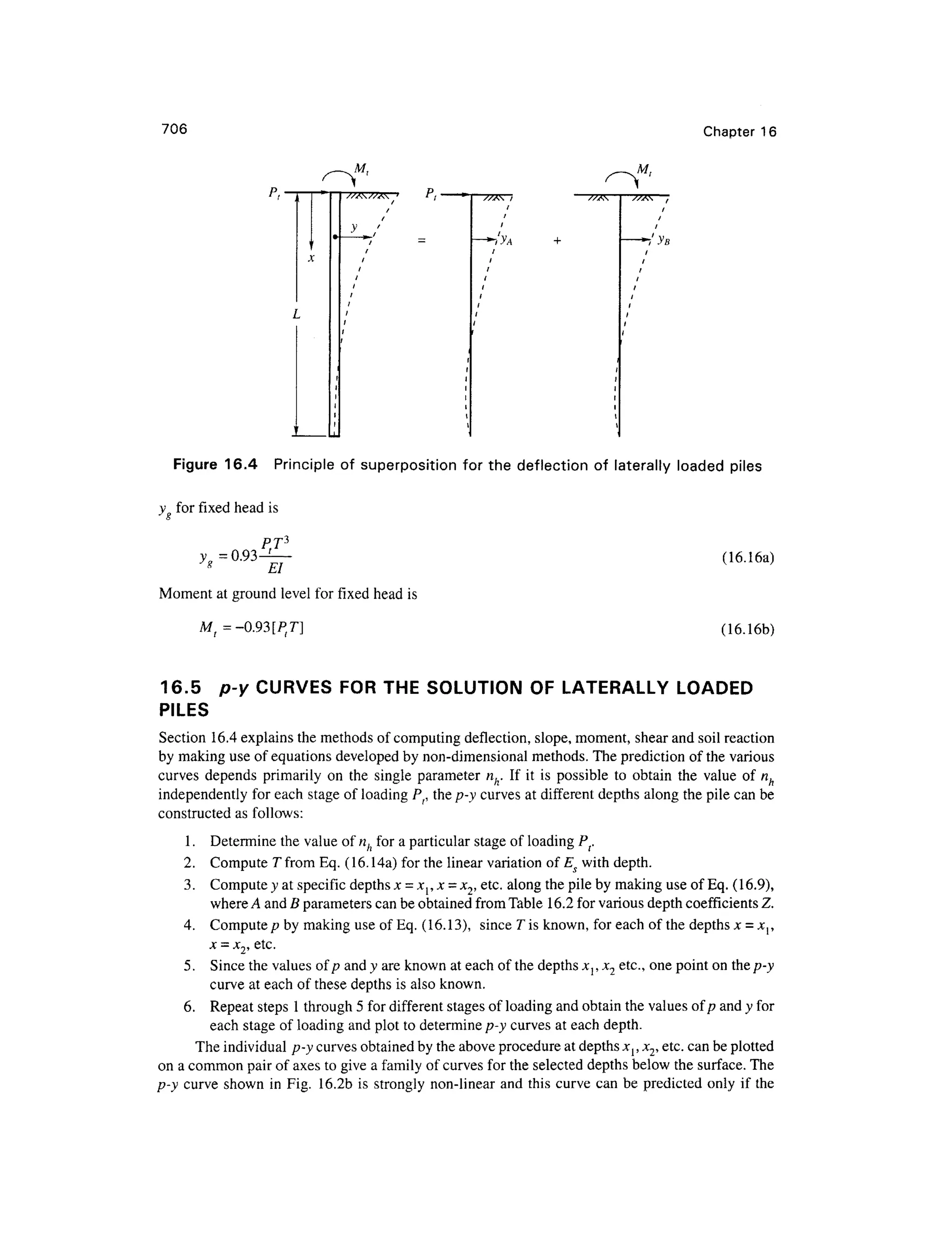
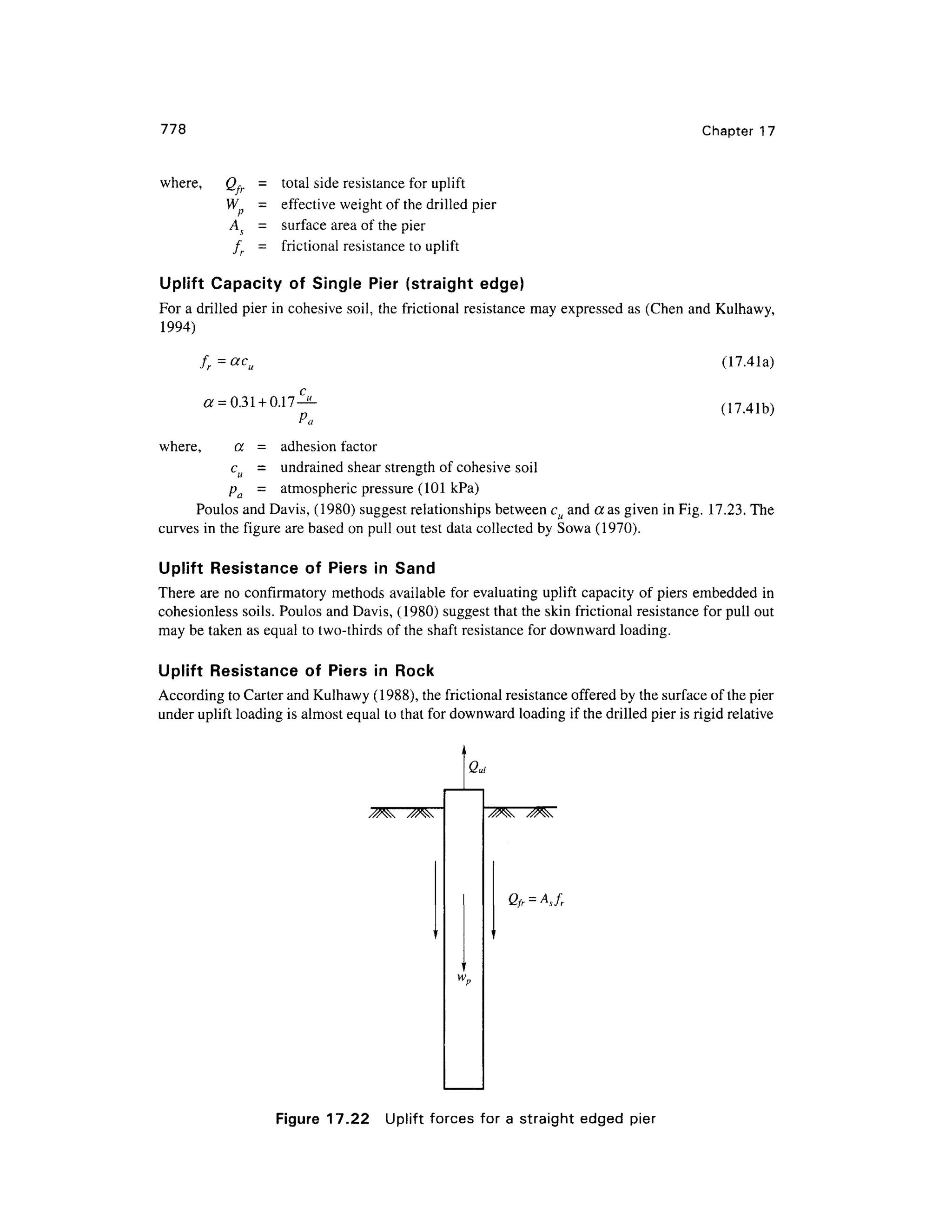
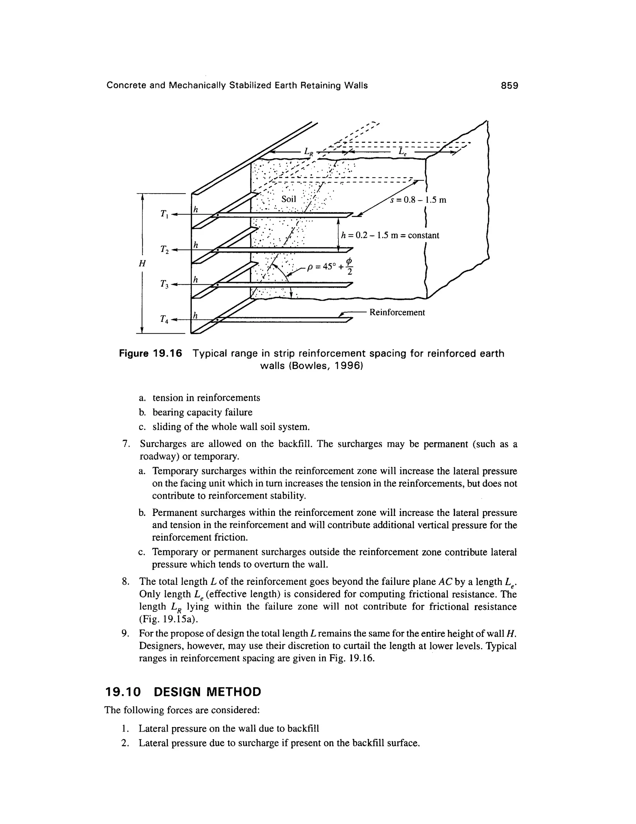
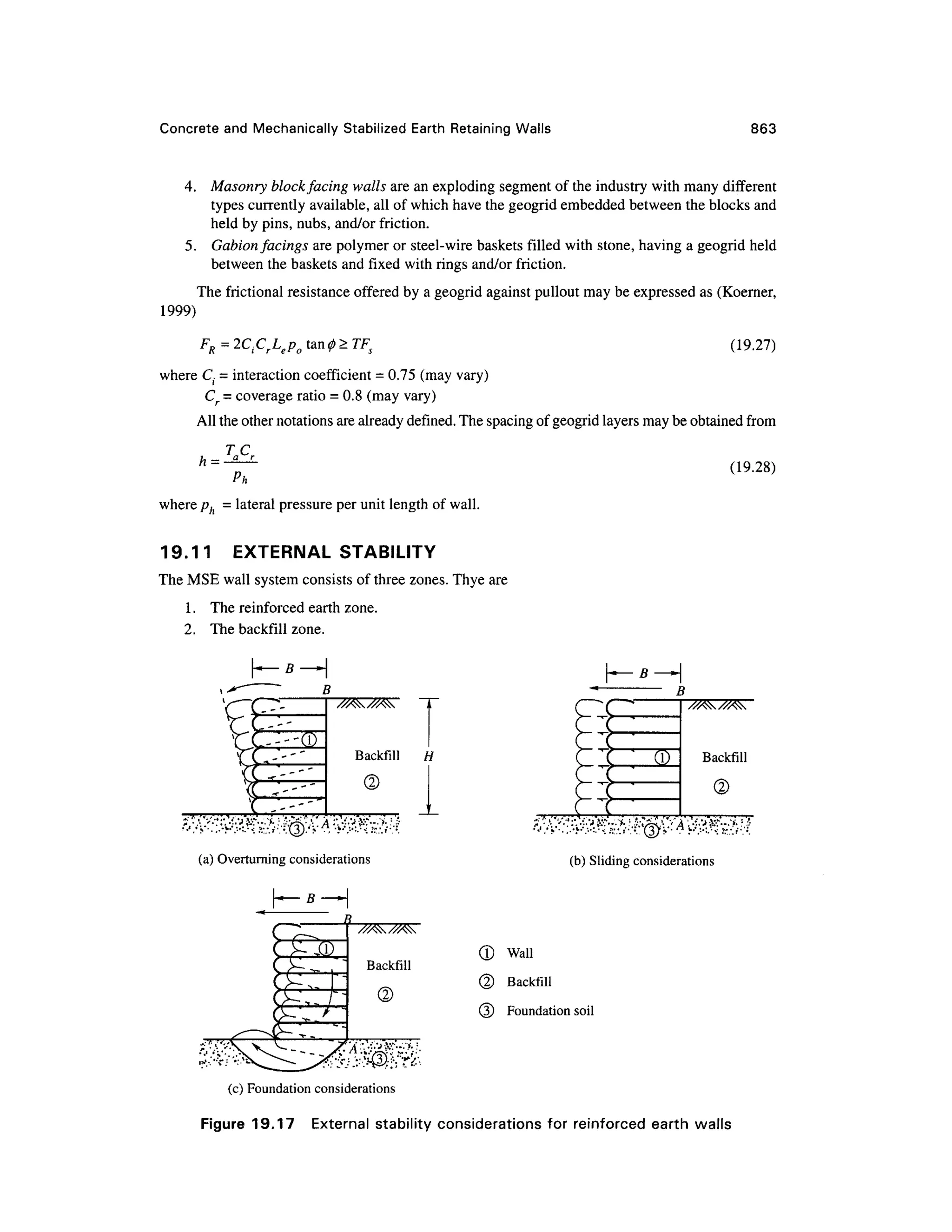
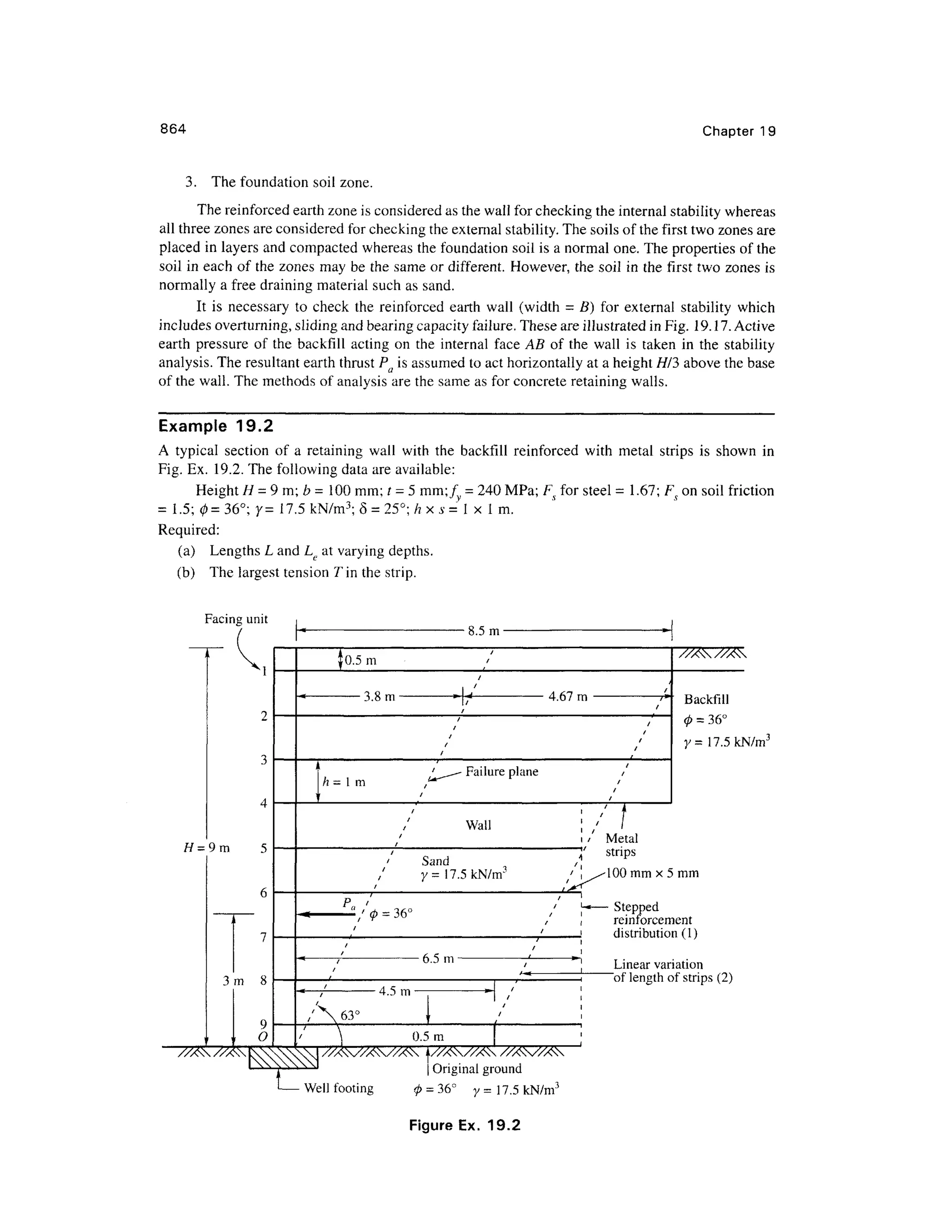
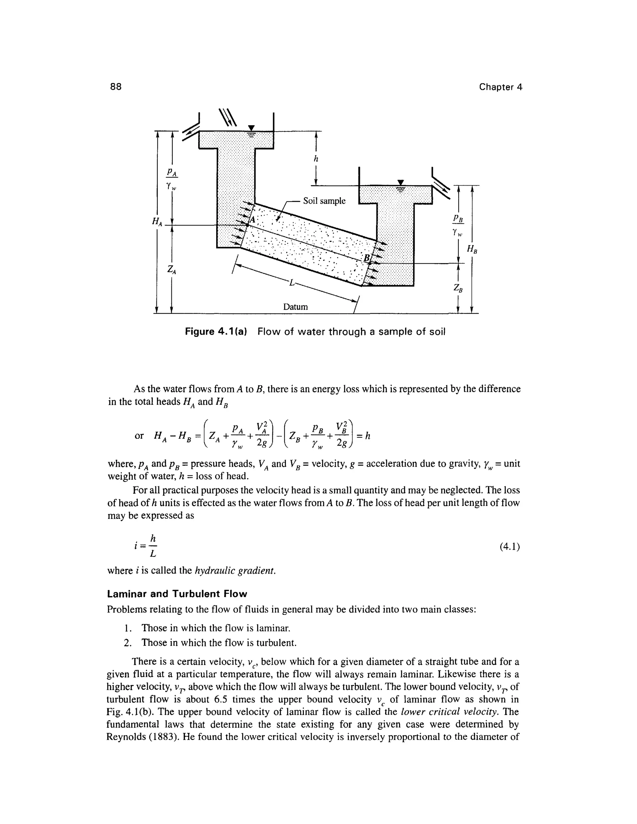
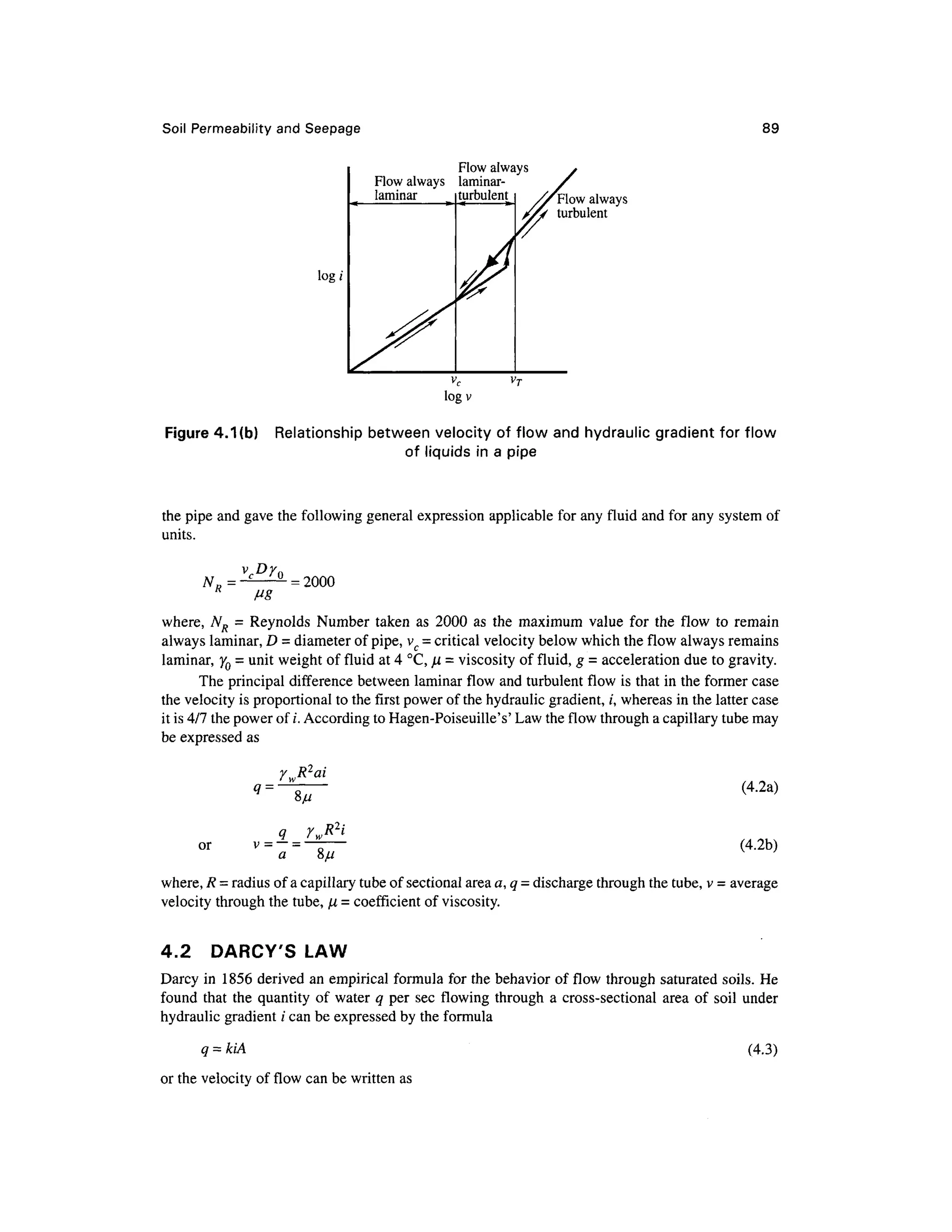
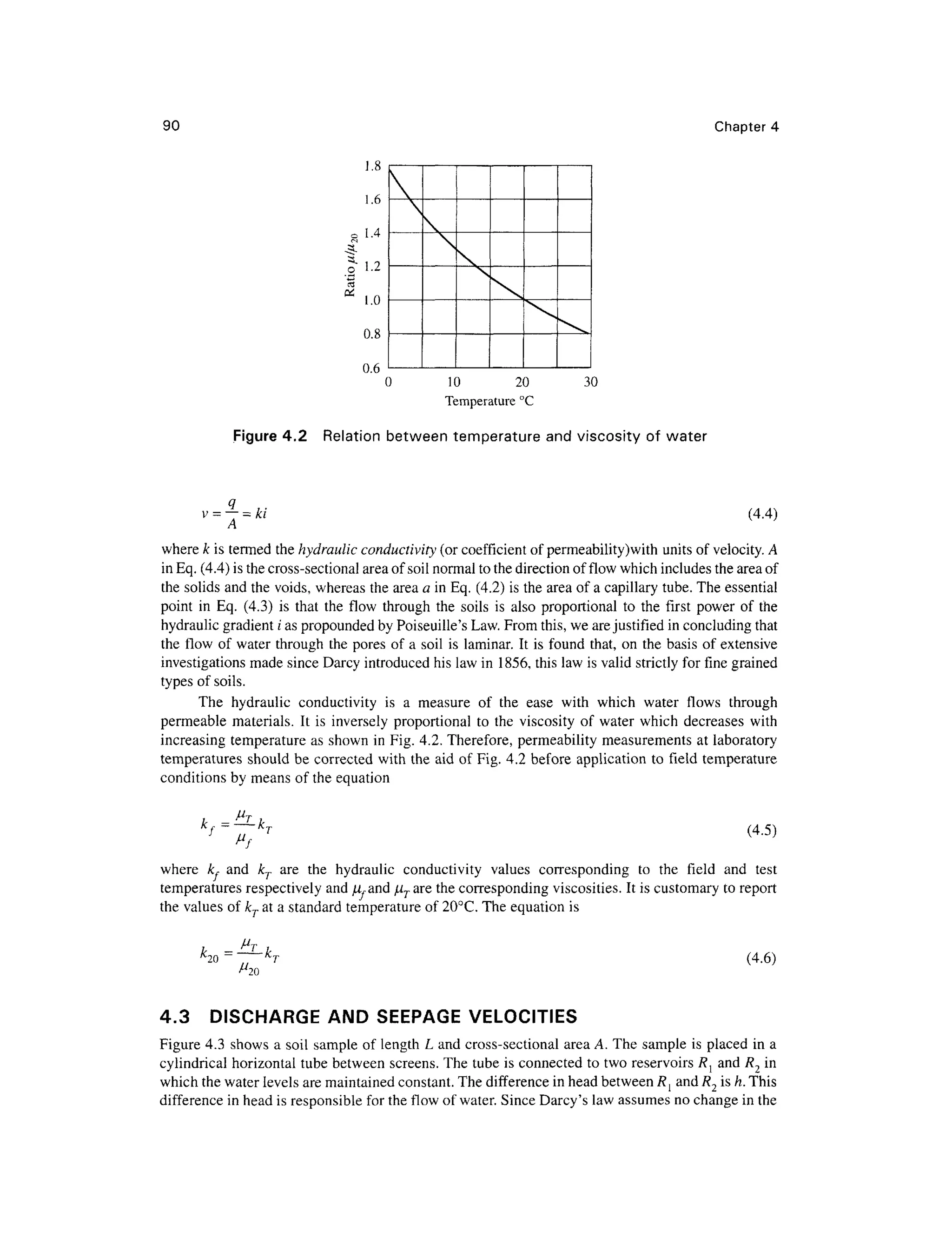
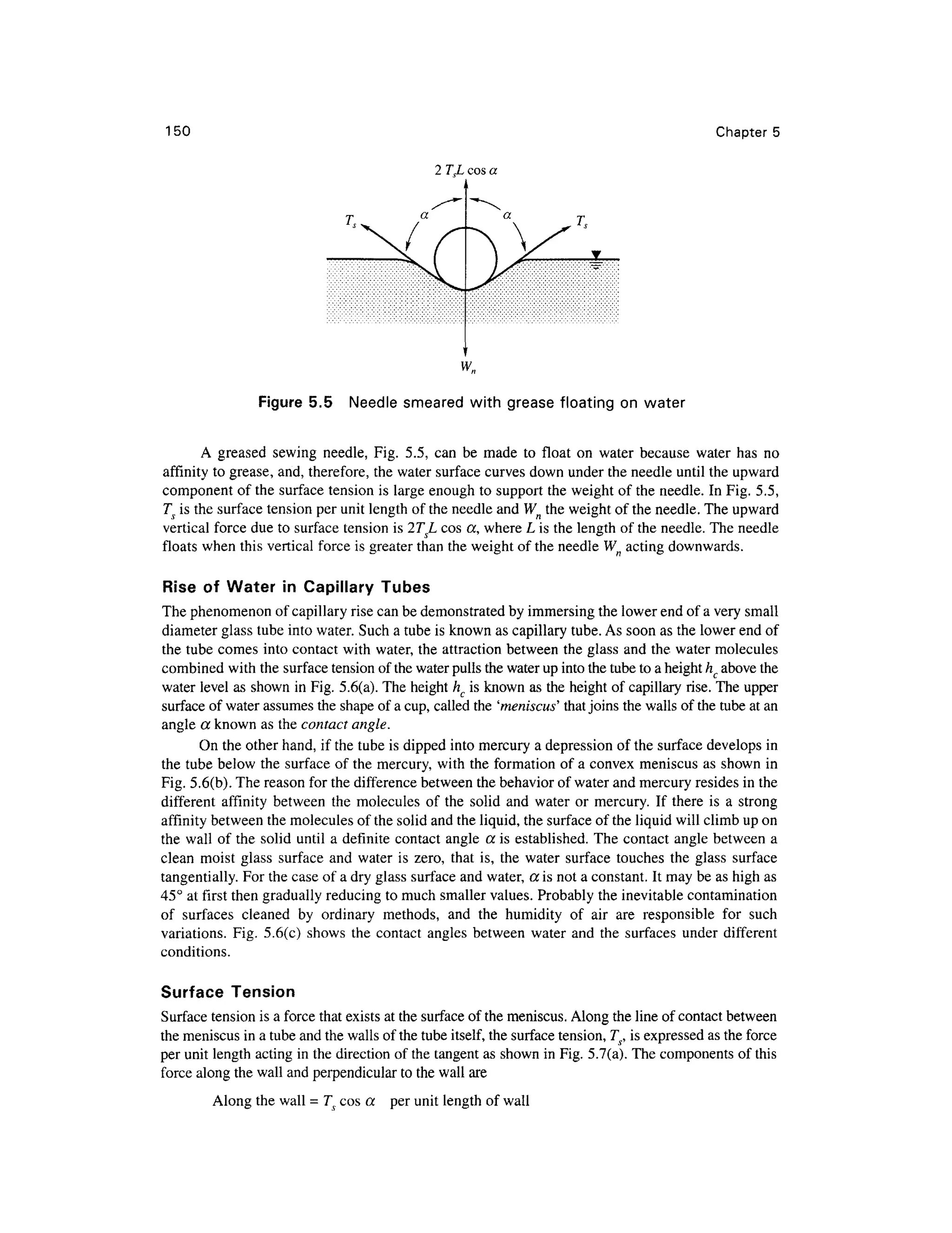
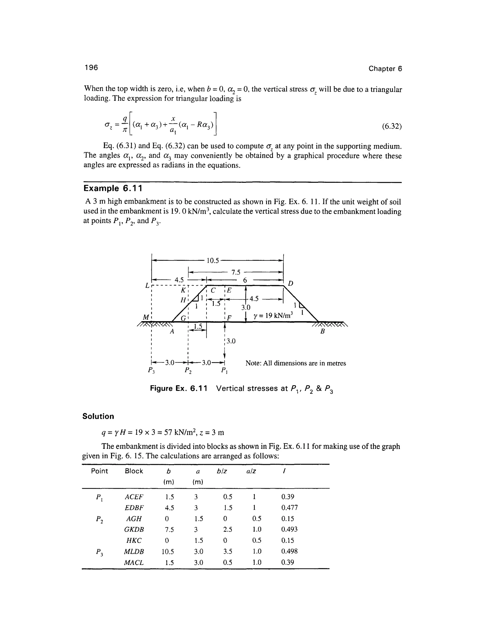
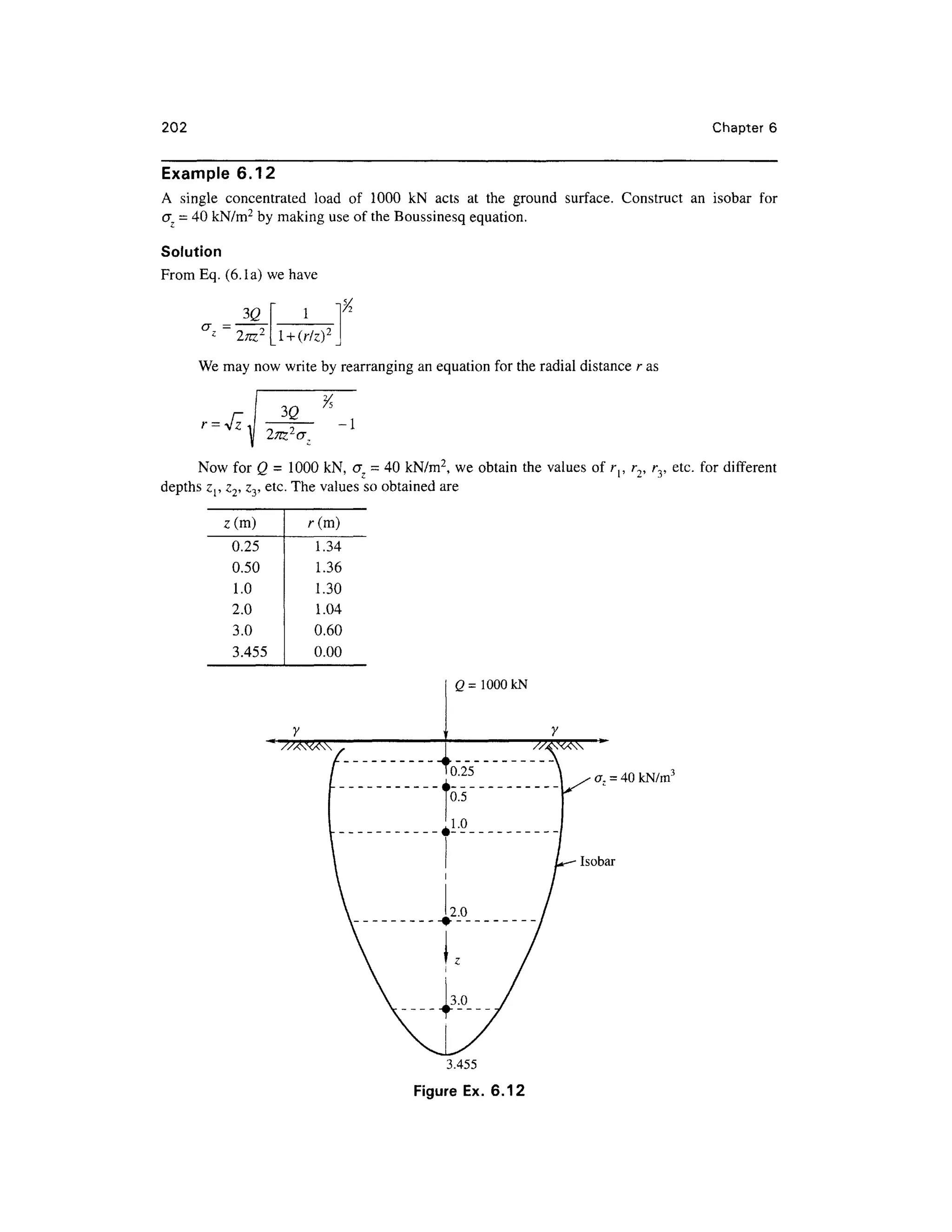
31. 1 2 Chapter 2
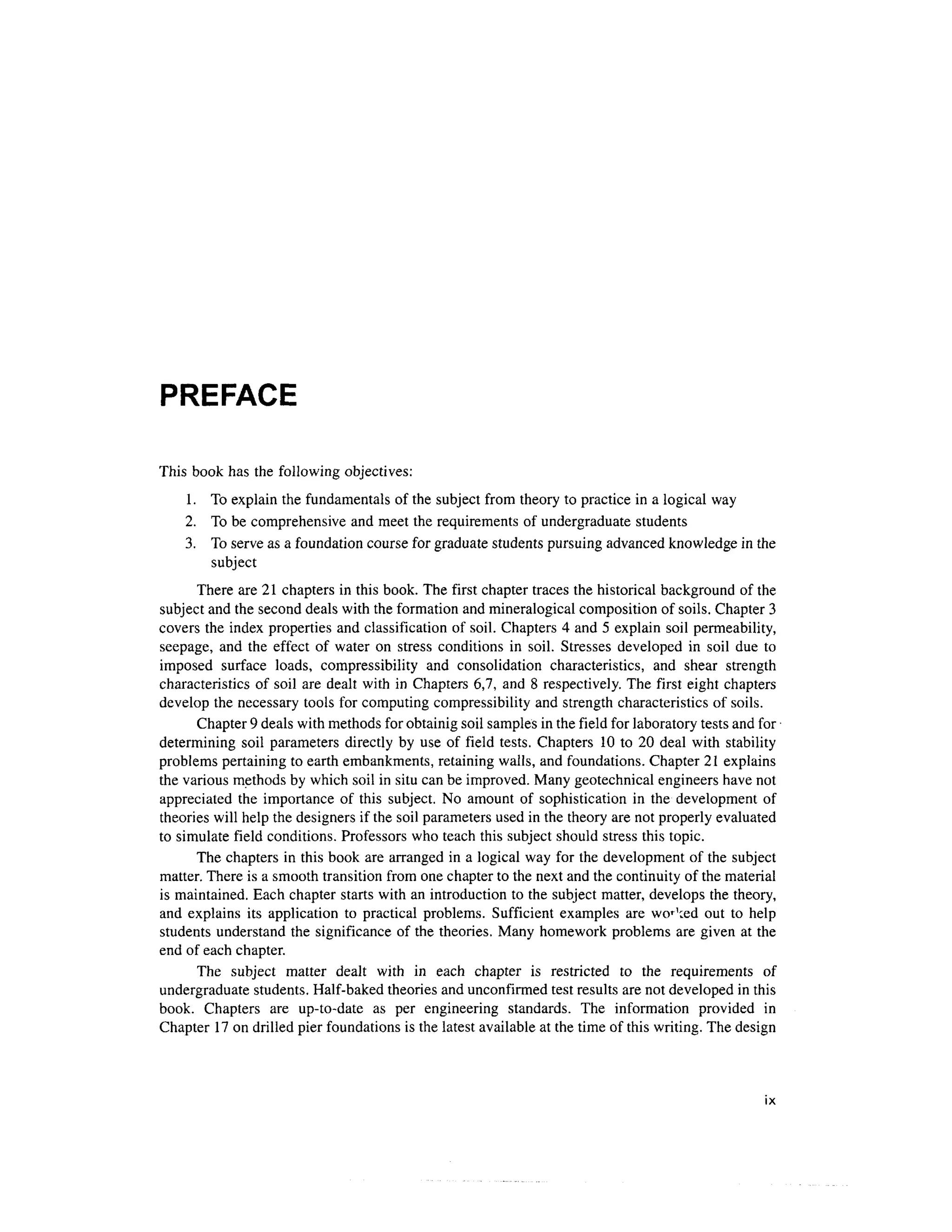
adjacent tetrahedra l unit . The sharin g of charge s leave s thre e negativ e charge s a t th e bas e per
tetrahedral unit and this along with two negative charges at the apex makes a total of 5 negative
charges to balance the 4 positive charges of the silicon ion. The process of sharing the oxygen ions
at the base with neighboring units leaves a net charge of -1 per unit.
The second building block is an octahedral unit with six hydroxyl ions at apices of an octahedral
enclosing an aluminum ion at the center. Iron or magnesium ions may replace aluminum ions in some
units. These octahedral units are bound together in a sheet structure with each hydroxyl ion common to
three octahedral units. This sheet is sometimes called as gibbsitesheet. The Al ion has 3 positive charges
and each hydroxyl ion divides its -1 charg e with two other neighboring units. This sharing of negative
charge with other units leaves a total of 2 negative charges per unit [(1/3) x 6]. The net charge of a unit
with a n aluminu m ion a t th e cente r is +1 . Fig. 2. 3 give s th e structura l arrangements o f the units.
Sometimes, magnesiu m replaces th e aluminu m atoms i n th e octahedra l unit s in thi s case , th e
octahedral sheet is called a brucite sheet.
Formation o f Mineral s
The combination of two sheets of silica and gibbsite in different arrangement s and conditions lead
to the formation of different clay minerals as given in Table 2.3. In the actual formation of the sheet
silicate minerals , the phenomenon of isomorphous substitution frequentl y occurs. Isomorphou s
(meaning same form) substitution consists of the substitution of one kind of atom for another.
Kaoiinite Minera l
This i s th e mos t commo n minera l o f th e kaoli n group . The buildin g blocks o f gibbsit e an d
silica sheets ar e arranged a s shown in Fig. 2.4 to give the structure of the kaolinite layer . The
structure i s compose d o f a singl e tetrahedra l shee t an d a singl e alumin a octahedra l shee t
combined i n unit s s o tha t th e tip s o f th e silic a tetrahedron s an d on e o f th e layer s o f th e
octahedral sheet form a common layer. All the tips of the silica tetrahedrons point in the same
direction and towards the center of the unit made of the silica and octahedral sheets. This gives
rise to strong ionic bonds between the silica and gibbsite sheets. The thickness of the layer is
about 7 A (on e angstro m = 10~ 8
cm) thick . The kaolinit e minera l i s formed b y stackin g th e
layers one above the other with the base of the silica sheet bonding to hydroxyls of the gibbsite
sheet b y hydroge n bonding . Sinc e hydroge n bond s ar e comparativel y strong , th e kaolinit e
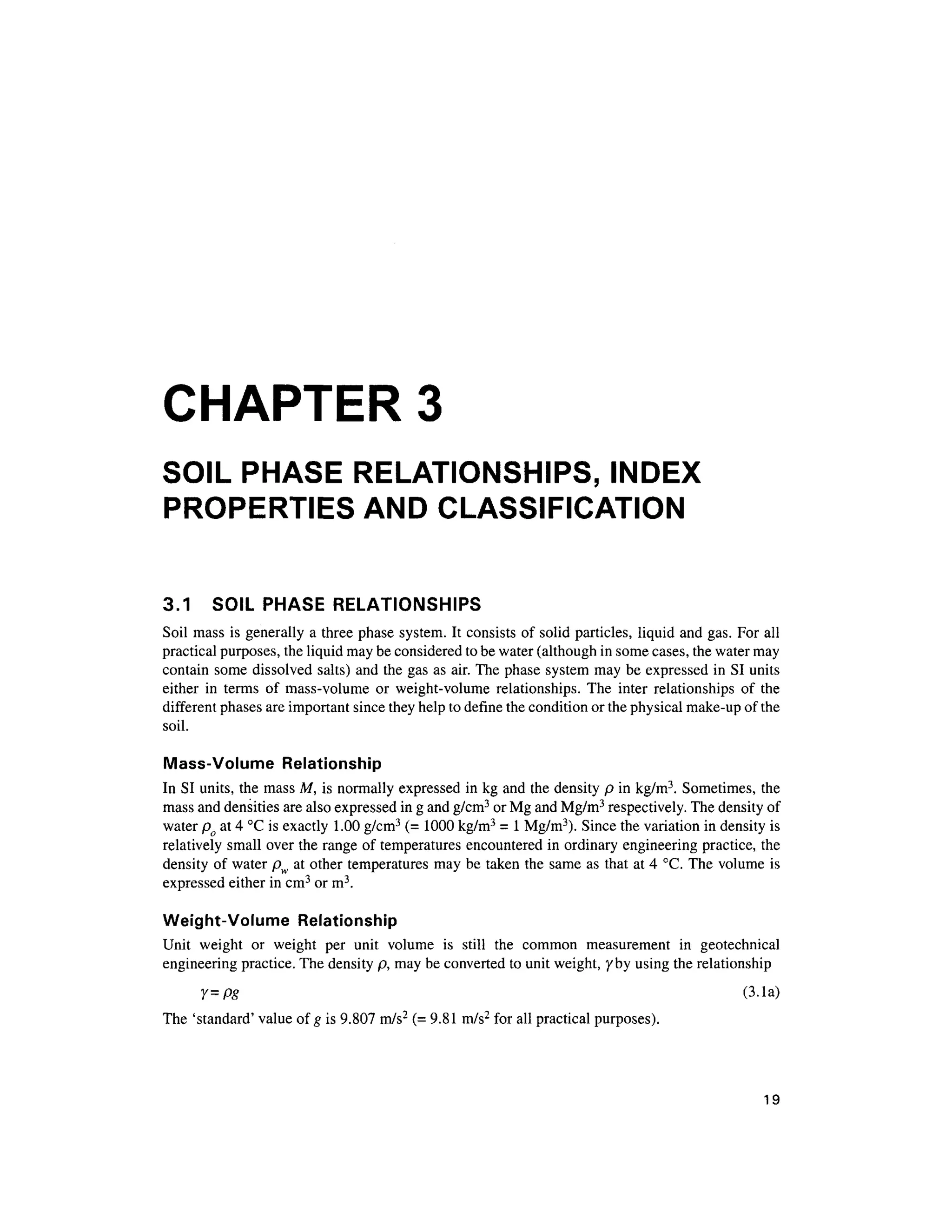
(a) Tetrahedral unit (b) Silica sheet
Silicons
Oxygen
]_ Symbolic representation
of a silica sheet
Figure 2.2 Basi c structural unit s in the silico n shee t (Grim , 1959 )

32. Soil Formatio n and Characterizatio n 13
(a) Octahedral uni t (b) Octahedral shee t
0 Hydroxyl s
I Symboli c representatio n
of a octahedral shee t
Aluminums,
magnesium or iron
Figure 2.3 Basi c structural unit s in octahedral sheet (Grim , 1959 )
crystals consist of many sheet stackings that are difficult t o dislodge. The mineral is therefore,
stable, an d wate r canno t ente r betwee n th e sheet s t o expan d th e uni t cells . Th e latera l
dimensions of kaolinite particles range from 100 0 t o 20,000 A and the thickness varie s fro m
100 to 100 0 A . In the kaolinite mineral there is a very small amount of isomorphous substitution.
Halloysite Minera l
Halloysite minerals are made up of successive layers with the same structural composition as those
composing kaolinite. In this case, however, the successive units are randomly packed and may be
separated by a single molecular layer of water. The dehydration of the interlayers by the removal of
the wate r molecules lead s t o change s in the properties o f the mineral. An importan t structural
feature of halloysite is that the particles appear to take tubular forms as opposed to the platy shape
of kaolinite.
Ionic bond
Hydrogen bon d
Gibbsite sheet
Silica shee t
T
7A
7A
7A
Figure 2.4 Structur e o f kaolinit e laye r

33. 14 Chapter 2
Montmorillonite Minera l
Montmorillonite i s th e mos t commo n minera l o f th e montmorillonit e group . Th e structura l
arrangement o f thi s minera l i s compose d o f tw o silic a tetrahedra l sheet s wit h a centra l alumin a
octahedral sheet . All the tips of the tetrahedra point in the same direction and toward the center of the
unit. The silica and gibbsite sheets are combined in such a way that the tips of the tetrahedrons of each
silica sheet and one of the hydroxyl layers of the octahedral sheet form a common layer . The atom s
common t o both the silica and gibbsite layer become oxyge n instead of hydroxyls. The thickness of
the silica-gibbsite-silica unit is about 10 A(Fig. 2.5). In stacking these combined units one above the
other, oxyge n layer s o f eac h uni t ar e adjacen t t o oxyge n o f th e neighborin g unit s wit h a
consequence tha t there i s a very weak bon d an d an excellent cleavage betwee n them . Wate r ca n
enter between the sheets, causing them to expand significantly and thus the structure can break into
10 A thic k structural units. Soils containin g a considerable amoun t o f montmorillonite mineral s
will exhibit high swelling and shrinkage characteristics. The lateral dimensions of montmorillonite
particles rang e fro m 100 0 t o 500 0 A wit h thicknes s varying from 1 0 to 5 0 A. Bentonit e cla y
belongs t o th e montmorillonit e group. I n montmorillonite , there i s isomorphou s substitutio n of
magnesium and iron for aluminum.
Illite
The basi c structura l uni t o f illit e is simila r t o tha t o f montmorillonit e excep t tha t som e o f th e
silicons are always replaced b y aluminum atoms and the resultant charge deficienc y is balanced by
potassium ions . Th e potassiu m ion s occu r betwee n uni t layers . Th e bond s wit h th e
nonexchangeable K +
ions are weaker than the hydrogen bonds, but stronger tha n the water bond of
montmorillonite. Illite , therefore , doe s no t swel l a s muc h i n th e presenc e o f wate r a s doe s
montmorillonite. Th e latera l dimension s o f illit e clay particle s ar e abou t th e sam e a s thos e o f
montmorillonite, 100 0 t o 500 0 A , bu t th e thicknes s o f illit e particle s i s greate r tha n tha t o f
montmorillonite particles, 50 to 500 A. The arrangement of silica and gibbsite sheets are as shown
in Fig. 2.6 .
2.8 CLA Y PARTICLE-WATE R RELATIONS
The behavior of a soil mass depends upon the behavior of the discrete particles composing th e mass
and th e patter n o f particl e arrangement . I n al l thes e case s wate r play s a n importan t part . Th e
Figure 2. 5 Structur e o f montmorillonit e laye r

34. Soil Formatio n an d Characterization 15
10A
T I I I I
T
loA
I I I I I I I I I I I I I I I I H T M — Potassium molecules
II I Mil I I I I I I III II I
1 1 1 1 1 1 1 1 1 1 1 1 I I 1 1 1 1 1 V«— Fairly strong bond
Silica sheet
Gibbsite sheet
Figure 2.6 Structur e o f illit e layer
behavior o f th e soi l mas s i s profoundly influence d by th e inter-particle-wate r relationships , th e
ability of the soil particles to adsorb exchangeable cations and the amount of water present.
Adsorbed Wate r j
The cla y particle s carr y a ne t negativ e charg e ^ n thei r surface . Thi s i s th e resul t o f bot h
isomorphous substitution and of a break in the continuity of the structure at its edges. The intensity
of the charge depend s t o a considerable exten t on tljie mineralogical characte r o f the particle. Th e
physical an d chemical manifestation s of the surfac e charge constitut e the surfac e activit y of the
mineral. Minerals ar e said to have high or low surface activity , depending on the intensity of the
surface charge. As pointed out earlier, the surface activity depends no t only on the specific surfac e
but also on the chemical and mineralogical composition of the solid particle. The surface activity of
sand, therefore, will not acquire all the properties of ^ true clay, even if it is ground to a fine powder.
The presenc e o f wate r doe s no t alte r it s properti e
changing it s unit weight. However, th e behavior o l
of coarse r fraction s considerabl y exceptin g
' a saturated soi l mas s consistin g o f fine san d
might chang e unde r dynamic loadings . Thi s aspec t o f the problem i s not considere d here . Thi s
article deals only with clay particle-water relations.
In nature every soil particle is surrounded by ^ater. Since the centers of positive and negative
charges of water molecules d o not coincide, the molecules behave like dipoles. The negative charge
on th e surfac e o f th e soi l particle , therefore , attract s th e positiv e (hydrogen ) en d o f th e wate r
molecules. The wate r molecules ar e arranged i n a definite pattern in the immediate vicinit y of the
boundary between solid and water. More than one layer of water molecules sticks on the surface with
considerable force and this attractive force decreases wit h the increase i n the distance o f the water
molecule from the surface. The electrically attracted water that surrounds the clay particle is known as
the diffused double-layer of water. The water located within the zone of influence is known as the
adsorbed layer as shown in Fig. 2.7. Within the zone of influence the physical properties of the water
are very different fro m those of free or normal water at the same temperature. Near the surface of the
particle the water has the property of a solid. At the middle of the layer it resembles a very viscous
liquid and beyond the zone of influence, the propenles of the water become normal. The adsorbe d
water affects the behavior of clay particles when subjected to external stresses, since it comes between
the particle surfaces. To drive off the adsorbed water , the clay particle mus t be heated to more than
200 °C, whic h woul d indicat e tha t th e bon d betwee n th e wate r molecule s an d th e surfac e i s
considerably greater than that between normal water molecules.

35. 16
Particle surfac e
Chapter 2
Adsorbed
water
Distance
Figure 2. 7 Adsorbe d wate r laye r surrounding a soil particl e
The adsorbed film of water on coarse particles is thin in comparison wit h the diameter o f the
particles. In fine grained soils, however, this layer of adsorbed water is relatively much thicker and
might even exceed th e size of the grain. The forces associate d wit h the adsorbed layer s therefor e
play an important part in determining the physical properties of the very fine-grained soils, but have
little effect o n the coarser soils .
Soils in which the adsorbed film is thick compared to the grain size have properties quite different
from othe r soil s havin g th e sam e grai n size s bu t smalle r adsorbe d films . Th e mos t pronounce d
characteristic o f the forme r is their ability to deform plasticall y without cracking whe n mixed wit h
varying amounts of water. This is due to the grains moving across one another supported by the viscous
interlayers of the films. Such soils are called cohesive soils, for they do not disintegrate with pressure but
can be rolled into threads with ease. Here the cohesion is not due to direct molecular interaction between
soil particles at the points of contact but to the shearing strength of the adsorbed layers that separate the
grains at these points.
Base Exchang e
Electrolytes dissociat e whe n dissolve d i n wate r int o positivel y charge d cation s an d negativel y
charged anions . Acids break up into cations of hydrogen and anions such as Cl or SO4. Salts and
bases split into metallic cations such as Na, K or Mg, and nonmetallic anions. Even water itself is an
electrolyte, because a very small fraction of its molecules always dissociates into hydrogen ions H+
and hydroxyl ions OH". These positively charged H+
ions migrate to the surface of the negatively
charged particle s and form what is known as the adsorbed layer . These H+
ions can be replaced by
other cations such as Na, K or Mg. These cation s enter the adsorbed layer s and constitute what is
termed a s an adsorption complex. The process of replacing cations of one kind by those of another
in an adsorption comple x is known as base exchange. B y base exchange is meant the capacity of

36. Soil Formation and Characterization 1 7
Table 2. 4 Exchang e capacity o f som e clay mineral s
Mineral group Exchang e capacity (meq per 10 0 g)
Kaolinites 3. 8
Illites 4 0
Montmorillonites 8 0
Table 2.5 Cation s arranged in the orde r of decreasing shear strength of clay
NH/ > H+
> K+
> Fe+++
>A1+++
> Mg+
> Ba++
> Ca++
> Na+
> Li+
colloidal particle s to change the cations adsorbed o n their surface. Thus a hydrogen clay (colloi d
with adsorbed H cations) can be changed to sodium clay (colloid wit h adsorbed N a cations) by a
constant percolation of water containing dissolved Na salts. Such changes can be used to decrease
the permeability of a soil. Not all adsorbed cations are exchangeable. The quantity of exchangeable
cations in a soil is termed exchange capacity.
The base exchange capacity is generally defined in terms of the mass of a cation which may
be held on the surface of 100 gm dry mass of mineral. It is generally more convenient to employ a
definition o f base exchange capacity in milli-equivalents (meq) per 10 0 gm dry soil. One meq is
one milligra m o f hydroge n o r th e portio n o f an y io n whic h wil l combin e wit h o r displac e
1 milligram of hydrogen.
The relative exchange capacity of some of the clay minerals is given in Table 2.4.
If one element, suc h as H, Ca, or Na prevails over the other in the adsorption comple x o f a
clay, the clay i s sometimes give n the name of this element, fo r example H-cla y or Ca-clay. The
thickness and the physical properties of the adsorbed film surrounding a given particle, depend to a
large extent on the character of the adsorption complex. These films are relatively thick in the case
of strongly water-adsorbent cations such as Li+
and Na+
cations but very thin for H+
. The films of
other cations have intermediate values. Soils with adsorbed Li+
and Na+
cations are relatively more
plastic at low water contents and possess smaller shear strength because the particles are separated
by a thicker viscous film. The cations in Table 2.5 are arranged in the order o f decreasing shea r
strength of clay.
Sodium clays in nature are a product either of the deposition of clays in sea water or of their
saturation by saltwater flooding or capillary action. Calcium clays are formed essentially by fres h
water sediments. Hydroge n clay s are a result of prolonged leachin g o f a clay by pur e or acidi c
water, with the resulting removal of all other exchangeable bases.
2.9 SOI L MASS STRUCTURE
The orientation of particles in a mass depends on the size and shape of the grains as well as upon
the mineral s o f whic h th e grain s ar e formed . Th e structur e of soil s tha t i s forme d b y natural
deposition ca n b e altere d b y externa l forces . Figur e 2.8 gives the variou s type s o f structure s of
soil. Fig. 2.8(a) is a single grained structure whic h is formed by the settlement of coarse grained
soils in suspension in water. Fig. 2.8(b ) is a flocculentstructure forme d by th e deposition o f the
fine soi l fractio n i n water . Fig . 2.8(c ) i s a honeycomb structure whic h i s forme d b y th e
disintegration o f a flocculen t structur e unde r a superimpose d load . Th e particle s oriente d i n a
flocculent structur e wil l hav e edge-to-fac e contac t a s show n i n Fig . 2.8(d) wherea s i n a

37. Chapter 2
(a) Single grain structure (b) Flocculent structure (c) Honeycomb structure
(d) Flocculated typ e structure
(edge to face contact)
(e) Dispersed structure
(face to face contact)
(f) Undisturbed salt water deposit (g ) Undisturbed fresh wate r deposit
Figure 2. 8 Schemati c diagram s o f various type s of structures (Lambe , 1 958a)
honeycomb structure , the particles will have face-to-face contac t as shown i n Fig. 2.8(e). Natural
clay sediment s wil l hav e mor e o r les s flocculate d particl e orientations . Marine clay s generall y
have a more open structur e than fresh water clays. Figs. 2.8(f) an d (g) show th e schematic views
of salt water and fres h water deposits.

38. CHAPTER 3
SOIL PHASE RELATIONSHIPS, INDEX
PROPERTIES AND CLASSIFICATION
3.1 SOI L PHAS E RELATIONSHIP S
Soil mass i s generally a three phase system . It consists of solid particles, liqui d and gas. For all
practical purposes, the liquid may be considered to be water (although in some cases, the water may
contain some dissolve d salts ) and the gas as air. The phase system may be expressed i n SI units
either i n term s o f mass-volum e o r weight-volum e relationships . Th e inte r relationship s o f th e
different phases are important since they help to define the condition or the physical make-up of the
soil.
Mass-Volume Relationshi p
In SI units, the mass M, i s normally expressed i n kg and the density p i n kg/m3
. Sometimes, th e
mass and densities are also expressed i n g and g/cm3
or Mg and Mg/m3
respectively. The density of
water po a t 4 °C is exactly 1.0 0 g/cm3
(= 1000 kg/m3
= 1 Mg/m3
). Since the variation in density is
relatively small over the range of temperatures encountered in ordinary engineering practice, th e
density of water pw a t other temperature s ma y be taken the same a s that at 4 °C. The volum e is
expressed eithe r in cm3
or m3
.
Weight-Volume Relationshi p
Unit weigh t o r weigh t pe r uni t volum e i s stil l th e commo n measuremen t i n geotechnica l
engineering practice. The density p, may be converted to unit weight, 7by using the relationship
Y=pg (3.la )
The 'standard ' value of g is 9.807 m/s2
(= 9.81 m/s2
for all practical purposes) .
19

39. 20 Chapter 3
Conversion o f Densit y o f Water pw t o Uni t Weight
From Eq. (3.la)
•W ~ ^VV °
Substituting pw = 1000 kg/m3
and g = 9.81 m/s2
, we have
r= 1000^9.81^1=9810^
m3
s 2
/ m 3
s2
1 kg-m
Since I N (newton) = — , w e have,
rrr nr
cm-
I S 1
or 7 , = lx—s — x 9.81 =9.81 kN/m3
In general, the unit weight of a soil mass may be obtained from the equation
y=9.81pkN/m3
(3.If )
where in Eq. (3. If), p is in g/cm3
. For example, if a soil mass has a dry density, pd = 1.7 g/cm3
, the
dry unit weight of the soil is
7^=9.81 x 1.7 = 16.6 8 kN/m3
(3.1g )
3.2 MASS-VOLUM E RELATIONSHIP S
The phase-relationships in terms of mass-volume and weight-volume for a soil mass are shown by a block
diagram in Fig. 3.1. A block of unit sectional area is considered. The volumes of the different constituents
are shown on the right side and the corresponding mass/weights on the right and left sides of the block. The
mass/weight of air may be assumed as zero.
Volumetric Ratio s
There are three volumetric ratios that are very useful i n geotechnical engineering and these can be
determined directly from the phase diagram, Fig. 3.1.
Weight Volume
W
Air
Water
Solids
Mass
Mu
M
Figure 3.1 Bloc k diagram—three phase s of a soil elemen t

40. Soil Phas e Relationships, Inde x Propertie s and Soil Classificatio n 2 1
(3.2)
1. Th e void ratio, e, is defined as
«=^
S
where, V v = volume of voids, and Vs = volume of the solids .
The void ratio e is always expressed a s a decimal.
2. Th e porosity n is defined as
Vv
v__ - I (CG1 / O O
n — x luu /o {->•->)
where, V -tota l volume of the soil sample.
The porosity n is always expressed a s a percentage.
3. Th e degree of saturation S is defined as
5 =
^LX100% (34 )
v
where, V w = volume of water
It is always expressed a s a percentage.When S = 0%, the soil is completely dry , and when
S = 100%, th e soil is fully saturated .
Mass-Volume Relationships
The othe r aspect s o f th e phas e diagra m connecte d wit h mass o r weigh t ca n b e explaine d with
reference to Fig. 3.1.
Water Content , w
The water content, w, of a soil mass is defined as the ratio of the mass of water, Mw, in the voids to
the mass of solids, Ms, as
M
The water content, which is usually expressed as a percentage, can range from zero (dry soil) to
several hundred percent. The natural water content for most soils is well under 100%, but for the soils of
volcanic origin (for example bentonite) it can range up to 500% or more.
Density
Another ver y usefu l concep t i n geotechnical engineerin g i s density (or , uni t weight ) whic h i s
expressed a s mas s pe r uni t volume. Ther e ar e several commonl y use d densities . Thes e ma y be
defined as the total (or bulk), or moist density, pr; the dry density, pd; the saturated density, psat; the
density of the particles, solid density, ps; and density of water pw. Each of these densities is defined
as follows with respect t o Fig. 3.1.
M
Total density, p t = — (3.6 )

41. 22 Chapte r 3
s
Dry density, p d = -y
- (3.7 )
M
Saturated density, /? sat = — (3.8 )
forS= 100 %
M?
Density of solids, p s = — -
(3.9 )
Mw
Density of water, P w
=
~77L
(3.10 )
w
Specific Gravit y
The specific gravity of a substance is defined as the ratio of its mass in air to the mass of an equal
volume of water at reference temperature, 4 °C. The specific gravity of a mass of soil (including air,
water and solids) is termed as bulk specific gravity Gm. It is expressed a s
r -?< - M
™
The specific gravity of solids, Gs, (excluding air and water) is expressed b y
_ P, _ M
, (3J2)
Interrelationships o f Differen t Parameter s
We can establish relationships between the different parameters defined by equations from (3.2) through
(3.12). In order to develop the relationships, the block diagram Fig. 3.2 is made use of. Since the sectional
area perpendicular to the plane of the paper is assumed as unity, the heights of the blocks will represent
the volumes. The volum e of solids may be represented as V s = 1 . When the soil is fully saturated , the
voids are completely filled with water.
Relationship Betwee n e an d n (Fig . 3.2 )
1-n
l + e
(3.13)
Relationship Betwee n e, G s and S
Case 1: When partially saturated (S < 100%)
p

42. Soil Phas e Relationships , Inde x Propertie s an d Soil Classificatio n 23
wG wG
Therefore, 5 = - o r e=- (3.14a)
Case 2: When saturated (S = 100%)
From Eq. (3.14a), we have (for 5=1)
e = wG. (3.14b)
Relationships Betwee n Densit y p an d Other Parameter s
The density of soil can be expressed in terms of other parameters for cases of soil (1) partially
saturated (5 < 100%); (2) fully saturate d (S = 100%); (3) Fully dry (S = 0); and (4) submerged.
Case 1 : For S < 100%
=
Pt
~
V l + el + e
From Eq. (3.1 4a) w = eS/Gs; substitutin g for w in Eq. (3.15), we have
p
'=
1 «
Case 2: For S=100%
From Eq. (3.16)
Case 3: For S = 0%
FromEq. (3.16)
l + e
(3.15)
(3.16)
(3.17)
(3.18)
Weight
W
Air
Water
Volume
Solids
I
V
V=e
-V= l+e
Mass
M
Figure 3.2 Bloc k diagram—three phases of a soil elemen t

43. 24 Chapte r 3
Case 4: When the soil is submerged
If the soil is submerged, th e density of the submerged soi l pb, is equal to the density of the
saturated soil reduced b y the density of water, that is
p (G + e)p
EsJ
-- £s
Relative Densit y
The looseness or denseness of sandy soil s can be expressed numericall y b y relative density D r,
defined by the equation
D
r= e
e
maX
~l * 10Q
(3.20 )
max mi n
in which
emax= voi d ratio of sand in its loosest state having a dry density of p dm
e
mm =VO
^ ra
ti° m
its
densest stat e having a dry density of pdM
e
= voi d ratio under in-situ condition having a dry density of p d
From Eq. (3.18), a general equation for e may be written as
Pd
Now substituting the corresponding dry densities for emax, em-m and e in Eq. (3.20) and simplifying,
we have
n _ PdM v Pd ~Pdmi m
U — A A 1 JJ/" 5 O 1
r
o o - o U-^ 1
)
rd VdM ^dm
The loosest state for a granular material can usually be created by allowing the dry material to
fall into a container from a funnel hel d in such a way that the free fall is about one centimeter. The
densest state can be established by a combination of static pressure and vibration of soil packed in
a container.
ASTM Test Designation D-2049 (1991) provides a procedure fo r determining the minimum
and maximu m dry uni t weight s (o r densities) o f granular soils. Thi s procedur e ca n b e use d fo r
determining Dr in Eq. (3.21).
3.3 WEIGHT-VOLUM E RELATIONSHIP S
The weight-volume relationships can be established from the earlier equations by substituting yfor
p and W for M. The various equations are tabulated below.
W
1. Wate r content w = -j^L
xlOO (3.5 a)
s
W
2. Tota l unit weight ^ =
17 (3.6a )
Ws
3. Dr y unit weight y d
= —j- (3.7a )

44. Soil Phas e Relationships , Inde x Propertie s and Soil Classification 2 5
W
4. Saturate d unit weight y sal = —(3.8a )
W
s
5. Uni t weight of solids y f
s
=
~y~ (3.9a )
w
6. Uni t weight of water YW =
~V~~ (3.10a )
w
W
1. Mas s specific gravity G = -
(3. 1 la)
' w
W
si _ S
8. Specifi c gravity of solids s
~Vv (3.12a )
s'w
G Y ( 1 +w)
9. Tota l unit weight for 5< 10
0 y =-£^z -
(3.15a )
or 1 +e
Y (G +e)
10. Saturate d unit weight Y^
= — —- -
(3.17a )
1 +e
Y G
11. Dr y uni t weight y d = -!K
—*- (3 . 18a)
1 + e
Y ( G -1 )
12. Submerge d unit weight Yh
= — —- -
(3.19a )
l + e
n _ Y dM „ Yd ~ Y dm
13. Relativ e density r
~T~ v T ^ (3.21a )
'd idM f dm
3.4 COMMENT S O N SOIL PHAS E RELATIONSHIP S
The void ratios of natural sand deposits depend upon the shape of the grains, the uniformity of
grain size, and the conditions of sedimentation. The void ratios of clay soils range from less than
unity to 5 or more. The soils with higher void ratios have a loose structure and generally belong
to the montmorillonite group. The specific gravity of solid particles of most soils varies from 2.5
to 2.9. For most of the calculations, G ca n be assumed as 2.65 for cohesionless soils and 2.70 for
5
clay soils. The dr y unit weights (yd) o f granular soils range from 1 4 to 1 8 kN/m3
, whereas, th e
saturated unit weights of fine grained soils can range from 12.5 to 22.7 kN/m 3
. Table 3.1 gives
typical values of porosity, void ratio, water content (when saturated) and unit weights of various
types of soils.

45. 26 Chapter 3
Table 3. 1 Porosity , voi d ratio, water content , and unit weights of typical soils i n
natural stat e
Soil
no.
1
1
2
3
4
5
6
7
8
9
10
Description o f soi l
2
Uniform sand , loos e
Uniform sand , loos e
Mixed-grained sand , loos e
Mixed-grained sand , dens e
Glacial till , mixed grained
Soft glacia l clay
Soft glacia l clay
Soft slightl y organic clay
Soft highl y organic clay
Soft bentonit e
Porosity
n
%
3
46
34
40
30
20
55
37
66
75
84
Void
ratio
e
4
0.85
0.51
0.67
0.43
0.25
1.20
0.60
1.90
3.00
5.20
Water
content
w%
5
32
19
25
16
9
45
22
70
110
194
Unit weight
kN/m3
rd
6
14.0
17.0
15.6
18.2
20.8
11.9
16.7
9.1
6.8
4.2
'sat
7
18.5
20.5
19.5
21.2
22.7
17.3
20.3
15.5
14.0
12.4
Example 3. 1
A sampl e o f we t silt y clay soi l ha s a mas s o f 12 6 kg. Th e followin g data wer e obtaine d fro m
laboratory test s on the sample: Wet density, pt = 2.1 g/cm3
, G = 2.7, water content, w - 15% .
Determine (i ) dry density, pd, (ii ) porosity, (iii) void ratio, and (iv) degree of saturation.
Solution
Mass of sample M = 126 kg.
Volume V =
126
= 0.06 m
2.1 xlO3
Now, M s + Mw = M, o r M y + wMy = M?(l + w) = M
Therefore, M. = -^—= -— = 109.57 kg ; M ,= M
^ l + w 1.1 5H s= 16.43 k g
Volume Mass
Air
Water
Solids-
M,.
M,
M
Figure Ex . 3. 1

46. Soil Phas e Relationships , Inde x Propertie s an d Soil Classification 2 7
Now, V == = 0.01643 m 3
;
w
p w 100 0
= 0.04058
Gspw 2.7x100 0
= V-V=0.06000 -0.04058 =0.01942 m 3
.
(i) Dr y density, /?.= —* - =
= 1826.2 kg/m 3
j ^ ^ y 0.0 6
(ii) Porosity , n^xlOO~ ft01942xl0
° = 32.37%
V 0.0 6
(iii) Voi d ratio, e = ^-
=Q
-01942
=0.4786
V; 0.0405 8
(i v) Degre e of saturation, S = -*
- x1 00 = °'01 43
x 1 00 = 84.6%
V. 0.0194 2
Example 3. 2
Earth is required to be excavated from borrow pits for building an embankment. The wet unit weight
of undisturbed soil is 1 8 kN/m3
and its water content is 8%. In order to build a 4 m high embankment
with top width 2 m and side slopes 1:1 , estimate the quantity of earth required to be excavated per
meter length of embankment. Th e dry unit weight required in the embankment i s 15 kN/m3
with a
moisture content of 10% . Assume the specific gravity of solids a s 2.67. Also determin e th e void
ratios and the degree o f saturation of the soil in both the undisturbed and remolded states .
Solution
The dry unit weight of soil in the borrow pit is
7, = -£
- =— = 16.7 kN/m 3
d
l + w1.0 8
Volume of embankment per meter length Ve
2
The dry unit weight of soil in the embankment is 15 kN/m3
2m — |
Figure Ex. 3. 2

47. 28 Chapte r 3
Volume of earth required to be excavated V pe r meter
V= 24 x
— = 21.55m3
16.7
Undisturbed state
V = -^- = — x— = 0.64 m 3
; V = 1-0.6 4 = 0.36 m 3
5
Gj w 2.6 7 9.8 1
n^^>
e = —-=0.56, W = 18.0-16. 7 = 1.3 kN
0.64
V
Degree of saturation, S = — —x 100 , wher e
V
= 0.133 m3
9.8i
Now, £ = -9^x100 =36.9%
0.36
Remolded state
V = -^ - = -
- -
=0.57 m3
s
Gy w 2.67x9.8 1
yv= 1-0.57 = 0.43 m 3
0.43
e = = 0.75; 7 , = yd (1 +w) = 15 x 1.1 = 16.5 kN/m 3
0.57
Therefore, W = 16.5-15. 0 = 1.5 kN
Vw = —= 0.153 m3
w
9.8 1
0.43
Example 3. 3
The moistur e conten t of a n undisturbed sample o f clay belonging t o a volcanic region i s 265%
under 100 % saturation. The specifi c gravity of the solids is 2.5. The dr y unit weight is 21 Ib/ft 3
.
Determine (i ) the saturated unit weight, (ii) the submerged unit weight, and (iii) void ratio.
Solution
(i) Saturated unit weight, ysat = y
W=W + W = w W + W = W ( l + w)
w s a s s ^ '
W W
From Fig. Ex. 3.3, Yt= — = —=W. Henc e

48. Soil Phas e Relationships, Inde x Propertie s and Soil Classificatio n 29
V = l
Water
W=Y,
Figure Ex. 3. 3
Yt = 21(1 +2.65) = 21 x3.65 = 76.65 lb/ft 3
(ii) Submerged unit weight, yb
Yb = ^sat -Yw = 76.65 - 62.4 = 14.25 lb/ft 3
(iii) Void ratio, e
V = -^
- =
= 0.135 ft 3
5
G trw 2.5x62. 4
Since 5 =100%
v =v = W X s
= 2.65x— =0.89 ft 3
Y
• V
K 0.8 9
62.4
V 0.13 5
= 6.59
Example 3. 4
A sample of saturated clay from a consolidometer test has a total weight of 3.36 Ib and a dry weight
of 2.3 2 Ib: the specific gravity of the solid particles i s 2.7. For this sample, determin e the water
content, void ratio, porosity and total unit weight.
Solution
W 336-23 2
w = —a-x100% =
= 44.9% = 45%
W. 2.3 2
0.45 x 2.7
e —
n =
1
1.215
= 1.215
= 0.548 o r 54.8 %
l + e 1 + 1.215
Yw(Gs+e) 62.4(2. 7 + 1.215)
l + e 1 +1.215
= 110.3 lb/ft 3

49. 30 Chapte r 3
Example 3. 5
A sample of silty clay has a volume of 14.88cm3
, a total mass of 28.81 g, a dry mass of 24.83 g, and
a specific gravity of solids 2.7. Determine the void ratio and the degree o f saturation.
Solution
Void rati o
Ms 24.8 3 „ „ ,
y _ -
5_
_ -
= 9
2 cm 3
J
G spw 2.7(1 )
V = V- V = 14.88-9.2 = 5.68 cm3
V5 9. 2
Degree of saturation
Mw 28.81-24.8 3
w =— — = -
=0.16
M 24.8 3
0.618
= 0 - 7 0 o r 7 0 %
Example 3. 6
A soil sample in its natural state has a weight of 5.05 Ib and a volume of 0.041 ft3
. In an oven-dried
state, the dry weight of the sample is 4.49 Ib. The specific gravity of the solids is 2.68. Determine
the total unit weight, water content, void ratio, porosity, and degree o f saturation.
Solution
V 0.04 1
5 05 - 4 49
3
-U3
** y
W 4.4 9
or 12.5 %
V W 44 9
= ^,V= -
"—=
= 0.026 8 ft 3
Vs
G 2.6 8 x 62.4
V = V-V= 0.041-0.0268 =0.0142 ft 3
0.0268
r £^'~)
n=— = — :
-
-0.3464 o r 34.64%
+e 1 + 0.53
0125X168
0.53

50. Soil Phas e Relationships, Inde x Propertie s an d Soil Classificatio n 3 1
Example 3. 7
A soil sample has a total unit weight of 16.97 kN/m3
and a void ratio of 0.84. The specific gravity
of solids is 2.70. Determine the moisture content, dry unit weight and degree o f saturation of the
sample.
Solution
Degree of saturation [from Eq . (3.16a)]
= o r 1=
=
' l + e1 + 0.84
Dry unit weight (Eq. 3.18a)
d
l + e1 + 0.84
Water content (Eq. 3.14a1
Se 0.58x0.8 4 n i o
w- —= -
= 0.18 or 18 %
G 2. 7
Example 3. 8
A soil sample in its natural state has, when fully saturated, a water content of 32.5%. Determine the
void ratio, dry and total unit weights. Calculate the total weight of water required to saturate a soil
mass of volume 10 m3
. Assume G^ = 2.69.
Solution
Void ratio (Eq. 3.14a)
= ^
= 32.5 x2.69
S (l)xlO O
Total unit weight (Eq. 3.15a)
= . ) =
2*9 (9-81)0 +0323) = ,
' l + e1 + 0.874
Dry unit weight (Eq. 3.18a)
L&___ 2.69x9.8 1 = 14Q8kN/m3
d
l + e1 + 0.874
FromEq. (3.6a), W=ytV= 18.6 6 x10= 186.6 kN
From Eq . (3.7a), Ws = ydV= 14.0 8 x1 0 =140.8 kN
Weight of water =W-WS= 186. 6 - 140. 8 =45.8 kN
3.5 INDE X PROPERTIE S OF SOILS
The various properties of soils which would be considered as index properties are:
1 .Th e size and shape of particles.
2. Th e relative density or consistency of soil.

51. 32 Chapte r 3
The index properties o f soils can be studied in a general wa y under two classes. The y are :
1. Soi l grain properties .
2. Soi l aggregate properties .
The principa l soi l grai n propertie s ar e the siz e and shap e o f grains an d th e mineralogica l
character o f the finer fraction s (applied to clay soils). The mos t significan t aggregate propert y o f
cohesionless soil s i s the relative density, whereas tha t of cohesive soil s is the consistency. Wate r
content can also be studied as an aggregate property as applied to cohesive soils . The strength and
compressibility characteristic s o f cohesiv e soil s ar e function s o f wate r content . A s suc h wate r
content i s a n importan t facto r i n understandin g th e aggregat e behavio r o f cohesiv e soils . B y
contrast, water content does not alter the properties of a cohesionless soi l significantly except when
the mass is submerged, in which case only its unit weight is reduced.
3.6 TH E SHAP E AN D SIZ E O F PARTICLES
The shapes of particles as conceived b y visual inspection give only a qualitative idea of the behavior
of a soil mass composed o f such particles. Sinc e particles finer than 0.075 mm diameter canno t be
seen b y th e nake d eye , on e can visualiz e the nature of the coarse graine d particle s only . Coarse r
fractions compose d o f angula r grains ar e capabl e o f supportin g heavie r stati c load s an d ca n b e
compacted t o a dens e mas s b y vibration . The influenc e o f th e shap e o f th e particle s o n th e
compressibility characteristics of soils are:
1. Reductio n in the volume of mass upon the application of pressure.
2. A small mixture of mica to sand will result in a large increase i n its compressibility .
The classificatio n accordin g t o siz e divide s the soil s broadl y int o two distinctiv e groups, namely ,
coarse grained an d fine grained . Since the properties o f coarse grained soil s are , to a considerabl e
extent, based on grain size distribution, classification of coarse grained soil s according to size would
therefore be helpful. Fine grained soils are so much affected by structure, shape of grain, geologica l
origin, an d othe r factor s tha t thei r grai n siz e distributio n alon e tell s littl e abou t thei r physica l
properties. However , one can assess th e nature of a mixed soil on the basis of the percentage o f fine
grained soil present in it. It is, therefore, essential to classify the soil according to grain size.
The classificatio n o f soil s a s gravel , sand , sil t an d cla y a s pe r th e differen t system s o f
classification i s given in Table 2.2. Soi l particle s whic h are coarser tha n 0.075 mm are generally
termed as coarse grained an d the finer ones as silt, clay and peat (organic soil) are considered fine
grained. Fro m a n engineerin g poin t o f view , thes e tw o type s o f soil s hav e distinctiv e
characteristics. I n coars e graine d soils , gravitationa l force s determin e th e engineerin g
characteristics. Interparticl e forces ar e predominant in fine graine d soils . The dependenc e o f the
behavior of a soil mass o n the size of particles has led investigators to classify soils according t o
their size.
The physical separation of a sample of soil by any method int o two or more fractions, eac h
containing only particles of certain sizes, is termed fractionation.The determination of the mass of
material i n fraction s containin g only particles o f certai n size s i s terme d Mechanica l Analysis .
Mechanical analysi s is one of the oldest and most common forms of soil analysis. It provides th e
basic information for revealing the uniformity or gradation o f the materials within established siz e
ranges and for textural classifications. The results of a mechanical analysis are not equally valuable
in differen t branche s o f engineering. The siz e of the soil grains is of importance i n such cases as
construction of earth dams or railroad and highway embankments, where earth is used as a material
that shoul d satisf y definit e specifications . I n foundation s o f structures , dat a fro m mechanica l
analyses are generally illustrative; other properties such as compressibility and shearing resistanc e
are of more importance. The norma l method adopte d fo r separation o f particles i n a fine graine d

52. Soil Phas e Relationships , Index Properties and Soil Classification 3 3
soil mass is the hydrometer analysis and for the coarse grained soils the sieve analysis. These two
methods are described i n the following sections .
3.7 SIEV E ANALYSI S
Sieve analysis is carried out by using a set of standard sieves. Sieves ar e made by weaving two
sets o f wires a t right angles t o one another. The squar e holes thu s formed betwee n th e wires
provide the limit which determines the size of the particles retaine d o n a particular sieve . The
sieve sizes are given in terms of the number of openings per inch. The number of openings per
inch varies according t o different standards . Thus, an ASTM 60 sieve has 60 openings per inch
width with each opening of 0.250 mm. Table 3. 2 gives a set of ASTM Standard Sieves (same as
US standard sieves) .
The usual procedure is to use a set of sieves which will yield equal grain size intervals on a
logarithmic scale. A good spacing of soil particle diameters on the grain size distribution curve will
be obtained if a nest of sieves is used in which each sieve has an opening approximately one-half of
the coarser sieve above it in the nest. If the soil contains gravel, the coarsest siev e that can be used
to separate out gravel from sand is the No. 4 Sieve (4.75 mm opening). To separate out the silt-clay
fractions from the sand fractions, No. 200 sieve may be used. The intermediate sieves between the
coarsest an d the finest ma y be selected o n the basis of the principle explained earlier. The nest of
sieves consists o f Nos 4 (4.75 mm) , 8 (2.36 mm), 1 6 (1.18 mm) 30 (600 jun) , 50 (300 pun) , 100
(150 jim), and 200 (75 |im).
The siev e analysis is carried ou t by sieving a known dry mass of sample through the nest of
sieves placed one below the other so that the openings decrease in size from the top sieve downwards,
with a pan at the bottom of the stack as shown in Fig. 3.3. The whole nest of sieves is given a horizontal
shaking for about 10 minutes (if required, more) till the mass of soil remaining on each sieve reaches
a constant value (the shaking can be done by hand or using a mechanical shaker , if available). The
amount of shaking required depends on the shape and number of particles. If a sizable portion of soil
is retained on the No. 200 sieve, it should be washed. This is done by placing the sieve with a pan at the
bottom and pouring clean water on the screen. A spoon may be used to stir the slurry. The soil which
is washed through is recovered, dried and weighed. The mass of soil recovered i s subtracted from the
mass retained on the No. 200 sieve before washing and added to the soil that has passed through the
No. 200 sieve by dry sieving. The mass of soil required for sieve analysis is of oven-dried soil with all
Table 3.2 U S Standard sieves
Designation
2 in
ll
/2 i n
% in
3/8 in
4
8
10
14
16
18
30
Opening
mm
50.80
38.10
19.00
9.51
4.75
2.36
2.00
1.40
1.18
1.00
0.60
Designation
35
40
50
60
70
80
100
120
170
200
270
Opening
mm
0.50
0.425
0.355
0.250
0.212
0.180
0.150
0.125
0.090
0.075
0.053

53. 34 Chapte r 3
Table 3.3 Sampl e siz e for siev e analysi s
Max particl e size Min . sampl e size in g
3 in 600 0
2 in 400 0
1 in 200 0
1/2 in 100 0
No. 4 20 0
No. 1 0 10 0
the particles separated ou t by some means. The minimum size of sample to be used depends upon the
maximum particl e siz e a s given in Table 3. 3 (US Army Corps o f Engineers). B y determining the
mass of soil sample left on each sieve, the following calculations can be made.
mass of soil retained
1. Percentag e retaine d on any sieve
= ; xlO O
total soil mas s
Figure 3.3 (a ) Sieve shake r and (b ) a set o f sieve s for a test i n the laborator y
(Courtesy: Soiltest , USA)

54. Soil Phas e Relationships, Inde x Propertie s and Soil Classificatio n 35
Gravel
100
90
80
70
60
c 5 0
40
30
20
10
Sand
Coarse to medium Fine
Silt
10 8 6 4 2 1 . 8 . 6 . 4 . 2 0.1.0 8 .06 .0 4
Particle size, mm (log scale)
Figure 3.4 Particle-siz e distribution curve
.02 0.01
2. Cumulativ e percentage
retained on any sieve
3. Percentag e fine r than
any sieve size, P
Sum of percentages retained on
all coarser sieves .
100 per cent minus cumulative
percentage retained.
The results may be plotted in the form of a graph on semi-log paper with the percentage finer
on the arithmetic scale and the particle diameter on the log scale as shown in Fig. 3.4.
3.8 TH E HYDROMETER METHO D OF ANALYSIS
The hydromete r metho d wa s originall y propose d i n 192 6 b y Prof . Bouyouco s o f Michiga n
Agricultural College , an d late r modifie d b y Casagrand e (1931) . Thi s metho d depend s upo n
variations in the densit y of a soi l suspensio n contained in a 100 0 mL graduate d cylinder . The
density o f the suspensio n is measured with a hydrometer at determined tim e intervals; then the
coarsest diamete r of particles in suspension at a given time and the percentage of particles fine r
than that coarsest (suspended ) diameter are computed. These computations are based on Stokes'
formula whic h is described below .

55. 36 Chapte r 3
Stokes' La w
Stokes (1856), an English physicist, proposed an equation for determining th e terminal velocity of
a falling sphere in a liquid. If a single sphere is allowed to fall through a liquid of indefinite extent,
the terminal velocity, v can be expressed as ,
v=rs-rw D2
18// ^ >ZZ;
in which,
distance L
v - termina l velocity of fall of a sphere through a liquid =
= —
J
F 5 M tlm e f
Ys = unit weight of solid sphere
Yw = unit weight of liquid
H = absolute viscosity of liquid
D = diameter of sphere.
From Eq. (3.22), after substituting for v , we have
_ i -"/ - I ^
lta-i)rwV7(3
-23)
in which ys = Gsyw
If L is in cm, t is in min, y i n g/cm3
,Ji in (g-sec)/cm2
and D in mm, the n Eq. (3.23) may be
written as
D(mm)
or D
=
' ^_i )7w V 7=A
V7(3
-24)
where, K = I 30/ /
(3.25 )
by assuming YW ~ lg/cm 3
It may be noted here that the factor K is a function o f temperature T , specific gravity Gs of
particles an d viscosit y of water. Table 3.4a gives the value s of K for th e variou s values of Gs at
different temperature s T. If it is necessary t o calculate D without the use of Table 3.4a we can use
Eq. (3.24) directly. The variation of n with temperature is required which is given in Table 3.4b .
Assumptions o f Stoke s La w an d its Validity
Stokes' law assumes spherica l particles falling in a liquid of infinit e extent , an d all the particle s
have the same unit weight ys- The particles reach constant terminal velocity within a few second s
after they are allowed to fall.
Since particles are not spherical, the concept of an equivalent diameter ha s been introduced.
A particle is said to have an equivalent diameter Dg, if a sphere of diameter D having the same unit
weight as the particle, has the same velocity of fall as the particle. For bulky grains De ~ D, whereas
for flaky particles DID = 4 or more.

56. Soil Phas e Relationships, Index Propertie s and Soil Classification 37
Table 3.4a Value s of /(for use in Eq. (3.24) for severa l specifi c gravity of solids
and temperature combinations
Gs o f Soi l
Temp ° C
16
17
18
19
20
21
22
23
24
25
26
27
28
29
30
2.50
0.0151
0.0149
0.0148
0.0145
0.0143
0.0141
0.0140
0.0138
0.0137
0.0135
0.0133
0.0132
0.0130
0.0129
0.0128
Table 3.4b
Temp
4
16
17
18
19
20
21
22
23
24
25
26
27
28
29
30
2.55
0.0148
0.0146
0.0144
0.0143
0.0141
0.0139
0.0137
0.0136
0.0134
0.0133
0.0131
0.0130
0.0128
0.0127
0.0126
2.60
0.0146
0.0144
0.0142
0.0140
0.0139
0.0137
0.0135
0.0134
0.0132
0.0131
0.0129
0.0128
0.0126
0.0125
0.0124
2.65
0.0144
0.0142
0.0140
0.0138
0.0137
0.0135
0.0133
0.0132
0.0130
0.0129
0.0127
0.0126
0.0124
0.0123
0.0122
Solids
2.70
0.0141
0.0140
0.0138
0.0136
0.0134
0.0133
0.0131
0.0130
0.0128
0.0127
0.0125
0.0124
0.0123
0.0121
0.0120
Properties of distille d wate r (/ / =
°C Uni t weigh t o f water ,
1.00000
0.99897
0.99880
0.99862
0.99844
0.99823
0.99802
0.99780
0.99757
0.99733
0.99708
0.99682
0.99655
0.99627
0.99598
0.99568
g/cm3
2.75
0.0139
0.0138
0.0136
0.0134
0.0133
0.0131
0.0129
0.0128
0.0126
0.0125
0.0124
0.0122
0.0121
0.0120
0.0118
2.80
0.0139
0.0136
0.0134
0.0132
0.0131
0.0129
0.0128
0.0126
0.0125
0.0123
0.0122
0.0120
0.0119
0.0118
0.0117
2.85
0.0136
0.0134
0.0132
0.0131
0.0129
0.0127
0.0126
0.0124
0.0123
0.0122
0.0120
0.0119
0.0117
0.0116
0.0115
absolute viscosity)
Viscosity o f water , pois e
0.01567
0.01111
0.0108
0.0105
0.01030
0.01005
0.00981
0.00958
0.00936
0.00914
0.00894
0.00874
0.00855
0.00836
0.00818
0.00801
The effect of influence of one particle over the other is minimized by limiting the mass of soil
for sedimentatio n analysis to 60 g in a sedimentation jar of 103
cm3
capacity.

57. 38 Chapte r 3
Hydrometer Analysi s
Figure 3. 5 show s a streamline d hydromete r o f th e typ e AST M 15 2 H use d fo r hydromete r
analysis. Th e hydromete r possesse s a lon g ste m an d a bulb . The hydromete r i s use d fo r th e
determination of unit weight of suspensions at different depths and particular intervals of time. A
unit volum e o f soi l suspensio n a t a dept h L an d a t an y tim e / contain s particle s fine r tha n a
particular diameter D. The value of this diameter is determined by applying Stokes' law whereas
the percentage fine r than this diameter is determined by the use of the hydrometer. The principle
of the method is that the reading of the hydrometer gives the unit weight of the suspension at the
center of volume of the hydrometer. The first step in the presentation of this method is to calibrate
the hydrometer.
Let the sedimentation jar contain a suspension of volume V with total mass of solids Ms. Let
the jar be kept vertically on a table after the solids are thoroughly mixed. The initial density p;. of the
suspension at any depth z from the surface at time t = 0 may be expressed a s
M M M M
_ _
Pi=
~V+ l
~~G^ P
»= ~V + l
~^ (
where po = density of water at 4°C and pw density of water at test temperature T , and Gs = specific
gravity of the solids. For all practical purposes po = pw = 1 g/cm3
.
After a lapse of time t, a unit volume of suspension at a depth z contains only particles finer
than a particular diameter D, since particles coarser than this diameter have fallen a distance greater
than z as per Stokes'law. The coarsest diameter of the particle in a unit volume of the suspension at
depth z and time t is given by Eq. (3.24) where z = L. Let Md b e the mass of all particles finer than
D in the sample taken for analysis. The density of the suspension p, after an elapse d time t may be
expressed as
MD
where -
=Mas s of particles o f diameter smalle r tha n diamete r D in the unit volum e o
f
suspension at depth z at an elapsed time t.
From Eq. (3.26b) we may write
" =
- T ) P
f - (3.26 0
The ASTM 152 H type hydrometer, normally used for the analysis, is calibrated to read from
0 to 60 g of soil in a 1000 m L soil- water mixture with the limitation that the soil particles hav e a
specific gravity Gs = 2.65. The reading is directly related t o the specific gravity of the suspension.
In Eq. (3.26c ) the mass of the solids MD i n the suspension varies from 0 to 60 grams. The reading
R on the stem of the hydrometer (corrected fo r meniscus) may be expressed a s
(3.26d)
where,
Gs = 2.65, an d V= 1000 mL
p,= density of suspension per unit volume = specific gravity of the suspension.

58. Soil Phas e Relationships , Inde x Propertie s an d Soi l Classificatio n 39
From Eq. (3.26d), it is clear that the ASTM 152 H hydrometer is calibrated in such a way that
the reading on the stem will be
R = 0 when pf= 1 , and R = 60 when pf= 1.037 4
The ASTM 15 2 H hydrometer gives the distance of any reading R on the stem to the center of
volume and is designated as L as shown in Fig. 3.5. The distance L varies linearly with the reading
R. A n expressio n fo r L ma y b e writte n a s follow s fo r an y readin g R fo r th e AST M 15 2 H
hydrometer (Fig. 3.5) .
£ = A +Y ( 3
-27
)
where L{ = distance fro m readin g R to the top of the bulb
L2 = length of hydrometer bulb = 1 4 cm for ASTM 15 2 H hydrometer
When the hydrometer is inserted int o the suspension, the surface of the suspension rises as
shown i n Fig. 3.6. Th e distanc e L in Fig. 3. 6 is the actua l distanc e throug h whic h a particle of
diameter D has fallen. The point at level Aj a t depth L occupies th e position A2 (which coincide s
with the center of volume of the hydrometer) in the figure after the immersion o f the hydrometer
and correspondingly the surface of suspension rises from Bl to B2. The depth L' is therefore greater
than L through which the particle of diameter D has fallen. The effective value of L can be obtained
from th e equation
T
Ra
L Meniscu s
60
X
V
Center of bulb
Vh/Aj
Vh/2Aj
Meniscus
L'
Figure 3.5 AST M 15 2 H type
hydrometer
Before th e immersion Afte r the immersio n
of hydrometer o f hydromete r
Figure 3. 6 Immersio n correctio n

59. 40
Table 3.5 Value s of L (effective depth) fo r
particles for ASTM soi l
Chapter 3
use in Stokes' formula fo r diameter s of
hydrometer 152 H
Original Origina l
hydrometer hydromete r
reading Effectiv e readin g
(corrected fo r dept h L (correcte d fo r
meniscus only ) c m meniscu s only )
0
1
2
3
4
5
6
7
8
9
10
11
12
13
14
15
16
17
18
19
20
L- L'
16.3
16.1
16.0
15.8
15.6
15.5
15.3
15.2
15.0
14.8
14.7
14.5
14.3
14.2
14.0
13.8
13.7
13.5
13.3
13.2
13.0
V, 1
h J J
— Li, Li~.
2A
j 2
21
22
23
24
25
26
27
28
29
30
31
32
33
34
35
36
37
38
39
40
41
y
A
;
Original
hydrometer
Effective readin g Effectiv e
depth L (correcte d fo r dept h L
cm meniscu s only) c m
12.9
12.7
12.5
12.4
12.2
12.0
11.9
11.7
11.5
11.4
11.2
11.1
10.9
10.7
10.5
10.4
10.2
10.1
9.9
9.7
9.6
42
43
44
45
46
47
48
49
50
51
52
53
54
55
56
57
58
59
60
9.4
9.2
9.1
8.9
8.8
8.6
8.4
8.3
8.1
7.9
7.8
7.6
7.4
7.3
7.1
7.0
6.8
6.6
6.5
(3.28)
where Vh = volume of hydrometer (152 H) = 67 cm3
; A. = cross-sectional area of the sedimentation
cylinder = 27.8 cm2
for 1000 mL graduated cylinder .
For an ASTM 15 2 H hydrometer, the value of L for any reading R (corrected fo r meniscus)
may be obtained from
L =16.3 -0.1641 R (3.29)
Table 3. 5 give s th e value s o f L fo r variou s hydromete r reading s o f R fo r th e 15 2 H
hydrometer.
Determination o f Percen t Fine r
The ASTM 15 2 H hydrometer is calibrated to read from 0 to 60 g of soil in a 1000 mL suspensio n
with the limitation that the soil has a specific gravity G = 2.65. The reading is, of course, directly

60. Soil Phas e Relationships , Inde x Propertie s and Soil Classificatio n 4 1
related to the specific gravity of the suspension. The hydrometer gives readings pertaining to the
specific gravity of the soil-water suspension at the center of the bulb. Any soil particles larger than
those still in suspension in the zone shown as L (Fig 3.5) have fallen below the center of volume,
and this constantly decreases th e specific gravity of the suspension at the center of volume of the
hydrometer. Lesser the specific gravity of the suspension, the deeper the hydromete r will sink into
the suspension. It must also be remembered here, that the specific gravity of water decreases as the
temperature rises from 4° C. This will also cause the hydrometer to sink deeper into the suspension.
The readings of the hydrometer are affected b y the rise in temperature durin g the test. The
temperature correctio n i s a constant. The us e of a dispersing agen t als o affect s th e hydromete r
reading. Corrections fo r this can be obtained by using a sedimentation cylinder of water from th e
same sourc e an d wit h th e sam e quantit y o f dispersin g agen t a s tha t use d i n th e soil-wate r
suspension to obtain a zero correction. This jar of water should be at the same temperature as that of
the soil water suspension.
A reading of less than zero in the standard jar of water is recorded a s a (-) correction value; a
reading between 0 and 60 is recorded a s a (+) value. All the readings are laken to the top of the
meniscus in both the standard jar (clear water) and soil suspension.
If the temperature during the test is quite high, the density of water will be equally less and
hydrometer wil l sin k to o deep . On e ca n us e a temperatur e correctio n fo r th e soil-wate r
suspension. Table 3.6 gives the values of temperature correlation Cr The zero correction C o can be
(±) and the temperature correction als o has (±) sign .
The actual hydrometer reading Ra has to be corrected a s follows
1. correctio n for meniscus Cm only for us e in Eq. (3.24 )
2. zer o correction C o and temperature correction Crfor obtaining percent finer .
Reading for use in Eq. (3.24 )
R = Ra+Cm (3.30a )
Reading for obtaining percent fine r
R
c=R
a-C
o+C
T (3.30b )
Percent Fine r
The 15 2 H hydrometer i s calibrated fo r a suspension with a specific gravity of solids Gs =2.65. If
the specific gravity of solids used in the suspension is different fro m 2.65, th e percent finer has to
be corrected by the factor C expresse d a s
Table 3.6 Temperatur e correctio n factor s CT
Temp ° C
15
16
17
18
19
20
21
22
CT
-1.10
-0.90
-0.70
-0.50
-0.30
0.00
+0.20
+0.40
Temp ° C
23
24
25
26
27
28
29
30
CT
+0.70
+ 1.00
+1.30
+ 1.65
+2.00
+2.50
+3.05
+3.80

61. 42 Chapter 3
1.65G
C = i —
58
2.65(G ? -1)
(3.31)
Typical values of C? ar e given in Table 3.7 .
Now the percent fine r with the correction factor Cs ma y be expressed a s
Percent finer, P ' =
M
xlOO (3.32)
where R c
= gram s o f soi l i n suspensio n a t som e elapse d tim e t [correcte d hydromete r
reading from Eq. (3.30b)]
Ms
= mas s o f soil used i n the suspension in gms (no t more tha n 60 gm for 15 2 H
hydrometer)
Eq. (3.32) gives the percentage of particles finer than a particle diameter D in the mass of
soil Ms use d in the suspension. If M i s the mass of soil particles passing through 75 micron siev e
(greater tha n M) an d M the total mass taken for the combined siev e and hydrometer analysis , the
percent fine r fo r the entire sample may be expressed a s
Percent finer(combined) , P = P'% x
M
(3.33)
Now Eq. (3.33) with Eq. (3.24) give s point s for plotting a grain size distributio n curve.
Test procedure
The suggeste d procedur e fo r conducting the hydrometer test is as follows:
1. Tak e 60 g or less dry sample fro m th e soil passing throug h the No. 200 siev e
2. Mi x thi s sample with 12 5 mL of a 4% of NaPO3 solution in a small evaporating dis h
3. Allo w the soil mixture to stand for about 1 hour. At the end of the soaking period transfer
the mixtur e to a dispersion cup an d add distilled water until th e cup i s about two-thirds
full. Mi x fo r about 2 min.
4. Afte r mixing, transfer all the contents of the dispersion cup to the sedimentation cylinder ,
being carefu l no t t o los e an y materia l Now ad d temperature-stabilize d wate r t o fil l th e
cylinder to the 100 0 m L mark.
5. Mi x th e suspension wel l by placing the palm of the hand over th e open en d an d turning
the cylinder upside down and back for a period of 1 min. Set the cylinder down on a table.
6. Star t th e time r immediatel y afte r settin g th e cylinder . Inser t th e hydromete r int o th e
suspension just abou t 2 0 second s befor e th e elapse d tim e o f 2 min . an d tak e th e firs t
reading a t 2 min . Tak e th e temperatur e reading . Remov e th e hydromete r an d th e
thermometer an d place both of them in the control jar.
7. Th e contro l jar contain s 100 0 m L o f temperature-stabilize d distille d water mixe d wit h
125 mL of the same 4% solution of NaPO3.
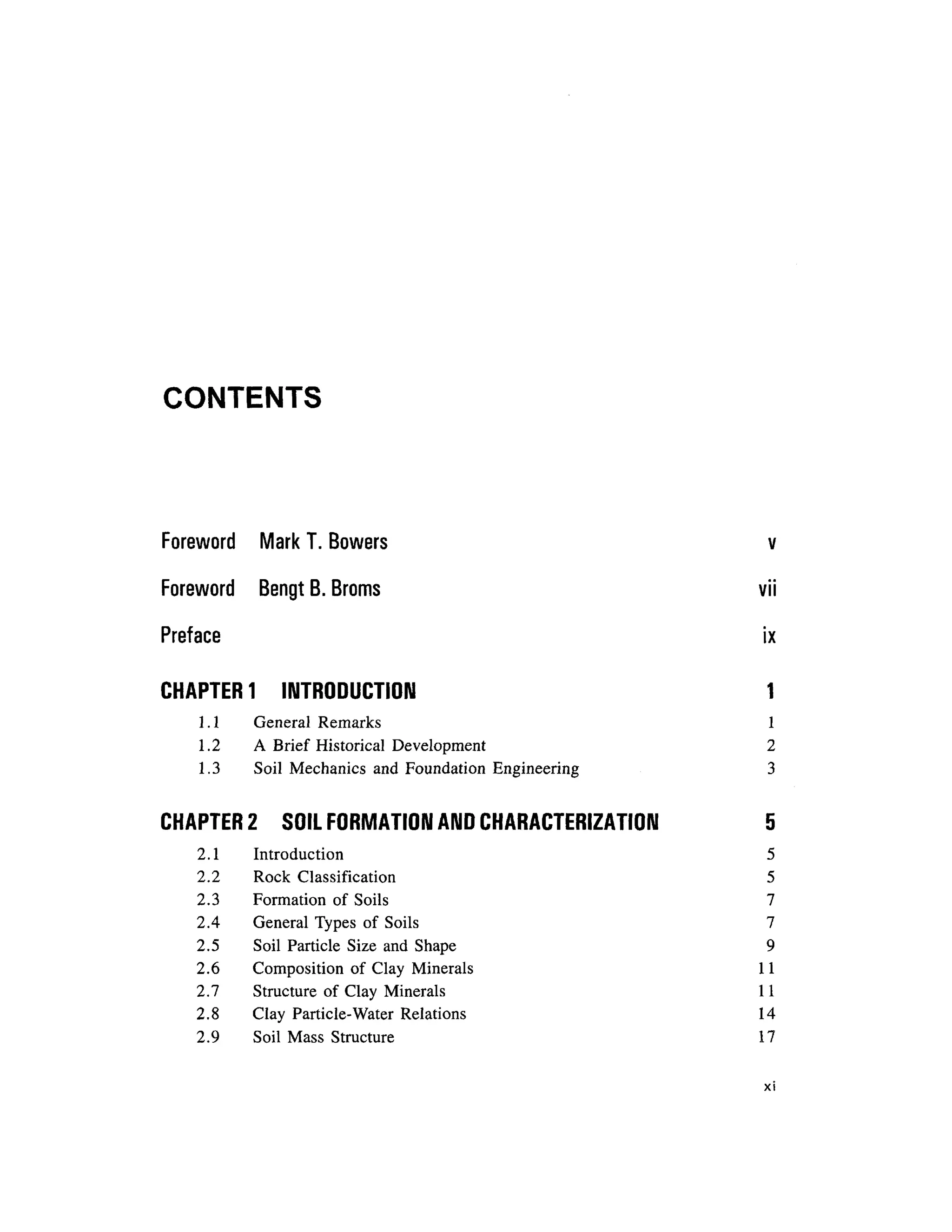
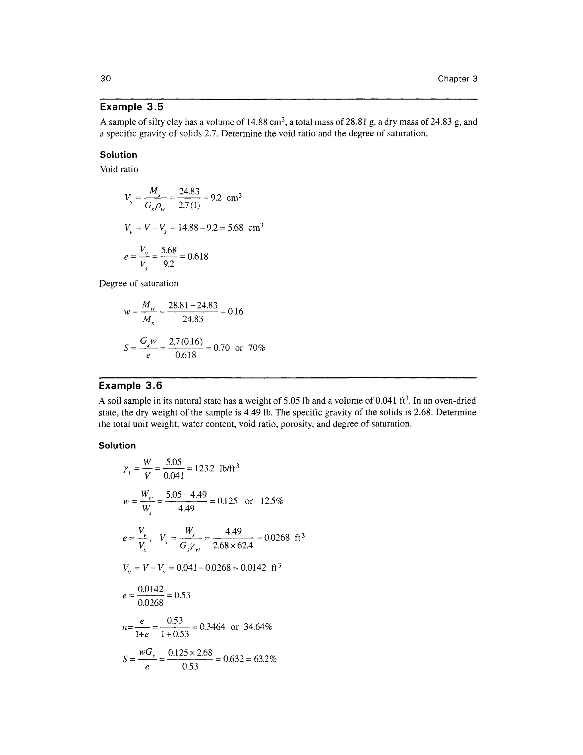
Table 3. 7 Correctio n factor s C fo r uni t weight o f solid s
Gs of soi l solids
2.85
2.80
2.75
2.70
Correction factor C
0.96
0.97
0.98
0.99
Gs of soi l solids
2.65
2.60
2.55
2.50
Correction factor C
1.00
1.01
1.02
1.04

62. Soil Phas e Relationships , Inde x Propertie s an d Soil Classification 4 3
8. Th e hydromete r reading s ar e take n a t th e to p leve l o f th e meniscu s i n bot h th e
sedimentation and control jars.
9. Step s 6 through 8 are repeated by taking hydrometer and temperature readings at elapsed
times of 4, 8, 16, 30, 60 min. and 2, 4, 8, 16, 32, 64 and 96 hr.
10. Necessar y computation s ca n b e mad e wit h th e dat a collecte d t o obtai n th e grain -
distribution curve.
3.9 GRAI N SIZ E DISTRIBUTIO N CURVE S
A typical set of grain size distribution curves is given in Fig. 3.7 with the grain size D as the absciss a
on the logarithmic scale and the percent finer P as the ordinate on the arithmetic scale. On the curve C{
the section AB represents the portion obtained by sieve analysis and the section B'C' by hydrometer
analysis. Since the hydrometer analysis gives equivalent diameters which are generally less than the
actual sizes, the section B'C' will not be a continuation of AB and would occupy a position shown by
the dotted curve. If we assume that the curve BC is the actual curve obtained by sketching it parallel to
B'C', then at any percentage finer, say 20 per cent, the diameters Da and De represent the actual and
equivalent diameters respectively. The ratio of Da to Dg can be quite high for flaky grains.
The shapes of the curves indicate the nature of the soil tested. On the basis of the shapes we
can classify soils as:
1 .Uniforml y graded or poorly graded.
2. Wel l graded.
3. Ga p graded.
Uniformly grade d soil s ar e represente d b y nearl y vertical lines a s show n by curv e C 2 in
Fig. 3.7. Such soils possess particles of almost the same diameter. A well graded soil, represente d
by curve Cp possesses a wide range of particle sizes ranging from grave l to clay size particles. A
gap graded soil, as shown by curve C3 has some of the sizes of particles missing. On this curve the
soil particles falling within the range of XY are missing.
The grain distribution curves as shown in Fig. 3.7 can be used to understand certain grain size
characteristics of soils. Hazen (1893) has shown that the permeability of clean filter sands in a loose
state can be correlated with numerical values designated D10, the effective grain size. The effective
grain size corresponds to 10 per cent finer particles. Haze n found tha t the sizes smaller than the
effective size affected the functioning of filters more than did the remaining 90 per cent of the sizes.
To determine whether a material is uniformly graded or well graded, Hazen proposed the following
equation:
_D
60
where D60 is the diameter of the particle at 60 per cent finer on the grain size distribution curve. The
uniformity coefficient, C u, is about one if the grain size distribution curve is almost vertical, and the
value increases with gradation. For all practical purposes we can consider the following values for
granular soils.
Cu > 4 fo r well graded gravel
Cu > 6 fo r well graded sand
C < 4fo r uniformly graded soil containing particles of the same size

63. 44 Chapter 3
Particle diameter, mm
Figure 3.7 Grai n size distribution curve s
There is another step in the procedure to determine the gradation of particles. This is based on
the term called the coefficient o f curvature whic h is expressed a s
C =
X D
60
(3.35)
wherein D30 is the size of particle at 30 percent finer on the gradation curve. The soil is said to be
well graded i f Cc lies between 1 and 3 for gravels and sands.
Two samples of soils are said to be similarly graded if their grain size distribution curves are
almost parallel to each other on a semilogarithmic plot. Whe n the curves are almost parallel to each
other th e ratio s o f thei r diameter s a t any percentage fine r approximatel y remai n constant . Such
curves are useful i n the design of filter materials around drainage pipes.
3.10 RELATIV E DENSITY O F COHESIONLESS SOILS
The densit y o f granula r soil s varie s wit h th e shap e an d siz e o f grains , th e gradatio n an d th e
manner in which the mass is compacted. I f all the grains are assumed t o be spheres of uniform
size an d packe d a s shown i n Fig. 3.8(a) , the voi d rati o o f such a mass amount s t o about 0.90 .
However, if the grains are packed as shown in Fig. 3.8(b) , the void ratio of the mass is about 0.35 .
The soil corresponding to the higher void ratio is called loose and that corresponding t o the lower
void ratio is called dense. I f the soil grains are not uniform, the n smaller grain s fill i n the spac e
between th e bigge r one s an d th e voi d ratios of suc h soil s ar e reduced t o as low as 0.25 i n th e
densest state . If the grains are angular , they tend t o form looser structure s than rounded grain s

64. Soil Phas e Relationships , Inde x Propertie s an d Soil Classification 4 5
(a) Loosest state (b ) Densest state
Figure 3.8 Packin g of grain s of unifor m size
Table 3.8 Classificatio n o f sand y soil s
Relative density , D f, %
0-15
15-50
50-70
70-85
85-100
Type o f soi l
Very loose
Loose
Medium dens e
Dense
Very dense
because their sharp edges and points hold the grains further apart. If the mass with angular grains
is compacted by vibration, it forms a dense structure. Static load alone will not alter the density
of grains significantly but if it is accompanied by vibration, there will be considerable change in
the density. The water present in voids may act as a lubricant to a certain extent for an increase in
the density under vibration. The change in void ratio would change the density and this in turn
changes the strength characteristics of granular soils. Void ratio or the unit weight of soil can be
used to compare th e strength characteristics of samples of granular soils of the same origin. The
term use d t o indicate the strengt h characteristics i n a qualitative manner is termed a s relative
density which is already expressed by Eq. (3.20). On the basis of relative density, we can classify
sandy soils as loose, medium or dense as in Table 3.8 .
3.11 CONSISTENC Y O F CLAY SOIL
Consistency is a term used to indicate the degree of firmness of cohesive soils. The consistency of
natural cohesive soil deposits is expressed qualitatively by such terms as very soft, soft,stiff , ver y
stiff and hard. The physica l propertie s of clays greatl y diffe r at different water contents. A soi l
which is very soft a t a higher percentage o f water content becomes ver y hard with a decrease in
water content. However, it has been found that at the same water content, two samples o f clay of
different origins may possess different consistency. One clay may be relatively soft while the other
may be hard. Further, a decrease i n water content may have little effect o n one sample of clay but
may transform the other sample from almost a liquid to a very firm condition. Water content alone,
therefore, i s no t a n adequat e inde x o f consistenc y fo r engineerin g an d man y othe r purposes .
Consistency of a soil can be expressed in terms of:
1. Atterber g limits of soils
2. Unconfme d compressive strengths of soils.

65. 46 Chapte r 3
Atterberg Limit s
Atterberg, a Swedish scientist, considered the consistency of soils in 1911, and proposed a series
of tests for defining the properties o f cohesive soils. These test s indicate the range of the plastic
state (plasticity is defined as the property of cohesive soil s which possess the ability to undergo
changes of shape without rupture) and other states. He showed that if the water content of a thick
suspension of clay is gradually reduced, the clay water mixture undergoes changes from a liquid
state throug h a plastic stat e and finally int o a solid state . The different states throug h which the
soil sampl e passe s wit h the decrease i n the moisture content are depicted i n Fig. 3.9 . The water
contents corresponding to the transition from one state to another are termed as Atterberg Limits
and the tests required to determine the limits are the Atterberg Limit Tests. The testing procedures
of Atterberg were subsequently improved by A. Casagrande (1932) .
The transition state from the liquid state to a plastic state is called the liquid limit, wr A t this
stage al l soil s posses s a certai n smal l shea r strength . This arbitraril y chose n shea r strengt h is
probably the smallest value that is feasible to measure in a standardized procedure. Th e transition
from the plastic state to the semisolid state is termed the plastic limit, w . At this state the soil rolled
into threads o f about 3 mm diameter just crumbles. Further decrease of the water contents o f the
same will lead finally to the point where the sample can decrease in volume no further. At this point
the sample begin s to dry a t the surface, saturation is no longer complete , an d further decrease in
water in the voids occurs without change in the void volume. The color of the soil begins to change
from dar k to light. This water content is called the shrinkage limit, ws. The limits expressed above
are all expressed b y their percentages o f water contents. The range o f water content between the
liquid and plastic limits, which is an important measure of plastic behavior, is called the plasticity
index, I } , i.e.,
I
P
= w
rw
p ( 3
-36
)
Figure 3.1 0 depict s th e change s i n volum e fro m th e liqui d limi t t o th e shrinkag e limi t
graphically. The soi l remain s saturate d down t o the shrinkag e limi t and whe n onc e thi s limit is
crossed, the soil becomes partiall y saturated. The air takes the place of the moisture that is lost due
to evaporation. At about 105 ° to 110°C, there will not be any normal water left in the pores and soil
at thi s temperatur e i s sai d t o be oven-dry. A soi l sampl e o f volum e V o and wate r conten t wo is
represented b y point A in the figure .
As th e soi l lose s moisture content there i s a corresponding chang e i n the volum e of soils .
The volum e chang e o f soi l i s equa l t o th e volum e o f moistur e lost . Th e straigh t line , AE ,
therefore, give s th e volum e of th e soi l a t different wate r contents. Points C and D represen t th e
transition stages o f soil sampl e at liquid and plastic limits respectively. As the moisture content is
reduced furthe r beyon d the point D, the decrease i n volume of the soil sampl e wil l not be linear
States
Liquid
w,
Plastic
wn
p
Semi solid
. .. . w
Solid
Limit
Liquid limit
Plastic limit
Shrinkage limit . .
Consistency
Very sof t
Soft
Stiff
.. Ver y stif f
Extremely stif f
Hard
Volume change
!
Decrease in volume
i
Constant volume
Figure 3.9 Differen t state s an d consistency o f soils with Atterberg limits

66. Soil Phas e Relationships , Inde x Propertie s and Soil Classification 47
(V0-VS) 2
SolidI Semi-soli d^
state stat e Plastic state
Liquid
~ stat e
A
Vs
= Volum e of solids
Va
= Volum e of air
Vd
= Volum e of dry soil
Vw
= Volum e of water
Water content
Figure 3.10 Curv e showin g transition stages fro m the liquid to soli d state
with the decrease in moisture beyond a point E due to many causes. One possible caus e is that air
might star t enterin g int o th e void s o f th e soil . Thi s ca n happe n onl y whe n th e norma l wate r
between the particles i s removed. If the normal water between some particles i s removed, the soil
particles surrounde d by absorbed wate r will come in contact wit h each other . Greater pressur e is
required i f these particles are to be brought still closer. As such the change in volume is less than
the chang e i n moistur e content . Therefore, th e curve DEBT depict s th e transitio n fro m plasti c
limit to the dry condition of soil represented b y point F. However, for all practical purposes , th e
abscissa o f the point of intersection B of the tangents FB and EB ma y be taken a s the shrinkag e
limit, ws. The straight line AB whe n extended meet s the ordinate a t point M. The ordinat e o f M
gives th e volum e of the soli d particle s V, . Sinc e th e ordinat e o f F is the dr y volume , V d, of th e
sample, th e volume of air V fl, is given by (Vd- V s}.
3.12 DETERMINATIO N O F ATTERBERG LIMIT S
Liquid Limi t
The apparatu s shown in Fig. 3.11 is the Casagrande Liquid Limit Device use d for determining th e
liquid limits of soils. Figure 3.12 shows a hand-operated liquid limit device. The device contains a
brass cup which can be raised and allowed to fall on a hard rubber base by turning the handle. The cup
is raised by one cm. The limits are determined on that portion of soil finer than a No. 40 sieve (ASTM
Test Designation D-4318). About 100 g of soil is mixed thoroughly with distilled water into a uniform
paste. A portion o f the past e i s placed i n the cu p an d leveled t o a maximum dept h o f 1 0 mm. A
channel o f th e dimension s of 1 1 m m widt h and 8 mm dept h i s cut throug h th e sampl e alon g th e

67. 48 Chapter 3
Brass cup
Sample ^ ,
Liquid limit device
Hard stee l
Casagrandes groovin g tool AST M grooving tool
Figure 3.11 Casagrande' s liquid limit apparatu s
symmetrical axi s of the cup. The grooving tool should always be held normal to the cup at the point of
contact. The handle is turned at a rate of about two revolutions per second an d the number of blows
necessary t o close th e groove alon g th e bottom fo r a distance of 12. 5 mm i s counted. Th e groov e
should be closed b y a flow o f the soil and not by slippage between the soil an d the cup. The water
content of the soil in the cup is altered an d the tests repeated. At least four tests should be carried ou t
by adjusting th e water contents in such a way that the number of blows required t o close the groov e
may fall within the range of 5 to 40. A plot of water content against the log of blows is made as shown
in Fig. 3.13. Within the range of 5 to 40 blows, the plotted point s li e almost o n a straight line . The
curve so obtained is known as a 'flow curve'. The water content corresponding t o 25 blows i s termed
the liquid limit. The equation of the flow curv e can be written as
= -I fogN+C (3.37)
where, w = wate r content
/,= slop e of the flow curve , termed a s flow index
N= numbe r of blows
C= a constant.
Liquid Limi t b y One-Poin t Metho d
The determination of liquid limi t as explained earlier require s a considerable amoun t of time and
labor. W e can us e wha t is termed th e 'one-poin t method ' if an approximate valu e of th e limi t is
required. The formula used for this purpose is
(N
(3.38)

68. Soil Phas e Relationships , Inde x Propertie s an d Soil Classificatio n 4 9
Figure 3.12 Hand-operate d liquid limit device (Courtesy: Soiltest, USA )
where w is the water content corresponding to the number of blows N, and n, an index whose value has
been foun d t o var y from 0.06 8 t o 0.121 . An averag e valu e of 0.104 ma y b e usefu l fo r al l practica l
purposes. It is, however, a good practice to check this method with the conventional method as and when
possible.
Liquid Limi t by the Us e o f Fal l Con e Penetromete r
Figure 3.1 4 show s th e arrangemen t o f th e apparatus . Th e soi l whos e liqui d limi t i s t o b e
determined i s mixed wel l int o a soft consistenc y an d pressed int o the cylindrical mol d o f 5 cm
diameter an d 5 cm high. The cone which has a central angle of 31° and a total mass of 14 8 g will
be kept free on the surfac e of the soil. The depth of penetration3; of the cone is measured i n mm
on the graduated scale afte r 3 0 sec of penetration. The liquid limit wl may be computed by using
the formula,
Wf = wy + 0.01(25 - y)(wy + 15) (3.39 )
where w i s the water content corresponding to the penetration y .
The procedure i s based o n the assumption that the penetration lies between 20 and 30 mm.
Even this method has to be used with caution.
Plastic Limi t
About 1 5 g of soil, passing through a No. 40 sieve, is mixed thoroughly . The soi l i s rolled o n a
glass plate with the hand, until it is about 3 mm in diameter. This procedure of mixing and rolling
is repeated til l the soil shows signs of crumbling. The water content of the crumbled portion of the
thread is determined. This is called the plastic limit.

69. 50 Chapter 3
ON
o
^
co
4^
o
o
s
NJ
o
Liquid limit
C
3 4 6 8 1 0 2 0 2 5
Log number of blows N
40 6 0 100
Figure 3.13 Determinatio n o f liquid limit
Shrinkage Limi t
The shrinkage limit of a soil can be determined by either of the following methods :
1. Determinatio n of vv s, when the specific gravity of the solids Gs is unknown.
2. Determinatio n of vv v, when the specific gravity of the solids, G s is known.
Figure 3.14 Liqui d limit b y the us e of th e fal l con e penetrometer : (a ) a schemati c
diagram, an d (b ) a photograph (Courtesy : Soiltest , USA)

70. Soil Phas e Relationships , Inde x Propertie s and Soil Classification 51
Method I When G f i s Unknown
5
Three block diagrams of a sample of soil having the same mass of solids Ms, are given in Fig. 3.15.
Block diagram (a) represents a specimen in the plastic state, which just fills a container of known
volume, Vo. The mass of the specimen is Mo. The specimen is then dried gradually, and as it reaches
the shrinkag e limit , the specime n i s represente d b y bloc k diagra m (b) . The specime n remain s
saturated up to this limit but reaches a constant volume Vd. When the specimen is completely dried,
its mass will be Ms wherea s its volume remains as Vd.
These different state s are represented in Fig. 3.10. The shrinkage limit can be written as
M
w =
M,
where, M = M
(3.40)
Ms- (V o - V d) pw
Therefore w =
M
x 100% (3.41)
The volume of the dry specimen can be determined either by the displacement o f mercury
method or wax method. Many prefer the wax method because wax is non-toxic. The wax method is
particularly recommended i n an academic environment.
Determination o f Dr y Volum e V d of Sampl e b y Displacemen t i n Mercury
Place a small dish filled with mercury up to the top in a big dish. Cover the dish with a glass plate
containing three metal prongs in such a way that the plate is entrapped. Remove the mercury spilt
over into the big dish and take out the cover plate from th e small dish. Place the soil sampl e on
the mercury. Submerge th e sample with the pronged glass plate and make th e glass plate flus h
with the top of the dish. Weigh the mercury that is spilt over due to displacement. The volume of
the sample is obtained by dividing the weight of the mercury by its specific gravity which may be
taken as 13.6 . Figure 3.16 shows the apparatus used for the determination of dry volume.
Method I I When G 0 is Known
o
M
100 where, M w = (V d-Vs)pw =
M
T
M
(a) (b ) (c )
Figure 3.15 Determinatio n of shrinkag e limit

71. 52 Chapter 3
Glass plate
Figure 3.16 Determinatio n o f dry volume by mercury displacemen t metho d
Therefore, v v= •
M
-xlOO = xlOO (3.42)
or w = -^ --
- -xlO O (3.43)
where, p = 1 for all practical purposes .
3.13 DISCUSSIO N ON LIMITS AN D INDICES
Plasticity index and liquid limit are the important factors that help an engineer to understand the
consistency o r plasticit y of a clay. Shearing strength , though constant a t liqui d limits , varie s a t
plastic limits for all clays. A highly plastic clay (sometimes calle d a fat clay) has higher shearin g
strength at the plastic limit and the threads at this limit are rather hard to roll whereas a lean clay can
be rolled easily at the plastic limit and thereby possesses lo w shearing strength.
There are some fin e graine d soils that appear simila r to clays but they cannot be rolled into
threads so easily. Such materials are not really plastic. They may be just at the border line between
plastic and non-plastic soils. In such soils, one finds th e liquid limit practically identical with the
plastic limit and 1=0.
Two soils may differ i n their physical properties eve n though they have the same liqui d and
plastic limits or the same plasticity index. Such soils possess different flow indices. For example in
Fig. 3.17 are shown two flow curves C, and C2 of two samples of soils. C } is flatter than C2. It may
be assume d fo r th e sak e o f explanatio n that bot h th e curve s ar e straigh t line s eve n whe n th e
moisture content in the soil is nearer the plastic limit and that the same liquid limit device is used to
determine th e numbe r o f blow s require d t o clos e th e groov e a t lowe r moistur e contents . Th e
plasticity index / i s taken to be the same for both the soils. It can be seen fro m the figure that the
sample o f flo w curve C , has liqui d and plastic limit s of 10 0 and 8 0 percent respectively , givin g
thereby a plasticity index / o f 20 per cent. The sample of flow curve C2 has liquid and plastic limits
of 5 4 an d 3 4 percent givin g thereb y th e sam e plasticit y index valu e of 2 0 percent . Thoug h th e
plasticity indice s of the two samples remai n the same, th e resistance offere d b y the two sample s
for slippage at their plastic limits is different. Sampl e one takes 90 blows for slippage whereas th e
second on e takes only 40 blows. This indicates that at the plastic limits, the cohesive strengt h of
sample 1 with a lower flow inde x is larger than that of sample 2 with a higher flow index .

72. Soil Phas e Relationships, Inde x Propertie s an d Soil Classificatio n 53
4 6 1 0 2 0 2 5 4 0 6 0 10 0
Log number of blows N
Figure 3.17 Tw o sample s of soils with different flo w indice s
Plasticity Inde x lp
Plasticity index / indicate s th e degree o f plasticity of a soil. The greater th e difference betwee n
liquid an d plasti c limits , th e greate r i s th e plasticit y o f th e soil . A cohesionles s soi l ha s zer o
plasticity index. Such soils are termed non-plastic. Fat clays are highly plastic and possess a high
plasticity index. Soils possessing larg e values of w, and / ar e said to be highly plastic or fat. Those
with low values are described a s slightly plastic or lean. Atterberg classifies the soils according to
their plasticity indices as in Table 3.9 .
A liqui d limit greate r tha n 10 0 is uncommo n fo r inorgani c clay s o f non-volcani c origin .
However, fo r clay s containin g considerabl e quantitie s o f organi c matte r an d clay s o f volcani c
origin, the liquid limit may considerably exceed 100 . Bentonite, a material consisting of chemically
disintegrated volcanic ash, has a liquid limit ranging from 400 to 600. It contains approximately 70
percent o f scale-like particle s o f colloidal siz e a s compared wit h abou t 30 per cen t for ordinary
highly plastic clays. Kaolin and mica powder consist partially or entirely of scale like particles of
relatively coars e siz e i n compariso n wit h highl y colloida l particle s i n plasti c clays . The y
therefore posses s les s plasticit y than ordinary clays. Organic clay s posses s liqui d limit s greate r
than 50. The plastic limit s of such soils are equally higher. Therefore soil s wit h organic content
have low plasticity indices correspondin g t o comparatively high liquid limits.
Table 3.9 Soi l classification s accordin g t o Plasticit y Inde x
Plasticity index Plasticity
0
<7
7-17
Non-plastic
Low plastic
Medium plastic
Highly plastic

73. 54 Chapte r 3
Toughness Index , lt
The shearing strength of a clay at the plastic limit is a measure of its toughness. Two clays having
the same plasticity index possess toughness which is inversely proportional t o the flow indices. An
approximate numerical valu e for the toughness can be derived as follows.
Let s l = shearin g strength corresponding t o the liquid limit, wf, whic h is assumed t o be
constant for all plastic clays.
s = shearin g strengt h a t th e plasti c limit , whic h ca n b e use d a s a measur e o f
toughness of a clay.
NowWj = -lf logAf , + C, w p = -If logN p + C
where N( an d N ar e the number of blows at the liquid and plastic limits respectively. The flow curve
is assumed to be a straight line extending into the plastic range as shown in Fig. 3.17.
Let, N{ = msr N } = ms , wher e m is a constant.
We can write
wl = -I,ogms[ + C,w - -I,ogms + C
Therefore l
p = w
i~w
p = If(logmsp-ogmSl)=I fog-?-
si
or t
=
T
= g
~ ( 3
-44
>
Since w e ar e interested onl y in a relative measur e o f toughness , l t can b e obtaine d fro m
Eq. (3.44) a s the ratio o f plasticity index an d flo w index . The valu e of I ( generall y fall s betwee n
0 and 3 for most clay soils. When It is less than one, the soil is friable at the plastic limit. It is quite
a useful inde x to distinguish soils of different physica l properties .
Liquidity Inde x /,
The Atterberg limits are found for remolded soi l samples. These limits as such do not indicate
the consistenc y o f undisturbe d soils . Th e inde x tha t i s use d t o indicat e th e consistenc y o f
undisturbed soils is called the liquidity index. The liquidity index is expressed a s
7
/=^—~ (3.45 )
where, wn is the natural moisture content of the soil in the undisturbed state. The liquidity index of
undisturbed soil can vary from les s than zero to greater tha n 1. The value of I { varie s according t o
the consistency o f the soil as in Table 3.10.
The liquidity index indicates the state of the soil in the field. If the natural moisture content of
the soil is closer to the liquid limit the soil can be considered a s soft, and the soil is stiff if the natural
moisture content is closer to the plastic limit. There are some soils whose natural moisture content s
are higher tha n th e liqui d limits . Such soil s generall y belon g t o the montmorillonit e grou p an d
possess a brittle structure. A soil of this type when disturbed by vibration flows like a liquid. The
liquidity inde x value s o f such soil s ar e greater tha n unity. One has t o be cautious in using such
soils fo r foundations of structures.

74. Soil Phase Relationships , Inde x Propertie s and Soil Classification 5 5
Table 3.10 Value s of / / and lc according to consistenc y o f soi l
Consistency / / l c
Semisolid or solid stat e Negativ e > 1
Very stiff stat e (wn = wp) 0 1
Very soft state (w n = wl) 1 0
Liquid stat e (whe n disturbed) > 1 Negativ e
Consistency Index , /C
The consistency index may be defined as
/ (3.46 )
p
The index lc reflects the state of the clay soil condition in the field in an undisturbed state just in the
same way as It describe d earlier . The values of / fo r different state s of consistency ar e given in
Table 3.10 along with the values Ir I t may be seen that values of 7, and Ic are opposite to each other
for the same consistency of soil.
From Eqs (3.45) and (3.46) we have
wl — w
I
i+I
c= j P
= l
(3.47 )
p
Effect o f Dryin g o n Plasticity
Drying produces an invariable change in the colloidal characteristics of the organic matter in a soil.
The distinction between organi c and inorganic soils can be made by performing tw o liquid limit
tests on the same material. On e test is made on an air-dried sample and the other on an oven-drie d
one. If the liquid limit of the oven-dried sample is less than about 0.75 times that for the air-dried
sample, the soils may be classed a s organic. Oven-drying also lowers the plastic limits of organic
soils, but the drop in plastic limit is less than that for the liquid limit.
Shrinking an d Swelling o f Soil s
If a mois t cohesiv e soi l i s subjecte d t o drying , it lose s moistur e an d shrinks . Th e degree o f
shrinkage, S , is expressed a s
. , = - x (3.48a )
o
where,
Vo = original volume of a soil sample at saturated state
Vd = final volume of the sample at shrinkage limit
On the basis of the degree of shrinkage, Scheidig (1934) classified soils as in Table 3.11.
Shrinkage Rati o SR
Shrinkage rati o i s define d a s th e rati o o f a volum e change expresse d a s a percentage o f dry
volume to the corresponding change in water content above the shrinkage limit .

75. 56 Chapte r 3
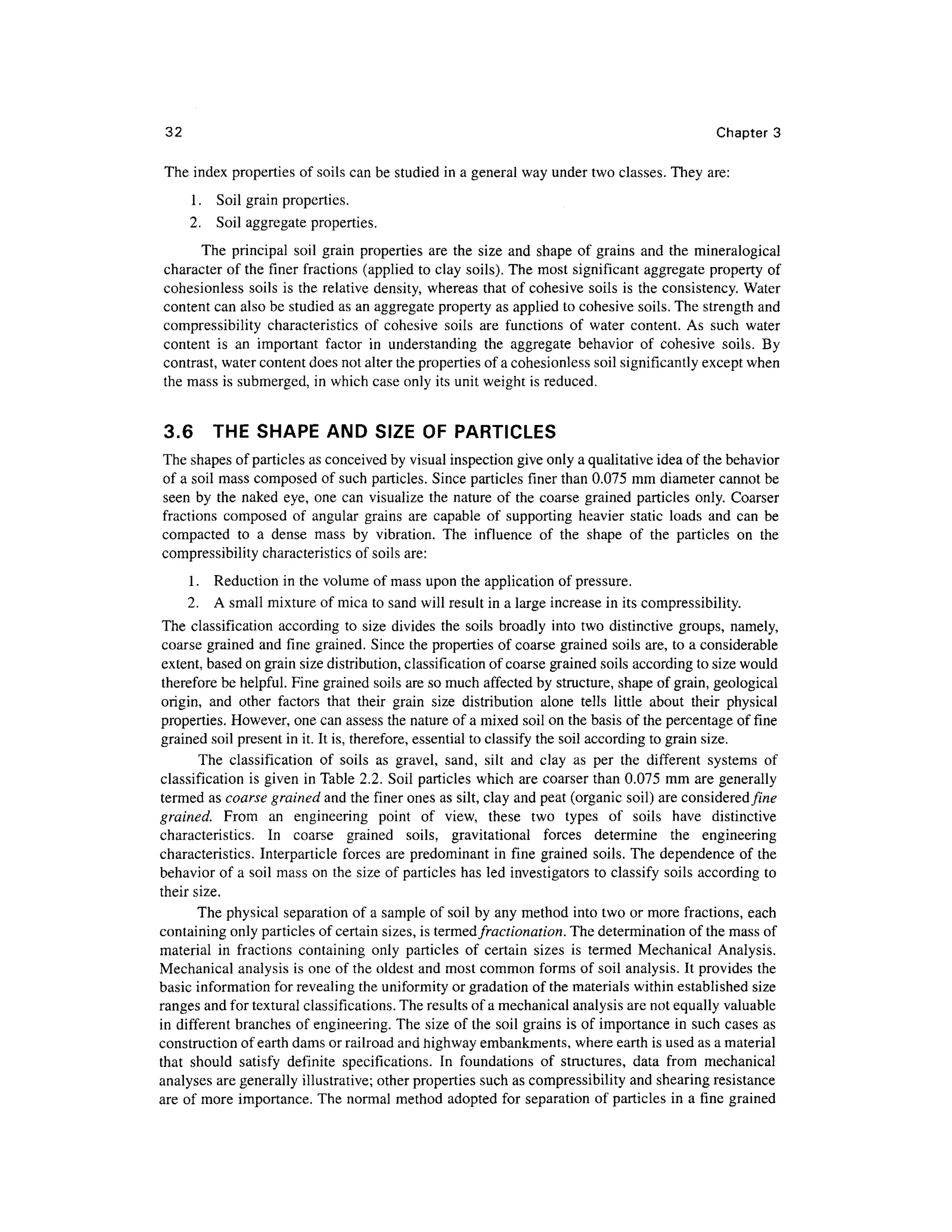
Table 3.11 Soi l classificatio n accordin g t o degre e o f shrinkag e S r
Sr% Qualit y o f soi l
< 5 Goo d
5-10 Mediu m goo d
10-15 Poo r
> 1 5 Ver y poor
(V -V,)/V,
SR=' ° d)l d
xlO O (3-48b )
W
0~W
S
where
Vo = initial volume of a saturated soil sample at water content wo
Vd = the final volume of the soil sample at shrinkage limit ws
(wo-ws) = change in the water content
Md = mass of dry volume, Vd, of the sample
Substituting for (wo-ws) i n Eq (3.48b) and simplifying, we have
• ; - • - •
Thus the shrinkage ratio of a soil mass is equal to the mass specific gravity of the soil in its
dry state .
Volumetric Shrinkag e Sv
The volumetric shrinkage or volumetric change is defined as the decrease i n volume of a soil mass,
expressed as. apercentage of the dry volume of the soil mas s whe n the water conten t is reduce d
from the initial wo to the final w s at the shrinkage limit.
d
(3.49)
Linear shrinkage ca n be computed fro m the volumetric change by the following equatio n
1/3
5.. +1.0
LS= l
~ c 1 m Xl
°° percen t
(3-50 )
The volumetri c shrinkag e Sv i s use d a s a decima l quantit y in Eq . (3.50) . Thi s equatio n
assumes that the reduction in volume is both linear and uniform in all directions.
Linear shrinkage can be directly determined by a test [this test has not yet been standardized
in the United States (Bowles, 1992)]. The British Standard BS 1377 used a half-cylinder of mold of
diameter 12. 5 mm and length Lo = 140 mm. The wet sample filled int o the mold is dried and the
final lengt h L,is obtained. Fro m this , the linear shrinkage LS is computed a s

76. Soil Phase Relationships, Inde x Propertie s an d Soil Classification 57
LS =
L-L.
(3.51)
Activity
Skempton (1953) considers that the significant change in the volume of a clay soil during shrinking
or swelling is a function o f plasticity index and the quantity of colloidal cla y particles presen t in
soil. The clay soil can be classified inactive, normal or active (after Skempton, 1953). The activity
of clay is expressed as
Activity A =
Plasticity index, /
Percent fine r tha n 2 micro n
(3.52)
Table 3.12 gives the typ e of soi l accordin g to the valu e of A. The cla y soi l whic h has an
activity value greater than 1.4 can be considered as belonging to the swelling type. The relationship
between plasticity index and clay fraction i s shown in Fig. 3.18(a).
Figure 3.18(b ) show s result s o f som e test s obtaine d o n prepare d mixture s o f variou s
percentage o f particles les s than and greater than 2 /^. Severa l natura l soils wer e separate d int o
fractions greater and less than 2 /z and then the two fractions were combined as desired. Fig 3.18(c)
shows the results obtained on clay minerals mixed with quartz sand.
Table 3.12 Soi l classification accordin g to activit y
A Soi l type
<0.75 Inactiv e
0.75-1.40 Norma l
>1.40 Activ e
Plasticity
index,
I
p
•—
K
>
U
>
-£>
.
Lf>
O
D
O
O
O
O
O
O
Acti
/
//
VQ soil
/
//
/1
{
s
/
A
Nformal s o
/*
Inactiv
/
11
jr
^/l = (
e soil
•0
.75
10 2 0 3 0 4 0 5 0
Percent finer than 2 micron
60
Figure 3.18(a) Classificatio n of soi l according t o activit y

77. 58 Chapter 3
1UU
80
X
16 0
'o
1 4
0
a,
20
°(
/
»&
y
//
^o>
/y
<*
Shell
y( 1
Lone
((
haven
33)
Ion clay
).95)
Weald clay
^ (0-95 )
Horten
(0.95)
) 2 0 4 0 6 0 8 0 1 G
500
400
300
200
100
mon
f,
/
Sodium
tmorillo
(1.33)
/
/
^ „— — —""
aite
/
/
.---"KaoHnite
T
(A=0.9_)
Clay fraction (< 2//) (%)
(b)
20 4 0 6 0 8 0
Clay fractio n ( < 2//)(%)
(c)
100
Figure 3.18(b, c) Relatio n between plasticit y inde x an d clay fraction. Figure s in
parentheses ar e the activities o f th e clay s (afte r Skempton, 1953 )
Consistency o f Soil s a s per the Unconfine d Compressiv e Strengt h
The consistency of a natural soil is different fro m that of a remolded soil at the same water content.
Remolding destroys the structure of the soil and the particle orientation. The liquidity index value
which is an indirect measure of consistency is only qualitative. The consistency of undisturbed soil
varies quantitativel y on th e basi s o f it s unconfine d compressiv e strength . Th e unconfme d
compressive strength , q u, i s define d a s th e ultimat e loa d pe r uni t cros s sectiona l are a tha t a
cylindrical specimen o f soil (with height to diameter ratio of 2 to 2.5) can take under compressio n
without an y latera l pressure. Water content of the soil i s assumed to remain constant during the
duration of the test which generally takes only a few minutes. Table 3.13 indicates the relationship
between consistency and qu.
As explaine d earlier , remoldin g o f a n undisturbe d sampl e o f cla y a t th e sam e wate r
content alters its consistency, because of the destruction of its original structure. The degree of
disturbance of undisturbed clay sample due to remolding can be expressed a s
Table 3.13 Relationshi p betwee n consistenc y o f clay s an d qu
Consistency
Very sof t
Soft
Medium
qu, kN/m 2
<25
25-50
50-100
Consistency
Stiff
Very stif f
Hard
qu, kN/m 2
100-200
200-400
>400
Table 3.14 Soi l classification on the basis of sensitivity (afte r Skempton an d
Northey, 1954 )
s
t
1
1-2
2-4
Nature of cla y
Insensitive clays
Low-sensitive clay s
Medium sensitiv e clays
S
t
4-8
8-16
Nature o f cla y
Sensitive clays
Extra-sensitive clay s
Quick clay s

78. Soil Phas e Relationships, Index Propertie s an d Soil Classificatio n 59
Sensitivity, S r =
qu, undisturbed
q'u, remolde d (3.53)
where q'u is the unconfmed compressive strength of remolded clay at the same water content as that
of the undisturbed clay.
When q'u is very low as compared to qu the clay is highly sensitive. When qu =q'u the clay is said to
be insensitive to remolding. On the basis of the values of St clays can be classified as in Table 3.14.
The clays that have sensitivit y greater tha n 8 should be treated wit h care durin g constructio n
operations because disturbance tends to transform them, at least temporarily, into viscous fluids. Such
clays belong to the montmorillonite group and possess flocculent structure .
Thixotropy
If a remolded cla y sampl e wit h sensitivity greate r tha n one i s allowe d t o stan d withou t furthe r
disturbance an d chang e i n water content , i t may regain a t least par t o f its origina l strengt h an d
stiffness. This increase in strength is due to the gradual reorientation o f the absorbed molecule s of
water, and is known as thixotropy (fro m the Greek thix, meaning 'touch' and tropein, meaning 'to
change'). Th e regainin g o f a part o f th e strengt h afte r remoldin g ha s importan t application s i n
connection wit h pile-driving operations , an d other type s of construction i n which disturbance of
natural clay formations is inevitable.
3.14 PLASTICIT Y CHAR T
Many properties of clays and silts such as their dry strength, compressibility an d their consistenc y
near the plastic limit can be related with the Atterberg limits by means of a plasticitychart as shown
is Fig . 3.19 . I n thi s char t th e ordinate s represen t th e plasticit y inde x 7 an d th e abscissa s th e
40 6 0
Liquid limit, w,
Figure 3.19 Plasticit y char t
80 100

79. 60 Chapte r 3
corresponding liqui d limit wr The chart is divided into six regions, three above and three below line
A, The equation to the line A is
7p = 0.73 (W/- 20) (3.51 )
If a soil is known to be inorganic its group affiliation ca n be ascertained o n the basis of the
values of/ an d wl alone. However, points representing organic clays are usually located withi n the
same regio n a s those representing inorganic silts of high compressibility, an d points representin g
organic silt s in the region assigne d to inorganic silts of medium compressibility .
Casagrande (1932) studied the consistency limits of a number of soil and proposed the plasticity
chart shown in Fig. 3.19. The distribution of soils according to the regions are given below .
Region
Above /4-line
1
2
3
Below /4-line
4
5
6
Liquid limi t w t
Less than 30
30 < W j < 5 0
w,>50
wl<30
30<w,< 50
w,>50
Type o f soi l
Inorganic clays of low plasticity and cohesionless soil s
Inorganic clay s of medium plasticity
Inorganic clays of high plasticity
Inorganic silts of low compressibility
Inorganic silts of medium compressibility and organic silts
Inorganic silts of high compressibility an d organic cla y
The uppe r limit of the relationship between plasticit y index and liquid limit is provided b y
another line called the [/-line whose equation is
I = 0.9(w-&)(3.52 )
Example 3. 9
Determine th e times (? ) required for particles o f diameters 0.2 , 0.02 , 0.0 1 an d 0.005 mm to fall a
depth of 1 0 cm from the surface in water.
Given:JL = 8.15 x 10~ 3
poises, G = 2.65. (Note : 1 poise = 10~ 3
gm-sec/cm2
)
Solution
H = 8.15 x 10~ 3
x 10~ 3
= 8.15 x lO^ 6
gm-sec/cm2
.
Use Eq. (3.24)
30// L 30X8.15X10" 6
1 0 1.48 2 x!0~3
.
- x — -= -
- -
m m
(Gs-l) D 2
(2.65-1 ) D 2
D 2
The times required fo r the various values of D are as given below.
D (mm) t
0.2
0.02
0.01
0.005
2.22 sec
3.71 mi n
14.82 mi n
59.28 min

80. Soil Phas e Relationships , Inde x Propertie s an d Soil Classification 6 1
Example 3.1 0
A sedimentation analysis by the hydrometer method (152 H) was conducted wit h 50 g (= A/s)of
oven dried soil. The volume of soil suspension is V =103
cm3
. The hydrometer reading Ra = 19.50
after a lapse of 60 minutes after the commencement of the test.
Given: Cm (meniscus) = 0.52, L (effective) = 14.0 cm, Co (zero correction) = +2.50, Gs =2.70
and [i = 0.01 poise .
Calculate the smallest particl e size , whic h woul d have settled a depth o f 14. 0 c m and the
percentage finer than this size. Temperature of test = 25° C.
Solution
From Eq. (3.24)
D(mm) =
where ^ = 0.01 x 10~ 3
(gm-sec)/cm2
.
Substituting
SOxO.OlxlO-3
1 4
£>- -
XJ — = 0.0064 mm .
V (2.7-1 ) V6 0
From Eq. (3.31)
From Table 3.6 for T= 25 °C, Cr=+1.3. Therefore ,
Rc =19.5-2.5 +1.3=18.3
From Eqs (3.32) and (3.31), we have
CR 1.65G .
, C =
Ms
sg
2.65(G-1 )
= 1.65X2. 7 p .%
sg
2.65(2.7-1 ) 5 0
Example 3.1 1
A 500 g sample of dry soil was used for a combined siev e and hydrometer analysis (152 H type
hydrometer). Th e soi l mas s passin g throug h the 7 5 fi siev e = 12 0 g. Hydrometer analysi s wa s
carried out on a mass of 40 g that passed through the 75(Ji sieve. The average temperature recorde d
during the test was 30°C.
Given: Gs =2.55, C m (meniscus) = 0.50, C o =+2.5, n =8.15 x 10~ 3
poises.
The actual hydrometer reading Ra = 15.00 after a lapse of 120 min after the start of the test.
Determine the particle size D and percent finer P'% and P%.
Solution
From Eq. (3.29 )
L =16.3-0.16417?

81. 62
where, R = Ra + Cm = 15.0 + 0.5 = 15. 5
L = 16.3 -0.1641 x15.5 =13.757
From Eq. (3.24 )
Chapter 3
30x8.15xlO-6
13.75 7 ^ 0
x.|
= 0.004 3 m
m
2.55-1
From Eq . (3.32 )
C R
Percent finer , P'% = S8 c
x 100
M
From Table 3.7, C = 1.02 for Gs =2.55
From Table 3.6, Cr = +3.8 for T= 30 °C
Now, R c = R
a- Co + CT = 15 - 2.5 + 3.8 = 16. 3
Now, /"= L 0 2 x l 6 3
x 100 = 41.57%
P% = 41.57 x
40
—
500
Example 3.1 2
500 g of dry soil was used for a sieve analysis. The masses of soil retained on each sieve are given below:
US standard sieve
2.00 mm
1 .4
0 mm
1.00mm
Mass i n g
10
18
60
US standard sieve
500 fj.
250 j U
125/1
75 fji
Mass in
135
145
56
45
g
Plot a grain size distribution curve and compute the following:
(a) Percentages o f gravel, coarse sand , medium sand, fine sand and silt, as per the Unified
Soil Classification System, (b) uniformity coefficient (c) coefficient of curvature.
Comment on the type of soil.
Solution
Computation of percen t fine r
US stand- Diameter , D
ard siev e o f grain s i n m m
2.00 mm
1 .4
0 mm
1.00mm
500/1
250 fj,
125/1
75 p.
2.00
1.40
1.00
0.500
0.25
0.125
0.075
Mass
retained in g
10
18
60
135
145
56
45
%
retained
2.0
3.6
12.0
27.0
29.0
11.2
9.0
Cumulative
% retaine d
2.0
5.6
17.6
44.6
73.6
84.8
93.8
%
finer P
98.0
94.4
82.4
55.4
26.4
15.2
6.2

82. Soil Phase Relationships , Inde x Propertie s and Soil Classification 63
100
90
80
70
g 6 0
<5
<| 5 0
<u
£ 4 0
OH
30
20
10
n
Gravel
Sand
Coarse to medium
«
60%
^
V
A*r
1
r
309
£>3o
Fine
>,
N,
A
10%
D ~**
^
(
e
Silt + clay
108 6 4 2 1 .8 .6 . 4 0. 2 0.1.08.06.0 4 .0 2
Grain diameter, D in mm
Figure Ex. 3.12
(a) Percentage coars e to medium sand = 98 - 4 8 = 50 percent
Percentage fin e sand = 48 - 6. 2 =41.8 percent
Percentage sil t and clay = 6.2 percent.
ZXn
(b) Uniformity coefficient C =
DIQ 0.09 8
(c) Coefficient of curvature C =
= 5.92
(0.28)2
iyxD60 0.098x0.5 8
The soil is just on the border line of well graded sand .
= 1.38
Example 3.1 3
Liquid limit tests on a given sample of clay were carried out. The data obtained are as given below.
Test No. 1
Water content, % 7 0
Number of blows, N 5
64 47
30
44
45
Draw the flow curve on semi-log paper and determine the liquid limit and flow index of the soil.
Solution
Figure Ex. 3.1 3 give s the flow curv e for the given sample of clay soil. As per the curve,
Liquid limit, v{ = 50%
Flow index , /, =29

83. 64 Chapter 3
70
60
S3 5 0
I
40
30
No
2 4 6 81 0 202 5 4 0 608010 0
Number o f blows
Figure Ex. 3.13
Example 3.14
The laborator y test s on a sample of soil gave the following results:
wn - 24% , w, = 62%, wp = 28%, percentage of particles less than 2 JJL - 23%
Determine: (a ) The liquidit y index, (b) activity (c ) consistency and nature of soil .
Solution
(a) Plasticit y index, Ip = wl- wp = 62 - 2 8 = 34%
wn -w 24-2 8
Liquidity index , 7 , = —p
- = — = -0.12.
(b) Activity , A -
34
p
*P
= 34
of particles < 2/u 2 3
= 1.48.
(c) Comments :
(i) Since I : is negative, the consistency of the soil is very stiff to extremely stiff
(semisolid state).
(ii) Since I is greater than 17% the soil is highly plastic.
(Hi) Since A is greater than 1.40, thesoil is active and is subject to significant volume
change (shrinkage and swelling).
Example 3.15
Two soil sample s teste d i n a soil mechanics laboratory gave the following results:
Sample no . 1 Sampl e no. 2
Liquid limi t 50 %
Plastic limi t 30 %
Flow indices , /, 2 7
40%
20%
17

84. Soil Phase Relationships, Inde x Propertie s and Soil Classification 6 5
(a) Determine the toughness indices and
(b) comment on the types of soils.
Solution
w, - w
S~ 7 _ ' P
Sample ,, ,, = Z . =
= 0.74 ; Sampl e 2, /, = . =
= 1.18
F
' 2 7 2 7 1 7 1 7
(b)
(i) Bot h the soils are clay soils as their toughness indices lie between 0 and 3.
(ii) Soi l one is friable at the plastic limit since its It value is less than one.
(iii) Soi l two is stiffer than soil one at the plastic limit since the It value of the latter is higher.
Example 3.1 6
The natural moisture content of an excavated soil is 32%. Its liquid limit is 60% and plastic limit is
27%. Determine the plasticity index of the soil and comment about the nature of the soil.
Solution
Plasticity index, I = vt - w p = 60 -27 =33%
The nature of the soil can be judged by determining its liquidity index, /; from Eq. (3.45)
W
»-W 32
"27
IP 3 3
since the value of It is very close to 0, the nature of the soil as per Table 3.10 is very stiff .
Example 3.17
A soil with a liquidity index of-0.20 has a liquid limit of 56% and a plasticity index of 20%. What
is its natural water content? What is the nature of this soil?
Solution
As per Eq. (3.45)
Liquidity index,
'p
Wp = w{ -1 = 56 -20 =36,
wn = ltlp + wp=-0.20 x 20 + 36 = 32.
Since /, is negative, the soil is in a semisolid o r solid stat e as per Table 3.10.
Example 3.1 8
Four differen t type s o f soil s were encountere d i n a large project . Th e liqui d limit s (w z), plastic
limits (w ) , and the natural moisture contents (w n) o f the soils are given below
I

85. 66 Chapte r 3
Soil typ e
1
2
3
4
w,%
120
80
60
65
wp%
40
35
30
32
wn%
150
70
30
25
Determine: (a) the liquidity indices lt of the soils, (b) the consistency o f the natural soils and (c) the
possible behavio r of the soils under vibrating loads.
Solution
(a) / , =
/
By substituting the appropriate values in this equation, we have
Type
1
2
3
4
I,
1.375
0.778
0
-0.21
(b) Fro m Table 3.10, Type 1 is in a liquid state, Type 2 in a very soft state, Type 3 in very
stiff state , and Type 4 in a semisolid state .
(c) Soi l types 3 and 4 are not much affected by vibrating loads. Type 1 is very sensitive even for
small disturbance and as such is not suitable for any foundation. Type 2 is also very soft ,
with greater settlement of the foundation or failure of the foundation due to development of
pore pressure under saturated condition taking place due to any sudden application of loads.
Example 3.1 9
A shrinkag e limi t tes t o n a cla y soi l gav e th e followin g data . Comput e th e shrinkag e limit .
Assuming tha t the total volume of dry soil cake is equal t o its total volume a t the shrinkage limit ,
what is the degree o f shrinkage? Comment on the nature of soil
Mass of shrinkage dish and saturated soil M ,
= 38.7 8 g
Mass of shrinkage dish and oven dry soil M 2
= 30.4 6 g
Mass o f shrinkage dish M 3
= 10.6 5 g
Volume of shrinkage dish V o - 16.2 9 cm 3
Total volum e of oven dry soil cak e V d - 10.0 0 cm 3
Solution
Refer to Fig. 3.1 5
M
The equation for shrinkage limi t w s = ——
where Mw = mass of water in the voids at the shrinkage limit.
Mo = mass of sample at the plastic state = Ml -M 3 = 38.78- 10.65 = 28.13 g

86. Soil Phas e Relationships , Inde x Propertie s and Soil Classification 6 7
Volume of water lost from the plastic state to the shrinkage limit AV =(Vo - V d)
or AV =16.29 - 10.0 0 = 6.29 cm3
Mass of dry soil = Ms = M
2-M2 = 30.46 - 10.6 5 = 19.81 g
Now, Mw = Mo -Ms -(Vo-Vd)pw = 28.13 -19.81- (6.29) (1) = 2.03 g
(M - M )-( V -V,)p M
From Eq. (3.41),v v = — -2 -
s
-— ^ -
^
^ =— ^= -- =0.102 = 10.2%
4
' M ^ M s 19.8 1
As per Eq. (3.48a), the degree of shrinkage, Sr is
Sf = V^L x,„„ =(16.29- 10.0) x 100 =
V0 16.2 9
From Table 3.11 the soil is of very poor quality.
3.15 GENERA L CONSIDERATION S FOR CLASSIFICATION OF SOILS
It has been stated earlier that soil can be described a s gravel, sand, silt and clay according to grain
size. Mos t o f th e natura l soil s consis t o f a mixtur e o f organi c materia l i n th e partl y o r full y
decomposed state . The proportions o f the constituents in a mixture vary considerably an d there is
no generally recognized definitio n concerning the percentage of, for instance, clay particles that a
soil must have to be classified as clay, etc.
When a soil consists of the various constituents in different proportions , th e mixture is then
given the name of the constituents that appear to have significant influence on its behavior, and then
other constituents are indicated by adjectives. Thus a sandy clay has most of the properties of a clay
but contains a significant amount of sand.
The individual constituents of a soil mixture can be separated and identified as gravel, sand, silt
and cla y o n th e basi s o f mechanica l analysis . The cla y minera l that i s presen t i n a cla y soi l i s
sometimes a matter of engineering importance. According to the mineral present, the clay soil can be
classified as kaolinite, montmorillonite or illite. The minerals present in a clay can be identified by
either X-ray diffraction o r differential thermal analysis. A description of these methods is beyond the
scope of this book.
Buildings, bridges, dam s etc. are built on natural soils (undisturbe d soils), whereas earthe n
dams for reservoirs, embankment s for roads and railway lines, foundation bases for pavements of
roads an d airport s ar e mad e ou t o f remolde d soils . Site s fo r structure s o n natura l soil s fo r
embankments, etc, will have to be chosen first on the basis of preliminary examinations of the soil
that can be carried out in the field. An engineer should therefore be conversant with the field tests
that woul d identify th e various constituents of a soil mixture.
The behavior of a soil mass under load depends upon many factors such as the properties of
the various constituents present in the mass, the density, the degree of saturation, the environmental
conditions etc. If soils are grouped on the basis of certain definite principles and rated according to
their performance, the properties of a given soil can be understood to a certain extent, on the basis
of some simpl e tests . The objectives o f the following sections of thi s chapter are to discuss th e
following:
1 .Fiel d identification of soils.
2. Classificatio n of soils.

87. 6 Chapte r 3
3.16 FIEL D IDENTIFICATIO N O F SOILS
The method s o f field identification of soils can conveniently be discussed unde r the headings of
coarse-grained an d fine-grained soil materials.
Coarse-Grained Soi l Material s
The coarse-graine d soi l material s ar e mineral fragments that may be identified primarily on the
basis of grain size. The differen t constituent s of coarse-grained material s ar e sand and gravel. As
described i n the earlier sections , the size of sand varies fro m 0.07 5 mm t o 4.75 mm an d that of
gravel from 4.75 mm to 80 mm. Sand can further b e classified as coarse, medium and fine. Th e
engineer shoul d hav e a n ide a o f th e relativ e sizes o f th e grain s i n orde r t o identif y th e variou s
fractions. The description of sand and gravel should include an estimate of the quantity of material
in the different size ranges as well as a statement of the shape and mineralogical composition of the
grains. The minera l grains ca n be rounded, subrounded , angula r o r subangular. The presenc e o f
mica or a weak materia l suc h as shale affect s th e durability or compressibility o f the deposit. A
small magnifying glass can be used to identify the small fragments of shale or mica. The properties
of a coarse graine d materia l mas s depen d als o o n th e uniformit y o f th e size s o f th e grains . A
well-graded sand is more stable for a foundation base as compared t o a uniform or poorly grade d
material.
Fine-Grained Soi l Material s
Inorganic Soils: The constituent parts of fine-grained materials are the silt and clay fractions. Since
both these materials are microscopic i n size, physical properties othe r than grain size must be used
as criteri a fo r fiel d identification . Th e classificatio n test s use d i n th e fiel d fo r preliminar y
identification are
1. Dr y strength test
2. Shakin g test
3. Plasticit y test
4. Dispersio n tes t
Dry strength: The strength of a soil in a dry state is an indication of its cohesion and hence of its nature.
It can be estimated b y crushing a 3 mm size drie d fragmen t between thum b and forefinger. A clay
fragment can be broken only with great effort, wherea s a silt fragment crushes easily.
Shaking test : The shaking test is also called as dilatancy test. It helps to distinguish silt from clay
since sil t is more permeabl e tha n clay. In this test a part of soil mixed wit h water to a very sof t
consistency is placed i n the palm of the hand. The surface of the soil is smoothed ou t with a knife
and the soil pat is shaken by tapping the back of the hand. If the soil is silt, water will rise quickly
to the surface and give it a shiny glistening appearance. I f the pat is deformed eithe r by squeezing
or b y stretching , th e wate r wil l flo w bac k int o th e soi l an d leav e th e surfac e wit h a dul l
appearance. Sinc e clay soils contain much smaller voids than silts and are much less permeable ,
the appearance o f the surface o f the pat does no t change durin g the shaking test . An estimate of
the relativ e proportion s o f sil t an d cla y i n a n unknow n soil mixtur e ca n b e mad e b y notin g
whether the reaction i s rapid, slow or nonexistent.
Plasticity test : If a sample o f moist soi l can be manipulated between th e palms o f the hands and
fingers an d rolled int o a long threa d o f abou t 3 mm diameter , th e soi l then contain s a significan t
amount of clay. Silt cannot be rolled into a thread of 3 mm diameter without severe cracking .
Dispersion test : This test is useful fo r making a rough estimate o f sand, silt and clay present in
a material . Th e procedure consist s i n dispersing a small quantity of the soi l i n water taken i n a

88. Soil Phas e Relationships , Index Propertie s and Soil Classification 6 9
glass cylinder and allowing the particles to settle. The coarser particles settle first followed by finer
ones. Ordinarily sand particles settl e within 30 seconds i f the depth of water is about 1 0 cm. Silt
particles settle in about 1/2 to 240 minutes, whereas particles of clay size remain in suspension for
at least several hours and sometimes several days.
Organic soils: Surface soils and many underlying formations may contain significant amounts of
solid matter derived from organisms . While shell fragments and similar solid matter are found at
some locations, organic material in soil is usually derived from plant or root growth and consists of
almost completely disintegrated matter, such as muck or more fibrous material, such as peat. The
soils with organic matter are weaker an d more compressible tha n soils having the same minera l
composition bu t lackin g in organi c matter . The presenc e o f a n appreciabl e quantit y of organi c
material ca n usuall y be recognize d b y th e dark-gre y t o blac k colo r an d th e odo r o f decayin g
vegetation which it lends to the soil.
Organic silt : It is a fine grained more or less plastic soil containing mineral particles of silt size
and finel y divide d particle s o f organi c matter . Shell s an d visibl e fragment s o f partl y decaye d
vegetative matter may also be present.
Organic clay : I t i s a cla y soi l whic h owe s som e o f it s significan t physical propertie s t o th e
presence of finely divided organic matter. Highly organic soil deposits such as peat or muck may be
distinguished by a dark-brown to black color, and by the presence of fibrous particles of vegetable
matter in varying states of decay. The organic odor is a distinguishing characteristic o f the soil. The
organic odor can sometimes be distinguished by a slight amount of heat.
3.17 CLASSIFICATIO N O F SOIL S
Soils in nature rarely exist separately a s gravel, sand, silt, clay or organic matter, but are usually
found as mixtures with varying proportions of these components. Grouping of soils on the basis of
certain definite principles would help the engineer to rate the performance of a given soil either as
a sub-bas e materia l fo r road s an d airfiel d pavements , foundation s o f structures , etc . Th e
classification or grouping of soils is mainly based on one or two index properties of soil which are
described i n detail in earlier sections. The methods that are used for classifying soils are based on
one or the other of the following two broad systems:
1. A textural system which is based only on grain size distribution.
2. Th e systems that are based on grain size distribution and limits of soil.
Many system s ar e i n us e tha t are base d o n grai n siz e distributio n an d limit s o f soil. The
systems that are quite popular amongst engineers are the AASHTO Soil Classification System and
the Unified Soil Classification System.
3.18 TEXTURA L SOI L CLASSIFICATIO N
U.S. Departmen t of Agriculture System (USDA)
The boundaries between the various soil fractions of this systems are given in Table 3.15 .
By makin g us e o f th e grai n siz e limit s mentioned i n th e tabl e fo r sand , sil t an d clay , a
triangular classification chart has been developed as shown in Fig. 3.20 for classifying mixed soils.
The first step in the classification of soil is to determine the percentages of sand, silt and clay-size
materials in a given sample by mechanical analysis. With the given relative percentages of the sand,
silt and clay, a point is located o n the triangular chart as shown in Fig. 3.20. The designation given
on the chart for the area in which the point falls is used as the classification of the sample. Thi s
method of classification does not reveal any properties of the soil other than grain-size distribution .
Because of its simplicity, it is widely used by workers in the field of agriculture. One significant

89. 70 Chapter 3
Table 3.15 Soi l Fraction s a s per U.S. Departmen t of Agricultur e
Soil fractio n Diameter i n mm
Gravel
Sand
Silt
Clay
>2.00
2-0.05
0.05-0.002
<0.002
100
10
V
100 9 0 8 0 7 0 6 0 5 0 4 0 3 0 2 0 1 0 0
Percentage of sand
Figure 3.20 U.S . Departmen t o f Agricultur e textura l classificatio n
100
disadvantage o f this method i s that the textural name as derived fro m the chart doe s no t always
correctly express the physical characteristics of the soil. For example, since some clay size particles
are muc h les s activ e tha n others, a soil describe d a s clay on th e basis o f thi s system ma y have
physical properties mor e typical of silt.
3.19 AASHT O SOI L CLASSIFICATIO N SYSTE M
This system was originally proposed i n 1928 by the U.S. Bureau of Public Roads for use by highway
engineers. A Committee o f highway engineers fo r the Highway Research Board , met in 194 5 an d
made an extensive revision of the PRA System. This system is known as the AASHTO (America n
Association o f Stat e Highwa y and Transportatio n Officials ) Syste m (AST M D-3242 , AASHT O

90. Soil Phas e Relationships , Inde x Propertie s an d Soil Classification 7 1
Method M 145) . The revised syste m comprises seve n groups of inorganic soils, A-l t o A-7 with 12
subgroups in all. The system is based on the following three soil properties :
1. Particle-siz e distributio n
2. Liqui d Limi t
3. Plasticit y Index.
A Grou p Inde x i s introduce d t o furthe r differentiat e soil s containin g appreciabl e
fine-grained materials. The characteristics of various groups are defined in Table 3.16. The Group
Index may be determined fro m th e equation.
Group. Index (GI) = 0.2a + O.OOSac + 0.01 bd (3.56a )
in which,
a
= tha t portion o f percentage o f soil particle s passin g No . 20 0 (ASTM ) siev e greate r than
35 = (F-35).
b
= tha t portion of percentage of soil particles passing No. 200 sieve, greater than 15 = (F -15).
c
= tha t portion of the liquid limit greater than 40 = (wl -40).
d
= tha t portion of the plasticity index greater than 10 =(7 -10) .
F= percen t passing No. 200 sieve. If F < 35, use (F -35) = 0
It ma y b e note d her e tha t i f G I < 0, us e G I = 0. There i s n o uppe r limi t fo r GI . Whe n
calculating the GI for soils that belong to groups A-2-6 and A-2-7, use the partial group index (PGI)
only, that is (From Eq. 3.56a)
PGI = O.Olbd = 0.01(F -15)(7 p - 10 ) (3.56b )
Figure 3.2 1 provide s a rapid mean s o f usin g the liqui d an d plasti c limit s (an d plasticit y
index 7 ) to mak e determinatio n o f the A-2 subgroup s an d th e A-4 throug h A-7 classifications .
Figure 3.2 1 i s based o n the percent passin g the No. 200 sieve (whethe r greate r o r les s tha n 35
percent)
The group index is a means of rating the value of a soil as a subgrade material within its own
group. I t is not used in order t o place a soil i n a particular group, tha t is done directl y fro m th e
results o f sieve analysis , the liquid limit and plasticity index. The highe r the valu e of the grou p
index, th e poorer i s the qualit y of the material. Th e grou p index is a function o f the amoun t of
material passing the No. 200 sieve, the liquid limit and the plasticity index.
If the pertinent index value for a soil falls below the minimum limit associated with a, b, c or d,
the value of the corresponding ter m is zero, and the term drops out of the group index equation. The
group index value should be shown in parenthesis after a group symbol such as A-6(12) where 1 2 is
the group index.
Classification procedure : With the required data in mind, proceed fro m lef t t o right in the
chart. The correct grou p wil l be found b y a process of elimination. The firs t grou p from th e lef t
consistent with the test data is the correct classification. The A-7 group is subdivided into A-7-5 or
A-l-6 depending on the plasticity index, 7 .
For A-7-5, lp <w / - 30
ForA-7-6, 7p >w/ -30

91. Table 3.16 AASHT O soil classification
General
classification
Group
classification
Sieve analysis percent
passing
No. 1 0
No. 40
No. 200
Characteristics of fractio n
passing No. 40
Liquid limit
Plasticity Index
Usual types of significant
constituent materials
General rating as
subgrade
Granular Materials
(35 percent or less of total sample passing No. 200 )
A-l
A-l-a A-l-b
50 max
30 max 5 0 max
15 max 2 5 max
6 max
Stone fragments —
gravel and sand
A-3
51 min
10 max
N.P.
Fine
sand
A-2
A-2-4 A-2- 5
35 max 3 5 max
40 max 4 1 min
10 max 1 0 max
A-2-6 A-2- 7
35 max 3 5 max
40 max 4 1 min
1 1min 1 1 max
Silty or clayey gravel and sand
Excellent to good
Silt-clay Materials (More than 35 percent
of total sample passing No. 200 )
A-4 A- 5
36 min 3 6 min
40 max 4 1 min
10 max 1 0 max
Silty soils
A-6 A-l
A-l -5
A-7-6
36 min 3 6 min
40 max 4 1 min
1 1min 1 1 min
Clayey soils
Fair to poor

92. Soil Phas e Relationships, Inde x Propertie s an d Soil Classification 73
70
60
50
30
20
10
0
Note: A
3;
-2 so
5%fi
t
ilsco
nert
ntain
lan >
less
Jo.2(
than
)0sk
A-6 and A-2-6
^-4 a id A-2-4
/
A-
/
1
7-6
/
-5i
/
•>
/
/ j /
A-7-5 and A-2-7
ndA-2-5
/
/
/
/
/
0 1 0 2 0 3 0 4 0 5 0 6 0 7 0 8 0 9 0 10 0
Liquid limit w,
Figure 3.21 Char t for us e in AASHTO soil classification syste m
3.20 UNIFIE D SOI L CLASSIFICATION SYSTEM (USCS)
The Unified Soil Classification System is based on the recognition of the type and predominance of
the constituents considering grain-size, gradation, plasticity and compressibility. It divides soil into
three major divisions: coarse-grained soils, fine grained soils, and highly organic (peaty) soils. In the
field, identification i s accomplished by visual examination for the coarse-grained soil s an d a few
simple hand tests for the fine-grained soils. In the laboratory, the grain-size curve and the Atterberg
limits can be used . The peat y soils ar e readily identified by color, odor , spong y feel and fibrous
texture.
The Unifie d Soi l Classificatio n Syste m is a modified version of A. Casagrande's Airfield
Classification (AC) System developed in 1942 for the Corps of Engineers. Since 194 2 the original
classification ha s been expanded and revised in cooperation wit h the Bureau of Reclamation, s o
that it applies no t only to airfields but also to embankments, foundations, and other engineerin g
features. This system was adopted in 1952. In 1969 the American Society for Testing and Materials
(ASTM) adopte d th e Unifie d Syste m a s a standar d metho d fo r classificatio n fo r engineerin g
purposes (ASTM Test Designation D-2487).
Table 3.17 presents th e primary factor s t o consider in classifying a soil according to the
Unified Soi l Classification system.
The following subdivisions are considered i n the classification:
1. Gravels and sands are GW, GP, SW, or SP
if les s tha n 5 percent o f th e materia l passe s th e No . 20 0 sieve ; G = gravel; S = sand;
W = well-graded; P = poorly-graded. The well- or poorly-graded designations depend on
C. and C a s defined in section 3.9 and numerical values shown in Table 3.16

93. 74 Chapte r 3
Table 3.17 Th e Unified Soi l Classification System (Source : Bowles, 1992 )
Major
divisions
Coarse-grained
soil
s
(more
than
hal
f
of
material
i
s
larger
than
No
.
200
)
Fine-grained
soil
s
f
of
material
i
s
smaller
than
No.
200
)
(more
than
ha
s
;oarse
fraction
4
sieve
size)
Grave
(more
tha
n
hal
f
of
is
large
r
than
No.
Sands
an
half
of
coarse
fraction
er
than
No.
4
sieve
size)
(more
t
h
is
smal
Gravels
with
fine
s
Clea
n
gravel
s
(appreciable
(littl
e
or
no
amount
of
fines
)
fines
)
Sands
with
fine
s
Clea
n
sand
s
(appreciable
(littl
e
or
no
amount
of
fines
)
fines
)
Silts
and
clay
s
(liquid
limi
t
<
50)
ills
and
clays
c/o
i/i
A
6
T3
3
2"
£ o
Group
symbol
GW
GP
GM
GC
d
u
SW
SP
SM
SC
u
ML
CL
OL
MH
CH
OH
Pt
Typical name s
Well-graded gravels, gravel-sand
mixtures, little or no fines
Poorly graded gravels, gravel-
sand mixtures, little or no fines
Silty gravels, gravel-sand-silt
mixture
Clayey gravels, gravel-sand-clay
mixture
Well-graded sands , gravelly
sands, littl e or no fines
Poorly graded sands , gravelly
sands, littl e or no fines
Silty sands, sand-silt mixtur e
Clayey sands, sand-silt mixture
Inorganic silt s and very fine
sands, rock flour, silty or
clayey fine sands, o r clayey
silts with slight plasticity
Inorganic clays of very low
to medium plasticity, gravelly
clays, sandy clays, silty clays,
lean clays
Organic silts and organic silty
clays of low plasticity
Inorganic silts, micaceous or di-
atomaceous fine sandy or silty
soils, elastic silts
Inorganic clays or high plasticity,
fat clays
Organic clays of medium to high
plasticity, organic silts
Peat and other highly organic soils
Classification criteri a for
coarse-grained soil s
C u > 4
1 < Cc < 3
Not meeting all gradation requirements
for GW (Cu < 4or 1 > C, > 3)
Atterberg limits Abov e A line with
below A line or 4 < / < 7 are
IP <
^borderlin e cases
Atterberg limits symbol s
above A line with
/„>?
C u > 6
1 < C c < 3
Not meeting all gradation requirements
for S W (Cu < 6 or 1 > Cc > 3)
Atterberg limits Abov e A iine with
below A line or 4 < / < 7 are
'p <
borderlin e cases
Atterberg limits symbol s
above A line with
1 .Determin e percentages o f sand an d
gravel from grain-size curve .
2. Dependin g on percentages o f fines
(fraction smalle r than 200 sieve size),
coarse-grained soil s are classified as
follows:
Less than 5%-GW, GP, SW, SP
More tha n 12%-GM , GC, SM, SC
5 to 12%-Borderline cases requiring
dual symbols
c
-=ft
Gravels and sands are GM, GC, SM, or SC
if mor e tha n 1 2 percent passe s th e No . 20 0 sieve ; M = silt; C = clay. The sil t o r clay
designation is determined by performing the liquid and plastic limit tests on the (-) No. 40
fraction an d usin g th e plasticit y char t o f Fig . 3.22 . Thi s char t i s als o a Casagrand e
contribution t o the USC system , and the A line shown on this chart i s sometimes calle d
Casagrande's A line.

94. Soil Phas e Relationships , Inde x Propertie s and Soil Classification
60
75
3.
4.
50
- 30
20 30 4 0 5 0
Liquid limit w, percent
60 70 80
Figure 3.22 Plasticit y char t fo r fine-graine d soil s
The chart as presented her e has been slightly modified based o n the Corps o f Engineers
findings that no soil has so far been found with coordinates that lie above the "upper limit "
or U line shown. This chart and lines are part of the ASTM D 2487 standard.
Gravels and sands are (note using dual symbols)
GW-GC SW-S C GP-G C SP-SC , or GW-GM SW-S M GP-G M SP-S M
if between 5 and 1 2 percent of the material passes the No. 200 sieve. It may be noted that
the M o r C designatio n i s derive d fro m performin g plasti c limi t test s an d usin g
Casagrande's plasticit y chart.
Fine-grained soils (more than 50 percent passes the No. 200 sieve) are:
ML, OL, or CL
if the liquid limits are < 50 percent; M = silt; O = organic soils; C = clay. L = Less than
50 percent for vt
Fine grained soils are
MH, OH, or CH
if the liquid limits are > 50 percent; H = Higher than 50 percent. Whether a soil is a Clay
(C), Silt (M), or Organic (O) depends on whether the soil coordinates plo t above or below
the A line on Fig. 3.22 .
The organi c (O ) designatio n als o depend s o n visua l appearanc e an d odo r i n th e US C
method. In the ASTM metho d the O designation is more specificall y defined by using a
comparison of the air-dry liquid limit vv/ and the oven-dried w'r If the oven dried value is
0.75w
and the appearance and odor indicates "organic" then classify th e soil as O.

95. 76 Chapter 3
Table 3.1 8 Unifie d Soi l Classificatio n Syste m —fine-grained soils (mor e than hal f
of materia l i s larger than No . 20 0 siev e size )
Soil
Silt
and
clays
Highly
organic
soils
Major
divisions
Liquid
limit less
than 50
Liquid
limit mor e
than 50
Group
symbols
ML
CL
OL
MH
CH
OH
Identification procedures on
fraction smalle r tha n No. 40
sieve size
Dry
strength
None to
slight
Medium
to high
Slight to
medium
Slight to
medium
High to
very hig h
Medium
to high
Dilatancy
Quick to
slow
None t o
very slo w
Slow
Slow t o
none
None
None to
very slo w
Toughness
None
Medium
Slight
Slight to
medium
High
Slight t o
medium
Pt Readil y identifie d by color, odor,
spongy fee l and frequently
by fibrous textur e
The liquid and plastic limits are performed o n the (-) No . 40 sieve fraction of all of the soils,
including gravels, sands , and the fine-grained soils. Plasticity limit tests are not required fo r soil s
where th e percen t passin g th e No . 20 0 siev e < 5 percent . Th e identificatio n procedure o f fin e
grained soil s ar e given in Table 3.18 .
A visua l descriptio n o f th e soi l shoul d accompan y th e lette r classification . Th e AST M
standard includes some description in terms of sandy or gravelly, but color is also ver y important.
Certain area s are underlain wit h soi l deposit s having a distinctive colo r (e.g., Boston blu e clay ,
Chicago blue clay) which may be red, green, blue , grey, black, and so on. Geotechnical engineer s
should becom e familia r wit h th e characteristic s o f this material s o the colo r identificatio n is of
considerable ai d in augmenting the data base on the soil.
3.21 COMMENT S O N THE SYSTEMS O F SOIL CLASSIFICATIO N
The various classification systems described earlier are based on :
1. Th e properties o f soil grains.
2. Th e properties applicabl e to remolded soils .
The system s d o not tak e int o account th e properties o f intact materials a s found in nature .
Since th e foundatio n material s o f mos t engineerin g structure s are undisturbed , th e propertie s o f
intact materials onl y determine th e soil behavior during and after construction . The classification
of a soil according to any of the accepted system s does no t in itself enable detailed studie s of soils
to be dispense d wit h altogether . Solvin g flow, compressio n an d stabilit y problems merel y o n the
basis o f soi l classificatio n ca n lea d t o disastrou s results . However , soi l classificatio n ha s bee n
found t o b e a valuabl e too l t o th e engineer . I t help s th e enginee r b y givin g genera l guidanc e
through making available in an empirical manner the results of field experience .

96. Soil Phas e Relationships, Inde x Propertie s an d Soil Classificatio n 7 7
Example 3.2 0
A sampl e of inorgani c soi l has the following
grain siz e characteristic s
Size (mm ) Percen t passin g
2.0 (No. 10) 9 5
0.075 (No. 200) 7 5
The liquid limit is 56 percent, and the plasticity index 25 percent. Classify the soil according t o the
AASHTO classification system.
Solution
Percent of fine grained soil = 75
Computation of Group Index [Eq . (3.56a)]:
a = 75 -3 5 =4
0
b = 75 -1 5 =60
c = 56-40 = 16, d=
25-W=
15
Group Index, GI = 0.2 x 40 + 0.005 x 40 x 1 6 +0.01 x 60 x 1 5 =20.2
On the basis of percent of fine-grained soils, liquid limit and plasticity index values, the soil
is either A-7-5 or A-7-6. Since (wl - 30) = 56 -30 =26 > /(25) , the soilclassification isA-7-5(20).
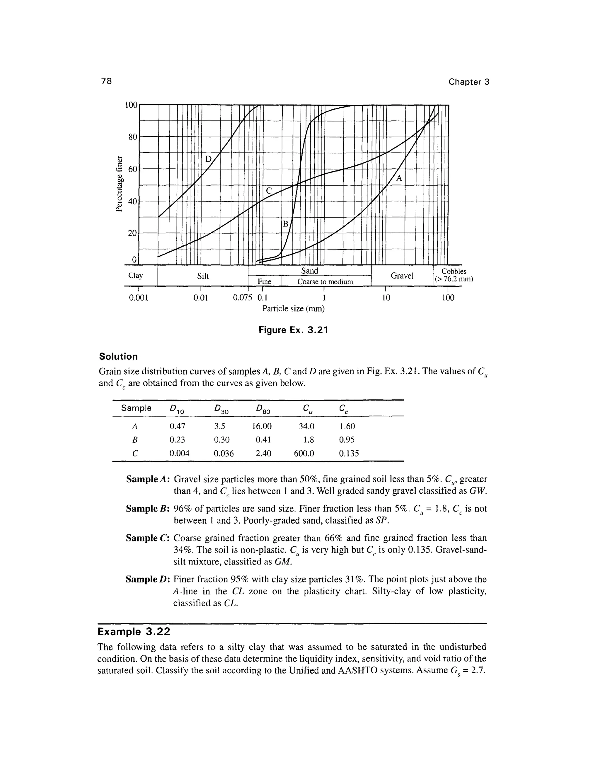
Example 3.2 1
Mechanical analysis on four different samples designated as A, B,C and D were carried out in a soil
laboratory. The results of tests are given below. Hydrometer analysis was carried out on sample D.
The soil is non-plastic.
Sample D: liquid limit = 42, plastic limit = 24, plasticity index =18
Classify the soils per the Unified Soil Classification System.
Samples
ASTM Sieve
Designation
63.0 mm
20.0 mm
6.3
2.0mm
600JL I
212 ji
63 ji
20 n
6(1
2 |i
A
Percentage
100
64
39
24
12
5
1
B
finer than
100
98
90
9
2
C
93
76
65
59
54
47
34
23
7
4
D
100
95
69
46
31

97. 78 Chapter 3
0.001 0.01 0.075 0. 1 1
Particle size (mm)
Figure Ex. 3.2 1
Cobbles
(> 76.2 mm)
100
Solution
Grain size distribution curves of samples A, B, C and D are given in Fig. Ex. 3.21. The values of Cu
and Cc are obtained fro m th e curves as given below.
Sample
A
B
C
D
10
0.47
0.23
0.004
^30
3.5
0.30
0.036
D
60
16.00
0.41
2.40
cu
34.0
1.8
600.0
cc
1.60
0.95
0.135
Sample A: Grave l size particles mor e than 50%, fin e grained soi l less than 5%. Cu, greater
than 4, and Cc lies between 1 and 3. Well graded sand y gravel classified as GW.
Sample/?: 96 % of particles ar e sand size. Finer fractio n less tha n 5%. C u = 1.8, C, is not
between 1 and 3. Poorly-graded sand , classified as SP.
Sample C: Coars e graine d fractio n greate r tha n 66 % an d fin e graine d fractio n les s tha n
34%. The soil is non-plastic. Cu is very high but Cc is only 0.135. Gravel-sand -
silt mixture, classified as CM.
Sample/): Finer fraction 95% with clay size particles 31% . The point plots just above the
A-line i n th e C L zon e o n th e plasticit y chart . Silty-cla y o f lo w plasticity ,
classified a s CL.
Example 3.2 2
The followin g dat a refer s t o a silt y cla y tha t wa s assume d t o b e saturate d i n th e undisturbe d
condition. On the basis of these data determine the liquidity index, sensitivity, and void ratio of the
saturated soil . Classify th e soil according t o the Unified and AASHTO systems. Assume G = 2.7.

98. Soil Phas e Relationships , Index Propertie s and Soil Classification 7 9
Index propert y Undisturbe d
Unconfmed compressive
strength, qu kN/m2
24 4 kN/m2
Water content, % 2 2
Liquid limit, %
Plastic limit, %
Shrinkage limit, %
% passing no. 200 sieve
Remolded
144 kN/m2
22
45
20
12
90
Solution
wn-w 22-2 0
Liquidity Index , / , = — =
= 0.08
' Wf-w 45-2 0
q undisturbe d 24 4
Sensitivity, 5 = —
= = 1.7
q'u disturbe d 14 4
V
Void ratio , e = —
V,
ForS=l,e = wGs = 0.22 x2.7 = 0.594.
Unified Soi l Classificatio n
Use the plasticity chart Fig. 3.22. w, = 45, / = 25. The point falls above the A-line in the CL-zone,
that is the soil is inorganic clay of low to medium plasticity.
AASHTO Syste m
Group Index GI = 0.2a + 0.005ac + 0.01 bd
a = 9
0 -35 =5
5
£ = 90-15 = 75
c = 45 ~40 =5
d = 25 -1 0 =15 (here Ip = wt - w p = 4
5 -20 =25)
Group index GI = 0.2 x 55 + 0.005 x 55 x 5 + 0.01 x 75 x 15
= 1 1 + 1.315+ 11.25 =23.63 or say 24
Enter Table 3.1 5 with the following data
% passing 200 sieve = 90 %
Liquid limit
= 45 %
Plasticity inde x
= 25 %
With this, the soil is either A-7-5 or A-7-6. Since (w l - 30 ) =(45 -30 ) =15 <25 (/ ) the soil
is classified as A-7-6. According to this system the soil is clay, A-7-6 (24).

99. 80 Chapte r 3
3.22 PROBLEM S
3.1 A soil mass in its natural state is partially saturated having a water content of 17.5% and a
void rati o o f 0.87 . Determin e th e degre e o f saturation , tota l uni t weight , an d dr y uni t
weight. What is the weight of water required to saturate a mass of 1 0 m3
volume? Assume
G^ = 2.69 .
3.2 Th e voi d rati o o f a clay sample i s 0.5 and the degree of saturation is 70%. Comput e th e
water content, dry and wet unit weights of the soil. Assume Gs = 2.7.
3.3 A sampl e o f soi l compacte d accordin g t o a standar d Procto r tes t ha s a uni t weigh t o f
130.9 lb/ft 3
a t 100 % compactio n an d at optimum wate r conten t o f 14% . Wha t i s the dry
unit weight? If the voids become filled with water what would be the saturated unit weight?
Assume Gs = 2.67.
3.4 A sample o f sand above th e water table was found to have a natural moisture conten t of
15% an d a uni t weigh t o f 18.8 4 kN/m 3
. Laborator y test s o n a drie d sampl e indicate d
values o f emin = 0.50 an d emax - 0.8 5 fo r th e denses t an d looses t state s respectively .
Compute the degree o f saturation and the relative density. Assume Gs = 2.65.
3.5 Ho w many cubic meters of fill can be constructed at a void ratio of 0.7 from 119,000 m3
of
borrow materia l that has a void ratio of 1.2 ?
3.6 Th e natural water content of a sample taken from a soil deposit wa s found to be 11.5% . It
has been calculated that the maximum density for the soil will be obtained when the water
content reaches 21.5%. Compute how much water must be added to 22,500 Ib of soil (in its
natural state ) in order t o increase th e water content to 21.5%. Assume tha t the degree of
saturation in its natural state was 40% and G = 2.7.
3.7 I n an oil well drilling project, drillin g mud was used to retain the sides of the borewell. I n
one liter of suspension in water, the drilling mud fluid consists o f the following material:
Material
Clay
Sand
Iron filing s
Mass
(g)
410
75
320
Sp.gr
2.81
2.69
7.13
Find the density of the drilling fluid o f uniform suspension.
3.8 I n a field exploration , a soil sample wa s collected i n a sampling tube of internal diamete r
5.0 cm below th e ground water table. The length of the extracted sampl e was 10. 2 cm and
its mass was 387 g. If Gy = 2.7, and the mass of the dried sample is 313 g, find the porosity,
void ratio, degree of saturation, and the dry density of the sample .
3.9 A saturated sample of undisturbed clay has a volume of 19.2 cm3
and weighs 32.5 g . After
oven drying , the weight reduces to 20.2 g. Determine th e following:
(a) water content, (b ) specific gravity, (c) void ratio, an d (d) saturated densit y of the clay
sample.
3.10 Th e natural total unit weight of a sandy stratum is 117.7 lb/ft3
an d has a water content of
8%. For determining of relative density, dried sand from the stratum was filled loosely int o
a 1.06 ft3
mold and vibrated to give a maximum density. The loose weight of the sample in
the mold wa s 105. 8 Ib , and the dense weigh t was 136. 7 Ib . If G9 = 2.66, fin d th e relativ e
density of the sand in its natural state.
3.11 A n earth embankment is to be compacted to a density of 120. 9 lb/ft 3
at a moisture conten t
of 1 4 percent . Th e in-sit u tota l uni t weigh t an d wate r conten t o f th e borro w pi t ar e

100. Soil Phas e Relationships , Index Propertie s and Soil Classification 8 1
114.5 lb/ft3
an d 8 % respectively. Ho w muc h excavatio n shoul d b e carrie d ou t fro m th e
borrow pit for each ft 3
of the embankment? AssumeG^ , = 2.68.
3.12 A n undisturbed sample of soil has a volume of 29 cm3
and weighs 48 g. The dry weight of
the sample is 32 g. The value of Gs = 2.66. Determine the (a) natural water content, (b) in-
situ void ratio, (c ) degree of saturation, and (d) saturated unit weight of the soil.
3.13 A mass o f soil coate d wit h a thin layer o f paraffin weigh s 0.982 Ib. When immerse d i n
water i t displaces 0.01130 2 ft 3
o f water . The paraffi n i s peele d of f an d foun d to weigh
0.0398 Ib . Th e specifi c gravit y o f th e soi l particle s i s 2. 7 an d tha t o f paraffi n i s 0.9 .
Determine the void ratio of the soil if its water content is 10%.
3.14 22 5 g of oven dried soil was placed in a specific gravity bottle and then filled with water to
a constant volume mark made on the bottle. The mass of the bottle with water and soil is
1650 g. The specific gravity bottle was filled with water alone to the constant volume mark
and weighed. Its mass was found to be 151 0 g. Determine the specific gravity of the soil.
3.15 I t is required to determine th e water content of a wet sample of silty sand weighing 400 g.
This mass of soil was placed in a pycnometer and water filled to the top of the conical cup
and weighed (M3). Its mass was found to be 2350 g. The pycnometer was next filled with
clean wate r and weighed and its mass was found t o be 2200 g (A/4). AssumingG^. = 2.67,
determine the water content of the soil sample.
3.16 A clay sample is found to have a mass of 423.53 g in its natural state. It is then dried in an
oven at 105 °C. The dried mass is found to be 337.65 g. The specific gravity of the solids is
2.70 and the density of the soil mass in its natural state is 1700 kg/m3
. Determine the water
content, degree o f saturation and the dry density of the mass in its natural state.
3.17 A sampl e o f san d i n it s natura l state has a relative densit y of 6 5 percent. Th e dr y unit
weights of the sample at its densest and loosest states are respectively 114. 5 and 89.1 lb/ft3
.
Assuming th e specifi c gravit y o f th e solid s a s 2.64 , determin e (i ) it s dr y uni t weight,
(ii) wet unit weight when fully saturated , and (iii) submerged unit weight.
3.18 Th e mass of wet sample of soil in a drying dish is 462 g. The sample and the dish have a
mass of 364 g after drying in an oven at 11 0 °C overnight. The mass of the dish alone is
39 g. Determine the water content of the soil.
3.19 A sample o f sand above th e water table wa s found to have a natural moisture content of
10% and a unit weight of 12 0 lb/ft3
. Laboratory test s on a dried sampl e indicate d value s
e
mm ~ 0-45, and emax = 0.90 fo r the densest an d loosest state s respectively. Comput e th e
degree o f saturation, S, and the relative density, Df. Assum e G^ = 2.65.
3.20 A 50 cm3
sample of moist clay was obtained by pushing a sharpened hollo w cylinder into
the wall of a test pit. The extruded sample had a mass of 85 g, and after oven drying a mass
of 60 g. Compute w, e, S, and pd. Gs = 2.7.
3.21 A pit sample o f moist quartz sand was obtained fro m a pit by the sand cone method. Th e
volume of the sample obtained was 150 cm3
and its total mass was found to be 250 g. In the
laboratory th e dry mas s o f the sand alone wa s found t o be 240 g. Tests on the dry sand
indicated emax = 0.80 and emin =0.48. Estimate ps, w, e, S, pd and Dr of the sand in the field.
Given Gs = 2.67.
3.22 A n earthen embankmen t unde r construction has a total uni t weight o f 99.9 lb/ft 3
an d a
moisture content of 1 0 percent. Comput e the quantity of water required t o be added pe r
100 ft3
of earth to raise its moisture content to 14 percent a t the same void ratio.
3.23 Th e wet unit weight of a glacial outwash soil is 122 lb/ft3
, the specific gravity of the solids
is GS = 2.67, an d the moisture content of the soil is w = 12% by dry weight. Calculate (a )
dry unit weight, (b) porosity, (c) void ratio, and (d ) degree of saturation.

101. 82 Chapter 3
3.24 Deriv e the equation e = wGs which expresses th e relationship between th e void ratio e, the
specific gravity Gs and the moisture content w for full saturatio n of voids.
3.25 I n a sieve analysis of a given sample of sand the following data were obtained . Effective
grain size = 0.25 mm, uniformity coefficient 6.0, coefficient of curvature =1.0 .
Sketch the curve on semilog paper.
3.26 A sieve analysis of a given sample o f sand was carried ou t by making use of US standar d
sieves. The total weight of sand used for the analysis was 522 g. The following data were
obtained.
Sieve size in mm 4.75 0 2.00 0 1.00 0 0.50 0 0.35 5 0.18 0 0.12 5 0.07 5
Weight retained
ing 25.7 5 61.7 5 67.00126. 0 57.7 5 78.7 5 36.7 5 36.7 5
Pan 31. 5
Plot the grain size distribution curve on semi-log paper an d compute the following:
(i) Percen t grave l
(ii) Percen t of coarse, medium and fine san d
(iii) Percen t of silt and clay
(iv) Uniformit y coefficient
(v) Coefficien t of curvature
3.27 Combine d mechanica l analysis of a given sample of soil was carried out. The total weight
of soi l use d i n th e analysi s wa s 35 0 g . The sampl e wa s divide d int o coarse r an d fine r
fractions b y washin g i t throug h a 7 5 micron s siev e Th e fine r tractio n wa s 12 5 g. Th e
coarser fraction was used for the sieve analysis and 50 g of the finer fraction was used for
the hydrometer analysis. The test results were as given below:
Sieve analysis:
Particle size
4.75 m m
2.00 m m
1.40 m m
1.00mm
500 fi
Mass retained g
9.0
15.5
10.5
10.5
35.0
Particle size
355 u
180 n
125 u
75 n
Mass
24.5
49.0
28.0
43.0
retained g
A hydrometer (15 2 H type) was inserted into the suspension just a few seconds before th e
readings were taken. It was next removed and introduced just before each of the subsequent
readings. Temperature of suspension = 25°C.
Hydrometer analysis : Reading s in suspensio n
Time, mi n
1/4
1/2
1
2
4
8
15
Reading, Rg
28.00
24.00
20.50
17.20
12.00
8.50
6.21
Time, min
30
60
120
240
480
1440
Reading, Rg
5.10
4.25
3.10
2.30
1.30
0.70

102. Soil Phas e Relationships, Inde x Propertie s an d Soil Classification 8 3
Meniscus correction C m = +0.4, zero correction C o = +l.5,Gs = 2.75
(i) Sho w (step by step) all the computations required for the combined analysis ,
(ii) Plo t the grain size distribution curve on semi-log paper
(iii) Determin e the percentages of gravel, sand, and fine fractions present in the sample
(iv) Comput e the uniformity coefficient an d the coefficient o f curvature
(v) Commen t on the basis of the test results whether the soil is well graded or not
3.28 Liqui d limit tests were carried out on two given samples of clay. The test data are as given
below.
Test Nos
Sample no. 1
Water content %
Number of blows, N
Sample no. 2
Water content %
Number of blows, N
1
120
7
96
9
2
114
10
74
15
3
98
30
45
32
4
92
40
30
46
The plastic limit of Sample No. 1 is 40 percent and that of Sample No. 2 is 32 percent.
Required:
(i) The flow indices of the two samples
(ii) The toughness indices of the samples
(iii) Comment on the type of soils on the basis of the toughness index values
3.29 Fou r different type s of soils were encountered in a large project. Their liquid limits (w;),
plastic limits (w ) and their natural moisture contents (wn) were as given below:
Soil type
1
2
3
4
w,%
120
80
60
65
wp%
40
35
30
32
wn%
150
70
30
25
Required:
(i) The liquidity indices of the soils, (ii) the consistency of the natural soils (i.e., whether soft,
stiff, etc.)
(ii) and the possible behavior of the soils under vibrating loads
3.30 Th e soil type s as given in Problem 3.2 9 contained soi l particles finer than 2 microns as
given below:
Soil typ e
Percent finer
than 2 micron
1
50
2
55
3
45
4
50
Classify th e soils according to their activity values.

103. 84 Chapter 3
3.31 A sample of clay has a water content of 40 percent at full saturation . Its shrinkage limit is
15 percent . Assumin g G s = 2.70, determin e it s degre e o f shrinkage . Commen t o n th e
quality of the soil.
3.32 A sample of clay soil has a liquid limit of 62% and its plasticity index is 32 percent.
(i) Wha t i s the state of consistency of the soil if the soil in its natural state has a water
content of 34 percent?
(ii) Calculat e the shrinkage limit if the void ratio of the sample a t the shrinkage limit is
0.70
Assume G ^ = 2.70 .
3.33 A soil with a liquidity index of-0.20 has a liquid limit of 56 percent and a plasticity index
of 20 percent. What is its natural water content?
3.34 A sampl e o f soi l weighin g 5 0 g i s disperse d i n 100 0 m L o f water . Ho w lon g afte r th e
commencement o f sedimentatio n shoul d th e hydromete r readin g b e take n i n orde r t o
estimate th e percentage of particles less than 0.002 mm effective diameter, i f the center of
the hydrometer i s 150 mm below the surface of the water?
Assume: Gs = 2.1; ^ = 8.15 x 10"6
g-sec/cm 2
.
3.35 Th e results of a sieve analysis of a soil were as follows:
Sieve
size (mm )
20
12
10
6.3
4.75
2.8
Mass
retained (g)
0
1.7
2.3
8.4
5.7
12.9
Sieve
size (mm )
2
1.4
0.5
0.355
0.180
0.075
Mass
retained (g)
3.5
1.1
30.5
45.3
25.4
7.4
The total mass of the sample was 147. 2 g.
(a) Plo t the particle-size distribution curve and describe th e soil. Comment o n the flat part
of the curve
(b) Stat e the effective grai n size
3.36 A liquid limit test carried out on a sample of inorganic soil taken from below the water table
gave the following results:
Fall cone penetration y (mm) 15. 5 18. 2 21. 4 23. 6
Moisture content, w% 34. 6 40. 8 48. 2 53. 4
A plastic limit test gave a value of 33%. Determine th e average liquid limit and plasticity
index of this soil and give its classification.
3.37 Th e ove n dr y mas s o f a sample o f clay was 11.2 6 g. The volum e o f the dry sampl e wa s
determined b y immersing it in mercury and the mass of the displaced liqui d was 80.29 g.
Determine the shrinkage limit, vvy, of the clay assuming Gs = 2.70.

104. Soil Phas e Relationships , Inde x Propertie s an d Soil Classification 8 5
3.38 Particle s of five different sizes are mixed in the proportion shown below and enough water
is added to make 100 0 cm3
of the suspension.
Particle siz e (mm )
0.050
0.020
0.010
0.005
0.001
Mass (g)
6
20
15
5
4 Total 50 g
It is ensured that the suspension is thoroughly mixed so as to have a uniform distribution of
particles. All particles have specific gravity of 2.7.
(a) Wha t is the largest particle size present at a depth of 6 cm after 5 mins from the start of
sedimentation?
(b) Wha t is the density of the suspension at a depth of 6 cm after 5 mins from th e start of
sedimentation?
(c) Ho w long should sedimentation be allowed so that all the particles have settled below
6 cm? Assume ,u= 0.9 x 1Q- 6
kN-s/m2
3.39 A sample of clayey silt is mixed at its liquid limit of 40%. It is placed carefully in a small
porcelain dish with a volume of 19.3 cm3
and weighs 34.67 g. After oven drying, the soil
pat displaced 216. 8 g of mercury.
(a) Determine the shrinkage limit, ws, of the soil sample
(b) Estimate the dry unit weight of the soil
3.40 Durin g the determination of the shrinkage limit of a sandy clay, the following laboratory
data was obtained:
Wet wt. of soil + dish
= 87.8 5 g
Dry wt. of soil + dish
= 76.9 1 g
Wt of dish
= 52.7 0 g
The volumetric determination o f the soil pat:
Wt. of dish + mercury
= 430. 8 g
Wt. of dish
= 244.62 g
Calculate the shrinkage limit, assuming Gs
= 2.6 5
3.41 A sedimentation analysis by a hydrometer (152 H type) was conducted with 50 g of oven
dried soil sample. The hydrometer reading in a 1000 cm3
soil suspension 60 mins after the
commencement o f sedimentatio n i s 19.5 . Th e meniscu s correctio n i s 0.5 . Assumin g
Gs = 2.70 an d L - 1 x 10" 6
kN-s/m2
for water, calculate the smallest particl e siz e which
would have settled during the time of 60 mins and percentage o f particles finer than this
size. Assume: C0 = +2.0, and CT = 1.2
3.42 Classif y the soil given below using the Unified Soil Classification System.
Percentage passing No. 4 sieve 7 2
Percentage passing No. 200 sieve 3 3
Liquid limit 3 5
Plastic limit 1 4

105. 86 Chapte r 3
3.43 Soi l samples collecte d from th e field gave the following laboratory tes t results:
Percentage passin g No. 4 sieve 10 0
Percentage passin g No. 200 sieve 1 6
Liquid limit 6 5
Plastic limit 3 0
Classify th e soil using the Unified Soil Classification System .
3.44 Fo r a large project, a soil investigation was carried out. Grain size analysis carried out on
the samples gav e the following average tes t results.
Sieve No . Percen t finer
4 9 6
10 6 0
20 1 8
40 1 2
60 7
100 4
200 2
Classify th e soil by using the Unified Soi l Classification System assuming the soil is non-
plastic.
3.45 Th e sieve analysis of a given sample of soil gave 57 percent of the particles passing through
75 micro n sieve . Th e liqui d an d plasti c limit s o f th e soi l wer e 6 2 an d 2 8 percen t
respectively. Classif y th e soi l pe r th e AASHT O an d th e Unifie d Soi l Classificatio n
Systems.

106. CHAPTER 4
SOIL PERMEABILITY AND SEEPAGE
4.1 SOI L PERMEABILIT Y
A material is permeable if it contains continuous voids. All materials such as rocks, concrete, soil s
etc. ar e permeable . Th e flo w o f water through all of them obey s approximatel y th e sam e laws .
Hence, the difference between the flow o f water through rock o r concrete i s one of degree. The
permeability o f soil s has a decisive effec t o n the stabilit y of foundations, seepage los s throug h
embankments of reservoirs, drainage of subgrades, excavation of open cuts in water bearing sand,
rate of flow o f water into wells and many others.
Hydraulic Gradien t
When water flows through a saturated soil mass there is certain resistance fo r the flow because of
the presence of solid matter. However, the laws of fluid mechanics which are applicable for the flow
of fluid s throug h pipe s ar e als o applicabl e t o flo w o f wate r throug h soils . A s pe r Bernoulli's
equation, th e total head at any point in water under steady flow condition may be expressed as
Total head = pressure head + velocity head + elevation head
This principle can be understood with regards to the flow of water through a sample of soil
of length L and cross-sectional are a A as shown in Fig. 4.1 (a). The heads of water at points A and
B as the water flows from A to B are given as follows (with respect t o a datum)
Total head at A, H. = ZA + —^ + -^-
Y 2g
p V 2
Total head at B, H K
= ZK-—— + ——
87

107. 88 Chapter 4
Figure 4.1 (a) Flo w o f wate r throug h a sample of soi l
As the water flows from A to B, there is an energy loss which is represented b y the difference
in the total heads H, an d H D
or
H A-HB
= ZA
PA PR»
c
o u i _ ,
where, pA an d pB = pressure heads, V A and VB = velocity, g - acceleratio n due to gravity, yw = unit
weight of water, h = loss of head.
For all practical purposes the velocity head is a small quantity and may be neglected. The loss
of head of h units is effected as the water flows from A to B. The loss of head per unit length of flow
may be expressed as
h
i = (4.1)
where / is called the hydraulic gradient.
Laminar an d Turbulent Flo w
Problems relating to the flow o f fluids in general may be divided into two main classes:
1. Thos e in which the flow is laminar.
2. Thos e in which the flow i s turbulent.
There i s a certain velocity, vc, below which for a given diameter of a straight tube and for a
given flui d a t a particular temperature, the flow wil l always remain laminar . Likewise there i s a
higher velocity, vr above which the flow will always be turbulent. The lower bound velocity, vp of
turbulent flo w i s abou t 6. 5 time s th e uppe r boun d velocit y v o f lamina r flo w a s show n i n
Fig. 4.1(b). The uppe r boun d velocity of laminar flow i s called th e lower critical velocity. Th e
fundamental law s tha t determin e th e stat e existin g fo r an y give n cas e wer e determine d b y
Reynolds (1883). H e found the lower critical velocity is inversely proportional to the diameter of

108. Soil Permeability and Seepage 89
log/
Flow always
Flow always laminar -
laminar turbulen t Flow alway s
turbulent
VT
logv
Figure 4.Kb) Relationshi p betwee n velocit y of flow and hydraulic gradien t fo r flow
of liquid s in a pipe
the pipe and gave the following general expression applicable for any fluid an d for any system of
units.
= 2000
where, A ^ = Reynold s Numbe r take n a s 200 0 a s th e maximu m valu e for th e flo w t o remai n
always laminar, D = diameter of pipe, vc = critical velocity below which the flow always remains
laminar, y 0 = unit weight of fluid a t 4 °C,fJL = viscosity of fluid, g = acceleration du e t o gravity.
The principal difference between laminar flow an d turbulent flow i s that in the former case
the velocity is proportional to the first power of the hydraulic gradient, /, whereas in the latter case
it is 4/7 the power of /. According to Hagen-Poiseuille's' Law the flow through a capillary tube may
be expressed a s
R2
ai
(4.2a)
or (4.2b)
where, R = radius of a capillary tube of sectional area a, q = discharge through the tube, v = average
velocity through the tube, ^ = coefficient of viscosity.
4.2 DARCY' S LAW
Darcy in 185 6 derive d an empirical formula for the behavior o f flow throug h saturated soils . H e
found tha t the quantit y of wate r q per se c flowing through a cross-sectional are a of soi l under
hydraulic gradient / can be expressed b y the formula
q = kiA
or the velocity of flow can be written as
(4.3)

109. 90 Chapter 4
1 .0
1.6
1.4
1.0
0.8
n £
^^k^
10 2 0
Temperature ° C
30
Figure 4.2 Relatio n between temperature an d viscosity of wate r
v = -j = & (4.4 )
where k is termed th e hydraulic conductivity (o r coefficient o f permeability)with units of velocity. A
in Eq. (4.4) is the cross-sectional area of soil normal to the direction of flow which includes the area of
the solids and the voids, whereas the area a in Eq. (4.2) is the area of a capillary tube. The essential
point i n Eq . (4.3 ) i s tha t the flo w throug h the soil s i s als o proportiona l t o th e firs t powe r o f th e
hydraulic gradient i as propounded by Poiseuille's Law. From this, we are justified in concluding that
the flow of water through the pores o f a soil is laminar. It is found that, on the basi s o f extensive
investigations made since Darcy introduced his law in 1856, this law is valid strictly for fine grained
types of soils.
The hydrauli c conductivit y i s a measur e o f th e eas e wit h whic h wate r flow s throug h
permeable materials . I t is inversel y proportional t o the viscosit y of wate r whic h decreases with
increasing temperature as shown in Fig. 4.2. Therefore, permeabilit y measurements at laboratory
temperatures should b e corrected with the aid of Fig. 4.2 before applicatio n t o fiel d temperatur e
conditions by means of the equation
k ~ ~
(4.5)
where k f an d k T ar e th e hydrauli c conductivit y value s correspondin g t o th e fiel d an d tes t
temperatures respectively and /^,and ^rare the corresponding viscosities . It is customary to report
the values of kT at a standard temperature of 20°C. The equation is
^20
(4.6)
4.3 DISCHARG E AN D SEEPAG E VELOCITIES
Figure 4. 3 shows a soil sampl e o f length L and cross-sectional are a A. The sample i s placed i n a
cylindrical horizontal tube between screens. The tube is connected t o two reservoirs R^ an d R2 in
which the water levels are maintained constant. The difference in head between R{ an d R2 is h. This
difference i n head is responsible for the flow of water. Since Darcy's law assumes no change in the

110. Soil Permeability and Seepag e 91
Screen
— Sample
B
Screen
Figure 4.3 Flo w of water through a sample of soi l
volume of voids and the soil is saturated, the quantity of flow past sections AA, BB and CC should
remain the same for steady flow conditions. We may express the equation of continuity as follows
Qaa = <lbb = 3cc
If the soil be represented a s divided into solid matter and void space, then the area available
for th e passage of wate r is only Av. If vs is the velocit y of flow i n the voids , an d v , the averag e
velocity across the section then, we have
A v = Av o r v = —v
s
A
A 1 l + e
Since, ~7 ~ = ~=
A.. n e
+ e
(4.7)
Since (1 + e)le i s always greater than unity, vs is always greater than v. Here, vs is called the
seepage velocity and v the discharge velocity.
4.4 METHOD S O F DETERMINATION O F HYDRAULIC
CONDUCTIVITY O F SOILS
Methods that are in common use for determining the coefficient of permeability k can be classified
under laboratory and field methods.
Laboratory methods:
Field methods :
Indirect Method:
1. Constant head permeability method
2. Falling head permeability method
1. Pumping tests
2. Bore hole tests
Empirical correlation s
The various types of apparatus which are used in soil laboratories for determining the permeability of
soils are called permeameters. The apparatus used for the constant head permeability test is called a
constant head permeameter and the one used for the falling head test is a fallingheadpermeameter.
The soi l sample s use d i n laborator y method s ar e eithe r undisturbe d or disturbed . Sinc e i t i s not

111. 92 Chapter 4
possible t o obtai n undisturbe d sample s o f cohesionles s soils , laborator y test s o n cohesionles s
materials are always conducted on samples which are reconstructed to the same density as they exist
in nature. The results of tests on such reconstructed soils are often misleading since it is impracticable
to obtain representative samples and place them in the test apparatus to give exactly the same density
and structural arrangement of particles. Direct testing of soils in place is generally preferred i n cases
where i t i s no t possibl e t o procur e undisturbe d samples. Sinc e thi s metho d i s quit e costly , i t i s
generally carried ou t in connection with major projects such as foundation investigation for dams and
large bridges o r building foundation jobs where lowering of the water table is involved. In place of
pumping tests, bore hole tests as proposed by the U.S. Bureau of Reclamation are quite inexpensive as
these tests eliminate the use of observation wells.
Empirical correlation s hav e been develope d relatin g grain size an d voi d ratio to hydraulic
conductivity and will be discussed later on.
4.5 CONSTAN T HEA D PERMEABILITY TEST
Figure 4.4(a) shows a constant head permeameter whic h consists of a vertical tube of lucite (or any
other material) containing a soil sample which is reconstructed o r undisturbed as the case may be.
The diameter and height of the tube can be of any convenient dimensions. The head and tail water
levels ar e kep t constan t b y overflows . Th e sampl e o f lengt h L an d cross-sectiona l are a A i s
subjected to a head h which is constant during the progress of a test. A test is performed by allowing
water to flow through the sample and measuring the quantity of discharge Q in time t.
The value of k can be computed directly from Darcy' s law expressed a s follows
Supply
, c -
Screen
.Soil
sample
Filter skin
Graduated jar
~
T
h
1
(a) (b )
Figure 4.4 Constan t hea d permeability tes t

112. Soil Permeability and Seepage 9 3
Q = k—At (4.8 )
01
=
<4
-9
>
The constant head permeameter test is more suited for coarse grained soils such as gravelly sand
and coarse and medium sand. Permeability tests in the laboratory are generally subjected to various
types of experimental errors. One of the most important of these arises from the formation of a filter
skin of fine materials on the surface of the sample. The constant head permeameter of the type shown
in Fig. 4.4(b) can eliminate the effect of the surface skin. In this apparatus the loss of head is measured
through a distance in the interior of the sample, and the drop in head across the filter skin has no effect
on the results.
4.6 FALLIN G HEA D PERMEABILIT Y TES T
A falling head permeameter is shown in Fig. 4.5(a). The soil sample is kept in a vertical cylinder of
cross-sectional are a A. A transparent stand pipe of cross sectiona l area , a, is attached to the test
cylinder. The test cylinder is kept in a container filled with water, the level of which is kept constant
by overflows. Before the commencement o f the test the soil sample is saturated by allowing the
water to flow continuously through the sample from the stand pipe. After saturation is complete, the
stand pipe is filled with water up to a height of hQ and a stop watch is started. Let the initial time be
tQ. The time tl when the water level drops from hQ to h} is noted. The hydraulic conductivity k can be
determined on the basis of the drop in head (hQ - hj an d the elapsed time (tl - ?0) required for the drop
as explained below.
Let h be the head of water at any time t. Let the head drop by an amount dh in time dt. The
quantity of water flowing through the sample in time dt from Darcy's law is
h
dQ = kiAdt= k—Adt(4.10 )
Lv
'
where, i = h/L the hydraulic gradient.
The quantity of discharge dQ can be expressed as
dQ = -adh(4.11 )
Since the head decreases as time increases, dh is a negative quantity in Eq. (4.11). Eq. (4.10)
can be equated to Eq. (4.11)
h
-adh = k— Adt(4.12 )
The discharg e Q i n tim e (t^ - f Q) ca n b e obtaine d b y integratin g Eq . (4.10 ) o r (4.11) .
Therefore, Eq. (4.12) can be rearranged and integrated as follows
*i
Cdh kA C h n kA
-a — = — d t o r ' - °
The general expression for k is

113. 94 Chapter 4
dh
T Stand pipe
1
L
I
E!
#Vc?**£
"X'^;<V
J?
k'v's&S
/> Scree
J
Sample
(a) (b )
Figure 4.5 Fallin g hea d permeabilit y tes t
k =
aL
A(t,
or k =
23aL
(4.13)
The setup shown in Fig. 4.5(a) is generally used for comparatively fine materials such as fine
sand and silt where the time required for the drop in head from hQ to hl i s neither unduly too long
nor too short for accurate recordings. If the time is too long evaporation of water from the surface of
the water might take place and also temperature variations might affect th e volume of the sample .
These woul d introduc e seriou s error s i n th e results . Th e se t u p i s suitabl e fo r soil s havin g
permeabilities rangin g from 10~ 3
to 10~ 6
cm pe r sec . Sometimes , fallin g hea d permeameter s ar e
used for coarse graine d soils also. For such soils, the cross sectiona l are a of the stand pipe is made
the sam e a s the test cylinde r so that the drop i n head ca n conveniently be measured . Fig . 4.5(b )
shows the test set up for coarse grained soils. When a = A, Eq. (4.13) is reduced to
2.3L , h Q
log,n — (4.14)
Example 4. 1
A constant head permeability test was carried ou t on a cylindrical sample of sand 4 in. in diamete r
and 6 in. in height. 1 0 in3
of water was collected i n 1.7 5 min, under a head o f 1 2 in. Compute th e
hydraulic conductivity in ft/year and the velocity of flow i n ft/sec.
Solution
The formul a for determining k is
Ait

114. Soil Permeability an d Seepage 9 5
42
Q = 10 in3
, A = 3.14 x — = 12.56 in. 2
7 1 O
i = — =— = 2, t = 105 sec.
L 6
Therefore f c =
= 3.79 x 10~3
in./se c = 31.58 x 10~5
ft/se c = 9960 ft/yea r
12.56x2x105
Velocity of flow = Id =31.58 x10~5
x2 = 6.316 x 10~4
ft/se c
Example 4. 2
A san d sampl e o f 3 5 cm 2
cros s sectiona l are a an d 2 0 c m lon g wa s teste d i n a constan t hea d
permeameter. Unde r a head of 60 cm, the discharge wa s 120 ml in 6 min. The dry weight of sand
used for the test was 1 120 g, and Gs =2.68. Determine (a) the hydraulic conductivity in cm/sec, (b)
the discharge velocity , and (c) the seepage velocity .
Solution
Use Eq. (4.9), k = —
hAt
where Q = 120 ml, t = 6 min, A = 35 cm2
, L = 20 cm, and h = 60 cm. Substituting, we have
k = -
=3.174 x10~3
cm/se c
60x35x6x60
Discharge velocity, v = ki = 3.174 x 10~3
x — = 9.52 x 10~3
cm/se c
Seepage velocity vs
W 112 0
Y G G
From Eq. (3.1 8a), Y f t ~ w s o r e
~ — ~~^sinc e y = 1 g/cm3
l + ey d
Substituting, e = — - - 1 =0.675
1.6
0.675
= 0.403
l + e1 + 0.675
v 952xlO~ 3
Now, v = — =
— '•
= 2.36 x 10"2
cm/se c
J
n 0.40 3
Example 4. 3
Calculate the value ofA: of a sample of 2.36 in. height and 7.75 in2
cross-sectional area , if a quantity
of water of 26.33 in3
flows down in 1 0 min under an effective constan t head of 15.7 5 in. On oven

115. 96 Chapte r 4
drying, the test specimen weighe d 1. 1 Ib. Assuming Gs = 2.65, calculat e the seepag e velocit y of
water during the test.
Solution
From Eq. (4.9), k = ^-= -
2633x23
6
-
=0.8x 10~3
in./se c
hAt 15.75x7.75x10x6 0
Discharge velocity, v =ki = k— = 0.8xlO~3
x — :
—= 5.34xlO~3
in./sec
L 2.3 6
W 1 1
Y = —s- = -
: -
= 0.0601 lb/in3
=103.9 lb/ft 3
d
V 7.75x2.3 6
Y G
FromEq. (3.18a) , e = ^-^—
Yd
62.4x2.65
or e - -
-- 1 = 0.59 1 5
103.9
°-5915
= 0.37 2
l + e1 + 0.5915
v 5.3 4 xlO~3
Seepage velocity, v =— =
— -
=14.3
5 x10~3
in./sec
6 s
n 0.37 2
Example 4. 4
The hydrauli c conductivity of a soi l sampl e wa s determine d i n a soi l mechanic s laborator y b y
making us e o f a falling hea d permeameter. The dat a used an d th e tes t results obtaine d wer e as
follows: diameter of sample = 2.36 in, height of sample = 5.91 in, diameter of stand pipe = 0.79 in,
initial head h Q = 17.72 in. final hea d hl = 11.81 in. Time elapse d = 1 min 45 sec. Determin e the
hydraulic conductivity i n ft/day .
Solution
The formula for determining k is [Eq. (4.13)]
, . , , .
k = -
log,0 — -
where tis the elapsed time.
A • 3.14x0.79x0.7 9 0 . 1 A 4 ,2
Area of stand pipe, a = -
= 34 x 1
0 4
ft ^
4x12x12
Area of sample, A = 3
-14x2
-36x236
= 304 x 10~4
ft 2
4x12x12
Height of sample, L =(17
-72
~1L81
) = 04925 ft
1 772 118 1
Head, /z n = -^— = 1.477 ft, h, = —
= 0.984 ft
0
1 2 ]
1 2

116. Soil Permeability and Seepage 9 7
Elapsed time, t = 105 sec =
= 12.15 x 10~4
day s
60x60x24
2.3x34x10-4x0.4925 , 1.47 7 t f t f l j
k = x log
= 18 ft/day
304 x10-4
x 12.15 x ID"4
0.98 4
4.7 DIREC T DETERMINATIO N O F k O F SOILS I N PLAC E BY
PUMPING TES T
The most reliable information concerning the permeability of a deposit of coarse grained material
below the water table can usually be obtained by conducting pumping tests in the field. Although
such tests have their most extensive application in connection with dam foundations, they may also
prove advisable on large bridge or building foundation jobs where the water table must be lowered.
The arrangement consists of a test well and a series of observation wells. The test well is sunk
through the permeable stratum up to the impermeable layer. Awell sunk into a water bearing stratum,
termed a n aquifer, an d tapping free flowin g groun d water having a free groun d water table under
atmospheric pressure, is termed a gravity or unconfined well. A well sunk into an aquifer where the
ground water flow i s confined between two impermeable soi l layers, and is under pressure greate r
than atmospheric , i s termed a s artesian or confined well. Observation well s are drilled at various
distances from th e test or pumping well along two straight lines, one oriented approximately in the
direction of ground water flow and the other at right angles to it. A minimum of two observation wells
and their distances from the test well are needed. These wells are to be provided on one side of the test
well in the direction of the ground water flow.
The test consists of pumping out water continuously at a uniform rate from the test well until the
water levels in the test and observation wells remain stationary. When this condition is achieved the
water pumped out of the well is equal to the inflow into the well from the surrounding strata. The water
levels in the observation wells and the rate of water pumped out of the well would provide the necessary
additional data for the determination of k.
As the water from the test well is pumped out, a steady state will be attained when the water
pumped out will be equal to the inflow into the well. At this stage the depth of water in the well will
remain constant. The drawdow n resulting due to pumping is called th e cone of depression. Th e
maximum drawdown DQ is in the test well. It decreases with the increase in the distance from th e
test well. The depression dies out gradually and forms theoretically, a circle around the test well
called the circle of influence. The radius of this circle, /?., is called th e radius of influence o f the
depression cone .
Equation fo r k fo r a n Unconfine d Aquife r
Figure 4.6 gives the arrangement of test and observation wells for an unconfined aquifer. Only two
observation wells at radial distances of r{ and r2 from the test well are shown. When the inflow of
water int o the tes t wel l i s steady , the depth s o f water i n these observation well s ar e h{ an d h2
respectively.
Let h be the depth of water at radial distance r. The area of the vertical cylindrical surface of
radius r and depth h through which water flows is
A = Inrh
The hydraulic gradient is i = —
dr

117. 98
Ground level Test well
Chapter 4
Observation well s
Figure 4.6 Pumpin g tes t in an unconfined aquife r
As per Darcy's la w the rate of inflow into the well when the water levels in the wells remai n
stationary is
q = kiA
Substituting for A and / the rate of inflow acros s th e cylindrical surface i s
, dh^ ,
q - k — 2nrh
dr
Rearranging the terms, we have
dr Inkhdh
r q
The integral of the equation within the boundary limits is
dr Ink
r q .
hdh (4.15)
The equatio n for k after integratio n and rearranging is
k = - (4.16)
Proceeding i n th e sam e wa y a s befor e anothe r equatio n fo r k i n term s o f r Q, h Q and R { ca n b e
established a s (referring to Fig. 4.6
)

118. Soil Permeability an d Seepag e 99
2.3<?/?, -
* log- 1
- (4.17)
If we write hQ = (H-D 0) in Eq. (4.17), where DQ is the depth of maximum drawdown in the
test well, we have
2.3 q
-log^-
Y
0
Now from Eq. (4.18), the maximum yiel d from the well may be written as
_7rD0k(2H-DQ)I
q
~ 2 3
(4.18)
(4.19)
Radius of Influence R^ Base d on experience , Sichard t (1930 ) gav e an equatio n for
estimating the radius of influence for the stabilized flow condition as
/?. = 3000D0V& meter s (4.20)
where DQ = maximum drawdown in meters
k = hydraulic conductivity in m/sec
Equation fo r k i n a Confine d Aquife r
Figure 4. 7 show s a confine d aquife r wit h th e tes t an d observatio n wells . Th e wate r i n th e
observation wells rises above the top of the aquifer due to artesian pressure. When pumping from
such an artesian well two cases might arise. They are:
Case 1. The water level in the test well might remain above the roof leve l o f the aquifer at
steady flow condition.
Observation well s
Piezometnc
level during pumpin g
Case 1 h0 > H0
Case 2h0<H0
Impermeable
Impermeable stratum
Figure 4.7 Pumpin g test in confined aquife r

119. 100 Chapte r 4
Case 2. The water level in the test well might fall below the roof level of the aquifer at steady
flow condition .
If HQ is the thickness of the confined aquifer and hQ is the depth of water in the test well at the
steady flo w condition Case 1 and Case 2 may be stated as—
Casel. When/z 0>//0. Cas e 2. When/i Q<//0.
Case 1 . Whe n h 0 > H 0
In this case, the area of a vertical cylindrical surface of any radius r does not change, since the depth
of the water bearing strata is limited to the thickness HQ. Therefore, th e discharge surfac e area is
(4.21)
A • • • . dh . ~ . _ , ,
Again writing i - — , the now equation as per Darcy s law is
dr
dh_
dr °
The integration of the equation after rearranging the terms yield s
dr_ a r
— o r (A 2-/i1) = Tr7^1og,— (4-22 )
The equation for k is
, . ,
k = -
log
2 -A,) r ,
Alternate Equation s
As before w e can write the following equation for determining k
23q r ,
k =
iu ti. —T
T log
~~ (4.24a )
-^ '
, .
or k- -
- -
log— 1
-
, . t
OF
2xH D g
~r~
27rHQL>0 r 0
Case 2 . Whe n h 0 < H 0
Under the condition when hQ is less than HQ, the flow pattern close to the well is similar to that of an
unconfmed aquife r whereas at distances farther from the well the flow i s artesian. Muska t (1946 )
developed a n equation to determine the hydraulic conductivity. The equation is
*,-
— log — L

120. Soil Permeability and Seepag e 101
4.8 BOREHOL E PERMEABILIT Y TEST S
Two types of tests may be carried out in auger hole s for determining k. They are
(a) Fallin g water level method
(b) Risin g water level method
Falling Water Leve l Metho d (case d hol e an d soil flush with bottom )
In thi s test auge r holes ar e made in the field that extend belo w th e water tabl e level . Casing is
provided down to the bottom of the hole (Fig. 4.8(a)). The casing is filled with water which is then
allowed t o see p int o the soil . The rat e o f dro p o f the wate r level i n th e casin g i s observe d b y
measuring the depth of the water surface below the top of the casing at 1, 2 and 5 minutes after the
start of the test and at 5 minutes intervals thereafter. These observations are made until the rate of
drop become s negligibl e o r unti l sufficien t reading s hav e bee n obtained . Th e coefficien t o f
permeability is computed as [Fig. 4.8(a)]
2-3 nrQ H {
k = —log— -
-f,) ff ,
(4.26)
where, H{ = piezometric head ait = tl,H2 = piezometric head at t - t 2-
Rising Wate r Leve l Metho d (case d hol e an d soil flus h with bottom )
This method, most commonly referred to as the time-lag method, consists of bailing the water out
of the casing and observing the rate of rise of the water level in the casing at intervals until the rise
in water level becomes negligible. The rate is observed by measuring the elapsed time and the depth
of the water surface below the top of the casing. The intervals at which the readings are required
will vary somewhat with the permeability of the soil. Eq. (4.26) is applicable fo r this case, [Fig
.
4.8(b)]. A rising water level test should always be followed by sounding the bottom of the holes to
determine whether the test created a quick condition.
HI a t t =
H a t t = t
(a) Falling water head method (b ) Rising water head method
Figure 4.8 Fallin g and rising water method of determining k

121. 102 Chapte r 4
4.9 APPROXIMAT E VALUE S O F THE HYDRAULIC CONDUCTIVIT Y
OF SOIL S
The coefficient s o f permeabilit y o f soil s var y accordin g t o thei r type , textura l composition ,
structure, void ratio and other factors. Therefore, no single value can be assigned to a soil purely on
the basis of soil type. The possible coefficients of permeability of some soils are given in Table 4. 1
4.10 HYDRAULI C CONDUCTIVITY I N STRATIFIED LAYERS OF SOILS
Hydraulic conductivity of a disturbed sample may be different fro m that of the undisturbed sample
even though the void ratio is the same. This may be due to a change in the structure or due to the
stratification of the undisturbed soil or a combination of both of these factors. In nature we may find
fine graine d soil s having either flocculate d o r dispersed structures . Two fine-graine d soil s a t the
same void ratio, one dispersed an d the other flocculated, will exhibit different permeabilities.
Soils ma y b e stratifie d b y th e depositio n o f differen t material s i n layer s whic h posses s
different permeabilit y characteristics. I n such stratified soils engineers desire to have the averag e
permeability eithe r i n th e horizonta l o r vertica l directions . Th e averag e permeabilit y ca n b e
computed if the permeabilities of each layer are determined i n the laboratory. The procedure i s as
follows:
k{ , k2, ..., kn = hydraulic conductivities of individual strata of soil either i n the vertical o r
horizontal direction.
z
rZ
2 • • • z
n =
thickness of the correspondin g strata.
kh = average hydraulic conductivity parallel to the bedding planes (usually horizontal).
kv - averag e hydraulic conductivity perpendicular to the bedding planes (usually vertical).
Flow i n the Horizonta l Directio n (Fig . 4.9 )
When th e flow i s in the horizontal direction the hydraulic gradient / remains th e same for all the
layers. Let Vj , v2, ..., vn be the discharge velocities in the corresponding strata. Then
Q = kiZ = (v^j + v2z2 + ---+vn zn )
= (k[izl+k2iz2 + ••• +k nizn)
Therefore,
'"+knzn) (4.27 )
Table 4.1 Hydrauli c conductivit y of some soil s
(after Casagrand e an d Fadum, 1939 )
k (cm/sec )
101
to 10 2
101
10-' to IO- 4
io-5
io-6
IO-7
to IO- 9
Soils typ e
Clean gravels
Clean sand
Clean sand and gravel mixtures
Very fine sand
Silt
Clay soils
Drainage condition s
Good
Good
Good
Poor
Poor
Practically impervious

122. Soil Permeability and Seepag e 103
//?$><z><$xv<x><??t^^
Zi / i t V " ~ V, , I , *,
Z2 * 2 V2, 1 ,
V3,
Z4 k T v4, i,
Figure 4.9 Flo w throug h stratified layer s of soi l
Flow i n the Vertica l Directio n
When flow i s in the vertical direction, the hydraulic gradients for each of the layers are different. Le t
these be denoted by ir z'2, . .., in. Let h be the total loss of head as the water flows from the top layer to the
bottom through a distance ofZ. Th e average hydraulic gradient is h/Z. The principle of continuity of flow
requires that the downward velocity be the same in each layer. Therefore,
h
v = k
v- = kjl=k2i2=--- = knin
If /Zj , hj, ..., hn, are the head losses in each of the layers, we have
or= zll+z22 + -+znn
Solving the above equations we have
Z
k = •
(4.28)
It should be noted that in all stratified layers of soils the horizontal permeability is generally
greater tha n th e vertica l permeability . Varve d clay soil s exhibi t th e characteristic s o f a layere d
system. However , loes s deposit s posses s vertica l permeabilit y greate r tha n th e horizonta l
permeability.
4.11 EMPIRICA L CORRELATION S FOR HYDRAULIC CONDUCTIVIT Y
Granular Soil s
Some of the factors that affect th e permeability are interrelated such as grain size, void ratio, etc.
The smaller the grain size, the smaller the voids which leads t o the reduced siz e of flow channel s
and lower permeability .
The average velocity of flow in a pore channel from Eq. (4.2b) is
8// 32/ /
where d is the average diameter of a pore channel equal to 2R.
(4.29)

123. 104 Chapter 4
Eq. (4.29) expresses fo r a given hydraulic gradient /, the velocity of water in a circular pore
channel is proportional to the square of the diameter of the pore channel. The average diamete r of
the voids in a soil at a given porosity increases practically in proportion to the grain size, D
Extensive investigations of filter sands by Hazen (1892) led to the equation
k(m/s) = CD2
(4.30)
where De is a characteristic effective grain size which was determined to be equal to D10 (10% size).
Fig. 4.10 gives a relationship between k and effective grain size D10 of granular soil which validates
Eq. (4.30). Th e permeabilit y dat a approximates a straight line with a slope equa l to 2 consistent
with Eq. (4.30). These data indicate an average value of C - 10~ 2
where k is expressed i n m/s and
D10 in mm. According to the data in Fig. 4.10, Eq . (4.30) ma y underestimate or overestimate th e
permeability of granular soils by a factor of about 2.
Further investigations on filter sands were carried ou t by Kenney et al., (1984). The y foun d
the effective grain size D5 would be a better choice compared t o D}Q. Fig. 4.11 gives relationship s
between D5 and k. The sand they used in the investigation had a uniformity coefficient ranging from
1.04 to 12.
Hydraulic Conductivit y a s a Functio n o f Voi d Rati o fo r Granula r Soil s
Further analysis of hydraulic conductivity in granular soils based on Hagen-Poiseuille's Eq . (4.2b)
leads to interesting relationships between k and void ratio e. Three types of relationships ma y be
expressed a s follows.
It can be shown that the hydraulic conductivity k can be expressed a s
k = kF(e) (4.31)
Silt
Silty
Sand
Sand
Fine Medium | Coarse Gravel
10-
10
~
o 10 "
-Q
o
CJ
o
10"
10"
10"
0.002
Hazen equation
Jt= 1/100 £)?0
m/sec
0.01 0.1 1
D10 (mm )
10
Figure 4.10 Haze n equation an d data relatin g hydrauli c conductivit y and D10 of
granular soil s (after Louden, 1952 )

124. Soil Permeabilit y an d Seepage 105
Sand
Fine Medium] Coars e
Sand
10"
T3
8 io -
-3
2
•o
X
10-
10'
C, ,=1 - 3
10- 10- 10° IO1
D5 (mm)
Figure 4.11 Influenc e o f gradation o n permeability o n granular soil s
(after Kenne y et al., 1984 )
where k = a soil constant depending on temperature and void ratio e .
F(e) ma y be expressed as
F(e) =
o
2e
l + e
(4.32)
When e = 1, F(e) ~ 1 . Therefore k represent s th e hydraulic conductivity corresponding t o void
ratio e -1 . Since k i s assumed a s a constant, k is a function of e only.
By substituting in F(e), the limiting values,;c = 0, x = 0.25, and x = 0.5, we get
ForJ c = 0,
x = 0.25,
(4.33)
(4.34)
x = 0.50
F,(e) represents the geometric mean of F.(e) and F.(
The arithmetic mean of the functions F^e) an d F3(e) is
(4.35)
= e2
(4.36)

125. 106 Chapter 4
1000
u
o o o
Void ratio function
Figure 4.12 Relationshi p between voi d rati o an d permeability fo r coars e grained
soils
Best Valu e fo r x fo r Coars e Graine d Soil s
From laboratory tests determine k for various void ratios e of the sample. Then plot curves k versus
2e2(1+x)
/(l + e) fo r values of x = 0, 0.25, 0.5 and k versus e2
. The plot that fits wel l gives the best
value of x. It has been found fro m experimenta l results that the functio n
2e3
l + e
(4.37)
gives better agreement than the other functions. However, the function F4(e) = e2
is sometimes preferred
because of its simplicity and its fair degree of agreement with the experimental data. Fig. 4.12 present
experimental data in the form of k versus functions of e.
Figure 4.13 I n situ permeabilit y o f sof t clay s in relation t o initia l void ratio , eo; clay
fraction; CF; an d activity A (Afte r Mesr i et al., 1994 )

126. Soil Permeabilit y an d Seepage 107
3.5
3.0
2.5
•|2.0
1.0
0.5
0
Clay
O Batiscon
A Berthierville
D St . Hilaire
V Vosb y
• Bosto n blue
10- 10" 10,-8
Figure 4.14 Result s of falling-head and constant-head permeabilit y test s on
undisturbed samples of sof t clay s (Terzaghi, Pec k and Mesri, 1996 )
Fine Graine d Soil s
Laboratory experiment s hav e shown that hydraulic conductivity of very fin e graine d soil s are not
strictly a function o f void ratio since there is a rapid decrease i n the value of k for clays below the
plastic limit. This is mostly due to the much higher viscosity of water in the normal channels which
results from the fact that a considerable portion of water is exposed t o large molecular attractions by
the closely adjacent solid matter. It also depends upon the fabric of clays especially thos e of marine
origin whic h ar e often flocculated. Fig . 4.13 shows that the hydraulic conductivity in the vertica l
direction, at in situ void ratio eQ, is correlated wit h clay fraction (CF) finer than 0.002 mm an d with
the activity A (= I p/CF).
Consolidation o f soft clays may involve a significant decrease i n void ratio and therefore of
permeability. The relationships between e and k (log-scale) fo r a number of soft clays are shown in
Fig. 4.14 (Terzaghi, Peck, an d Mesri 1996) .
Example 4. 5
A pumping test was carried ou t for determining the hydraulic conductivity of soil in place. A well
of diamete r 40 cm wa s drilled dow n t o an impermeable stratum . The depth o f wate r abov e th e
bearing stratum was 8 m. The yield from th e well was 4 mVmin at a steady drawdow n of 4.5 m.
Determine th e hydraulic conductivity of the soil in m/day if the observed radiu s of influence was
150m.
Solution
The formula for determining k is [Eq. (4.18)]
k =
2.3 q
xD0(2H-D0) r 0
q = 4 m3
/min = 4 x 60 x 24 m3
/day
D0 = 4.5 m, H = 8 m, R . = 150 m, r Q = 0.2 m

127. 108 Chapter 4
k =
2.3x4x60x24
3.14x4.5(2x8-4.5) 0. 2
log
= 234.4 m/day
Example 4. 6
A pumping test was made in pervious gravels and sands extending to a depth of 50 ft, where a bed
of clay was encountered. The norma l ground water level wa s at the ground surface . Observatio n
wells were located at distances of 10 and 25 ft from the pumping well. At a discharge of 761 ft3
per
minute fro m th e pumpin g well, a stead y stat e wa s attaine d in abou t 2 4 hr. The draw-dow n a t a
distance of 1 0 ft was 5.5 ft and a t 25 ft was 1.2 1 ft. Compute the hydraulic conductivity in ft/sec.
Solution
Use Eq. (4.16) where
where
= —
60
= 12.683 ft 3
/sec
= 10 ft, r = 25 ft , h = 50 -1.21 =48.79 ft, h = 50 -5.5 =44.5 ft
k =
2.3x12.683 25
, n o 1 A _ r /
log —= 9.2 x10 J
ft/sec .
3.14(48.792
-44.52
) 1 0
Example 4. 7
A fiel d pumpin g tes t wa s conducte d fro m a n aquife r o f sand y soi l o f 4 m thicknes s confine d
between two impervious strata. When equilibrium was established, 90 liters of water was pumped
Test well
Observation wells
1 2
Impermeable stratum
} i y
.T
-^ —— r , = 3 m
^^
•^-
,..1 —" •
.
T
/i, =2.1 m
1 // /
^
— T
T
/i? = 2.7 m
1
Confined aquife r
Impermeable
Figure Ex. 4 .7

128. Soil Permeability and Seepage 10 9
out per hour. The water elevation in an observation wel l 3.0 m away from th e test well was 2.1 m
and another 6.0 m away was 2.7 m from the roof level of the impervious stratum of the aquifer. Find
the value of k of the soil in m/sec. (Fig. Ex. 4.7)
Solution
Use Eq. (4.24a )
,23
<7 , r
2
k = -
- -
log—
q = 90 x 103
cm3
/hr = 25 x KT6
m3
/sec
2.3x25xlO~6
, 6 11/1 0 in _6 .
k = -
log— =1.148 x 10 6
m/sec
2x3.14x4(2.7-2.1) 3
Example 4. 8
Calculate th e yield pe r hour from a well drive n into a confined aquifer. The followin g data are
available:
height of original piezometric leve l from the bed of the aquifer, H = 29.53 ft,
thickness of aquifer, Ha - 16.4 1 ft,
the depth of water in the well at steady state, hQ = 18.05 ft ,
hydraulic conductivity of soil = 0.079 ft/min,
radius of well, rQ = 3.94 in . (0.3283 ft), radius of influence, R.=574.2 ft.
Solution
Since hQ is greater than HQ the equation for q (refer to Fig 4.7) is Eq. (4.24b )
where k = 0.079 ft/min = 4.74 ft/h r
2x3.14x4.74x16.41(29.53-18.05) ^ 1 M r , n ^^ n
Now q = -
- -
-=75 1.87 ft3
/hour « 752 ft3
/hour
2.3 log(574.2 70.3283)
Example 4. 9
A sand deposit contains three distinct horizontal layers of equal thickness (Fig. 4.9). The hydraulic
conductivity of the uppe r and lower layers is 10~ 3
cm/sec and that of the middle i s 10~ 2
cm/sec.
What are the equivalent values of the horizontal and vertical hydraulic conductivities of the three
layers, and what is their ratio?
Solution
Horizontal flow
~(ki+k2 +k 3) sinc e z = Z2 = £3

129. 110 Chapte r 4
kh = -(10-
3
+10-2 + 10-3
) = -(2x 10~3
+10-2) = 4x 10-3
cm/sec
Vertical flow
Z 3 3
i L i l i l _ L _ L _ L . 1 _ L
3kik, 3xlO~ 3
xlO~2
1/l< a i n _3 .
_ _ = 1.43 x 10 cm/se c
2k2 + ki
kh _ 4xlO~ 3
kv 1.43x10 "
= 2.8
Example 4.1 0
The followin g details refer to a test to determine the value ofA ; of a soil sample: sampl e thickness
= 2.5 cm, diameter of soil sample = 7. 5cm, diameter of stand pipe = 10mm, initial head of water in
the stand pipe =100 cm, water level in the stand pipe after 3 h 20 min = 80 cm. Determine the value
of k if e = 0.75. What is the value of k of the same soil at a void ratio e = 0.90?
Solution
Use Eq. (4 . 13) where, k = ' lo g
2
'3aL
4
(I)2
-0.785 cm2
3 14
A = —(7.5)2
= 44.1 6cm2
t= 12000 sec
By substituting the value of k for e{ = 0.75
, , 2.3x0.785x2. 5 , 10 0 rtcv ^ i n , ,
k = k,= -
xlo
g -
=0.826 x 10~6
cm/se c
1
44.16x1200 0 8 0
For determining k at any other void ratio, use Eq. (4.35 )
i e
l
Now, k 2 = -
-x — x k{
e
For e2 = 0.90
1.75 (0.9 V
=
190 X
" X
°'826 X 10= l314
6 X

130. Soil Permeabilit y and Seepage 111
Example 4.1 1
In a falling hea d permeameter, th e sample used is 20 cm long having a cross-sectional are a
of 2 4 cm2
. Calculat e the tim e require d fo r a drop o f hea d fro m 2 5 t o 1 2 cm i f th e cross -
sectional are a o f th e stan d pip e i s 2 cm2
. The sampl e o f soi l i s mad e o f thre e layers . The
thickness of the firs t laye r from th e top is 8 cm and has a value of k{ = 2 x 10" 4
cm/sec, th e
second laye r of thickness 8 cm has k2 = 5 x 10~ 4
cm/sec an d the bottom laye r of thickness
4 cm has & 3 = 7 x 10~ 4
cm/sec. Assume tha t th e flo w i s takin g plac e perpendicular t o th e
layers (Fig. Ex. 4.11).
Solution
Use Eq. (4.28)
k =
20
- + —+ •
O O < 4
_l_ ______^^^^^ _ I _
2xlO~4
5xlO- 4
7xlO- 4
= 3.24xlO~4
cm/se c
Now from Eq . (4.13),
2.3aL , h n
log—
or
2.3aL, h Q 2.3x2x2 0 , 2 5
log— = -log —
Ak /i , 24x3.24xlO~ 4
1 2
= 3771 sec = 62.9 minutes
8cm Laye r 1 I ^ = 2 x 10"4
cm/sec
8cm Laye r 21 ^ 2 = 5 x 10"1
cm/sec
£3 = 7xl0^cm/sec
Figure Ex. 4.11
Example 4.12
The data given below relate to two falling head permeameter tests performed on two different soi l
samples:
(a) stan d pip e are a = 4 cm 2
, (b ) sampl e are a = 2 8 cm 2
, (c ) sampl e heigh t = 5 cm ,
(d) initial head in the stand pipe =100 cm, (e) final head = 20 cm, (f) time required for the fall of
water level in test 1, t = 500 sec, (g) for test 2, t = 15 sec.
Determine the values of k for each of the samples. If these two types of soils form adjacent
layers i n a natura l state wit h flow (a ) i n th e horizonta l direction, an d (b ) flo w i n th e vertical

131. 112 Chapte r 4
direction, determine the equivalent permeability for both the cases by assuming that the thickness
of each laye r is equal to 15 0 cm.
Solution
Use Eq. (4.13)
. 23aL h
k, =— -lo g
= 2.3x10 3
cm/sec
1
28x50 0 2 0
For test 2
2.3x4x5, 10 0
28x15 2 0
F/ovv in the horizontal direction
Use Eq. (4.27)
3
= 76.7xlO~3
cm/sec
= — -(2.
3 x150 +76.7 x 150) x ID"3
=39.5xlQ-3
cm/sec
,jL/w
F/ow in the vertical direction
Use Eq. (4.28)
Z2 15 0 15 0
fcT 2.3x10- 3 +
76.7x10-3
300
= 4.46 x 10"3
cm/sec
4.12 HYDRAULI C CONDUCTIVITY O F ROCKS B Y PACKER METHOD
Packers ar e primaril y used i n bore hole s fo r testing th e permeabilit y o f rocks unde r applied
pressures. The apparatu s used for the pressure tes t is comprised o f a water pump, a manually
adjusted automati c pressure relief valve, pressure gage, a water meter an d a packer assembly .
The packe r assembl y consist s o f a syste m o f pipin g t o whic h tw o expandabl e cylindrica l
rubber sleeves , calle d packers , are attached. The packers whic h provide a means o f sealing a
limited sectio n o f bore hol e fo r testing , should hav e a lengt h fiv e time s th e diamete r o f th e
hole. The y ma y b e o f th e pneumaticall y or mechanicall y expandabl e type . Th e forme r ar e
preferred sinc e the y adap t t o a n oversize d hol e wherea s th e latte r ma y not . However , whe n
pneumatic packer s ar e used , th e tes t apparatu s mus t als o includ e a n ai r o r wate r suppl y
connected, throug h a pressure gage , t o the packers b y mean s o f a higher pressure hose . Th e
piping o f a packe r assembl y is designe d t o permi t testin g o f eithe r th e portio n o f th e hol e
between the packers o r the portion below the lower packer. The packers ar e usually set 50, 150
or 30 0 c m apart . Th e wide r spacing s ar e use d fo r roc k whic h i s mor e uniform . Th e shor t
spacing is used to test individual joints which may be the cause of high water loss in otherwise
tight strata .

132. Soil Permeability and Seepage 11 3
Two types of packer methods are used for testing of permeability. They are:
1. Singl e packer method.
2. Doubl e packer method.
The singl e packe r metho d i s usefu l wher e th e ful l lengt h o f th e bor e hol e canno t stan d
uncased/ungrouted in soft rocks, such as soft san d stone, clay shale or due to the highly fractured
and sheared nature of the rocks, or where it is considered necessary to have permeability values side
by side with drilling. Where the rocks are sound and the full lengt h of the hole can stand without
casing/grouting, the double packer method may be adopted. The disadvantage of the double packer
method is that leakage throug h the lower packer can go unnoticed and lead t o overestimation of
water loss.
Single Packe r Metho d
The method used for performing water percolation tests in a section of a drilled hole using a single
packer i s show n i n Fig. 4.15a. I n thi s metho d th e hol e shoul d be drille d t o a particular depth
desirable for the test. The core barrel should then be removed and the hole cleaned with water. The
packer should be fixed a t the desired leve l above the bottom of the hole and the test performed.
Water should be pumped into the section under pressure. Each pressure should be maintained until
the readings of water intake at intervals of 5 min show a nearly constant reading of water intake for
one particular pressure. The constant rate of water intake should be noted. After performing the test
the entire assembly should be removed. The drilling should then proceed fo r the next test section.
Double Packe r Metho d
In this method the hole is first drilled to the final depth and cleaned. The packer assembly may be
fixed at any desired test section as shown in Fig. 4.15b.
Both packers are then expanded and water under pressure is introduced into the hole between
the packers. The tests are conducted as before.
Regardless of which procedure is used, a minimum of three pressures should be used for each
section tested. The magnitude of these pressures are commonly 100, 200 and 300 kPa. (1,2 and 3
kg/cm2
) above th e natural piezometric level . However in no case should the excess pressur e b e
greater tha n abou t 20 kPa pe r mete r o f soi l an d rock overburde n abov e th e uppe r packer. Th e
limitation is imposed to insure against possible heavy damage to the foundation.
c
E
=" / Groun d surface
&$^& s///$
, —Casing
/ ~T~
/- Packer
Tes t
n * sectio n
Test
section
.J
c
§
§
^
1
V
1
^
/S7XXN
VN
Packe r
^ Perforated pipe
^ Packe r
-Bottom of the hole—'
(a) (b )
Figure 4.15 Tes t section s for singl e and double packe r method s

133. 114 Chapte r 4
The formulae used to compute the permeability from pressure tes t data are (from US Bureau
of Reclamation, 1968 )
g
' ° r
- r
» <438a )
k- -
sinrr1
-
for 10rn >L>rn f A TC M
27JLH 2r Q ° ° (4.3Sb )
where
k = hydraulic conductivity
q = constant rate of flow int o the hole
L = length of the test sectio n
H = differential hea d on the test section
rQ = radius of the bore hole
4.13 SEEPAG E
The interaction between soil s and percolating water has an important influence on:
1 .Th e design o f foundations and earth slopes ,
2. Th e quantity of water that will be lost by percolation throug h a dam or its subsoil.
Foundation failure s due to 'piping' ar e quite common. Piping is a phenomenon by which the
soil o n the downstream side s of some hydrauli c structures get lifted u p due to excess pressure of
water. The pressure tha t is exerted on the soil due to the seepage of water is called the seepage force
or pressure.In the stability of slopes, the seepage force is a very important factor. Shear strengths of
soils ar e reduce d du e t o th e developmen t o f neutra l stres s o r por e pressures . A detaile d
understanding o f th e hydrauli c condition s i s therefor e essentia l fo r a satisfactor y desig n o f
structures.
The computation of seepage loss under or through a dam, the uplift pressure s cause d b y the
water on the base of a concrete dam and the effect o f seepage on the stability of earth slopes can be
studied by constructing flo w nets .
Flow Ne t
A flow net for an isometric medium is a network of flow lines and equipotential lines intersecting at
right angles to each other .
The pat h whic h a particle of water follows in its course of seepage through a saturated soi l
mass is called a flowline.
Equipotential lines are lines that intersect the flow lines at right angles. At all points along an
equipotential line, the water woul d rise i n piezometric tube s to the same elevatio n know n as the
piezometric head . Fig. 4.16 gives a typical example o f a flow net for the flow below a sheet pil e
wall. The head of water on the upstream side of the sheet pile is ht and on the downstream sid e hd.
The head lost as the water flows from th e upstream to the downstream side is h.
4.14 LAPLAC E EQUATIO N
Figure 4. 16(a) illustrate s the flo w o f wate r alon g curve d line s whic h ar e paralle l t o th e sectio n
shown. The figure represents a section through an impermeable diaphragm extending to a depth D
below the horizontal surface of a homogeneous stratu m of soil of depth H .

134. Soil Permeability and Seepage 1 1 5
It i s assume d tha t th e differenc e h betwee n th e wate r level s o n th e tw o side s o f th e
diaphragm i s constant. The water enters the soil on the upstream side of the diaphragm, flows
in a downward direction an d rises on the downstream side towards the surface.
Consider a prismatic element P shown shaded in Fig. 4.16(a) which is shown on a larger scale
in (b). The element is a parallelepiped with sides dx, dy and dz. The x and z directions are as shown
in the figure and the y direction is normal to the section. The velocity v of water which is tangential
to the stream line can be resolved into components vx and vz in the x and z directions respectively.
Let,
dh
ix = ——, th e hydraulic gradient in the horizontal direction.
dh
iz= —— , th e hydraulic gradient in the vertical direction.
oz
kx = hydraulic conductivity in the horizontal direction.
kz = hydraulic conductivity in the vertical direction.
If we assume that the water and soil are perfectly incompressible, an d the flow is steady, then
the quantity of water that enters the element must be equal to the quantity that leaves it.
The quantity of water that enters the side ab = v xdzdy
dv
The quantity of water that leaves the side cd = v +— —dx dzdy
x
dx.
The quantity of water that enters the side be = v zdxdy
The quantity of water that leaves the side ad = v z+ —- dz dxdy
dz
Therefore, w e have the equation,
vxdzdy + vdxdy = v x + —— dx dzdy + v + —- dz dxdy
dx dz
After simplifying , we obtain,
dvr dv
-^ + -
^ = 0 (4.39 )
ox oz
Equation (4.39 ) expresse s th e necessar y conditio n fo r continuit y of flow . Accordin g t o
Darcy's Law we may write,
dh dh
vv = -kr —^, v = -k, T-
x x
ox z l
oz
Substituting for vx and vz we obtain,
d dh d dh
dx * dx dz z
dz
d2
h d 2
h
orkr-^- + k7-^- =Q(4.40 )
x
ox 2
'z
oz

135. 116 Chapte r 4
When k = kx, i.e., when the permeability is the same in all directions, Eq. (4.40) reduces to
d2
h d 2
h
ax.2
- oz
= 0 (4.41 )
Eq. (4.41) is the Laplace Equation fo r homogeneous soil. It says that the change of gradient
in the jc-direction plus the change of gradient in the z-direction is zero. The solution of this equation
gives a family of curves meeting at right angles to each other. One family of these curves represents
flow line s and the other equipotential lines. For the simple case shown in Fig. 4.16, the flow line s
represent a family o f semi-ellipses and the equipotential lines semi-hyperbolas.
Anisotropic Soi l
Soils i n natur e d o posses s permeabilitie s whic h ar e differen t i n th e horizonta l an d vertica l
directions. The permeability in the horizontal direction is greater than in the vertical direction in
sedimentary deposits an d in most earth embankments. In loess deposits the vertical permeabilit y
is greater tha n the horizontal permeability. The study of flow nets would be of little value if this
variation in the permeabilit y is not taken into account. Eq. (4.40) applies fo r a soil mas s wher e
anisotropy exists. This equation may be written in the form
d2
h d 2
h
^ & 2
^ (4-42 )
If we consider a new coordinate variable xc measured in the same direction as x multiplied by
a constant, expressed b y
(4.43)
Eq. (4.42) may be written as
d2
h d 2
h
~d^ +
~d^= °(4-44 )
c
Now Eq. (4.44) is a Laplace equation in the coordinates xc and z. This equation indicates that
a cross-sectio n throug h a n anisotropi c soi l ca n b e transforme d t o a n imaginar y sectio n whic h
possesses th e same permeability in all directions. The transformation of the section can be effected
as per Eq. (4.43) by multiplying the ^-coordinates by Jkz /k^ an d keeping the z-coordinates a t the
natural scale. The flow net can be sketched on this transformed section. The permeability to be used
with the transformed section is
(4.45)
4.15 FLO W NE T CONSTRUCTIO N
Properties of a Flow Ne t
The properties o f a flow net can be expressed a s given below:
1. Flo w and equipotential lines are smooth curves .
2. Flo w lines and equipotential lines meet at right angles to each other .

136. Soil Permeability an d Seepage 11 7
3. N o two flow line s cross each other.
4. N o two flow or equipotential lines start from the same point.
Boundary Condition s
Flow o f wate r throug h eart h masse s i s i n genera l thre e dimensional . Sinc e th e analysi s o f
three-dimensional flow is too complicated, the flow problems are solved on the assumption that the
flow i s two-dimensional. All flow lines in such a case are parallel to the plane of the figure, and the
condition is therefore known as two-dimensional flow. All flow studie s dealt with herein are for the
steady stat e case. The expressio n fo r boundary conditions consists o f statement s of head o r flo w
conditions at all boundary points. The boundary conditions are generally four in number though there
are only three in some cases. The boundary conditions for the case shown in Fig. 4. 16 are as follows:
1 .Lin e ab is a boundary equipotential line along which the head is h(
2. Th e line along the sheet pile wall is a flow boundary
3. Th e line xy is a boundary equipotentia l line along which the head is equal to hd
4. Th e line m n is a flow boundary (at depth H below bed level).
If we consider any flow line, say, p 1 p 2 p 3 i n Fig. 4.16, the potential head at p { i s h( and at
p3 is hd. The total head lost as the water flows along the line is h which is the difference between the
upstream an d downstrea m head s o f water . The hea d los t a s the wate r flow s fro m p l t o equi-
potential line k is Ah which is the difference between the heads shown by the piezometers. This loss
of head Ah is a fraction o f the total head lost.
Flow Ne t Constructio n
Flow nets are constructed in such a way as to keep the ratio of the sides of each block bounded by
two flow lines and two equipotential lines a constant. If all the sides of one such block are equal, then
the flow net must consist of squares. The square block referred to here does not constitute a square
according to the strict meaning of the word, it only means that the average width of the square blocks
are equal. For example, in Fig. 4.16, the width al of block 1 is equal to its length b}.
The area bounded by any two neighboring flow lines is called a/low channel. If the flow net
is constructed in such a way that the ratio alb remains the same for all blocks, then it can be shown
that there is the same quantity of seepage in each flow channel. In order to show this consider two
blocks 1 and 2 i n on e flo w channe l an d anothe r block 3 i n anothe r flo w channe l a s show n in
Fig. 4.16. Block 3 is chosen in such a way that it lies within the same equipotential lines that bound
the block 2. Darcy's law for the discharge through any block such as 1 per unit length of the section
may be written as
Ah a
Aq = kia = — a = kAh—
b b
where Ah represents the head loss in crossing the block. The expressions in this form for each of the
three blocks under consideration ar e
Aq{ = kAh—,Aq 2 = kAh2 —
b
b
2
In th e abov e equatio n th e valu e of hydraulic conductivity k remain s th e sam e fo r al l th e
blocks. If the blocks are all squares then
b2

137. 118 Chapter 4
Piezometer tube s
(a) Flow net
Piezometer
Flow line
Equipotential
line
(b) Flow through a prismatic element
Figure 4.16 Flo w through a homogeneous stratu m of soi l
Since blocks 1 and 2 are in the same flow channel, we have &ql = Ag2. Since blocks 2 and 3
are within the same equipotential lines we have A/z2 = A/?3. If these equations are inserted we obtain
the following relationship:
A#j = Ag2 and A/ZJ = A/z2
This proves that the same quantity flows through each block and there is the same head drop
in crossin g each bloc k i f all the blocks ar e square s or possess th e same rati o alb. Flo w net s are
constructed by keeping the ratio alb the same in all figures. Square flow nets are generally used in
practice as this is easier to construct.

138. Soil Permeability and Seepage 11 9
There ar e man y method s tha t ar e i n us e fo r th e constructio n o f flo w nets . Som e o f th e
important methods are
1. Analytica l method,
2. Electrica l analo g method,
3. Scale d model method,
4. Graphica l method .
The analytica l method, base d o n the Laplace equatio n althoug h rigorously precise , i s not
universally applicabl e i n al l case s becaus e o f th e complexit y o f th e proble m involved . Th e
mathematics involved even in some elementary cases is beyond the comprehension of many design
engineers. Although this approach i s sometime s usefu l i n th e checkin g o f othe r methods , i t i s
largely of academic interest .
The electrical analog y method has been extensively made use of in many important design
problems. However , i n most o f the cases i n the field of soil mechanic s wher e the estimation of
seepage flow s an d pressures ar e generally required, a more simple method suc h as the graphica l
method is preferred.
Scaled model s ar e ver y usefu l t o solv e seepag e flo w problems . Soi l model s ca n b e
constructed to depict flow of water below concrete dams or through earth dams. These models ar e
very useful to demonstrate the fundamentals of fluid flow, but their use in other respects is limited
because of the large amount of time and effort require d to construct such models .
The graphical method developed by Forchheimer (1930 ) has been found to be very useful in
solving complicated flo w problems. A. Casagrande (1937) improved this method by incorporating
many suggestions. Th e main drawback of this method is that a good deal of practice and aptitude
are essential to produce a satisfactory flow net. In spite of these drawbacks, the graphical method is
quite popular among engineers.
Graphical Metho d
The usual procedure for obtaining flow nets is a graphical, trial sketching method, sometimes called
the Forchheimer Solution. This method of obtaining flow nets is the quickest and the most practical
of all the available methods. A. Casagrande (1937 ) has offered man y suggestions t o the beginner
who is interested in flow net construction. Some of his suggestions are summarized below:
1. Stud y carefully the flow net pattern of well-constructed flo w nets.
2. Tr y to reproduce the same flow nets without seeing them.
3. A s a first trial, use not more than four to five flow channels. Too many flow channels would
confuse the issue.
4. Follo w th e principle of 'whole to part', i.e., one has to watch the appearance o f the entire
flow ne t and when once the whole net is found approximatel y correct , finishing touches
can be given to the details.
5. Al l flo w an d equipotentia l line s shoul d b e smoot h an d ther e shoul d no t b e an y shar p
transitions between straight and curved lines.
The abov e suggestions , thoug h quite useful fo r drawing flow nets , are not sufficien t fo r a
beginner. In order t o overcome thi s problem, Taylor (1948 ) propose d a procedure know n as the
procedure by explicit trials. Some of the salient features of this procedure are given below:
1. A s a first step in the explicit trial method, one trial flow line or one trial equipotential line
is sketched adjacent to a boundary flow line or boundary equipotential.
2. Afte r choosing the first trial line (say it is a flow line), the flow path between the line and
the boundary flow line is divided into a number of squares by drawing equipotential lines.

139. 120 Chapte r 4
These equipotential lines are extended to meet the bottom flow line at right angles keeping
in view that the lines drawn should be smooth without any abrupt transitions.
3. Th e remaining flow lines are next drawn, adhering rigorously to square figures.
4. I f the firs t tria l is chosen property , th e ne t draw n satisfies al l th e necessar y conditions .
Otherwise, th e last drawn flow lin e will cross th e bottom boundary flow line , indicating
that the trial line chosen is incorrect and needs modification.
5. I n such a case, a second trial line should be chosen and the procedure repeated .
A typical example of a flow ne t under a sheet pil e wall is given i n Fig. 4.16. I t should be
understood tha t the number of flow channel s will be an integer only by chance. That means, the
bottom flo w line sketched migh t not produce ful l square s with the bottom boundary flow line . In
such a case the bottom flow channel will be a fraction of a full flow channel. It should also be noted
that the figure formed by the first sketched flow line with the last equipotential line in the region is
of irregular form. This figure is called a singular square. The basic requirement for such squares, as
for al l the othe r squares , i s that continuous sub-division of the figures give an approach t o true
squares. Suc h singula r squares ar e forme d a t the tip s of sheet pil e wall s also. Square s mus t be
thought of as valid only where the Laplace equation applies. The Laplace equation applies to soils
which are homogeneous and isotropic. When the soil is anisotropic, the flow net should be sketched
as before o n the transformed section. The transforme d section can be obtained fro m th e natural
section explained earlier.
4.16 DETERMINATIO N O F QUANTITY O F SEEPAG E
Flow net s ar e usefu l fo r determining the quantity of seepage through a section. Th e quantit y of
seepage q is calculated per unit length of the section. The flow through any square can be written as
&q = kkh (4.46 )
Let th e numbe r o f flo w channe l an d equipotentia l drop s i n a sectio n b e N, an d N d,
respectively. Sinc e all drops are equal, we can write
h
Since the discharge i n each flow channel is the same we can write,
q = N fkq
Substituting for Ag and A/I, we have
N
f
1 = M—-(4.47 )
" d
Eq. (4.47) can also be used to compute the seepage through anisotropic sections by writing ke
in plac e o f k . A s pe r Eq . (4.45), k e i s equa l t o Jk xkz , wher e k x an d k z ar e th e hydrauli c
conductivities in the x and z directions, respectively. The validity of this relationship can be proved
as follows. Consider a figure bounded by flow and equipotential lines in which the flow is parallel
to the x direction. In Fig. 4.17 the figure in question is drawn to a transformed scale in (b) and the
same to the natural scale in (a).
In Fig. 4. 17(b) the permeability has the effective value ke in both the x and z directions and the
flow through the square according to Eq. (4.46), is
kkh (4.48 )

140. Soil Permeabilit y and Seepage 121
T
a
k "
Flow » kx
lines |
(a) Natural section (b ) Transformed sectio n
Figure 4.17 Flo w through anisotropi c soi l
In Fig. 4.17(a) the hydraulic conductivity kx in the horizontal section must apply because the
flow is horizontal and the sketch is to the natural scale. The flow equation is, therefore ,
= k iA = k
(4.49)
Ref. Number s
3 2
Sheet
pile wall
« »
o/2
(a) Natural section
Multiplying factor = V1/4= 1/2
(b) Transformed sectio n
Figure 4.18 Flowne t i n anisotropic soi l

141. 122 Chapte r 4
Equating Eq. (4.48) and (4.49), we obtain
k
, = A/*A~ (4-50 )
Flow Ne t i n Anisotropic Soil s
To obtain a flow net for anisotropic soil conditions, the natural cross-section ha s to be redrawn to
satisfy th e condition of Laplace Eq . (4.41).
The transforme d sectio n ma y b e obtaine d b y multiplyin g eithe r th e natura l horizonta l
distances by ^k z I kx o r the vertical distances by ^kx I kz keepin g the other dimension unaltered.
Normally the vertical dimensions are kept as they are but the horizontal dimensions are multiplied
by ^jk, I kx . The natural section gets shortened or lengthened in the x- direction in accordance with
the condition that k i s greater or less than k .
Fig. 4.18(a) i s a natura l sectio n wit h flo w takin g plac e aroun d a shee t pil e wall . Th e
horizontal permeabilit y i s assumed t o be 4 times tha t of the vertical permeability . Fig . 4.18(b) is
transformed sectio n wit h th e horizonta l dimension s multiplie d b y a facto r equa l t o
TJkz/kx= v l / 4 =l / 2. Thi s sectio n i s no w assume d t o posses s th e sam e permeabilit y o f
kg = J4k2
- 2 k i n all directions. The flow net s are constructed o n this section i n the usual way.
The sam e flo w ne t i s transferre d t o th e natura l sectio n i n (a ) o f Fig . 4.18, b y multiplyin g th e
jt-coordinates o f point s o n th e flo w an d equipotentia l line s b y th e facto r 2 . O n th e natura l
cross-section th e flo w ne t wil l no t b e compose d o f square s bu t o f rectangle s elongate d i n th e
direction of greater permeability .
4.17 DETERMINATIO N O F SEEPAGE PRESSUR E
Flow nets are useful i n the determination of the seepage pressure a t any point along the flow path.
Consider the cubical element 1 in Fig. 4.16(a) with all the sides equal to a. Let hl be the piezometric
head actin g on the face kt and h2 on face jo.
The total force on face kt = P[=a2
ywhl
The total force on facey'o = P2 = a2
Ywh2
The differential forc e acting on the element is
Pl-P2 = P3 = a(hl-h2)
Since (hl - h 2) is the head drop A/z, we can write
w w
where a3
is the volume of the element. The force per unit volume of the element is, therefore ,
This force exerts a drag on the element known as the seepage pressure. It has the dimension
of unit weight, and at any point its line of action is tangent to the flow line. The seepage pressure is
a very important facto r in the stability analysis of earth slopes. If the line of action of the seepage
force acts in the vertical direction upward as on an element adjacen t to point;c in Fig. 4.16(a), the
force that is acting downward to keep the element stable is the buoyant unit weight of the element.
When these two forces balance, the soil will just be at the point of being lifted up, and there will be

142. Soil Permeability an d Seepage 123
effectively no grain-to-grain pressures. The gradient at which this occurs can be computed from the
balance of forces given by Eqs. (3.19a) and (4.51). Therefore we can write
or* „ = • (4.52)
The soil will be in quick condition at this gradient, which is therefore called ic, the critical
hydraulic gradient.
4.18 DETERMINATIO N O F UPLIFT PRESSURE S
Water that seeps below masonry dams or weirs founded on permeable soils exerts pressures on the
bases of structures. These pressures are called uplift pressures. Uplift pressures reduce the effective
weight of the structure and thereby cause instability. It is therefore very essential to determine the
uplift pressures on the base of dams or weirs accurately. Accurate flow nets should be constructed
in cases where uplift pressures are required to be determined. The method of determining the uplift
pressures can be explained as follows.
Consider a concrete dam Fig. 4.19a founded on a permeable foundation at a depth D below
the ground surface. The thickness of the permeable strata is H. The depth of water on the upstream
side is h{ and on the downstream side is zero. Water flows from th e upstream to the downstream
Impervious
(a) Concrete dam
a b e d
ub
(b) Uplift-pressure distribution
Figure 4.19 Uplif t pressur e on the bas e of a concrete dam

143. 124 Chapte r 4
side. It is necessary t o determine th e uplift pressure on the base of the dam by means of flow nets as
shown in the figure .
The differenc e i n hea d betwee n th e upstrea m an d downstrea m wate r level s i s h f. Le t th e
number of equipotential drops be A^. The head lost per drop be Ah (= h/NJ. A s the water flows
along the side and base of the dam, there will be equal drops of head between the equipotential lines
that meet the dam as shown in the figure. A piezometer tube at point a (coinciding with the corner
of th e da m i n th e figure ) gives a pressure hea d h . Now th e uplif t pressur e a t point a ma y b e
expressed a s
ua=harw=(ht+D-^h)rw (4.53a )
Similarly, the uplift pressure at any other point, say e (see the figure), may be estimated from
the expressio n
ue=(ht+D-ndMi)yw (4.53b )
where nd = the number of equipotential drops to the point e.
Fig. 4.19b shows the distribution of uplift pressure o n the base of the dam.
Example 4.13
In orde r t o comput e th e seepag e los s throug h th e foundatio n of a cofferdam , flownet s wer e
constructed. The result of the flownet stud y gave N,= 6 , Nd = 16. The head o f water lost during
seepage wa s 19.6 8 ft. If the hydraulic conductivity of the soil is k = 13.12 x10~ 5
ft/min, comput e
the seepage los s per foot length of dam per day
.
Solution
The equation for seepage los s is
Substituting the given values,
q = 13.12 x l(T5
x 19.68 x — = 9.683 xl(T4
ft 3
/min = 1.39 ftVday pe r ft length of dam.
16
Example 4.14
Two lines of sheet piles were driven in a river bed as shown in Fig. Ex. 4. 14. The depth of water over
the river bed is 8.20 ft. The trench level within the sheet piles is 6.6 ft below the river bed. The water
level withi n the sheet piles is kept a t trench leve l b y resorting to pumping. I f a quantity of wate r
flowing into the trench from outside is 3.23 ft3
/hour per foot length of sheet pile, what is the hydraulic
conductivity of the sand? What is the hydraulic gradient immediately below the trench bed?
Solution
Fig. Ex. 4.14 give s th e flo w ne t an d othe r details . The differentia l head betwee n th e botto m o f
trench and the water level in the river is 14.8 ft.
Number of channels = 6
Number of equipotential drops =10
Nf 6
q = kh~+- o r 3.23= 14. 8 x — xfc
Nd 1 0

144. Soil Permeabilit y and Seepage 125
Figure Ex. 4.1 4
. 3.23x1 0
or& = x
1
= lxlO-4
ft/sec
14.8x6 60x6 0
The distance between th e last two equipotentials give n is 2.95 ft . The calculated hydraulic
gradient is
A/z
i =
14.8
= 0.50
As 10x2.9 5
- ~ £r
r~ =
"TT = 2 < 5 t o 6 which is normally required for sand.
Example 4.15
A concrete dam (Fig 4. 19) is constructed across a river over a permeable stratu m of soil of limited
thickness. The water heads are upstream sid e 16 m and 2 m on the downstream side. The flow net
constructed under the dam gives A^.= 4 and Nd=l2. Calculate the seepage loss through the subsoil
if the average value of the hydraulic conductivity is 6 x 10~ 3
cm/sec horizontally and 3 x 10"4
cm/
sec vertically. Calculate the exit gradient if the average length of the last field is 0.9 m. Assuming
e = 0.56, and Gs = 2.65, determine the critical gradient. Comment on the stability of the river bed
on the downstream side.
Solution
Upstream side h{ = 16 m and downstream side h2 = 2m, therefore h= 16-2, = 14 m
k = 6 x 10~ 3
cm/sec, k = 3x 10"4
cm/sec
= 1.34xlO-3
cm/sec
Nf 4
= kh-+- = (1.34 X 10-3) x (14 X100) x — = 0.626 cm3
/ sec

145. 126 Chapte r 4
h 1 4
The head los s per potential drop = — = — = 1.17 m
v
N d 1 2
The exit gradient i = —= —— = 1.30
5
/ 0. 9
As per Eq. (4.52), the critical gradient ie is
Gs-l 2.65- 1
i =
= = i.(J 6
1 + e1 + 0.56
Since the exit gradient is greater tha n the critical gradient, the river bed on the down stream
side will be subjected to a quick condition. One solution would be to provide a sheet pile wall on the
upstream sid e below the dam to prevent this condition.
4.19 SEEPAG E FLOW THROUGH HOMOGENEOU S EART H DAMS
In almost all problems concernin g seepage beneath a sheet pile wall or through the foundation of a
concrete dam all boundary conditions are known. However, in the case of seepage through an earth
dam th e upper boundar y or the uppermost flo w lin e is not known. This uppe r boundar y i s a fre e
water surface and will be referred t o as the line of seepage o r phreatic line. The seepage line may
therefore be defined as the line above which there is no hydrostatic pressure and below which there
is hydrostatic pressure. In the design of all earth dams, the following factors are very important.
1. Th e seepage line should not cut the downstream slope.
2. Th e seepage loss through the dam should be the minimum possible.
The two important problems that are required t o be studied in the design of earth dams are :
1. Th e prediction of the position of the line of seepage in the cross-section .
2. Th e computation of the seepage loss.
If the line of seepage i s allowed to intersect the downstream face much above the toe, more or
less serious sloughing may take place and ultimate failure may result. This mishap can be prevented
by providing suitable drainage arrangements on the downstream sid e of the dam.
The sectio n o f an earth da m ma y b e homogeneou s o r non-homogeneous. A homogeneou s
dam contain s th e sam e materia l over th e whole section an d only one coefficien t o f permeabilit y
may be assumed t o hold for the entire section. In the non homogeneous o r the composite section ,
two or more permeabilit y coefficients may have to be used accordin g t o the materials used i n the
section. When a number of soils of different permeabilitie s occur in a cross-section, the prediction
Phreatic line (seepage line)
Basic parabola
r
Figure 4.20 Basi c parabola and the phreatic line for a homogeneous eart h dam

146. Soil Permeability and Seepage 12 7
of th e positio n o f th e lin e o f seepag e an d th e computatio n o f th e seepag e los s becom e quit e
complicated.
It has been notice d fro m experiment s o n homogeneous eart h da m model s tha t the line of
seepage assumes more or less the shape of a parabola as illustrated in Fig. 4.20. In some sections a
little divergence from a regular parabola is required at the surfaces of entry and discharge of the line
of seepage. In some ideal sections wher e conditions are favorable the entire seepage line may be
considered as a parabola. When the entire seepage line is a parabola, all the other flow lines will be
confocal parabolas. The equipotential lines for this ideal case will be conjugate confocal parabolas
as shown in Fig. 4.21. As a first step it is necessary to study the ideal case where the entire flow net
consists of conjugate confocal parabolas.
4.20 FLO W NET CONSISTING O F CONJUGATE CONFOCAL PARABOLAS
As a prelude to the study of an ideal flow net comprising of parabolas a s flow and equipotential
lines, it is necessary to understand the properties of a single parabola. The parabola ACV illustrated
in Fig. 4.21, is defined as the curve whose every point is equidistant from a point F called the focus
and a line DG called the directrix. If we consider any point, say, A, on the curve, we can write FA =
AG, wher e th e lin e A G i s norma l t o th e directrix . I f F i s th e origi n o f coordinates , an d th e
coordinates of point A are (jc, y), we can write
AF =
-^- (4-54 )
where, yQ = FD
Eq. (4.54) is the equation of the basic parabola. If the parabola intersects the y-axis at C, we
can write
FC=CE = y0
Similarly for the vertex point V, the focal distance aQ is
FV = VD = a0 = y0/2 (4.55 )
Figure 4.2 1 illustrate s th e idea l flo w ne t consistin g o f conjugat e confoca l parabolas . Al l th e
parabolas have a common focus F.
The boundary lines of such an ideal flow net are:
1 .Th e upstream face AB, an equipotential line, is a parabola.
2. Th e downstream discharge face FV, an equipotential line, is horizontal.
3. ACV, the phreatic line, is a parabola.
4. BF, the bottom flow line, is horizontal.
The known boundary conditions are only three in number. They are , the two equipotential
lines AB and FV, and the bottom flow line BF. The top flow line ACV is the one that is unknown. The
theoretical investigatio n of Kozeny (1931) revealed tha t the flow net for suc h an ideal condition
mentioned above with a horizontal discharge face FV consists of two families of confocal parabolas
with a common focus F. Since the conjugate confocal parabolas should intersect at right angles to
each other, all the parabolas crossing the vertical line FC should have their intersection points lie on
this line.

147. 128 Chapter 4
Since the seepage lin e is a line of atmospheric pressure only, the only type of head that can
exist along it is the elevation head . Therefore, ther e must be constant drops in elevation between the
points at which successive equipotentials meet the top flow line, as shown in Fig. 4.21.
In al l seepage problem s connecte d wit h flow throug h earth dams, th e focus F of the basic
parabola is assumed to lie at the intersection of the downstream discharge face FV and the bottom
flow lin e B F a s show n in Fig. 4.21. Th e poin t F i s therefore known . The poin t A, which is th e
intersection point of the top flow lin e of the basic parabola and the upstream water level, is also
supposed to be known. When the point A is known, its coordinates (d, K) wit h respect t o the origin
F ca n b e determined . Wit h thes e tw o know n points, th e basi c parabol a ca n b e constructe d a s
explained below. We may write
(4.56)
Seepage Los s Throug h the Da m
The seepage flo w q across any section can be expressed accordin g to Darcy's law as
q = kiA (4.57)
Considering the section F C in Fig. 4.21, wher e the sectional are a A i s equal to yQ, th e hydraulic
gradient / can be determined analytically as follows:
From Eq. (4.54), the equation of the parabola can be expressed a s
'o+^o2 (4.58)
Directrix
Figure 4.21 Idea l flownet consisting of conjugate confocal parabola s

148. Soil Permeabilit y an d Seepag e 1 29
The hydraulic gradient i at any point on the seepage lin e in Fig. 4.21 can be expressed as
dy yo
For the point C which has coordinates (0 , yQ), the hydraulic gradient from Eq. (4.59) is
Therefore, th e seepage quantity across section FC is
dy
(4.60)
Seepage Throug h Homogeneou s and Isotropi c Eart h Dam s
Types of Entr y an d Exit of Seepag e lines
The flow net consisting of conjugate confocal parabolas is an ideal case which is not generally met
in practice. Though the top flow line resembles a parabola for most of its length, the departure fro m
the basic parabola takes place a t the faces of entry and discharge of the flow line . The departure
from th e basi c parabol a depend s upo n th e condition s prevailin g a t th e point s o f entranc e an d
discharge of the flow line as illustrated in Fig. 4.22 from (a ) to (e).
The seepage line should be normal to the equipotential line at the point of entry as shown in
Fig. 4.22(a). However , thi s conditio n i s violate d i n Fig. 4.22(b), wher e th e angl e mad e b y th e
upstream face AB with the horizontal is less tha n 90°. It can be assumed i n this case th e coars e
material used to support the face AB is highly permeable an d does not offer any resistance for flow.
In such cases AB taken as the upstream equipotential line . The top flow lin e cannot therefore be
Seepage
line
Coarse /••'•''/*?
material St.*'-^''.' -
Seepage
line
(a) (b)
Discharge faceXN |
P
/3<90°
(c) (d ) (e )
Figure 4.22 Type s o f entry an d exit of seepage lines

149. 130 Chapter 4
normal to the equipotential line. However, this line possesses zero gradient and velocity at the point
of entry . Thi s zer o conditio n relieve s th e apparen t inconsistenc y of deviatio n fro m a norma l
intersection.
The conditions prevailing at the downstream toe of the dam affect th e type of exit of the flow
line at the discharge face . In Fig. 4.22(c) the material at the toe is the same as in the other parts of
the dam whereas in (d) and (e) rock toe drains are provided. This variation in the soil condition at
the to e affect s th e exi t patter n of th e flo w line . The flo w lin e wil l meet th e discharg e fac e F E
tangentially i n 4.22(c). This ha s to be so because th e particles of water a s they emerge fro m the
pores a t the discharge fac e have to conform as nearly as possible t o the direction of gravity. But in
cases wher e rock toe drains are provided, the top flow line becomes tangential to the vertical lin e
drawn at the point of exit on the discharge face as shown in (d) and (e) of Fig. 4.22.
Method o f Locatin g Seepag e Lin e
The genera l metho d o f locatin g th e seepag e lin e i n an y homogeneou s da m restin g o n a n
impervious foundation may be explained with reference t o Fig. 4.23(a) . As explained earlier, the
focus F of the basic parabola is taken as the intersection point of the bottom flow line BF and the
discharge face EF . In this case the focus coincides with the toe of the dam. On e more point i s
required t o construc t th e basi c parabola . Analysi s o f th e locatio n o f seepag e line s b y
A. Casagrande ha s revealed tha t the basic parabol a wit h focus F intersects th e upstream wate r
surface at A such that AA'=0.3 m, where m is the projected lengt h of the upstream equipotential
line A'B on the water surface. Point A is called th e corrected entranc e point. The parabola APSV
may no w be constructe d a s per Eq . (4.54). Th e divergenc e o f th e seepage lin e fro m th e basi c
parabola i s shown as AT1
and SD in Fig. 4.23(a). For dams with flat slopes, th e divergences ma y
be sketched b y eye keeping in view the boundary requirements. The error involve d in sketching
by eye, the divergence o n the downstream side , migh t be considerable i f the slopes are steeper.
B' T
(a)
Basic parabol a
u.t
1
0.3
a
< 0.2
+
a
0.1
n
--.----,i
— ^
^'
^
-^_
^^
^
^
^
(b)
30° 60 ° 90 ° 120 ° 150 ° 180 °
/5-Slope of discharge face
Figure 4.23 Constructio n of seepage line

150. Soil Permeability and Seepage 13 1
Procedures hav e therefore bee n develope d t o sketch th e downstream divergence a s explained
below. A s show n i n Fig . 4.23(a), E i s th e poin t a t whic h th e basi c parabol a intersect s th e
discharge face. Let the distance ED be designated as Aa and the distance DF as a. The values of
Aa and a + Aa vary with the angle, j3, made by the discharge face with the horizontal measured
clockwise. The angl e may vary from 30 ° to 180° . The discharge face is horizontal as shown in
Fig. 4.22(e). Casagrande (1937) determined the ratios of Aa / (a + Aa) for a number of discharge
slopes varyin g from 30° to 180 ° and the relationship is shown in a graphical form Fig. 4.23(b).
The distance ( a + Aa) can be determined by constructing the basic parabol a wit h F as the
focus. Wit h th e know n ( a + Aa ) an d th e discharg e fac e angl e j3 , A a ca n b e determine d fro m
Fig. 4.23(b). The point D may therefore be marked out at a distance of Aa from E. With the point D
known, the divergence DS may be sketched by eye.
It should be noted that the discharge length a, is neither an equipotential nor a flow line, since
it is at atmospheric pressure . I t is a boundary along which the head a t any point is equal to the
elevation.
Analytical Solutions for Determinin g a and q
Casagrande (1937) proposed th e following equation for determining a for j8 < 30°
(4.61)
cos/? ^jcos 2
/? sin 2
/?
L. Casagrande (1932 ) gave the following equation for a when {$ lies between 30° and 90°.
(4.62)
The discharge q per unit length through any cross-section o f the dam may be expressed a s
follows:
For/?<30°, a = fcasin/?tan/ ? (4.63 )
For30°</?<90°, a = fca sin2
/? (4.64) .
4.21 PIPIN G FAILUR E
Piping failures caused by heave can be expected t o occur on the downstream side of a hydraulic
structure when the uplif t force s o f seepage exceed th e downwar d forces du e t o the submerge d
weight of the soil.
The mechanics of failure due to seepage was first presented by Terzaghi. The principle of this
method may be explained wit h respect t o seepage flo w belo w a sheet pile wall. Fig. 4.24(a) is a
sheet pile wall with the flow net drawn. The uplift pressures acting on a horizontal plane ox can be
determined a s explained i n Sect. 4.18. The ordinates o f curve C in Fig. 4.24(b) represent the uplift
pressure at any point on the line ox. It is seen that the uplift pressure is greatest close to the wall and
gradually becomes les s with an increase in the distance from the wall. When the upward forces of
seepage o n a portion o f o x near th e wal l become equa l t o the downwar d forces exerte d b y the
submerged soil , th e surfac e o f th e soi l rise s a s show n i n Fig . 4.24(a). Thi s heav e occur s
simultaneously wit h an expansio n o f th e volum e o f th e soil , whic h cause s it s permeabilit y t o
increase. Additional seepage causes the sand to boil, which accelerates the flow of water and leads
to complete failure . Terzaghi determined from mode l tests that heave occurs within a distance of
about DI2 (where D is th e depth o f penetration o f the pile) fro m th e shee t pil e an d the critical
section ox passes through the lower edge of the sheet pile.

151. 132 Chapter 4
(a)
D
1
(b)
Sheet pile wall
D/2
d'
c
Figure 4.24 Pipin g failure
Factor o f Safet y Against Heave
The prism aocd in Fig. 4.24(b) subjected to the possible uplift has a depth of D and width D/2.
The average uplift pressure on the base of prism is equal to Ywha- The total uplift force per unit
length of wall is
_i
The submerged weigh t of the prism aocd is
1
(4.65)
where y b is the submerged unit weight of the material. The factor of safety with respect t o piping
can therefore be expressed a s
F = (4.66)

152. Soil Permeabilit y an d Seepag e 133
If it is not economical to drive the sheet piles deeply enough to prevent heave, the factor of
safety ca n be increased b y placing a weighted filte r over the prism aocd as shown by the prism
aa'd'd. If the weight of such a filter is W(, the new factor of safety can be written as
F =
u
(4.67)
Filter Requirement s t o Contro l Pipin g
Filter drain s are required o n the downstream sides o f hydraulic structures and aroun d drainage
pipes. A properly grade d filter prevents the erosion of soil in contact with it due to seepage forces.
To prevent the movement of erodible soils into or through filters, the pore spaces between the filter
particles should be small enough to hold some of the protected materials in place. Taylor (1948)
shows that if three perfect spheres have diameters greater than 6.5 times the diameter of a small
sphere, th e smal l sphere s ca n mov e throug h th e large r a s show n i n Fig . 4.25(a). Soil s an d
aggregates are always composed of ranges of particle sizes, and if pore spaces in filters are small
enough to hold the 85 per cent size (D85) of the protected soil in place, the finer particles will also
be held in place as exhibited schematically in Fig. 4.25(b).
The requirement s o f a filte r t o kee p th e protecte d soi l particle s fro m invadin g the filte r
significantly ar e based on particle size . These requirements were developed fro m tests by Terzaghi
which were later extended by the U.S. Army Corps of Engineers (1953). The resulting filter specifica-
tions relate the grading of the protective filter to that of the soil being protected b y the following;
D
5 filte
r <
4 . s filter ^50 filter
85 soil D15 soil D
<25
50 soil
(4.68)
(a) Size of smallest spherical particl e which just fits the space between large r spheres
Soil which has migrated into
filter and is held by D85 size
soil particles
(b) Condition of the boundary betwee n protecte d soil and the filter materia l
Figure 4.25 Requirement s o f a filte r

153. 134 Chapter 4
10 1.0
Grain size D mm
0.1
= 0.015 mm
0.01
Figure 4.26 Grai n size distribution curves for grade d filter and protected material s
The criteria ma y be explained as follows:
1. Th e 1 5 per cent size (D15) o f filter material must be less than 4 times the 85 per cent size
(D85) of a protected soil. The ratio of D15 of a filter to D85 of a soil is called the piping ratio.
2. Th e 1 5 per cent size (D15) o f a filter material should be at least 4 times the 1 5 per cent size
(D]5) of a protected soi l but not more than 20 times of the latter.
3. Th e 50 per cent size (D5Q) o f filter material should be less than 25 times the 50 per cent size
(D50) of protected soil .
Experience indicate s that if the basic filter criteria mentioned above are satisfied in every part
of a filter, piping cannot occur under even extremely sever e conditions.
A typica l grai n siz e distributio n curve o f a protected soi l an d th e limitin g sizes o f filte r
materials fo r constructing a graded filter is given in Fig. 4.26. The size of filter materials must fall
within the two curves C2 and C3 to satisfy th e requirements.
Example 4.1 6
Fig. Ex. 4.1 6 give s th e sectio n o f a homogeneou s da m wit h a hydrauli c conductivit y
k = 7.87 4 x 10"5
in/sec. Draw the phreatic line and compute the seepage loss per foot length of the
dam.

154. Soil Permeability and Seepage 135
13.12ft
d = 68.9 ft
Figure Ex. 4.1 6
Solution
The depth h of water on upstream side = 32.81 ft.
The projected length of slope A 'B on the water surface = 32.81 ft.
The point A on the water level is a point on the basic parabola. Therefore
AA' =0.3x32.81=9.84 ft.
F is the focus of the parabola. The distance of the directrix from the focus F is
v0 = 4d2
+h2
- d
where d = 68. 9 ft, h = 32.81 ft. Therefore
y0 = V(68.9)2
+(32.81)2
-68.9 = 7.413 ft
The distance of the vertex of the parabola from F is
FV = a -. =
0
2 2
= 3J06 ft
The (jc , y) coordinates of the basic parabola may be obtained from Eq. (4.58) as
2yQ 2x7.413 14.83
v
Given below are values of y for various values of x
jt(ft) 0 15 30 45 68.9
y(ft) 7.41 6 16.6 5 22.3 6 26.8 8 32.8 1
The parabola has been constructed with the above coordinates as shown in Fig. Ex. 4.16.
From Fig. Ex. 4.16 A a + a = 24.6 ft
From Fig. 4.23, for a slope angle )3 =45°

155. 136 Chapte r 4
-^--035
a + Aa
or Aa = 0.35 (a + Aa) = 0.35 x 24.6 = 8.61 ft
From Eq . (4.60)
q = kyQ
where k = 7.874 x 10~ 5
in/sec or 6.56 x 10" 6
ft/sec an d yQ = 7.413 f t
q = 6.56 x 10-6
x 7.413 = 48.63 x 10" 6
ft3
/sec per ft length of dam.
Example 4.1 7
An earth dam which is anisotropic is given in Fig. Ex. 4.17(a). The hydraulic conductivities kx and
kz i n th e horizonta l an d vertica l direction s ar e respectivel y 4. 5 x 10~ 8
m/ s an d 1. 6 x 10~ 8
m/s .
Construct th e flo w ne t and determine th e quantity of seepage through the dam. What i s the por e
pressure a t point PI
Solution
The transforme d sectio n i s obtained b y multiplyin g the horizonta l distances b y ^Jk z I kx an d b y
keeping the vertical dimensions unaltered. Fig. Ex. 4.17(a) is a natural section of the dam. The scale
factor for transformation i n the horizontal direction i s
Scale factor = P - = JL6xl
°"8
B = 0.6
]kx V4.5X10- 8
The transforme d sectio n o f the da m i s given i n Fig. Ex. 4.17(b) . The isotropi c equivalen t
coefficient o f permeability is
k =
e
Confocal parabolas can be constructed with the focus of the parabola a t A. The basic parabol a
passes throug h point G such that
GC=0.3 H C = 0.3x2 7 = 8.10m
The coordinates of G are:
x = +40.80 m, z = +18.0 m
7 2
- 4 f l 2
As per Eq. (4.58) x = 9 . (a )
Substituting for x and z, we get, 40.8 0 =
Simplifying we have, 4a 2
+ 163.2aQ -32
4 =0
Solving, aQ = 1.9 m
Substituting for aQ in Eq. (a) above, we can write

156. Soil Permeability and Seepage 137
15.0m,
h = 18.0m
Blanket drain
B S
(b) Transformed section
Figure Ex. 4.17
Z2
-14.4
7.6
(b)
By using Eq. (b), the coordinates o f a number of points on the basic parabola may be calculated.
7(m) -1. 9 0. 0 I o 10. 0 20. 0 30. 0
z(m) 0. 0 3. 8 7.2 4 9.5 1 12. 9 15.5 7
The basic parabola is shown in Fig. Ex. 4.17(b).
The flowne t i s completed b y makin g the entry corrections b y ensurin g that the potential
drops are equal between the successive equipotential lines at the top seepage lin e level.
As per Fig. Ex. 4.17(b), there are 3.8 flow channels and 18 equipotential drops. The seepag e
per unit length of dam is
Nf 3 8
-^- = (2.7xlO-8
)xl8x—= lxlO-7
m3
/s
N 18
The quantity of seepage across section Az can also be calculated without the flownet by using
Eq. (4.60 )
q = k^Q = 2keaQ = 2x2.7x 1Q- 8
x 1.9 « 1 x10~ 7
m3
/sec per meter
Pore pressur e at P
Let RS be the equipotential line passing through P. The number of equipotential drops up to point
P equals 2.4
Total head loss = h = 18m, number of drops =18

157. 138 Chapte r 4
18
Head loss per drop = — = 1 m.
18
Therefore th e head at point P =18 - 2.4(A/z ) = 18 -2.4(1 ) = 15. 6 m
Assuming the base of the dam as the datum, the elevation head of point P = 5.50 m.
Therefore the pressure head at P = 15.6 - 5. 5 =10.1 m.
The pore pressure at P is, therefore, uw = 10.1 x 9.81 = 99 kN/m2
Example 4.18
A sheet pile wall was driven across a river to a depth of 6 m below the river bed. It retains a head of
water of 12.0 m. The soil below the river bed is silty sand and extends up to a depth of 12.0 m where
it meets an impermeable stratum of clay. Flow net analysis gave A/,= 6 and Nd - 12 . The hydraulic
conductivity of the sub-soil is k = 8 x 10~ 5
m /min. The average uplift pressure head ha at the bottom
of the pile is 3.5 m. The saturated unit weight of the soil ysat = 19.5 kN/m3
. Determine:
(a) The seepage less per meter length of pile per day.
(b) The factor of safety against heave on the downstream side of the pile.
Solution
(a) Seepage loss,
The loss of head h = 12 m
N
f 6
q = kh—^- = (8x 10~5
)x 12x — = 48x 10~5
m 3
/min = 69.12x 10~2
m 3
/day
Nd 1 2
(b) The Fs a s per Eq. (4.67) is (Ref. Fig 4.24)
F
W
» +W
> D7
»
V h
Jw
ha = 3.5 m
Yb = Xsat -Yw= 19-5-9.81 =9.69 kN/m3
6 x 9.69
4.22 PROBLEM S
4.1 A constant head permeability test was carried out on a cylindrical sample of sand of 1 0 cm
diameter and 15 cm height. 200 cm3
of water was collected in 2.25 min under a head of 30 cm.
Compute the hydraulic conductivity in m/sec.
4.2 Calculat e the hydraulic conductivity of a soil sampl e 6 cm in height an d 5 0 cm 2
cross -
sectional are a i f 43 0 m L of wate r was collecte d i n 1 0 min unde r a constant head o f
40cm.
On oven-drying the test specimen had a mass of 498 g. Assumin g Gs = 2.65, calculate the
seepage velocity.
4.3 A constan t head permeability test was carried out on a sample of sand. The diameter and
the lengt h o f th e sampl e wer e 1 0 an d 2 0 cm . respectively . Th e hea d o f wate r wa s

158. Soil Permeability and Seepage 139
maintained at 35 cm. If 1 10 cm3
of water is collected in 80 seconds, compute the hydraulic
conductivity of the sand.
4.4 A falling head permeability test was performed on a sample of silly sand. The time required
for the hea d to fall in the stand pipe from 60 cm to the 30 cm mark was 70 min. The cross
sectional area of the stand pipe was 1 .25 cm2
. If the height and diameter of the sample were
respectively 1 0 and 9 cm, determine the value k in cm/min.
4.5 I n a falling head permeability test, the time taken for the head to fall from h{ to h2 is t. If the
test is repeated wit h the same initial head hr what would be the final head in a time interval
oft/21
4.6 I n a falling head permeameter test the initial head at t =0 is 40 cm. The head drops by 5 cm
in 10 minutes. Determine the time required to run the test for the final head to be at 20 cm.
Given: Height of sample = 6 cm; cross sectiona l area s o f sample = 50 cm2
and stan d
pipe = 0.5 cm2
Determine th e hydraulic conductivity in cm/sec.
4.7 Th e hydraulic conductivity of a soil sample at a temperature of 30°C was 8 x 10~5
cm/sec.
4.8
4.9
Determine its permeability at 20°C.
Given: Viscosit y o f wate r a t (a ) 3 0 °C
it,n = 10.09 x 10~ 7
kN-sec/m2
.
= 8. 0 x 10~ 7
kN-sec/m 2
, an d (b ) 20°C ,
Fig. Prob. 4.8 gives a test well with observation wells for conducting a pumping tests. The
following data are available.
Maximum DO = 0.5 m, ro = 20 cm, H = 8m,& = 8 x lO^m/sec.
Determine the maximum yield in m3
/hour.
Refer to Fig. Prob. 4.8.
Given: H = 52 ft, h{ - 4 7 ft, h2 = 50. 75 ft, discharge q under steady condition = 80 ft3
/min,
r{ = 10 ft, and r2 = 20 ft.
Required: The hydraulic conductivity in ft/year.
Observation well s
Test well
Impermeable
Figure Prob. 4. 8

159. 140 Chapter 4
Observation wells
Test well
Figure Prob. 4.12
4.10 Refe r to Fig. Prob. .8. Determine th e hydraulic conductivity of the aquifer in m/hr under a
steady stat e discharge of 240 m3
/hr with th e following data:
H = 30.5m, hl = 26.5 m, h2 =29.8 m, r} = 10m, r2 = 50 m. Diameter of the test well = 20 cm.
4.11 Refe r to Prob. 4.10. For a maximum DQ = 4.9 m, and radius of influence Rt = 30m, calculate
the value of k.
4.12 Fig . Prob. 4.12 gives the sectional profile of a confined aquifer.
Given: HQ = 5m, DQ (max) = 4.5m, /? (. = 100m, radius of test well ro = 10 cm. and H = 10m.
Determine th e hydrauli c conductivity in cm/sec assumin g q = 1.5 m3
/min unde r stead y
state conditions.
4.13 Fo r the Prob 4.12, if Do (max) = 5.5m, determin e k. All the other data remain the same.
4.14 Calculat e th e yiel d i n ft 3
pe r hou r fro m a wel l drive n int o a confine d aquife r
(Fig. Prob. 4.12).
Given: H = 35 ft, H Q = 15ft, hQ = 18 ft, k = 0.09 ft/min , r Q = 4in., R{ = 600 ft .
14.15 Th e soi l investigatio n at a site revealed thre e distinc t layers o f sandy soil (Fig . 4.9) . Th e
data available are:
Layer N o Thickness (m) k (cm/sec)
8 x 10~ 3
6 x 10- 2
5 x 10-3
Determine th e equivalent values of k both in the horizontal and vertical directions .
4.16 Laborator y test s on a sample of undisturbed silty sand gave the following data:
void ratio = 0.62; k - 4 x 10~ 2
cm/sec.
Estimate the value of k of another similar sample whose void ratio is 1.05.

160. Soil Permeability and Seepage 141
4.f
//A,
T
m
//A
Sheet pile
<S
^ |f0.5 m
i //A|//A
6 m
m 1 Sand
/ZV/A //V/
Figure Prob. 4.17
//V/A /AV/
Figure Prob. 4.18
//V/ //W/A
4.17 Figur e Prob. 4.17 shows sheet piles driven into a permeable stratum. Construct the flow net
and determin e th e quantit y of seepag e i n m 3
/hour pe r mete r lengt h o f piling . Assum e
& = 8 x 10- 4
cm/sec.
4.18 Fig . Prob. 4.18 gives a cross section of a concrete dam . The subsoil is anisotropic and has
permeabilities k h = 0.8 x 10" 6
in./se c an d kv - 2. 0 x 10~ 7
in./sec. Fin d the rate o f flo w
beneath the dam per foot length of the dam. Assume N,=4, and Nd = 8.
-HsftH-
= 30 ft
T
= 40 ft
Permeable sand
k = 40 x 10"3
in./sec
Impermeable sand
Figure Prob . 4.19

161. 142 Chapter 4
4.19 Construc t a flow net in Fig. Prob. 4.19 and estimate the seepage los s in ft3
per hour per foot
length of weir.
4.20 A homogeneou s eart h da m i s show n i n Fig . Prob . 4.20 . Sketc h th e phreati c lin e an d
estimate the quantity of seepage .
20ft
Impervious base
Figure Prob . 4.2 0
fc . t •/.• '[• ._-j X'N..
32ft

162. CHAPTER 5
EFFECTIVE STRESS AND PORE WATER
PRESSURE
5.1 INTRODUCTIO N
The pressur e transmitte d throug h grai n t o grai n a t th e contac t point s throug h a soi l mas s i s
termed as intergranular or effective pressure. It is known as effective pressure since this pressure
is responsible fo r the decrease in the void ratio or increase i n the frictional resistanc e o f a soil
mass.
If the pores of a soil mass are filled with water and if a pressure induced into the pore water,
tries to separate th e grains, this pressure is termed a s pore water pressure o r neutral stress. The
effect of this pressure is to increase the volume or decrease the frictional resistance of the soil mass.
The effects of the intergranular and pore water pressures on a soil mass can be illustrated by
means of simple practical examples.
Consider a rigid cylindrical mold, Fig. 5.1(a), in which dry sand is placed. Assume that there
is no side friction. Load Q is applied at the surface of the soil through a piston. The load applied at
the surface is transferred to the soil grains in the mold through their points of contact. If the load is
quite considerable, it would result in the compression of the soil mass in the mold. The compression
might be partly due to the elastic compression of the grains at their points of contact and partly due
to relative sliding between particles. If the sectional area of the cylinder is A, the average stress at
any level XY may be written as
-«=f (5.1 )
The stres s a a is the average stres s and not the actual stres s prevailing at the grain to grain
contacts which is generally very high. Any plane such as XY will not pass through all the points of
contact and many of the grains are cut by the plane as shown in Fig. 5.1(b). The actua l points of
143

163. 144 Chapter 5
contact exhibit a wavy form. However, for all practical purposes th e average stres s i s considered .
Since this stress is responsible for the deformation of the soil mass, it is termed the intergranular or
effective stress. We may therefore write,
a = (5.2)
where cr'is the effective stress.
Consider no w anothe r experiment . Le t th e soi l i n th e mol d b e full y saturate d an d mad e
completely watertight. If the same load Q is placed on the piston, this load will not be transmitted to
the soil grains as in the earlier case. If we assume that water is incompressible, the external load Q
will be transmitted to the water in the pores. This pressure that is developed in the water is called the
pore water or neutral stress uw as shown schematically in Fig. 5.1(c). This pore water pressure uw
prevents the compression of the soil mass. The value of this pressure is
G
A
(5.3)
If the valve V provided in the piston is opened, immediately there will be expulsion of water
through the hole in the piston. The flow of water continues for some time and then stops.
The expulsion of water from the pores decreases the pore water pressure and correspondingly
increases th e intergranular pressure. At any stage the total pressure Q/A i s divided between water
and the points of contact of grains. A new equation may therefore be written as
Total pressure cr [ - — =Intergranular pressure +pore water pressure
A
Piston
Rigid cylindrical
mold
(a) Soil under load in a rigid container
(b) Intergranular pressure (c ) Porewater pressure,
Figure 5. 1 Effectiv e and pore wate r pressure s

164. Effective Stres s and Por e Wate r Pressur e 14 5
or a t = <?'+u w (5.4 )
Final equilibrium will be reached when there is no expulsion of water. At this stage the pore
water pressure uw = 0. All the pressure will be carried by the soil grains. Therefore, w e can write,
at = <r' (5.5)
The pore water pressure uw can be induced in the pores of a soil mass by a head of water over
it. When there is no flow of water through the pores of the mass, the intergranular pressure remains
constant a t an y level . Bu t i f ther e i s flow , th e intergranula r pressure increase s o r decrease s
according to the direction of flow. In partially saturated soil s part of the void space is occupied by
water and part by air. The pore water pressure uw must always be less than the pore air pressure (u a).
Bishop (1955) propose d a n equation for computin g the effectiv e pressur e i n partiall y saturated
soils. This equation contains a parameter which cannot be determined easily. Since this equation is
only of academic interest, no further discussion is necessary here.
5.2 STRESSE S WHE N N O FLO W TAKE S PLAC E THROUGH THE
SATURATED SOI L MAS S
In Fig. 5.2 the container A is filled wit h sand to a depth zl an d water to a depth z2 above the sand
surface. A flexible tube connects the bottom of the container A to another container B. The water
levels are kept constant in these two containers.
The water surfaces in both the containers in Fig. 5.2(a) are kept at the same level. Under this
condition, no flow takes place from on e container to another.
Consider two points M and N as shown in the figure on a horizontal plane. The water pressure
at M should be equal to the pressure at N according to the laws of hydraulics. Therefore,
the water pressure at N= U Z = (Z +z2)Yw (5-6 )
The pressure uz is termed as the pore water pressure acting on the grains at depth z from the
surface of the sample. However, the total pressure at point N is due to the water head plus the weight
of the submerged soil above N. If yb is the submerged unit weight of the soil, the total pressure at N is
az = zyb+(z + z2)yw (5.7 )
The intergranular or effective pressure at the point N is the difference between the total and
the pore water pressures. Therefore, th e effective pressureCF, ' is
<rz=<rz-uz=zrb+(z + z2)rw-(z + z2')rw=zrb (5.8a )
Equation (5.8a ) clearl y demonstrate s tha t th e effectiv e pressur e cr, ' is independen t of th e
depth of water z2 above the submerged soil surface. The total pore water and effective pressures at
the bottom of the soil sample are as follows
Total pressure cr t = ac = (z, + Z2)YW + zYb (5.8b )
Pore water pressure uc = (zi +Z 2)yw (5.8c )
Effective pressure a'c - (oc ~uc} = zYb(5.8d )
The stress diagrams are shown in Fig. 5.2(b).

165. 146 Chapter 5
Total
M
f
z
L N
<•!
Stress diagrams
Pore water
o
Effective
o o'
(a) (b)
Figure 5.2 Stresse s when no flow takes place
5.3 STRESSE S WHEN FLO W TAKE S PLAC E THROUGH TH E SOI L
FROM TO P TO BOTTO M
In Fig . 5.3(a ) th e wate r surfac e i n containe r B i s kep t a t h unit s below th e surfac e i n A. Thi s
difference i n head permits water to flow from containe r A to B.
Since containe r B wit h th e flexibl e tub e ca n b e considere d a s a piezomete r tub e freel y
communicating wit h the bottom o f container A, the piezometric hea d o r the pore water pressur e
head at the bottom of container A is (z, + z2 - h) . Therefore, the pore water pressure uc at the bottom
level is
u = (5.9)
As per Fig. 5.3(a) , the pore water pressure a t the bottom of container A when no flow take s
place through the soil sample is
« = (5.10)
It is clear from Eq. (5.9) and (5.10) that there is a decrease in pore water pressure to the extent
of hy whe n water flows through the soil sample from top to bottom. It may be understood that this
decrease in pore water pressure is not due to velocity of the flowing water. The value of the velocity
head V 2
/2g i s a negligible quantity even if we take the highest velocity of flow that is encountered
in natural soil deposits. As in Fig. 5.2(a), the total pressure oc at the bottom of the container in this
case also remains the same. Therefore,
The effectiv e pressure <J C' a t the bottom o f the container is
- u
(5.11)
(5.12)
Equation (5.12 ) indicate s tha t in this case ther e i s an increase i n the effectiv e pressure b y
hy a t the bottom of the container A as compared t o the earlier case. The effective pressure a t the
top surface of the sample is zero as before. Therefore, the effective pressure cr. / at any depth z can
be written as

166. Effective Stres s an d Pore Water Pressure 147
r
•I
Total
Stress diagrams
Pore water Effective
a'
(a) (b )
Figure 5.3 Stresse s when flow takes place from top to botto m
Z
(5.13)
Equation (5.13) indicates that hzYjz{ i s the increase in the effective pressur e as the water
flows fro m th e surface to a depth z. This increase in effective pressur e due to the flow o f water
through the pores of the soil is known as seepage pressure. It may be noted that h is the total loss
of head as the water flows from th e top surface of the sample to a depth zr
The corresponding loss of head at depth z is (z/z^h. Sinc e (/z/Zj) = /, the hydraulic gradient,
the loss of head at depth z can be expressed as iz. Therefore the seepage pressure at any depth may
be expressed a s izyw- Th e effective pressure at depth z can be written as
<r'z=zrb+izrw (5.14) '
The distribution of pore water and effective pressures are shown in Fig. 5.3(b). In normal soil
deposits when flow takes place in the direction of gravity there will be an increase in the effectiv e
pressure.
5.4 STRESSE S WHEN FLO W TAKE S PLACE THROUGH THE SOIL
FROM BOTTO M TO TO P
In Fig. 5.4(a), the water surface in container B is kept above that of A by h units. This arrangement
permits water to flow upwards through the sample in container A. The total piezometric or the pore
water head at the bottom of the sample is given by
(z1 +z2 +/z)
Therefore, the pore water pressure uc at the bottom of the sample is
(5.15)
As before the total pressure head o~ c at the bottom of the sample is
(5.16)

167. 148 Chapter 5
Stress diagram s
I Total Effective
z/b ~ *zy»
(a) (b )
Figure 5. 4 Stresse s when flow takes plac e from bottom to to p
The effectiv e pressur e o~ c' at the bottom of sample is, therefore ,
= °c ~u
c = hy
As in Eq. (5.14 ) the effective pressur e a t any depth z can be written as
(5.17)
(5.18)
Equation (5.18 ) indicate s that there i s a decrease in the effectiv e pressure du e t o upwar d
flow o f water. At any depth z, zyb i s the pressure of the submerged soi l acting downward and izy b
is the seepage pressure actin g upward. The effective pressure o~ ' reduces t o zero when these tw o
pressures balance . This happens when
' = zyb - izy = 0 o r / = / = • (5.19)
Equation (5.19 ) indicate s tha t th e effectiv e pressur e reduce s t o zer o whe n th e hydrauli c
gradient attains a maximum value which is equal to the ratio of the submerged uni t weight of soil
and the unit weight of water. This gradient is known as the critical hydraulic gradient i c. In such
cases, cohesionless soil s lose all of their shear strength and bearing capacity and a visible agitation
of soi l grain s i s observed. Thi s phenomenon is known as boiling o r a quick sand condition. By
substituting in Eq. (5.19) for y b
y
I
-i)'
l + e
we have
G - 1
(5.20)
The critical gradient of natural granular soil deposits can be calculated if the void ratios of the
deposits ar e known. For al l practical purpose s th e specifi c gravit y of granular material s ca n b e
assumed a s equal to 2.65. Table 5. 1 gives the critical gradient s of granular soils a t different voi d
ratios ranging from 0. 5 to 1.0.

168. Effective Stres s and Pore Water Pressur e 14 9
Table 5. 1 Critica l hydraulic gradient s of granula r soil s
Soil No. Voi d ratio i c
1 0. 5 1.1 0
2 0. 6 1.0 3
3 0. 7 0.9 7
4 0. 8 0.9 2
5 1. 0 0.8 3
It ca n b e see n fro m Tabl e 5. 1 tha t the critica l gradien t decrease s fro m 1.1 0 by abou t 25
percent only as the void ratio increases by 100 percent from an initial value of 0.5 to 1.0. The void
ratio of granular deposits generally lies within the range of 0.6 to 0.7 and as such a critical gradient
of unity can justifiably be assumed for all practical purposes. It should be remembered that a quick
condition does not occur in clay deposits since the cohesive forces between the grains prevent the
soil from boiling.
Quick condition s ar e commo n i n excavation s belo w th e groun d wate r table . Thi s ca n b e
prevented by lowering the ground water elevation by pumping before excavation. Quick conditions
occur most often in fine sands or silts and cannot occur in coarse soils. The larger the particle size, the
greater is the porosity. To maintain a critical gradient of unity, the velocity at which water must be
supplied at the point of inflow varies as the permeability. Therefore a quick condition cannot occur in
a coarse soil unless a large quantity of water can be supplied.
5.5 EFFECTIV E PRESSURE DUE TO CAPILLAR Y WATER RIS E IN SOIL
The term water level, water table and phreatic surfac e designate the locus of the levels to which
water rises in observation wells in free communication with the voids of the soil at a site. The water
table can also be defined as the surface at which the neutral stress uw in the soil is equal to zero.
If the water contained in the soil were subjected to no force other than gravity, the soil above
the water table woul d be perfectly dry . In reality, every soil i n the field i s completely saturate d
above this level up to a certain height. The water that occupies th e voids of the soil located above
the water table constitutes soil moisture.
If the lower part of the mass of dry soil comes into contact with water, the water rises in
the voids to a certain height above the free water surface. The upward flow into the voids of the
soil is attributed to the surface tension of the water. The height to which water rises above the
water table against th e force of gravity is called capillary rise. The height of capillary rise is
greatest fo r very fine graine d soil materials. The water that rises above the water table attains
the maximu m heigh t h c onl y i n th e smalle r voids . A fe w larg e void s ma y effectivel y sto p
capillary rise in certain parts of the soil mass. As a consequence, only a portion of the capillary
zone abov e th e fre e wate r surfac e remain s full y saturate d an d th e remainde r i s partially
saturated.
The seat of the surface tension is located a t the boundary between air and water. Within the
boundary zone the water is in a state of tension comparable to that in a stretched rubber membrane
attached t o th e wall s o f th e void s o f a soil . However , i n contras t to th e tensio n i n a stretched
membrane, th e surfac e tension in the boundary film o f water is entirely unaffected b y either the
contraction or stretching of the film. The water held in the pores of soil above the free water surface
is retained in a state of reduced pressure. This reduced pressure is called capillary pressure o r soil
moisture suction pressure.
The existence of surface tension can be demonstrated a s follows:

169. 150 Chapter 5
2 TeL cos a
Figure 5. 5 Needl e smeare d wit h grease floating on wate r
A grease d sewin g needle , Fig . 5.5 , ca n b e mad e t o floa t o n wate r becaus e wate r ha s n o
affinity t o grease, and , therefore, the water surface curves down under the needle until the upward
component o f the surface tension is large enough to support the weight of the needle. I n Fig. 5.5 ,
7^ is the surface tension per unit length of the needle and Wn the weight of the needle. The upward
vertical force due to surface tension is 2TL cos a, wher e L is the length of the needle. The needle
floats whe n this vertical force is greater than the weight of the needle Wn acting downwards.
Rise o f Wate r i n Capillar y Tube s
The phenomenon of capillary rise can be demonstrated b y immersing the lower end of a very small
diameter glass tube into water. Such a tube is known as capillary tube. As soon as the lower end of
the tube comes into contact wit h water, the attraction between th e glass and the water molecule s
combined wit h the surface tension of the water pulls the water up into the tube to a height hc above the
water level as shown in Fig. 5.6(a). The height hc is known as the height of capillary rise . The upper
surface of water assumes the shape of a cup, called the 'meniscus' tha t joins the walls of the tube at an
angle a known as the contact angle.
On the other hand, if the tube is dipped int o mercury a depression o f the surface develops i n
the tube below th e surface of the mercury, with the formation of a convex meniscus a s shown in
Fig. 5.6(b). The reason for the difference between the behavior of water and mercury resides in the
different affinit y betwee n th e molecule s o f th e soli d an d wate r o r mercury . I f ther e i s a stron g
affinity betwee n the molecules of the solid and the liquid, the surface of the liquid will climb up on
the wall of the solid unti l a definite contact angl e a i s established. Th e contact angl e between a
clean mois t glas s surfac e and wate r i s zero, tha t is, th e wate r surfac e touche s th e glas s surfac e
tangentially. For the case of a dry glass surface and water, a is not a constant. It may be as high as
45° at first then gradually reducing to much smaller values. Probably the inevitable contamination
of surface s cleane d b y ordinar y methods , an d th e humidit y o f ai r ar e responsibl e fo r suc h
variations. Fig . 5.6(c ) show s th e contac t angle s betwee n wate r an d th e surface s unde r differen t
conditions.
Surface Tensio n
Surface tension is a force that exists at the surface of the meniscus. Along the line of contact between
the meniscus in a tube and the walls of the tube itself, the surface tension, Ts, is expressed a s the force
per unit length acting in the direction of the tangent as shown in Fig. 5.7(a). The components of this
force along the wall and perpendicular to the wall are
Along the wall = T co s a pe r unit length of wall

170. Effective Stres s an d Por e Water Pressur e 151
Water
(a)
Meniscus
T,
Glass tube
Meniscus
Glass tube
Convex meniscu s
Mercury
(b)
a = 00 < a < 45° a > 90°
Moist glass Dr y glass Greas y glas s
surface surfac e surfac e
(c)
Figure 5.6 Capillar y rise and meniscus
Normal to the wall = Ts sin a pe r unit length of wall.
The force normal to the wall tries to pull the walls of the tube together and the one along the wall
produces a compressive forc e in the tube below the line of contact.
The meniscu s ca n b e visualize d a s a suspensio n bridg e i n thre e dimension s whic h i s
supported o n th e wall s o f th e tube . The colum n o f wate r o f heigh t h c belo w th e meniscu s i s
suspended fro m thi s bridge b y means o f the molecular attractio n o f the wate r molecules . I f th e
meniscus ha s stoppe d movin g upwar d in the tube, the n ther e mus t be equilibriu m betwee n th e
weight of the column of water suspended from the meniscus and the force with which the meniscus
is clinging to the wall of the tube. We can write the following equation of equilibrium
TidT cos « = or h =
4T co s a
(5.21)
The surface tension Ts for water at 20 °C can be taken as equal to 75 x 10~ 8
kN per cm. The
surface tensions of some of the common liquids are given in Table 5.2.
Equation (5.21) can be simplified by assuming a = 0for moist glass and by substituting for Ts.
Therefore, for the case of water, the capillary height hc can be written as
h =
47" 4x75xlO- 8
xl06
03
d
dyw dx9.Sl
In Eq. (5.22) h an d d are expressed in cm, and, v= 9.81 kN/m3
.
(5.22)

171. 152 Chapter 5
Table 5. 2 Surfac e tension o f som e liquids at 2 0 ° C
Liquids 7" kN/c m x 1CT 8
Ethyl Alcohol
Benzene
Carbon Tetra Chloride
Mercury
Petroleum
Water
22.03
28.90
26.80
573.00
26.00
75.00
Stress Distributio n i n Water Belo w th e Meniscu s
Figure 5.7(b ) show s a capillar y tube wit h it s botto m en d immerse d i n water . The pressur e i s
atmospheric at points A and B. Since point C is at the same leve l as A, according to the laws of
hydraulics, the pressure at C is also atmospheric. Since the point D which is just below the meniscus
is higher than point C by the head hc, the pressure at D must be less than atmospheric by the amount
hcyw. Therefore, th e pressure at any point in water between C and D is less than atmospheric. That
means, the water above point C is in tension if we refer to atmospheric pressure a s zero pressure .
The tension in water at any height h above C is given by hyw. By contrast, the pressure in the water
below th e fre e surfac e A i s abov e atmospheri c an d therefor e i s i n compression . Th e stres s
distribution in water is given in Fig. 5.7(b).
Tr sin a-*-
a
Water
-*- Ts sin a
a
- Glass tube
(a) Forces due to surface tension
Tension
Stress
distribution
(b)
uc = 4 Tsld
Water Capillar y tube wall
under compressio n
(c)
Figure 5. 7 Capillar y pressure

172. Effective Stres s an d Pore Water Pressur e
Thus the tension uw in water immediately below the meniscus is given by
47 cos a
153
(5.23)
If rm is the radius of the meniscus, Fig. 5.7(a), we can write,
d
r = or d = 2r co s a
m
2cos a
Substituting for d in Eq. (5.23), w e have
u= —
4Ts cos a
2r cos a
2Ts
r
(5.24)
It may be noted here that at the level of the meniscus the magnitude o f the capillary pressur e
u tha t compresses th e wall of the tube is also equal to the capillary tension in the water just below
the meniscus. The magnitude of the capillary pressure uc remains constant with depth as shown in
Fig. 5.7(c ) wherea s th e capillar y tension , u w, in wate r varie s fro m a maximu m o f h cYw a t th e
meniscus level to zero at the free water surface level as shown in Fig. 5.7(b).
Capillary Ris e o f Wate r i n Soils
In contrast to capillary tubes the continuous voids in soils have a variable width. They communicate
with each other in all directions and constitute an intricate network of voids. When water rises into
the network from below, the lower part of the network becomes completel y saturated . In the upper
part, however, the water occupies onl y the narrowest voids and the wider areas remain filled wit h
air.
Fig. 5.8(a) shows a glass tube filled with fine sand. Sand would remain fully saturated only up
to a heigh t h' whic h i s considerabl y smalle r tha n h c. A fe w larg e void s ma y effectivel y sto p
capillary rise in certain parts . The water would rise, therefore, to a height of hc only in the smaller
voids. The zone between the depths (hc - h'J wil l remain partially saturated.
Soil
sample s
V
~
**,"/:•• :-
v
ft
•V°-j :!••'£
/
1
r
h
cm
)ry zone f f 15 0
T
CM
T
e
w
Partially - g 10 0
hc -h' c saturate d &
zone
= 3
c , '§ ,
?? s n
<+-
,, Saturate d 2
"c £
i zon eO B
i 3
y
/)
A
/
^
"10 1. 0 0. 1 0.0 1 0.00 1
Grain size (mm) log scale
(a) Height of capillary ris e (b) Rate of capillary ris e in soil consisting of
uniform quartz powde r
Figure 5.8 Capillar y ris e in soil s

173. 154 Chapter s
Capillary rise of water
/~z£r
_ T,
////////SS/////S/S/////////////////////////S//7///////S/7////S//S/7/S//S
Figure 5.9 Capillar y siphonin g
The heigh t of the capillary rise is greatest fo r very fine graine d soil s materials , bu t the rate
of ris e i n suc h material s i s slo w becaus e o f thei r lo w permeability . Fig . 5.8(b ) show s th e
relationship between th e height of capillary rise in 24 hours and the grain size of a uniform quartz
powder. This clearly show s that the rise is a maximum for materials falling in the category of silts
and fine sands .
As the effective grai n size decreases, the size of the voids also decreases , an d the height of
capillary rise increases. A rough estimation of the height of capillary rise can be determined fro m
the equation,
C
h
^^D~ (5
'25)
eLJ
Q
in which e is the void ratio, DIQ is Hazen's effective diameter i n centimeters, an d C is an empirical
constant which can have a value between 0.1 and 0.5 sq. cm.
Capillary Siphonin g
Capillary force s ar e able to raise water against the force of gravity not only into capillary tubes or
the voids in columns of dry soil , but also int o narrow open channel s or V-shaped grooves . I f the
highest point of the groove is located below the level to which the surface tension can lift the water,
the capillary forces will pull the water into the descending part of the groove and will slowly empty
the vessel. This process i s known as capillary siphoning. Th e same process ma y also occur in the
voids of soil. For example, water may flow over the crest of an impermeable core in a dam in spite
of the fact tha t the elevation o f the free wate r surface is below th e crest of the core as shown in
Fig. 5.9.
Capillary Pressur e i n Soil s
The tension uw in water just below the meniscus is given by Eq. (5.23) as
4T cost f
Since this pressure is below atmospheri c pressure , i t draws the grains of soils closer to each
other a t al l points wher e th e menisci touc h the soi l grains. Intergranular pressure o f this type is
called capillary pressure. The effective o r intergranular pressure at any point in a soil mass can be
expressed b y
of
= a-u,(5.26 )

174. Effective Stres s an d Pore Water Pressure
Capillary fring e
155
(b) (c ) (d ) (e )
Figure 5.1 0 Effec t o f capillar y pressur e uc on soil vertical stres s diagra m
where ot is the total pressure, t f i s the effective o r the intergranular pressure an d uw is the pore
water pressure. When the water is in compression u w is positive, and when it is in tension uw is
negative. Since uw is negative in the capillary zone, the intergranular pressure is increased b y uw.
The equation, therefore, can be written as
of
= at-(-uw) = at + uw (5.27 )
The increas e i n th e intergranula r pressur e du e t o capillar y pressur e actin g o n th e grain s
leads to greater strength of the soil mass .
Stress Conditio n in Soil due to Surfac e Tension Force s
It is to be assumed here that the soil above the ground water table remains dry prior to the rise of
capillary water. The stress condition in the dry soil mass changes due to the rise of capillary water.
Now conside r the soil profile given in Fig. 5.10(a). When a dry soil mass above th e GWT
comes in contact with water, water rises by capillary action. Let the height of rise be hc and assume
that the soil withi n this zone becomes saturate d due to capillary water. Assume that the menisci
formed a t heigh t h c coincid e wit h the groun d surface . Th e plan e o f th e menisc i i s calle d th e
capillary fringe.
The vertical stress distribution of the dry soil mass is shown in Fig 5.10(b). The vertical stress
distribution o f th e saturate d mas s o f soi l i s give n in Fi g 5.10(d) . Th e tensio n i n th e wate r i s
maximum at the menisci level, say equal to uw and zero at the GWT level as shown in Fig. 5.10(e).
Prior to capillary rise the maximum pressure of the dry mass, rfd, at the GWT level is
where, yd = dry unit weight of soil.
After th e capillary rise , the maximum pressure of the saturated weight of soil a t the GWT
level is
Since th e por e wate r pressur e a t the GW T leve l i s zero , i t i s obviou s that th e differenc e
between th e two pressures o /
sat and tf d represent s th e increase i n pressure du e to capillary ris e
which is actually the capillary pressure, which may be expressed a s
Mr ~~ i-Wsa t ~ ~ I A) (.3. )

175. 156 Chapter 5
By substitutin g for
^, an d
l + e
in Eq. (a) , we have, after simplifyin g
l + ect (5.28)
where, e = void ratio,
n = porosity
It is clear fro m Eq . (5.28) tha t the capillary pressure fo r soil is directly proportional t o the
porosity of the soil and this pressure is very much less than h./ whic h is used only for a fine bore
and uniform diameter capillary tube.
The distributio n of capillar y pressur e u c (constan t with depth) i s give n i n Fig . 5.10(c) . Th e
following equation for the pressure at any depth z may be written as per Fig. 5.10
(5.29)
Example 5. 1
The depth of water in a well is 3 m. Below the bottom of the well lies a layer of sand 5 meters thick
overlying a clay deposit. The specific gravity of the solids o f sand and clay are respectively 2.6 4
and 2.70. Their water contents are respectively 25 and 20 percent. Compute the total, intergranular
and pore water pressures a t points A and B shown in Fig. Ex. 5.1.
Solution
The formula for the submerged uni t weight is
l + e
Since the soil is saturated,
3m
5m
2m
2m
Sand
Clay
Figure Ex. 5. 1

176. Effective Stres s an d Por e Water Pressur e 15 7
_ . 9.81(2.64-1 ) 3
For sand, y, =
= 9.7 kN/mJ
* 1 + 0.25x2.64
For clay, y , =
9
'81(2JO
"^= 10.83 kN/m3
* 1 + 0.20x2.70
Pressure at point A
(i) Tota l pressure = 3 x 9.7 (sand) + 6 x 9.81 = 29.1 + 58.9 = 88 kN/m2
(ii) Effectiv e pressur e = 3 x 9.7 = 29.1 kN/m2
(iii) Por e wate r pressure = 6 x 9.81 = 58.9 kN/m 2
Pressure at point B
(i) Tota l pressure = 5 x 9.7 + 2 x 10.8 3 + 10 x 9.81 = 168.3 kN/m 2
(ii) Intergranula r pressure = 5 x 9.7 + 2 x 10.8 3 = 70.2 kN/m 2
(iii) Por e wate r pressure =10x9.81=98.1 kN/m2
Example 5. 2
If water in the well in example 5.1 is pumped out up to the bottom of the well, estimate the change
in the pressures at points A and B given in Fig. Ex. 5.1.
Solution
Change in pressure a t points A and B
(i) Chang e in total pressure
= decreas e in water pressure due to pumping
= 3x9.81= 29.4 3 kN/m2
(ii) Chang e in effective pressure
= 0
(iii) Chang e in pore water pressure = decreas e i n water pressure due to pumping
= 3x9.81= 29.4 3 kN/m2
Example 5. 3
A trench is excavated i n fine sand for a building foundation, up to a depth of 13 ft. The excavation
was carried out by providing the necessary side supports for pumping water. The water levels at the
sides an d the bottom of the trench are as given Fig. Ex. 5.3. Examin e whether the bottom of the
trench is subjected to a quick condition if Gs = 2.64 and e = 0.7. If so, what is the remedy?
Solution
As per Fig. Ex. 5.3 the depth of the water table above the bottom of the trench = 10 ft. The sheeting
is taken 6.5 ft below the bottom of the trench to increase th e seepage path.
G - 1
The equation for the critical gradient is / =
l + e
If the trench is to be stable, th e hydraulic gradient, /, prevailing at the bottom should be less
than i . The hydraulic gradient i is

177. 158 Chapter 5
//AV/A
3ft
//AV/A
10ft
6.5ft
_L
Figure Ex . 5. 3
There wil l be no quick condition if,
L l + e
From the given data
2.64-1 =1.6 4
1 +0.7 1. 7
* = - * = , .5
4
L 6. 5
It is obvious that h/L > ic. There will be quick condition.
Remedy:
(i) Increas e L t o at least a 1 3 ft depth belo w th e bottom o f trench s o that h/L = 0.77 whic h
gives a margin o f factor of safety.
or (ii ) Kee p the water table outside the trench at a low level by pumping out water. This reduce s
the head h.
or (iii ) D o not pump water up to the bottom leve l of the trench. Arrange th e work in such a way
that the work may be carried ou t with some water in the trench.
Any suggestion given above should be considered b y keeping in view the site conditions
and other practical considerations.
Example 5. 4
A clay layer 3.6 6 m thick rests beneath a deposit o f submerged san d 7.92 m thick. The top of the
sand is located 3.0 5 m below the surface of a lake. The saturated unit weight of the sand is 19.6 2
kN/m3
and of the clay is 18.36 kN/m3
.
Compute (a ) th e tota l vertica l pressure , (b ) the por e wate r pressure , an d (c ) the effectiv e
vertical pressure a t mid height of the clay layer (Refer to Fig. Ex. 5.4).
Solution
(a) Total pressure
The total pressure cr , over the midpoint of the clay is due to the saturated weights of clay and
sand layers plus the weight of water over the bed of sand, that is

178. Effective Stres s an d Por e Water Pressur e 159
T '
3.05m Lake
/psxXK^v&tfSS^^
7.92m.'•'••'•'• . ' '••':••':''•. Submerged sand ::
' ...'••'[•' • ' . ' / •
3.66m'
I !
'6--''v'f
' '/•'••?
. J'''--/*'.'"'•}.•••'•'.••'•£•'•: .v:
'-;:
'*'.'''*Vj'l':
C*•••
_I_ ' • '•'•:
-'-'- '* ••"''••''-."•..*•• ' ';'•":•. "v •."-'•.•'•."•.. '•• ' ':'•":•. •*• ; '•..' •
cr, =
3.66
Figure Ex. 5. 4
x 18.36 +7.92 x19.62 + 3.05 x 9.81 =33.6 + 155.4 + 29.9 = 218.9 kN/m2
(b) Pore water pressure is due to the total water column above the midpoint.
That is
3.66
u.. = x 9.81 +7.92 x 9.81 +3.05 x 9.81 =125.6 kN/m2
(c) Effective vertical pressure
a-u = &' = 218.9-125.6 = 93.3 kN/m2
Example 5. 5
The surfac e of a saturated clay deposit i s located permanentl y below a body of water as shown in
Fig. Ex. 5.5. Laborator y test s have indicated that the average natural water content of the clay is
41% and that the specific gravity of the solid matter is 2.74. What is the vertical effective pressure
at a depth of 37 ft below the top of the clay.
Solution
To find the effective pressure, w e have to find first the submerged uni t weight of soil expressed a s
Yh =
l + e
wG,
Now from Eq. (3.14a) , e = *- = wGs sinc e 5 = 1
or e = 0.47 x 2.74 = 1.2
9
Therefore,
(2.74-1.00)x62.4=47411b/ft3
* 1 +1.29

179. 160 Chapter 5
Lake
/AVAVAVA//>, VAVAVA
Clay deposit
37ft
D
/AVA
AVAVAVW
Figure Ex. 5. 5
Effective pressure , a' = 37 x 47.41 = 1754 lb/ft:
Example 5. 6
If the water level in Ex. 5.5 remains unchanged and an excavation is made by dredging, what depth
of clay must be removed to reduce the effective pressure at point A at a depth of 37 ft by 1000 lb/ft2
?
(Fig. Ex. 5.5)
Solution
As in Ex. 5.5, yb = 47.41 lb/ft3
, let the depth of excavation be D. The effective depth over the point
A i s (3 7 - D ) ft . Th e dept h o f D mus t b e suc h whic h give s a n effectiv e pressur e o f
(1754 - 1000 ) lb/ft3
= 754 lb/ft2
or (3 7 -D)x 47.41 = 75 4
^ 37x47.41-75 4 _ 1 i r
or D =
= 21.1 ft
47.41
Example 5. 7
The wate r table is lowered from a depth of 10 ft to a depth of 20 ft in a deposit o f silt. All the silt is
saturated even after the water table is lowered. Its water content is 26%. Estimate the increase in the
effective pressur e at a depth of 34 ft on account of lowering the water table. Assume Gs = 2.7.
Solution
Effective pressur e befor e lowering the water table.
The water table is at a depth of 1 0 ft and the soil above this depth remains saturated but not
submerged. Th e soi l fro m 1 0 ft to 2 0 f t remains submerged. Therefore , th e effectiv e pressur e a t
34 ft depth is
(34-10)^

180. Effective Stres s an d Pore Water Pressur e 161
,
v
"^
34
-
20
ft
1
1
10ft
ft
i.
<
10ft
[I
Silt deposit
Oric
>
Figure Ex. 5. 7
Now Y = ——
' Ysat
l + e ' '° l + e
Therefore, e = 0.26 x 2.7 = 0.70
62.4(2.7.0.7)
sat
1 + 0.7
62.4(2.7-1)
-, y w = 62.4 lb/ft3
, e = wGs for S = 1
1 +0.7
(j{ = 10 x124.8 + 24 x 62.4 =2745.6 lb/ft2
Effective pressure after lowering of water table
After lowering the water table to a depth of 20 ft, the soil above this level remains saturated
but effective an d below this submerged. Therefore, th e altered effective pressure is
a
'i = 20
^sat +
(34
~2
°)^fc = 2
0 x124
-8 +1
4 x62
-4 =3369
-6 lb/ft2
The increase in the effective pressure is
cr'2 - CT{ = ACT' = 3369.6 -2745.6 = 624.0 lb/ft2
Example 5. 8
Compute th e critica l hydrauli c gradient s fo r th e followin g materials : (a ) Coars e gravel ,
k = 10 cm/sec, Gs = 2.67, e= 0.65 (b) sandy silt, k = IQr* cm/sec, G5 = 2.67, e = 0.80
Solution
As per Eq. (5.20), the critical gradien t ic may be expressed as
G -1
l + e

181. 162
(a) Coarse gravel
Chapter 5
c
1 + 0.65
(b) Sandy silt
1 +0.80
Example 5. 9
A larg e excavatio n i s made i n a stif f cla y whos e saturate d uni t weigh t i s 109. 8 lb/ft 3
. Whe n th e
depth of excavation reaches 24.6 ft, cracks appear and water begins to flow upward to bring sand to
the surface . Subsequen t boring s indicat e that the cla y i s underlain by san d at a depth o f 36. 1 ft
below the original ground surface.
What is the depth of the water table outside the excavation below the original ground level?
Solution
Making an excavation in the clay creates a hydraulic gradient between the top of the sand layer and
the bottom of the excavation. As a consequence, wate r starts seeping i n an upward direction fro m
the san d laye r toward s th e excavate d floor . Becaus e th e cla y ha s a very lo w permeability , flo w
equilibrium can only be reached afte r a long period o f time. The solution must be considered ove r
a short time interval.
The floor of the excavation a t depth d is stable only if the water pressure <J w at the top of the
sand layer at a depth of 36.1 ft is counterbalanced by the saturated weight <7 , per uni t area of the
clay above it disregarding the shear strength of the clay.
Let H = total thicknes s o f cla y laye r = 36. 1 ft, d = depth o f excavatio n i n cla y = 24. 6 ft ,
h = depth of water table from ground surface, y = saturated unit weight of the clay.
Stiff clay stratum
H
H-d
i,.. } , < ! , . I
.'•' '. . Sandy stratum
Figure Ex. 5. 9

182. Effective Stress and Por e Water Pressur e 163
(H -d) = 36.1 - 24. 6 = 11.5 ft, the thickness of clay strata below the bottom of the trench.
°c = rsat (#-<*) = 109.8x11.5 =1263 lb/ft 2
(Tw = yw(H-h) = 62.4 x(36.1 -
h) lb/ft2
cracks may develop when a = <J
or 126 3 = 62.4(36.1 -ho r A = 36.1-
1263
= 15.86 ft
Example 5.1 0
The water table is located at a depth of 3.0 m below the ground surface in a deposit of sand 11.0 m
thick (Fig. Ex. 5.10). The sand is saturated above the water table. The total unit weight of the sand
is 20 kN/m3
. Calculate the (a) the total pressure, (b) the pore water pressure and (c) the effectiv e
pressure a t depth s 0 , 3.0 , 7.0 , an d 11. 0 m fro m th e groun d surface , an d dra w th e pressur e
distribution diagram.
Solution
ysat = 20 kN/m3
, y b = 20 - 9.8 1 = 10.19 kN/m3
Depth (m) Tota l pressure Por e water pressure Effectiv e pressure
crf(kN/m2
) w^kN/m 2
) <7'(kN/m 2
)
0
3
7
11
0
3 x 2
0 =6
0
7 x 2
0 =140.0
0
11 x 2
0 =220.0
0
0
0
4x9.81 =39.2
4
8x9.81=78.48
0
60
100.76
141.52
60 kN/m2
100.76 kN/m2
ot = 220 kN/nr „„
= 78.48 kN/m2
Figure Ex. 5.1 0
a' = 141.52 kN/m2

183. 164 Chapter s
The pressure distribution diagrams of at, uw and cr'are given in Fig. Ex. 5.10.
Example 5.1 1
A cla y stratu m 8.0 m thic k is locate d a t a depth o f 6 m fro m th e groun d surface . The natural
moisture content of the clay is 56% and G^ = 2.75. The soil stratum between the ground surface and
the clay consists of fine sand. The water table is located at a depth of 2 m below the ground surface.
The submerged unit weight of fine sand is 10.5 kN/m3
, and its moist unit weight above the water
table is 18.68 kN/m3
. Calculate the effective stres s at the center of the clay layer.
Solution
Fine sand:
Above water table: yt = 18.68 kN/m3
Below WT: y b = 10.5 kN/m3
ysat = 10.5 +9.81 =20.31 kN/m3
Clay stratum:
For 5= 1.0,
e = wG = 0.56 x2.75 =1.54
yw(Gs+e) 9.81(2.7 5 + 1.54)
= 16.57 kN/m3
l + e1 +1.54
yb = 16.57-9.81 =6.76 kN/m3
At a depth 10.0 m from GL , that is, at the center of the clay layer,
at = 2x18.6 8 + 4x20.31 + 4x16.57
= 37.36 + 81.24 +66.28 = 184.88 kN/m2
,
6
_ c
//K&Q?^ . / . . ; . x^Sx^ V . . . //>^y/
1'i'•' L':
C^ir-_•' • '"J'i'-' L':
C^1:
--•' •'•'•
m . •;_ . ,•'•'.- " .'•''. ' . • ; . ,•'•'. - .. . : !
- ••'.;_-.. '• • ' ' . Sand-'' -V -.'. '• • ' V!:;;
:4
/vVV^vXvvS /vVVOvVVv s /vVv^OVVvs , /VVNV
* j
l<
2m
m
m
1..
Figure Ex. 5.11

184. Effective Stres s and Pore Water Pressure 165
uw = 4x 9.81 +4 x 9.81 =39.24 +39.24 = 78.48 kN/m2
Effective stress , cr' = a
t-uw = 184.88 -78.48 =106.40 kN/m2
Example 5.1 2
A 39.4 f t thick layer of relatively impervious saturated clay lies over a gravel aquifer. Piezomete r
tubes introduce d t o th e grave l laye r sho w a n artesia n pressur e conditio n wit h th e wate r leve l
standing in the tubes 9.8 ft above the top surface of the clay stratum. The properties o f the clay are
e=l.2,G = 2.7 and v = 110.62 lb/ft3
.
5 ' Sal
Determine (a ) the effective stres s at the top of the gravel stratum layer, and (b) the depth of
excavation that can be made in the clay stratum without bottom heave .
Solution
(a) At the top of the gravel stratum
crc = 39.4 x 110.62 = 4358.43 lb/ft2
The pore water pressure a t the top of the gravel is
uw = 62.4 x 49.2 = 3070 lb/ft 2
The effective stress a t the top of the gravel is
a' = <jc - uw = 4358.4
3 -3070 =1288.43 lb/ft 2
(b) If an excavation is made into the clay stratum as shown in Fig. Ex. 5.12, the depth must be such
that
Clay
39.4 ft
49.2 ft
Gravel
Figure Ex. 5.12

185. 166 Chapter s
a <u
c w
Let th e bottom of the excavation be h ft above th e top of gravel layer . Now the downward
pressure actin g at the top of the gravel layer is
uw = 3070 lb/ft 2
3070
Now, 110.62/ z = 3070 o r / z = ——— = 27.75 ft
Depth of excavation, d = 39.4 - 27.75 = 1 1.65 ft
This is just the depth of excavation with a factor of safety F S = 1 .0. If we assume a minimum
Fs= 1.1 0
A = 3070XU
110.62
Depth of excavation = 39.4 - 30.5 2 = 8.88 ft
Example 5.1 3
The diameter of a clean capillary tube is 0.08 mm . Determine the expected rise of water in the tube.
Solution
Per Eq. (5.22), the expected rise, hc, in the capillary tube is
7-7 <
= 37.5 cm
„
c
d 0.00 8
where, d is in centimeters
Example 5.1 4
The water table is at a depth of 1 0 m in a silty soil mass. The sieve analysis indicates the effectiv e
diameter D10 of the soil mas s is 0.05 mm . Determine th e capillary ris e o f water above th e water
table an d th e maximu m capillary pressure (a ) b y usin g Eq. (5.23) an d (b ) b y usin g Eq. (5.28).
Assume the void ratio e = 0.51.
Solution
Using Eq. (5.25) an d assuming C = 0.5, the capillary rise of water is
C 0. 5
= 196cm
< D 0.51x0.00 5
(a) Per Eq. (5.23)
the capillary pressure is uw = -hcYw = -1.96 x 9.81 = -19.2 kN/m 2
(b) Per Eq. (5.28)

186. Effective Stres s an d Por e Water Pressur e 167
Porosity, n =
0.51
= 0.338
l + e1 + 0.51
uw = uc = -n hj w = -0.338 x 19.2 = 6.49 kN/m 2
Example 5.1 5
A layer of silty soil of thickness 5 m lies below the ground surface at a particular site and below the
silt layer lies a clay stratum. The ground water table is at a depth of 4 m below the ground surface.
The following data are available for both the silt and clay layers of soil .
Silt layer: £>10 = 0.018 mm, e = 0.7, and Gs = 2.7
Clay layer: e = 0.8 and Gs = 2.75
Required: (a ) Height of capillary rise, (b ) capillary pressure, (c ) the effective pressure a t the
ground surface, at GWT level, at the bottom of the silt layer and at a depth of H = 6m below groun d
level, and (d) at a depth 2 m below ground level .
Solution
For the silty soil :
m
l + e 1.7
/sat
= / m
l + e1. 7
-Y= 19.62-9.8 1 =9.81 kN/m3
GL Capillary fring e GL h-H
«c= 16.16 kN/m?
wOLUUL WAJUUVAAJV
/ic-f m
1
,
h^lm
H-
Y
:
1m
'
;
Capillary
saturated zone
5
6 m Silt y layer
GWT
11
i'
m
A
A- o' = 47.36 kN/m2
> s
a; =88.37 kN/m2
Clay
j- a =98 kN/m2
*
Effective pressure distribution diagram
Figure Ex. 5.15

187. 168 Chapter s
In the clay stratum:
(2.75 + 0.8)9.81
rs*= -
[
i -
= 19
-35 kN/m 3
Yb = 19.35-9.8 1 =9.54 kN/m 3
(a) Height of capillary rise
/zc =— -perEq
. (9.5)
eDw
Assume C = 0.5 sq. cm.
We have h c = -
'• -
=397 cm o
r say 4.
0 m
It is clear from hc that the plane of menisci formed by the capillary water coincides with the
ground surface as the water table is also at a depth of 4 m from ground level.
(b) Capillary pressure u c
0.7
or u c =— -x4x9.8
1 = 16.16kN/m2
(c) The effective pressure a t GL
Since the plane of menisci coincides with the ground surface, the effective pressure at GL is
equal to the capillary pressure uc
Total effective pressure at GWT level, o f
sat
Per Fig. Ex. 5.1 5
0' = 15.6x 4 +16.16 = 78.56 kN/m2
Sal
Total effective pressure at the bottom of the silt layer
The bottom of the silt layer is at a depth of 1 m below GWT level. The effective pressure due
to this depth is
cf = ybhw = 9.81 x 1 = 9.81 kN/m2
Total effective pressure, of
l = c/sat + rf = 78.56 + 9.81 = 88.37 kN/m2
Total effective pressure at a depth of 6m below GL
This point lies in the clay stratum at a depth of 1 m below the bottom of the silty layer.
The increase in effective pressur e at this depth is
of = ybhw = 9.54 x 1 =9.54 kN/m2
The total effective pressure </, = 88.37 + 9.54 = 97.91 kN/m2
« 98 kN/m2
(d) <J at 2 m below G L
0'z = uc+zYd = 16.16 + 2 x 15. 6 = 47.36 kN/m2

188. Effective Stres s an d Por e Water Pressur e 169
The pressure distribution diagram is given in Fig. Ex. 5.15.
Example 5.16
At a particular site lies a layer of fine sand 8 m thick below the ground surface and having a void ratio
of 0.7. The GWT is at a depth of 4 m below the ground surface. The average degree of saturation of the
sand above the capillary fringe is 50%. The soil is saturated due to capillary action to a height of 2.0 m
above the GWT level. Assuming G5 =2.65, calculate the total effective pressures at depths of 6 m and
3 m below the ground surface.
Solution
Yd=-r
2.65 x9.8! = m 9 k N / m 3
l + e1. 7
(e + Gs)y (0. 7 +2.65) x9.81
= 19.33 kN/m3
l + e1. 7
Yb
=
Psat ~YW= 19.33-9.81 =9.52 kN/m3
The moist unit weight of soil above the capillary fringe is
l + e
Capillary pressure ,
u
c = nh
cYw =
1.7
0.7
=77 x 2x9.81 =8.08 kN/m2
Effective stresse s at different levels
8m
GL
= 2 m Mois t soil
Capillary fring e
(a) Soil profile
Submerged
Fine sand
3m
a'0 = 34.62 kN/m2
wc= 8.0 8 kN/m2
o'd = 30.58 kN/m2
o'w = 19.04 kN/m2
a; = 92.32 kN/m2
(b) Effective vertical stress diagram
Figure Ex. 5.16

189. 170 Chapter 5
(a) At ground level cf = 0
(b) Overburden pressure at fringe level = of
o = h cym = 2 x 17.3 1 = 34.62 kN/m 2
(c) Effective pressur e at fringe level = of
c = of
o + uc = 34.62 + 8.08 = 42.70 kN/m2
(d) Effective pressure at GWT level = o^ =rfc+o'd = 42.70 + 2 x 15.2 9
= 42.70 + 30.58 = 73.28 kN/m 2
(e) Effective pressure at 6 m below GL
<j = of + hy. = 73.2
8 + 2 x9.5
2 = 73.28
+ 19.0
4 = 92.3
2 kN/m
2
I Sd t W' D
Effective stres s at a depth 3 m below GL
Refer Fig. Ex. 5.16.
cf = cf0 + uc + (z - h c)yd = 34.62 + 8.08 + (3 - 2 ) x 15.2 9 « 58 kN/m2
5.6 PROBLEM S
5.1 Th e depth of water in a lake is 3 m. The soil properties as obtained fro m soi l exploration
below the bed of the lake are as given below.
Depth from be d
of lake (m)
0-4
4-9
9-15
Type of
soil
Clay
Sand
Clay
Void ratio
e
0.9
0.75
0.60
Sp. gr.
G,
2.70
2.64
2.70
Calculate the following pressures at a depth of 1 2 m below the bed level of the lake,
(i) The total pressure, (ii) the pore pressure and (iii) the intergranular pressure.
5.2 Th e water table in a certain deposit of soil is at a depth of 6.5 ft below the ground surface.
The soil consists of clay up to a depth of 13 ft from the ground and below which lies sand.
The clay stratum is saturated abov e the water table.
Given: Clay stratum: w = 30 percent, Gs = 2.72; Sandy stratum: w = 26 percent, Gs =2.64.
Required:
(i) Th e tota l pressure, por e pressure an d effective pressur e at a depth o f 26 ft below the
ground surface.
(ii) Th e change in the effective pressure if the water table is brought down to a level of 13 ft
below the ground surface by pumping.
5.3 Wate r flows from container B to A as shown in Fig. 5.4. The piezometric head at the bottom
of container A is 2.5 m and the depth of water above the sand deposit is 0.25 m. Assuming
the depth of the sand deposit is 1.40 m, compute the effective pressur e at the middle of the
sand deposit. Assume e = 0.65 and Gs = 2.64 for the sand.
5.4 I n orde r t o excavat e a trench for th e foundatio n of a structure, the wate r tabl e leve l wa s
lowered from a depth of 4 ft to a depth of 15 ft in a silty sand deposit. Assuming that the soil
above th e water table remained saturate d at a moisture content of 28 percent, estimat e th e
increase in effective stres s at a depth of 1 6 ft. Given Gs = 2.68

190. Effective Stres s and Por e Water Pressure 171
El.B
5 m «—Soil
El.A
(a) Saturated (b ) Submerged
Figure Prob . 5. 5
( //
5ft
'
'
5ft
!ft
1
•.-•'•''•••••'.:••'
•'••' •• '•'.*- ••'.
' V-
•'•'•'•>-' •• '
^
•.* • • .
• '• -• '•-' . ' .':•-*-
•' .''»" • *-"°k
*°.;
':
->
'°%
'"flf
*
V. '"•'{•
; '•.'*.*«»"• ' •''•'!'
^ti^fa*
'i'-"£-:
?:?'y^'^--
• '.-. V.'"'.*, . ' '•.;;'.', "*'.'
'.'• '•'V. .*.':<-'".'. •'.'•'V•'
//A
ysat=
— San
— Cla
Xsat =
at=1201b/ft3
// ^
Figure Prob. 5. 6
5.5 Soi l is placed in the containers shown in Fig. Prob. 5.5. The saturated unit weight of soil is
20 kN/m3
. Calculate the pore pressure, and the effective stres s at elevation A, when (a) the
water table is at elevation A, and (b) when the water table rises to El.B.
5.6 Figur e Prob. 5.6 gives a soil profile. Calculate the total and effective stresses a t point A.
Assume that the soil above the water table remains saturated.
5.7 Fo r the soil profile given in Fig. Prob. 5.6, determine the effective stres s at point A for the
following conditions: (a) water table at ground level, (b) water table at El.A. (assume the
soil above this level remains saturated), and (c) water table 6.5 ft above ground level.
5.8 A glass tube, opened at both ends, has an internal diameter of 0.002 mm. The tube is held
vertically an d wate r is adde d fro m th e to p end . What is th e maximu m height h of th e
column of water that will be supported?
5.9 Calculat e (a) the theoretical capillary height and pressure hc, and (b) the capillary pressure,
«c, in a silty soil with D10 = 0.04 mm. Assume the void ratio is equal to 0.50 .
5.10 Calculat e the height to which water will rise in a soil deposit consisting of uniform fine silt.
The dept h o f wate r belo w th e groun d surfac e i s 2 0 m. Assum e th e surfac e tensio n i s
75 x 10~ 8
kN/cm and the contact angle is zero. The average size of the pores is 0.004 mm.

192. CHAPTER 6
STRESS DISTRIBUTION IN SOILS DUE TO
SURFACE LOADS
6.1 INTRODUCTIO N
Estimation of vertical stresses at any point in a soil-mass du e to external vertical loading s are of
great significance in the prediction o f settlements of buildings, bridges, embankment s and many
other structures. Equations have been developed to compute stresses at any point in a soil mass on
the basi s o f th e theor y o f elasticity . According t o elasti c theory , constan t ratio s exis t between
stresses an d strains. For the theory to be applicable, the real requirement is not that the material
necessarily b e elastic, but there must be constant ratios between stresses an d the corresponding
strains. Therefore, i n non-elastic soil masses, the elastic theory may be assumed to hold so long as
the stresse s induce d in the soi l mas s ar e relatively small. Since the stresse s i n the subsoi l of a
structure having adequate factor of safety agains t shear failure are relatively small in comparison
with the ultimate strength of the material, the soil may be assumed to behave elastically under such
stresses.
When a load i s applied t o the soil surface, it increases the vertical stresse s withi n the soi l
mass. The increased stresses are greatest directly under the loaded area, but extend indefinitely in
all directions. Many formulas based on the theory of elasticity have been used to compute stresses
in soils . They ar e al l simila r an d diffe r onl y in th e assumption s mad e t o represen t th e elasti c
conditions o f th e soi l mass . Th e formula s tha t ar e mos t widel y use d ar e th e Boussines q an d
Westergaard formulas. These formulas were first develope d for point loads acting at the surface.
These formula s have been integrate d to give stresses belo w unifor m stri p loads an d rectangular
loads.
The extent of the elastic layer below the surface loadings may be any one of the following:
1. Infinit e in the vertical and horizontal directions.
2. Limite d thickness in the vertical direction underlain with a rough rigid base such as a rocky
bed.
173

193. 174 Chapter 6
The load s at the surfac e may ac t on flexible or rigid footings. The stres s condition s i n the
elastic laye r below var y according t o the rigidity o f the footings and th e thickness o f the elasti c
layer. All the external loads considered i n this book are vertical loads only as the vertical loads are
of practical importance for computing settlements of foundations.
6.2 BOUSSINESCT S FORMUL A FOR POINT LOAD S
Figure 6.1 shows a load Q acting at a point 0 o n the surface of a semi-infinite solid. A semi-infinite
solid i s the on e bounde d on one sid e b y a horizontal surface , her e th e surfac e o f the earth , an d
infinite in all the other directions. The problem of determining stresses at any point P at a depth z as
a result of a surface point laod was solved by Boussinesq (1885) on the following assumptions.
1. Th e soil mass is elastic, isotropic, homogeneous and semi-infinite.
2. Th e soil is weightless.
3. Th e load is a point load acting on the surface.
The soil is said to be isotropic if there are identical elastic properties throughout the mass and
in every direction through any point of it. The soil is said to be homogeneous i f there are identical
elastic properties a t every point of the mass in identical directions.
The expression obtaine d by Boussinesq for computing vertical stress<7 , at point P (Fig. 6.1)
due to a point load Q is
3(2 1 Q
(6.1)
where, r = the horizontal distance between an arbitrary point P below th e surface and the vertica l
axis through the point load Q.
z = the vertical depth of the point P from the surface.
1
IR - Boussines q stres s coefficien t = —
The values of the Boussinesq coefficient IB can be determined for a number of values of r/z.
The variatio n of /„ with r/z in a graphical form is given in Fig. 6.2. It can be seen from this figure
O
Q
x
>WJ
P
°Z
Figure 6.1 Vertica l pressur e within an earth mas s

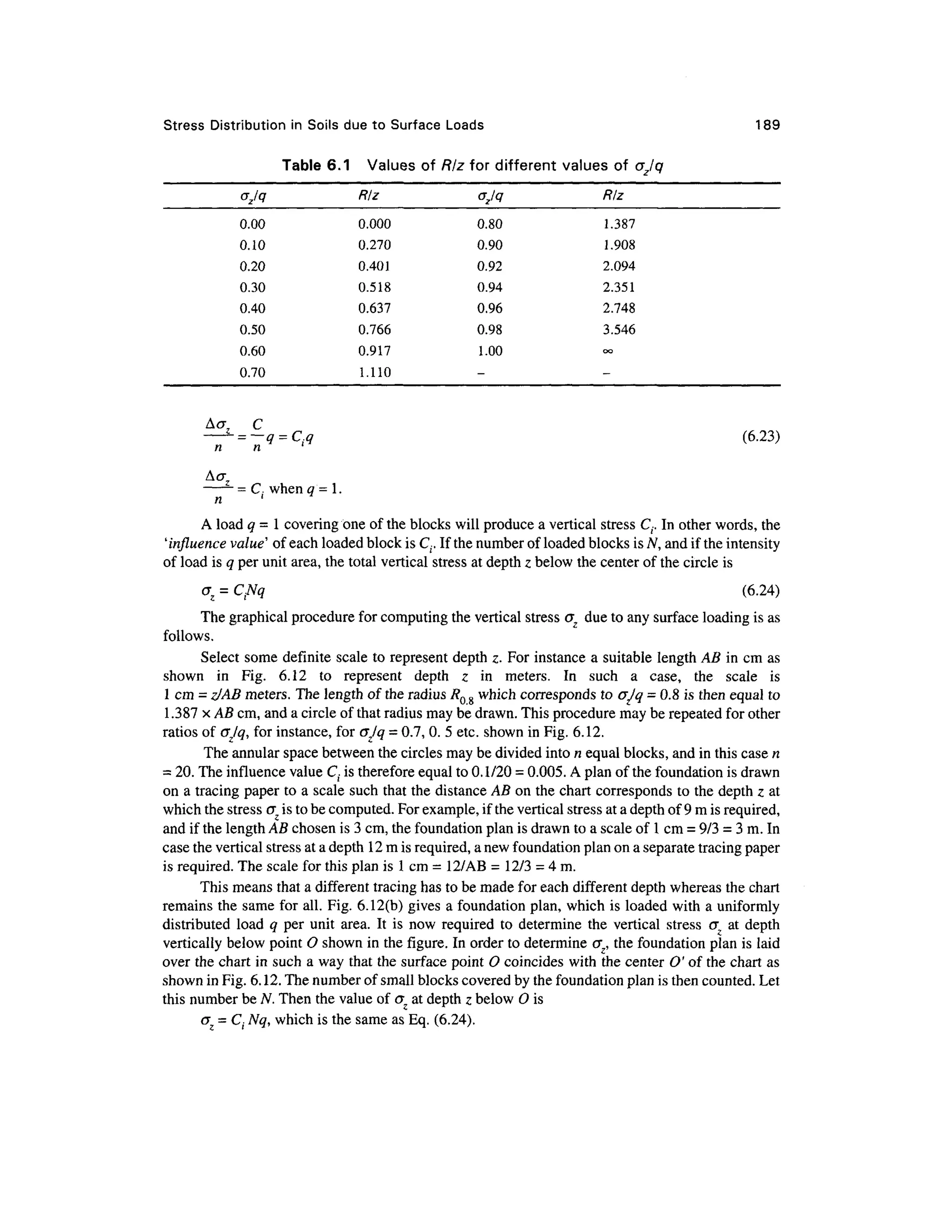
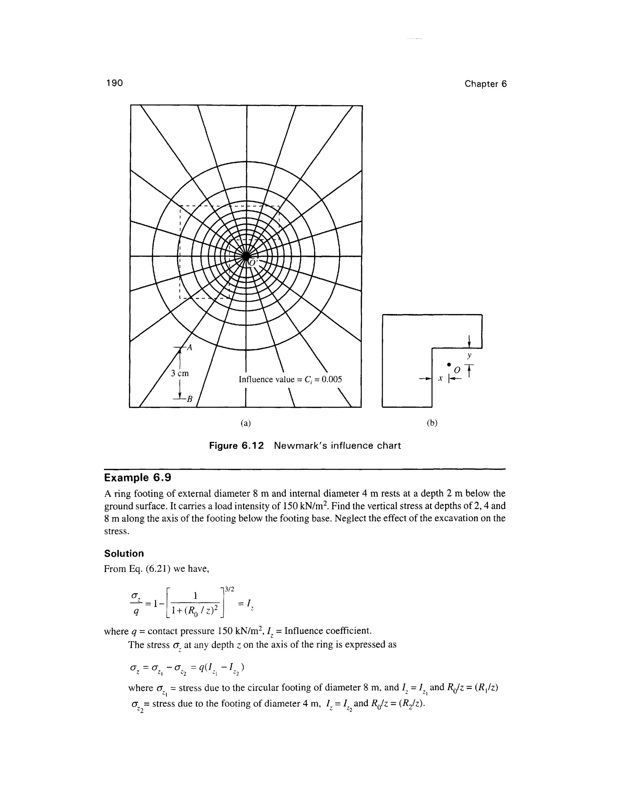
194. Stress Distributio n in Soils du e to Surfac e Loads 175
that I B ha s a maximu m valu e o f 0.4 8 a t r/ z = 0, i.e. , indicatin g thereb y tha t th e stres s i s a
maximum below th e point load .
6.3 WESTERGAARD' S FORMUL A FO R POINT LOAD S
Boussinesq assume d tha t the soil is elastic, isotropic an d homogeneous for the development o f a
point loa d formula . However, th e soil i s neither isotropic no r homogeneous. Th e mos t commo n
type of soils that are met in nature are the water deposited sedimentary soils. When the soil particles
are deposited i n water, typical clay strata usually have their lenses of coarser materials within them.
The soil s o f thi s typ e ca n b e assume d a s laterall y reinforce d b y numerous , closel y spaced ,
horizontal sheets of negligible thickness but of infinite rigidity, which prevent the mass as a whole
from undergoing lateral movement of soil grains. Westergaard, a British Scientist, proposed (1938 )
a formula for the computation of vertical stress oz b y a point load, Q, at the surface as
cr, -'
Q
,3/2 2 M (6.2)
in whichfj, i s Poisson's ratio. Iffj, i s taken as zero for all practical purposes, Eq . (6.2) simplifies t o
Q 1 Q
[l +2(r/z)2
]3
'2 (6.3)
where /,, , =
(II a)
[l + 2(r/z)2
]3/2
is the Westergaard stres s coefficient . Th e variatio n o f / wit h the
ratios of (r/z) i s shown graphically in Fig. 6.2 along with the Boussinesq's coefficien t IB. The value
of Iw a t r/z = 0 is 0.32 which is less than that of IB by 33 per cent.
h or 7
w
0 0. 1 0. 2 0. 3 0. 4 0. 5
r/z 1. 5
2.5
Figure 6.2 Value s of IB or /^for use in the Boussines q o r Westergaard formul a

195. 176 Chapter s
Geotechnical engineer s prefe r t o us e Boussinesq' s solutio n a s thi s give s conservativ e
results. Further discussions ar e therefore limited to Boussinesq's metho d i n this chapter.
Example 6. 1
A concentrated load of 100 0 kN is applied at the ground surface. Compute the vertical pressure (i)
at a depth o f 4 m belo w th e load , (ii) at a distance of 3 m a t th e sam e depth . Use Boussinesq' s
equation.
Solution
The equation is
Q 3/2; r
_ _ —/ wher e /„ = rrj^-
Z 7 i if ' t i f 9 p/Z
z
[l + ( r / z ) 2
Q 100 0
(i) When r/ z = 0, /„ = 3/2 n = 0.48, a = 0.48^
- = 0.48 x —— = 30 kN/m2
B z
z 2
4x 4
(ii) When r/ z = 3/4 = 0.75
3/27T 0.156x100 0
I
R=~T ^ T = 0.156, a = — = 9.8 kN/m2
B
l + (0.75)2
f2 z 4 x 4
Example 6. 2
A concentrated load of 45000 Ib acts at foundation level at a depth of 6.56 ft below ground surface .
Find th e vertica l stress alon g the axis of the load a t a depth o f 32.8 f t and a t a radial distanc e of
16.4 ft at the same dept h by (a) Boussinesq, and (b) Westergaard formula e for n = 0. Neglect th e
depth of the foundation .
Solution
(a) Boussinesq Eq. (6.la)
"2
z
z 2 B
' B
271 l + ( r / z ) 2
Substituting the known values, and simplifyin g
IB = 0.2733 for r/ z = 0.5
= _45000x02733^n431b/ft2
z
(32.8) 2
(b) Westergaard (Eq . 6.3 )
13/2
Q 1
l + 2(r/z)2
Substituting the known values and simplifying, w e have,
/ = 0.1733forr/ 7 = 0.5

196. Stress Distribution in Soils due to Surfac e Load s 177
therefore,
a =
(32.8)
x 0.1733 =7.25 lb/ft2
Example 6. 3
A rectangular raf t o f siz e 3 0 x 1 2 m founded at a depth o f 2. 5 m below th e groun d surfac e is
subjected t o a unifor m pressur e o f 15 0 kPa . Assum e th e cente r o f th e are a i s th e origi n o f
coordinates (0 , 0). and the corners have coordinates (6 , 15) . Calculate stresses at a depth of 20 m
below the foundation level by the methods of (a) Boussinesq, and (b) Westergaard at coordinates of
(0, 0), (0, 15), (6, 0) (6, 15) and (10, 25). Also determine the ratios of the stresses as obtained by the
two methods. Neglect the effect o f foundation depth on the stresses (Fig. Ex. 6.3) .
Solution
Equations (a) Boussinesq:
(b) Westergaard:
= — I B,
z
IB = '
l + <r/^f2
Q 0.32
The ratios of r/z at the given locations for z = 20 m are as follows:
Location
(0,0)
(6,0)
(0, 15)
r/z
0
6/20 = 0.3
15/20 = 0.75
Location
(6, 15 )
(10, 25)
(^
(Vio2
"
r/z
f 152
)/20 = 0.81
+ 252
)/20 = 1.35
The stresse s at the various locations at z = 20 m may be calculated by using the equations given
above. The results are tabulated below for the given total load Q = qBL = 150 x 12 x 30 = 54000 kN
acting at (0, 0) coordinate. Q/z 2
=135.
(6,15) (6,0) (6,15)
.(0,0) (0,15)
(6,15) (6,0)
Figure Ex. 6. 3
(6,15)
(10,25)

197. 178 Chapter 6
Location r/ z Boussinesq
I0 crJkPa )
Westergaard
w
a/a, w
(0,0)
(6,0)
(0, 15 )
(6,15)
(10, 25 )
0
0.3
0.75
0.81
1.35
0.48
0.39
0.16
0.14
0.036
65
53
22
19
5
0.32
0.25
0.10
0.09
0.03
43
34
14
12
4
1.51
1.56
1.57
1.58
1.25
6.4 LIN E LOAD S
The basi c equatio n use d fo r computin g a, at an y poin t P i n a n elasti c semi-infinit e mass i s
Eq. (6.1) of Boussinesq. By applyin g the principle of his theory, the stresse s a t any poin t in the
mass due to a line load of infinite extent acting at the surface may be obtained. The state of stress
encountered i n thi s cas e i s tha t o f a plan e strai n condition . Th e strai n a t an y poin t P i n th e
F-direction parallel to the line load is assumed equal to zero. The stress c r norma l to the XZ-plane
(Fig. 6.3) is the same at all sections and the shear stresses o n these sections ar e zero. By applying
the theor y o f elasticity , stresse s a t an y poin t P (Fig . 6.3 ) ma y b e obtaine d eithe r i n pola r
coordinates o r i n rectangula r coordinates. Th e vertica l stres s a a t poin t P ma y b e writte n in
rectangular coordinate s a s
a =
z [ 1 + U/z)2
]2
z z
where, / i s the influence factor equal to 0.637 at x/z - 0 .
(6.4)
r — i x•" • + z
cos fc) =
Figure 6.3 Stresse s due to vertica l lin e loa d i n rectangular coordinate s

198. Stress Distributio n in Soils du e to Surfac e Load s 179
6.5 STRI P LOAD S
The state of stress encountered i n this case also is that of a plane strain condition. Suc h conditions
are found fo r structures extended ver y much in one direction, suc h as strip and wall foundations,
foundations of retaining walls, embankments, dams and the like. For such structures the distribution
of stresses in any section (except for the end portions of 2 to 3 times the widths of the structures from
its end) will be the same as in the neighboring sections, provided that the load does no t change in
directions perpendicular to the plane considered.
Fig. 6.4(a ) shows a load q per unit area acting on a strip of infinite lengt h and of constant
width B. The vertical stress at any arbitrary point P due to a line load of qdx actin g at j c = x can be
written from Eq . (6.4) as
~
2q
n [(x-x) 2
+z2
]
(6.5)
Applying th e principl e o f superposition , th e tota l stres so~ z a t poin t P du e t o a stri p loa d
distributed over a width B(= 2b) may be written as
+b
[(x-x)2
+z2
}2 dx
or
-b
q , z
a = — tan" 1
1
n x-b
tan"
2bz(x2
-b2
-z2
)
x + b (6.6)
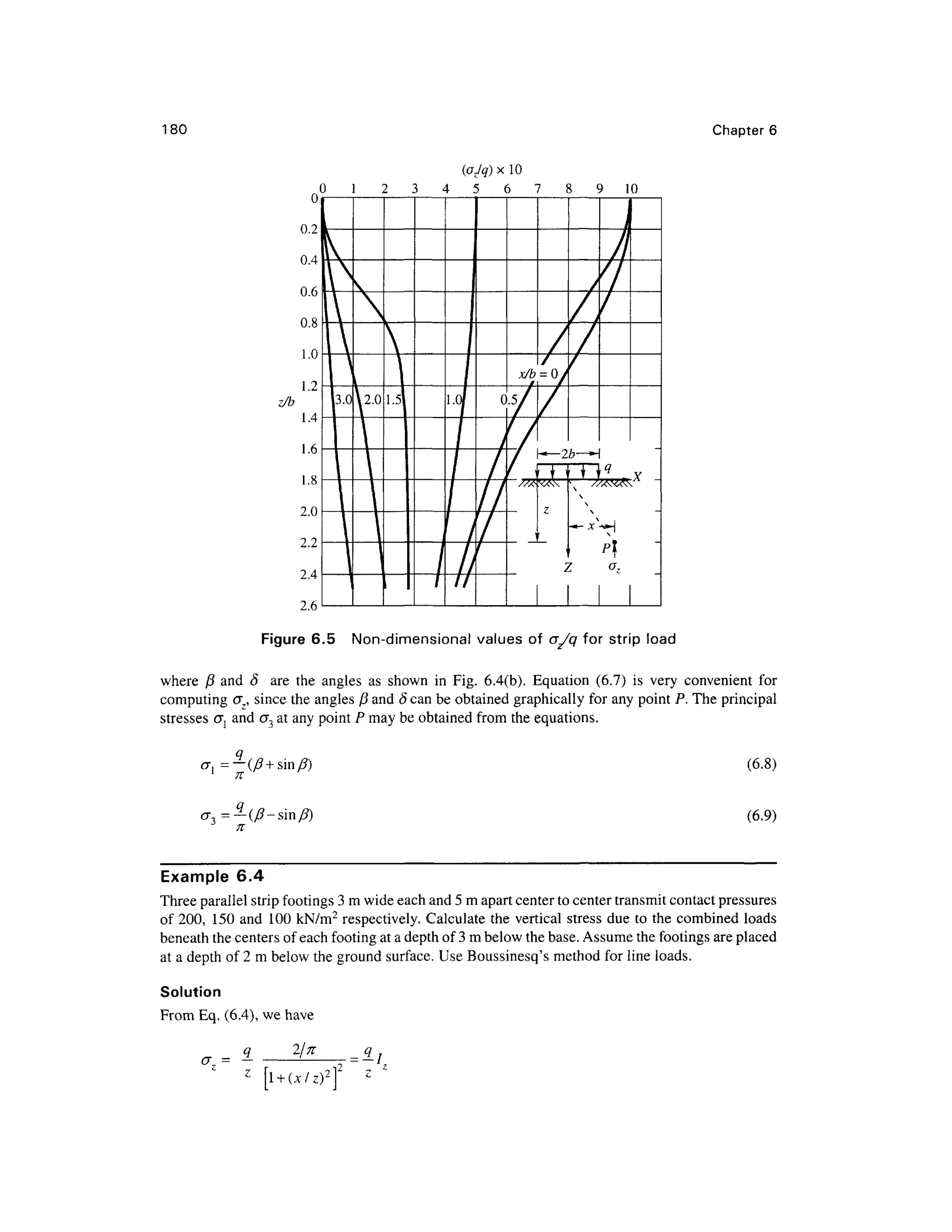
The non-dimensiona l value s o f cjjq ar e give n graphicall y i n Fig. 6.5 . Eq. (6.6 ) can b e
expressed i n a more convenient form as
=— [/?+sin/?cos(/?+2£)]
n
(6.7)
x O
(a) (b )
Figure 6.4 Stri p load

199. 180 Chapter 6
(ajq) x 1 0
4 5 6 7 10
Figure 6.5 Non-dimensiona l value s of <j/q fo r stri p loa d
where / 8 and S ar e th e angle s a s show n i n Fig . 6.4(b) . Equatio n (6.7 ) i s ver y convenien t fo r
computing o~ , since the angles ft and S can be obtained graphically for any point P. The principal
stresses o { an do" 3 at any point P may be obtained from the equations.
cr, = —(/?+sin/?)
n
(6.8)
0", =— (p-sm,
TC
(6.9)
Example 6. 4
Three parallel strip footings 3 m wide each and 5 m apart center to center transmit contact pressure s
of 200 , 15 0 and 10 0 kN/m2
respectively. Calculate the vertica l stres s du e to the combined load s
beneath the centers of each footing at a depth of 3 m below the base. Assume the footings are placed
at a depth of 2 m below the ground surface. Use Boussinesq's method for line loads.
Solution
From Eq. (6.4), we have
2/;r _ q
_2

200. Stress Distributio n in Soils due to Surfac e Load s 181
XXXx
1
2
C „- .
30
1
1
c
50
1
loot
xxxxc
J^/m2
3m
,
3 m
t y
3 m
t
3 m
C
Figure Ex. 6.4 Thre e parallel footing s
The stress at A (Fig. Ex. 6.4) is
(4 =
2x200F 1
3.14x3
2x100
2x150
3.14x3
1
_l + (5/3)2
3.14x3_l + (10/3)2 = 45 kN/m2
The stress at B
("•}
z) B
2x200
3x
1
_l + (5/3)2
2x150
2x100
(0/3)
= 36.3 kN / m2
The stress at C
kt=
2x200
l + (10/3)2
2x150 1
3^r l + (5/3)2
2x100
= 23.74 kN/m2
6.6 STRESSE S BENEAT H THE CORNE R O F A RECTANGULAR
FOUNDATION
Consider an infinitely smal l unit of area of size db x dl, shown in Fig. 6.6. The pressure acting on
the small area may be replaced by a concentrated load dQ applied to the center of the area.
Hence
= qdb.dl (6.10)
The increase of the vertical stress a du e to the load dQ can be expressed per Eq. (6.11) as

201. 182 Chapter 6
* ^r
i:M
1
1 1
s
'
'
<1 '
'
N
'
'
Figure 6.6 Vertica l stress under th e corne r of a rectangular foundatio n
dcr =
dQ 3z 3
(6.11)
The stress produced by the pressure q over the entire rectangle b x I can then be obtained by
expressing dl, db and r in terms of the angles a and /3, and integrating
a=a} /?
= /? ,
(6.12)
There are several form s of solution for Eq . (6.12) . The one tha t is normally use d i s of the
following form
cr=q
or
2mn(m2
+n2
+1)1/2
m 2
+n2
+2
m2
+n2
+m2
n2
+l m 2
+n2
+l
tan
_, 2mn(m 2
+n2
+l)l/2
m2
+n2
-m2
n2
+1 (6.13)
az = ql (6.14 )
wherein, m = b/z, n = l/z,are pure numbers. / is a dimensionless factor and represents the influence
of a surcharge covering a rectangular area on the vertical stress at a point located at a depth z below
one of its corners .
Eq. (6.14) i s presented i n graphical form in Fig. 6.7. This chart helps to compute pressure s
beneath loaded rectangula r areas. The chart also shows that the vertical pressure i s not materially
altered if the length of the rectangle is greater than ten times its width. Fig. 6.8 may also be used for
computing the influence value / based on the values of m and n and may also be used to determine
stresses belo w points that lie either inside or outside the loaded area s as follows.

202. Stress Distributio n in Soils du e to Surfac e Loads 183
z/b =
0.05
Values of / = ojq
0.10 0.1 5 0.20 0.25
Figure 6.7 Char t fo r computin g G Z below th e corne r o f a rectangular foundatio n
(after Steinbrenner , 1934 )
When the Poin t i s Inside
Let O be an interior point of a rectangular loaded are a ABCD show n in Fig. 6.9(a) . I t is required
to compute the vertical stress<J z below this point O at a depth z from the surface. For this purpose,
divide the rectangle ABCD int o four rectangles marked 1 to 4 in the Fig. 6.9(a) by drawing lines
through O . For eac h o f thes e rectangles , comput e th e ratio s zfb. Th e influenc e valu e 7 may b e
obtained from Fig. 6.7 or 6.8 for each of these ratios and the total stress at P is therefore
_. / T . T . J . T / S I C
&7 = q Ui + h + M + y
J (6.15 )
When the Poin t i s Outside
Let O be an exterior point of loaded rectangular area ABCD shown in Fig. 6.9(b). It is required to
compute the vertical stress<T Z below point 0 a t a depth z from the surface.
Construct rectangles a s shown in the figure. The point O is the corner point of the rectangle
OBlCDr Fro m th e figure it can be seen that
Area ABCD = OB1CD1 - OB {BD2 - OD }DA{ + OA1AD2 (6.16 )

203. 184 Chapter 6
0.00
0.01 2 4 6 80. 1 2 4 6 81. 0
Values of n = l/z
4 6 8 10
Figure 6.8 Grap h for determinin g influenc e valu e for vertica l norma l stres s cr z at
point P located beneat h on e corner of a uniformly loade d rectangular area . (Afte r
Fadum, 1948 )
O
fb
I
1 2
^ 6
3 4
D C
(a) When the point 'O' is within the rectangle (b ) When the point 'O' is outside the rectangle
Figure 6.9 Computatio n o f vertical stress belo w a poin t

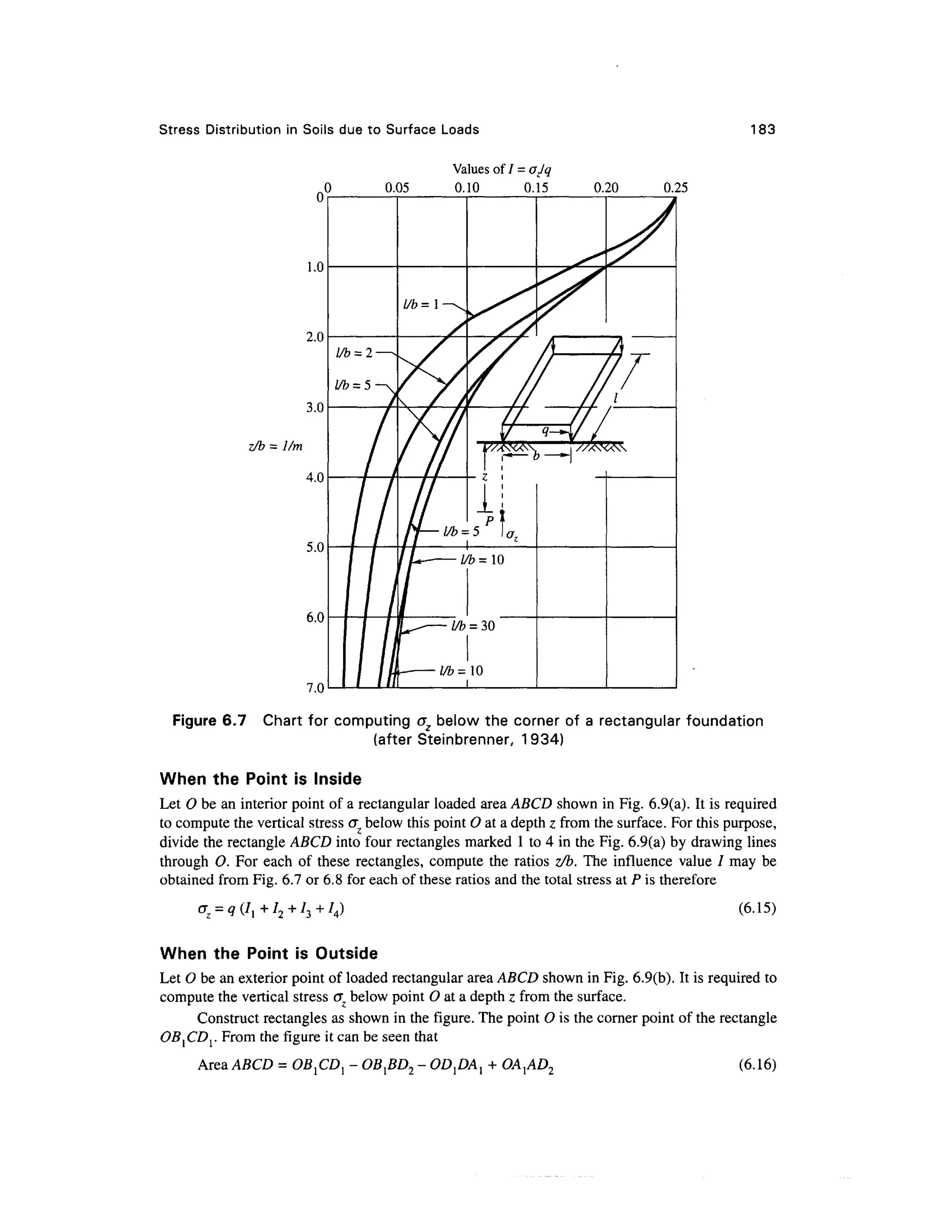
204. Stress Distribution in Soils due to Surfac e Load s 18 5
The vertical stress a t point P located a t a depth z below poin t 0 du e to a surcharge q per
unit are a o f ABCD i s equa l t o the algebrai c su m o f the vertica l stresse s produce d b y loadin g
each one of the areas liste d on the right hand side of the Eq. (6.16) with q per unit of area. If /j
to /4 are the influence factors of each of these areas, th e total vertica l stres s is
(6.17)
Example 6. 5
ABCD i s a raf t foundatio n o f a multi-stor y building [Fig . 6 . 9(b) ] wherei n AB = 65.6 ft , an d
BC = 39.6 ft. The uniformly distributed load q over the raft is 73 10 lb/ft2
. Determine crz at a depth of
19.7 ft below point O [Fig. 6.9(b)] wherein AA, = 13.12 ft and A,0 = 19.68 ft. Use Fig. 6.8 .
Solution
Rectangles are constructed as shown in [Fig. 6.9(b)].
Area ABCD = OB}CDl - OB }BD2 - OD 1DA1 + OA1AD2
Rectangle
OB1CD1
OB1BD2
OD1DA1
OA{AD2
I
(ft)
85.28
85.28
52.72
19.68
b
(ft)
52.72
13.12
19.68
13.12
m
2.67
0.67
1.00
0.67
n
4.33
4.33
2.67
1.00
7
0.245
0.168
0.194
0.145
Per Eq. (6.17)
oz = q (/! - /2 - /3 + /4) =7310 (0.24 5 - 0.168 - 0.194 + 0.145) = 204.67 lb/ft2
The same value can be obtained using Fig. 6.7 .
Example 6. 6
A rectangula r raf t o f siz e 3 0 x 1 2 m founde d on th e groun d surface i s subjecte d t o a uniform
pressure of 150 kN/m2
. Assume the center of the area as the origin of coordinates (0,0), and corners
with coordinates (6 , 15) . Calculate the induced stress a t a depth of 20 m by the exact method at
location (0, 0).
Solution
Divide the rectangle 1 2 x 30 m into four equal parts of size 6 x 15m.
The stres s belo w th e corne r o f eac h footin g ma y b e calculate d b y usin g chart s give n in
Fig. 6.7 or Fig. 6.8. Here Fig. 6.7 is used.
For a rectangle 6 x 1 5 m, z Ib = 20/6 = 3.34, l/b = 15/6 = 2.5.
For z/b = 3.34, l/b = 2.5,< r Iq = 0.07
Therefore, o ; = 4cr = 4 x 0.01 q= 4 x 0.07 x 15 0 =42 kN/m2
.

205. 186 Chapter 6
6.7 STRESSE S UNDE R UNIFORML Y LOADE D CIRCULA R FOOTIN G
Stresses Along the Vertica l Axis of Symmetry
Figure 6.1 0 show s a pla n an d sectio n o f th e loade d circula r footing . The stres s require d t o b e
determined a t any point P along the axis is the vertical stress cr,.
Let dA be an elementary area considered as shown in Fig. 6.10. dQ may be considered as the
point load acting on this area which is equal to q dA. We may write
(6.18)
The vertical stress d(J a t point P due to point load dQ may be expressed [Eq . (6. la)] as
3q
(6.19)
The integral form of the equation for the entire circular area may be written as
0=0 r= 0
3qz3
( f rdOdr
~^~ J J ( r 2 + z 2 ) 5 ,
0=0 r= 0
,3
On integration we have, (6.20)
o
R z
P
Figure 6.10 Vertica l stress unde r uniforml y loade d circular footin g

206. Stress Distributio n in Soils due to Surfac e Load s 187
Influence value 7Z (xlOO)
1.0 1 0
Note: Numbers on curves
indicate value of r/R Q
Figure 6.11 Influenc e diagra m for vertica l norma l stres s at various point s withi n
an elastic half-spac e under a uniformly loade d circula r area . (After Foste r and
Ahlvin, 1954 )
or
3/2
(6.21)
where, /. , i s th e Influence coefficient. Th e stres s a t an y poin t P o n th e axi s o f symmetr y o f a
circular loade d are a ma y b e calculate d b y th e us e o f Eq . (6.21 ) Vertica l stresse so ~ ma y b e
calculated by using the influence coefficient diagram given in Fig. 6.11.
Example 6. 7
A water tank is required to be constructed with a circular foundation having a diameter of 1 6 m
founded a t a dept h o f 2 m belo w th e groun d surface . Th e estimate d distribute d loa d o n th e
foundation i s 325 kN/m2
. Assuming that the subsoil extends to a great depth and is isotropic and
homogeneous, determine the stresses ot at points (i) z = 8 m, r = 0, (ii) z=8 m, r = 8 m, (iii) z= 16
m, r = 0 and (iv) z=16m, r = 8m, where r is the radial distance from the central axis. Neglect the
effect o f the depth of the foundation on the stresses. (Use Fig. 6.11)
Solution
q — 325 kN/m2
, RQ = 8 m. The results ar e given in a tabular form as follows :
(i)
(ii)
(iii)
(iv)
Point
(8,0)
(8,8)
(16,0)
(16, 8)
z//?0
1
1
2
2
r/HQ
0
1.0
0
1.0
/
0.7
0.33
0.3
0.2
crzkN/m2
227.5
107.25
97.5
65

207. 188 Chapter 6
Example 6. 8
For a raft of size 98.4 x 39.36 ft, compute the stress at 65.6 f t depth below the center of the raft by
assuming that the rectangle can be represented by an equivalent circle. The load intensity on the raft
is31331b/ft2
.
Solution
The radiu s o f a fictitiou s circula r footin g o f are a equa l t o th e rectangula r footin g o f siz e
98.4 x 39.36 ft is
= 98.4 x 39.36 = 3873 sq. ft o r RQ = p
= 35.12 ft
V
Use Eq. (6.21) for computing a a t 35.6 ft depth
65.6
35.12
Now, z/R Q = -^^= 1.9 , and r/RQ = 0. From Fig. 6.11, 7Z = 0.3
Therefore, c r = 0.3 q = 0.3 x 3133 = 940 lb/ft 2
.
6.8 VERTICA L STRES S BENEAT H LOADE D AREA S OF IRREGULAR
SHAPE
Newmark's Influenc e Chart
When the foundation consists of a large number of footings or when the loaded mats or rafts are not
regular i n shape , a char t develope d b y Newmar k (1942 ) i s mor e practica l tha n th e method s
explained before. It is based on the following procedure. The vertical stress cr , below the center of
a circular area of radius R which carries uniformly distributed load q is determined per Eq. (6.21).
It may be seen from Eq . (6.21) that when Rlz = °°,az/q=l, tha t is cr, = q. This indicates that
if the loaded area extends to infinity, the vertical stress in the semi-infinite solid at any depth z is the
same as unit load q at the surface. If the loaded area is limited to any given radius R it is possible to
determine from Eq . (6.21) the ratios Rlz for which the ratio of Gjq ma y have any specified value,
say 0.8 or 0.6. Table 6.1 gives the ratios of Rlz for different value s of <j/q.
Table 6.1 may be used for the computation of vertical stress<J 7 at any depth z below the center
of a circular loaded area of radius R. For example, at any depth z, the vertical stress o^ = 0.8 q if the
radius o f th e loade d are a a t the surfac e i s R = 1.387 z . At th e same depth , th e vertica l stres s is
cr = 0.7 q if R = 1.110 z. If instead of loading the whole area, if only the annular space between the
circles o f radii 1.38 7 z and 1.11 0 z are loaded, the vertical stress at z at the center of the circle is
ACT = 0. 8 q-0.7 q = 0.lq.Similarly if the annular space between circles of radii l.llO z and 0.91 7
z are loaded, th e vertical stress at the same depth z is ACT, = 0.7 q-0.6 q = 0.1 q. We may therefor e
draw a series of concentric circles on the surface of the ground in such a way that when the annular
space between an y two consecutive circles is loaded with a load q per unit area, the vertical stress
ACT produce d a t an y dept h z belo w th e cente r remains a constant fraction o f q . W e ma y write ,
therefore,
Aaz = Cq (6.22 )
where C is constant. I f an annular space between an y two consecutive concentri c circles is divided
into n equal blocks and if any one such block is loaded with a distributed load q, the vertical stress
produced a t the center is, therefore,

208. Stress Distribution in Soils due to Surfac e Load s 18 9
Table 6.1 Value s of Rlz for differen t value s of a' Iq
AaL
n
ajq
0.00
0.10
0.20
0.30
0.40
0.50
0.60
0.70
C
n '
Rlz
0.000
0.270
0.401
0.518
0.637
0.766
0.917
1.110
<V<7
0.80
0.90
0.92
0.94
0.96
0.98
1.00
-
Rlz
1.387
1.908
2.094
2.351
2.748
3.546
oo
-
(6.23)
z
-= C when< 7 = l.
nl
A load q = 1 covering one of the blocks will produce a vertical stress C- . In other words, the
'influence value' o f each loaded block is C(. If the number of loaded blocks is N, and if the intensity
of load is q per unit area, the total vertical stress at depth z below the center of the circle is
ot = CNq (6.24 )
The graphical procedure for computing the vertical stress GZ du e to any surface loading is as
follows.
Select som e definit e scale to represent dept h z. For instance a suitable length AB in cm as
shown i n Fig . 6.1 2 t o represen t dept h z i n meters . I n suc h a case , th e scal e i s
1 cm = zlAB meters. The length of the radius RQ g which corresponds to ajq = 0.8 is then equal to
1.387 x AB cm, and a circle of that radius may be drawn. This procedure may be repeated for other
ratios of ajq, for instance, for ojq = 0.7, 0. 5 etc. shown in Fig. 6.12.
The annular space between the circles may be divided into n equal blocks, and in this case n
= 20. The influence value C. is therefore equal to 0.1/20 = 0.005. A plan of the foundation is drawn
on a tracing paper t o a scale suc h that the distance AB on the chart corresponds t o the depth z at
which the stress c? z is to be computed. For example, if the vertical stress at a depth of 9 m is required,
and if the length AB chosen is 3 cm, the foundation plan is drawn to a scale of 1 cm = 9/3 = 3 m. In
case the vertical stress at a depth 12 mis required, a new foundation plan on a separate tracing paper
is required. The scale for this plan is 1 cm = 12/AB = 12/3 = 4 m.
This means that a different tracin g has to be made for each different dept h whereas the chart
remains the same for all. Fig. 6.12(b) gives a foundation plan, which is loaded wit h a uniformly
distributed loa d q pe r uni t area. I t i s no w require d t o determin e th e vertica l stres s & z a t depth
vertically below point O shown in the figure. In order to determine cr z, the foundation plan is laid
over the chart in such a way that the surface point O coincides wit h the center O' of the chart as
shown in Fig. 6.12. The number of small blocks covered by the foundation plan is then counted. Let
this number be N. Then the value of G Z at depth z below O is
az = Ci Nq, which is the same as Eq. (6.24).

209. 190 Chapter 6
Influence value = C. = 0.005
(a) (b )
Figure 6.12 Newmark' s influenc e char t
Example 6. 9
A ring footing o f external diamete r 8 m and internal diamete r 4 m rests at a depth 2 m below the
ground surface. It carries a load intensity of 150 kN/m2
. Find the vertical stress at depths of 2,4 and
8 m along the axis of the footing below the footing base. Neglect the effect of the excavation on the
stress.
Solution
From Eq . (6.21) we have,
1
3/2
where q = contact pressure 15 0 kN/m2
, /., = Influence coefficient.
The stres s o_ at any depth z on the axis of the ring is expressed a s
o; = cr. -U, = q(I, - /, )
Z ^ i <- 2 - i <-2
where cr , = stress due to the circular footing of diameter 8 m, and /, = I7 an d RQ/z =
cr = stress due to the footing of diameter 4m, / , = / an d RJz = (RJz).

210. Stress Distributio n in Soils due to Surfac e Load s 191
The values of /., may be obtained from Tabl e 6.1 for various values of /?0/z. The stress c r a t
depths 2, 4 and 8 m are given below:
Depth (m ) R^lz
2 2
4 1. 0
8 0. 5
'*,
0.911
0.647
0.285
R2/z l z
1.0 0.69 7
0.5 0.28 5
0.25 0.08 7
(/ - I 2 ) q = a z kN/m2
39.6
54.3
29.7
Example 6.1 0
A raf t foundatio n o f th e siz e give n i n Fig . Ex . 6.1 0 carrie s a uniforml y distribute d loa d o f
300 kN/m2
. Estimate the vertical pressure at a depth 9 m below the point O marked in the figure.
Solution
The depth at which &z required is 9 m.
Using Fig. 6.12 , th e scale o f the foundation plan is AB = 3 cm = 9 m or 1 cm = 3 m. The
foundation pla n is required t o be made t o a scale o f 1 cm = 3 m on tracing paper. Thi s plan is
superimposed o n Fig. 6.1 2 with O coinciding with the center o f the chart. The plan is shown in
dotted lines in Fig. 6.12.
Number of loaded blocks occupied by the plan, N = 62
Influence value, Cf = 0.005, q = 300 kN/m2
The vertical stress, cr z = C{ Nq - 0.00 5 x 62 x 300 = 93 kN/m2
.
18m-
16.5 m
3m
= x
6 m
1
3 m =
O
[•— 9m —-|
Figure Ex. 6.10
6.9 EMBANKMEN T LOADING S
Long earth embankments with sloping sides represent trapezoidal loads. When the top width of the
embankment reduces t o zero, th e load becomes a triangular strip load. The basi c proble m i s to
determine stresses due to a linearly increasing vertical loading on the surface.

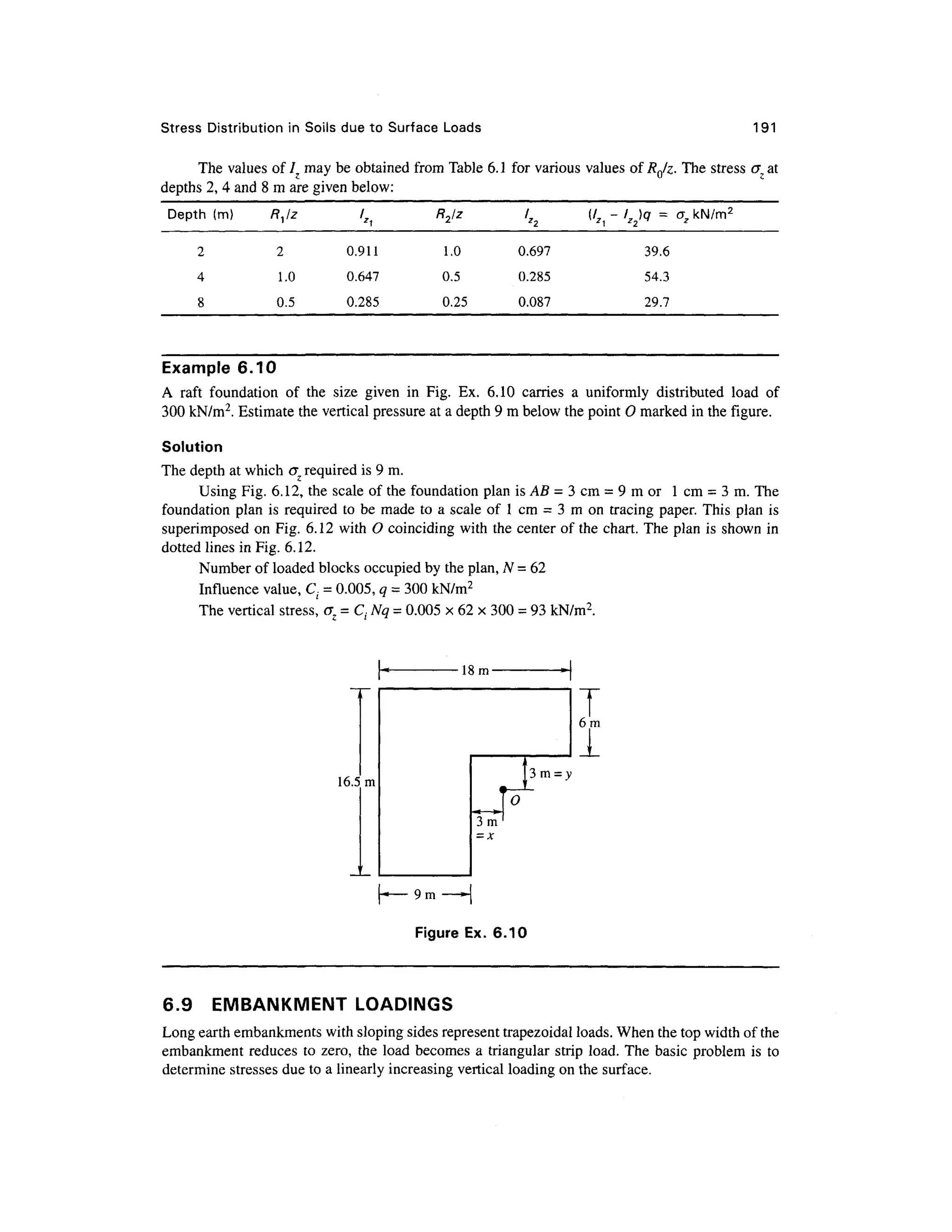
211. 192 Chapter s
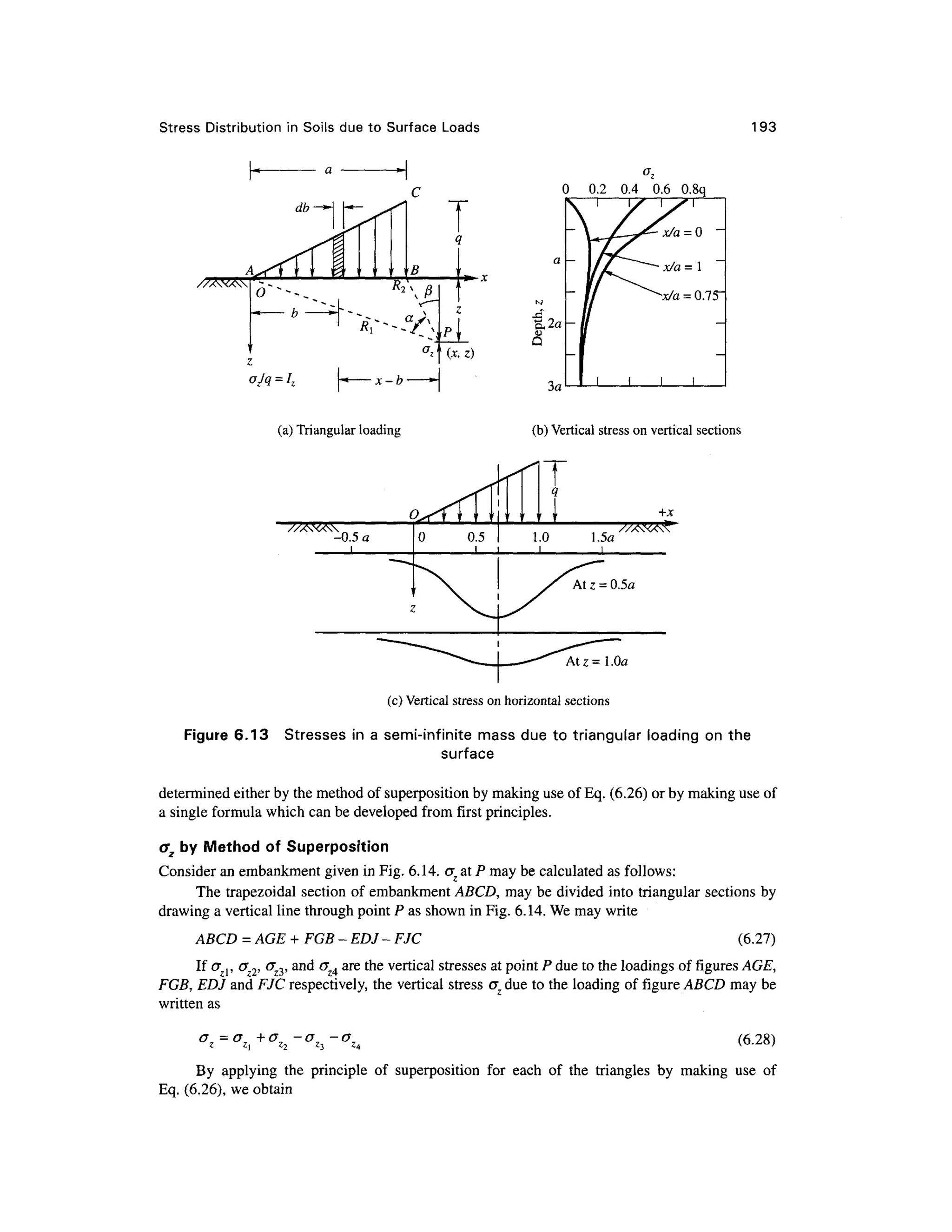
Linearly Increasin g Vertical Loadin g
Fig. 6.13(a ) shows a linearly increasing vertica l loadin g startin g fro m zero at A to a finite value q
per unit length at B. Consider a n elementary stri p of width db at a distance b from A. The load per
unit length may be written as
dq - (q/d) b db
Ifdq i s considered a s a line load on the surface, th e vertica l stres s dcr, at P [Fig . 6 . 1 3(a)]
due t o d q ma y b e writte n fro m Eq . (6.4 ) a s
dcr,=— —
'
Therefore,
er
b=a
2q
[(x-,
/ 9
on integration, o - = 77" ~~ a-sm20 = 07 (6.25 )
z
2/T a y z
where 7 i s non-dimensional coefficien t whose value s for various values of xla and zla are given in
Table 6.2 .
If th e point P lies in the plane BC [Fig. 6.13(a)], then j 8 = 0 at jc = a. Eq. (6.25) reduces to
vz=-(a) (6.26 )
<• n
Figs. 6.13(b ) an d (c ) sho w th e distributio n of stres s e r o n vertica l an d horizonta l section s
under th e actio n o f a triangular loadin g a s a function of q. The maximu m vertica l stres s occur s
below th e center of gravity of the triangular load as shown in Fig. 6.13(c) .
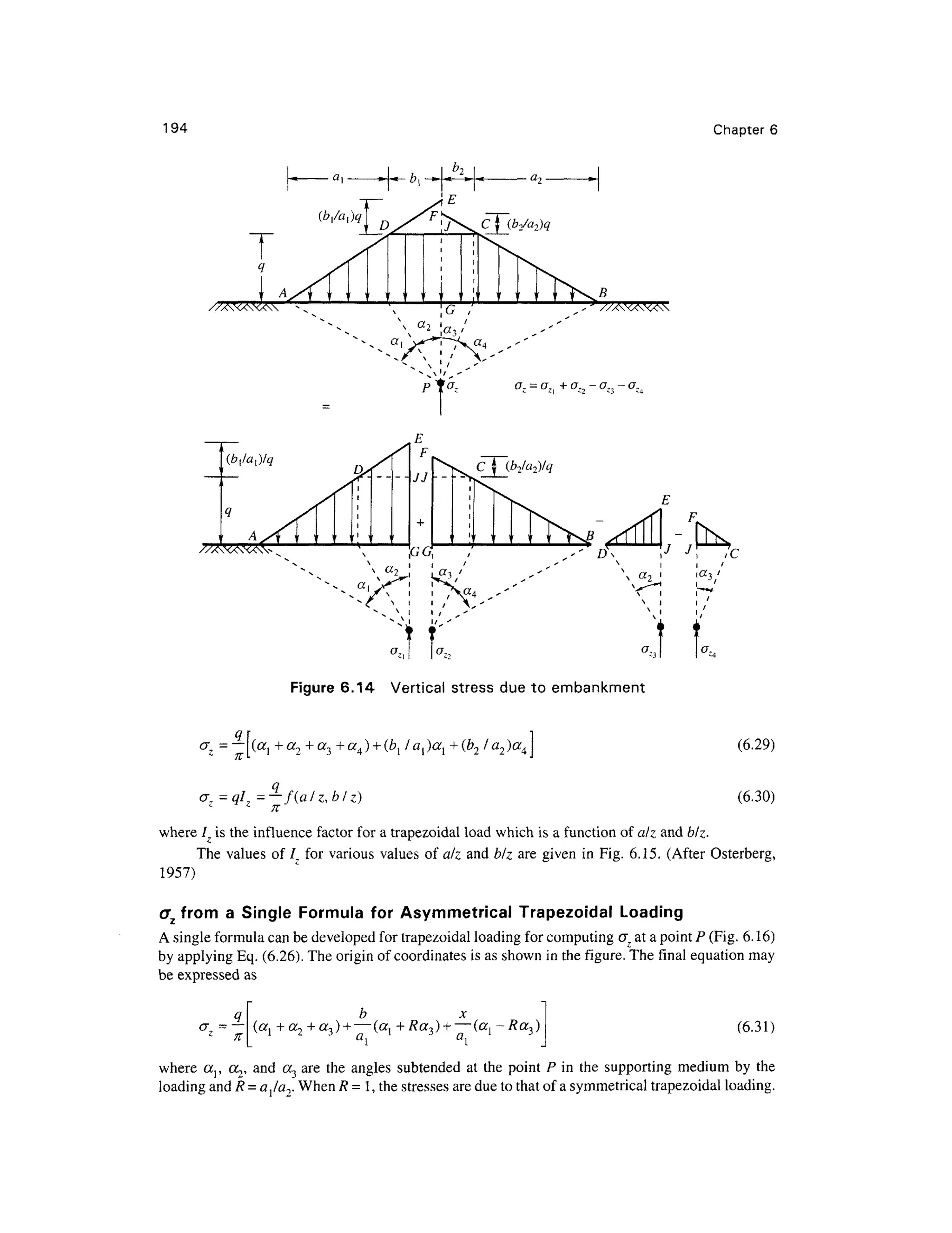
Vertical Stres s Du e to Embankmen t Loadin g
Many time s i t ma y b e necessar y t o determin e th e vertica l stres s e r beneat h roa d an d railwa y
embankments, an d als o beneat h eart h dams . Th e vertica l stres s beneat h embankment s ma y b e
Table 6. 2 / fo r triangula r loa d (Eq . 6.25 )
x/a
-1.500
-1.00
0.00
0.50
0.75
1.00
1.50
2.00
2.50
0.00
0.00
0.00
0.00
0.50
0.75
0.50
0.00
0.00
0.00
0.5
0.002
0.003
0.127
0.410
0.477
0.353
0.056
0.017
0.003
1.0
0.014
0.025
0.159
0.275
0.279
0.241
0.129
0.045
0.013
2/fl
1.5
0.020
0.048
0.145
0.200
0.202
0.185
0.124
0.062
0.041
2
0.033
0.061
0.127
0.155
0.163
0.153
0.108
0.069
0.050
4
0.051
0.060
0.075
0.085
0.082
0.075
0.073
0.060
0.049
6
0.041
0.041
0.051
0.053
0.053
0.053
0.050
0.050
0.045

212. Stress Distribution in Soils due to Surfac e Loads 193
0 0. 2 0. 4 0. 6 O. i
3a
(a) Triangular loading (b) Vertical stress on vertical section s
Atz= l.Of l
(c) Vertical stress on horizontal sections
Figure 6.1 3 Stresse s in a semi-infinite mas s due to triangula r loadin g o n the
surface
determined either by the method of superposition by making use of Eq. (6.26) or by making use of
a single formula which can be developed fro m first principles .
crz by Metho d o f Superposition
Consider an embankment given in Fig. 6.14. a at P may be calculated as follows:
The trapezoidal sectio n of embankment ABCD, may be divided into triangular sections by
drawing a vertical line through point P as shown in Fig. 6.14. We may write
ABCD = AGE +FGB-EDJ - FJC (6.27)
If < r r<T z2, Gzy and <7z4 are the vertical stresses at point P due to the loadings of figures AGE,
FGB, EDJ an d FJC respectively, the vertical stresso" z due to the loading of figure ABCD ma y be
written as
o=o -o - o
Z2
Z
3 Z (6.28)
By applyin g th e principl e o f superpositio n fo r eac h o f th e triangle s b y makin g us e o f
Eq. (6.26), w e obtain

213. 194 Chapter 6
//VCVC<XXV GG D X
0,.
Figure 6.14 Vertica l stres s due to embankmen t
K
(6.29)
a=ql=-f(a/z,b/z) (6.30)
where / is the influence factor for a trapezoidal load which is a function of a/z and biz.
The value s of /, for variou s values of a/z an d biz ar e given in Fig. 6.15. (After Osterberg ,
1957)
a^ from a Single Formul a fo r Asymmetrica l Trapezoida l Loadin g
A single formula can be developed for trapezoidal loading for computing CTZ a
t a point P (Fig. 6.16)
by applying Eq. (6.26). The origin of coordinates is as shown in the figure. The final equation may
be expressed as
(a, (a, +
X
— («!
a
i
(6.31)
where ar a 2, and «3 are the angles subtende d a t the point P in the supporting medium by the
loading and R = a,/a^.When R = 1, the stresses are due to that of a symmetrical trapezoidal loading.

214. Stress Distribution in Soils due to Surfac e Loads 195
0.50
0.40
0.30
0.20
0.10
0.01 2 4 6 8 0.1 2 4 6 8 1.0 2 4 6 8 1 0
Figure 6.15 A grap h to determin e compressiv e stresses from a load varying by
straight lin e law (Afte r Osterberg, 1957)
b b
a2—^
Figure 6.16 Trapezoida l loads

215. 196 Chapter 6
When the top width is zero, i.e, when b = 0, a2 = 0, the vertical stress < r wil l be due to a triangular
loading. The expression for triangular loading is
(6.32)
Eq. (6.31) and Eq. (6.32) can be used to compute c r a t any point in the supporting medium.
The angle s a {, cc 2, and a3 may conveniently be obtained b y a graphical procedur e wher e thes e
angles are expressed as radians in the equations.
Example 6.1 1
A 3 m high embankment is to be constructed a s shown in Fig. Ex . 6. 11. If the unit weight of soil
used in the embankment is 19.0 kN/m3
, calculate the vertical stress due to the embankment loading
at points PI; P2, and Py
M
3.0
F y= 19 kN/m
f
'3.0
i
Note: All dimensions ar e in metre s
P2 P^
Figure Ex. 6.11 Vertica l stresse s at Pv P2 &
Solution
q = yH = 19 x 3 = 57 kN/m2
, z = 3 m
The embankment is divided into blocks as shown in Fig. Ex. 6.11 for making use of the graph
given in Fig. 6. 15. The calculations are arranged a s follows:
Point
p{
P2
PI
Block
ACEF
EDBF
AGH
GKDB
HKC
MLDB
MACL
b
(m)
1.5
4.5
0
7.5
0
10.5
1.5
a
(m)
3
3
1.5
3
1.5
3.0
3.0
biz
0.5
1.5
0
2.5
0
3.5
0.5
alz
1
1
0.5
1.0
0.5
1.0
1.0
'
0.39
0.477
0.15
0.493
0.15
0.498
0.39

216. Stress Distributio n in Soils due to Surfac e Loads 197
Vertical stress<J z
At point P, , cr ,=
At point P 2,CF .
=
At point P y & z
=
(0.39 + 0.477) x 57 = 49.4 kN/m2
0. 15 x(57/2) + 0.493 x 57 -0.1 5 x (57/2) = 28.
(0.498 - 0.39) 57 =6.2 kN/m2
1 kN/m2
6.10 APPROXIMAT E METHODS FOR COMPUTING o 2
Two approximate methods are generally used for computing stresses i n a soil mass below loaded
areas. They are
1. Us e of the point load formulas such as Boussinesq's equation.
2. 2 : 1 method which gives an average vertical stress <r a t any depth z. This method assumes
that th e stresse s distribut e from th e loade d edg e point s a t an angl e o f 2 (vertical) to 1
(horizontal)
The first method if properly applied gives the point stress at any depth which compares fairly
well wit h exact methods , wherea s th e secon d doe s no t giv e any point stres s but onl y gives a n
average stress cr at any depth. The average stress computed by the second method has been foun d
to be in error depending upon the depth at which the stress is required.
Point Loa d Metho d
Eq. (6.1) may be used for the computation of stresses in a soil mass due to point loads acting at the
surface. Since loads occupy finite areas, the point load formula may still be used if the footings are
divided int o smaller rectangles o r square s and a series o f concentrated load s o f valu e q dA ar e
assumed to act at the center of each square or rectangle. Here dA is the area of the smaller blocks
and q the pressure per unit area. The only principle to be followed in dividing a bigger area into
smaller blocks is that the width of the smaller block should be less than one-third the depth z of the
point at which the stress is required to be computed. The loads acting at the centers of each smaller
area ma y b e considere d a s poin t load s an d Boussinesq' s formul a ma y the n b e applied . Th e
difference betwee n th e point load metho d an d the exact metho d explaine d earlie r i s clear fro m
z/B
Figure 6.17 c r b y point load method

217. 198 Chapter 6
Figure 6.18 c r 2 : 1 method
Fig. 6.17. In this figure th e absciss a o f the curve Cl represent s th e vertica l stress(7. , at differen t
depths z below the center of a square area B x B which carries a surcharge g per unit area or a total
surcharge load of B2
q. This curve is obtained by the exact method explained under Sect. 6.6. The
abscissa o f the curve C2 represents the corresponding stresses du e to a concentrated load Q = B2
q
acting at the center of the square area. The figure shows that the difference between the two curves
becomes ver y small fo r value s of z/B i n excess o f three. Henc e i n a computation of the vertica l
stress cr, at a depth z below an area, the area should be divided into convenient squares or rectangles
such that the least width of any block is not greater than z/3.
2 : 1 Metho d
In thi s method , th e stres s i s assume d t o b e distribute d uniforml y ove r area s lyin g below th e
foundation. The size of the area at any depth is obtained by assuming that the stresses spread out at
an angle of 2 (vertical) to 1 (horizontal) from the edges of the loaded areas shown in Fig. 6.18. The
average stress at any depth z is
Q
(B+z)(L
(6.33)
The maximu m stres s o m by a n exact metho d belo w th e loade d are a i s differen t fro m th e
average stress a a t the same depth. The value of cr/tr reache s a maximum of about 1. 6 at zlb =
0-5, where b = half width.
6.11 PRESSUR E ISOBAR S
Definition
An isobar i s a line which connects al l points of equal stress below th e ground surface . In other
words, an isobar is a stress contour. We may draw any number of isobars as shown in Fig. 6.19 for
any given load system . Each isobar represents a fraction o f the load applied a t the surface. Since
these isobar s for m closed figure s and resemble th e form of a bulb, they are als o termed bulb of
pressure or simply the pressure bulb. Normally isobars are drawn for vertical, horizontal and shear
stresses. The one that is most important in the calculation of settlements of footings is the vertical
pressure isobar .

218. Stress Distributio n in Soils due to Surfac e Loads 199
Lines of
equal vertical
pressure or
isobars
Figure 6.19 Bul b o f pressure
Significant Dept h
In hi s openin g discussio n o n
settlement o f structure s a t th e
First Internationa l Conferenc e
on Soi l Mechanic s an d
Foundation Engineering (held in
1936 a t Harvar d Universit y i n
Cambridge, Mass , USA) ,
Terzaghi stresse d th e
importance o f th e bul b o f
pressure an d it s relationshi p
with th e sea t o f settlement . As
stated earlie r w e may dra w any
number of isobars fo r any given
load system , but the on e tha t is
of practica l significanc e i s th e
one which encloses a soil mass which is responsible for the settlement of the structure. The depth of
this stressed zone may be termed as the significant depth DS which is responsible for the settlement
of the structure. Terzaghi recommended that for all practical purposes one can take a stress contour
which represents 20 per cent of the foundation contact pressure q, i.e, equal to Q.2q. The depth of
such an isobar can be taken as the significant depth Ds which represents the seat of settlement for
the foundation. Terzaghi's recommendation wa s based o n his observation that direct stresse s are
considered o f negligible magnitude when they are smaller than 20 per cent of the intensity of the
applied stress from structural loading, and that most of the settlement, approximately 80 per cent of
the total, takes place at a depth less than Ds. The depth Ds is approximately equal to 1. 5 times the
width of square or circular footings [Fig. 6.20(a)].
If several loaded footing s are spaced closely enough, the individual isobars of each footing
in questio n woul d combin e an d merg e int o on e larg e isoba r o f the_intensit y a s show n i n
[Fig. 6.20(b)]. The combined significan t dept h D i s equal to about 1. 5 B .
az = Q.2q
D<=.5B Stresse d zone
Isobar
(a) Significant depth of stressed zone
for single footing
Isobar
Combined stressed zone
(b) Effect o f closely placed footings
Figure 6.2 0 Significan t dept h o f stressed zon e

219. 200 Chapter 6
Pressure Isobar s for Footings
Pressure isobar s o f square , rectangula r an d circula r footing s ma y convenientl y b e use d fo r
determining vertical pressure, (J z, a t any depth, z, below the base of the footings. The depths z from
the groun d surface , an d th e distanc e r (o r jc ) fro m th e cente r o f th e footin g ar e expresse d a s a
function o f the width of the footing B. In the case of circular footing B represents th e diameter.
The followin g pressur e isobar s ar e give n base d o n eithe r Boussines q o r Westergaard' s
equations
1. Boussines q isobars for square and continuous footings, Fig. 6.21.
2. Boussines q isobar for circular footings, Fig. 6.22.
3. Westergaar d isobar s for square and continuous footings, Fig. 6.23 .
B/2=b BI2
= b
Continuous
25
Figure 6.2 1 Pressur e isobar s base d on Boussines q equatio n for squar e an d
continuous footings

220. Stress Distribution in Soils du e to Surfac e Loads 201
Figure 6.22 Pressur e isobars base d on Boussinesq equatio n fo r uniforml y loade d
circular footing s
B/2=b B/2
= b
5b
6b
Continuous
IB 2 B 3 5
Figure 6.23 Pressur e isobars based on Westergaard equatio n for squar e and
continuous footing

221. 202 Chapter 6
Example 6.1 2
A singl e concentrate d loa d o f 100 0 kN act s a t th e groun d surface . Construc t a n isoba r fo r
<7 = 40 kN/m2
by making use of the Boussinesq equation.
Solution
From Eq. (6.la) we have
3(2 1
We may now write by rearranging an equation for the radial distance r as
-1
Now for Q = 1000 kN, cr , = 40 kN/m2
, we obtain the values of rp r 2, ry etc . for differen t
depths z,, z2, zv etc. The values so obtained are
z(m)
0.25
0.50
1.0
2.0
3.0
3.455
r(m)
1.34
1.36
1.30
1.04
0.60
0.00
g=1000kN
a, = 40 kN/mJ
Isobar
3.455
Figure Ex . 6.12

222. Stress Distributio n in Soils due to Surfac e Load s 203
The isoba r fo r cr z = 4 0 kN/m 2
ma y b e obtaine d b y plottin g z agains t r a s show n i n
Fig. Ex. 6.12.
6.12 PROBLEM S
6.1 A column of a building transfers a concentrated load of 225 kips to the soil in contact with
the footing. Estimate the vertical pressur e a t the following points by makin g use of the
Boussinesq and Westergaard equations.
(i) Verticall y below the column load at depths of 5, 10, and 1 5 ft.
(ii) A t radial distances of 5, 1 0 and 20 ft and at a depth of 1 0 ft.
6.2 Thre e footings are placed at locations forming an equilateral triangle of 13 ft sides. Each of
the footings carries a vertical load of 112.4 kips. Estimate the vertical pressures by means
of the Boussinesq equation at a depth of 9 ft at the following locations :
(i) Verticall y below the centers of the footings,
(ii) Belo w the center of the triangle.
6.3 A reinforced concret e wate r tank of size 25 ft x 25 ft and resting on the ground surface
carries a uniforml y distribute d loa d o f 5.2 5 kips/ft 2
. Estimat e th e maximu m vertica l
pressures a t depths of 37.5 and 60 ft by point load approximation below the center of the
tank.
6.4 Tw o footings of sizes 13 x 1 3 ft and 1 0 x 10 ft are placed 30 ft center to center apart at the
same leve l an d carry concentrated load s o f 337 and 281 kips respectively. Comput e th e
vertical pressure at depth 13 ft below point C midway between the centers of the footings.
6.5 A an d B ar e tw o footing s o f siz e 1. 5 x 1. 5 m eac h place d i n positio n a s show n i n
Fig. Prob. 6.5. Each o f the footings carries a column load o f 400 kN. Determin e b y the
2.5m
S x?Xs
1
«
A
Q
1
1 '
[-*- 1. 5 m~H '
1
'ft ^ m
m
1
B
//XN
Q - 400 kN
(2
1
(*- 1.5
Figure Prob . 6. 5
Boussinesq method, the excess load footing B carries due to the effect o f the load on A.
Assume the loads at the centers of footings act as point loads.
6.6 I f both footings A and B in Fig. Prob. 6.5 are at the same level at a depth of 0.5 m below the
ground surface, compute the stress d, midway between the footings at a depth of 3 m from
the ground surface. Neglect the effect o f the size for point load method.
6.7 Thre e concentrated loads Ql = 255 kips, Q2 =450 kips and <23 = 675 kips act in one vertical
plane and they are placed in the order Ql-Q2~Qy Their spacings are 13 ft-10 ft. Determine

223. 204 Chapte r 6
the vertical pressure a t a depth of 5 ft along the center line of footings using Boussinesq' s
point load formula .
6.8 A square footing of 1 3 x 1 3 ft is founded a t a depth o f 5 ft below th e groun d level. Th e
imposed pressur e a t the base i s 8732 lb/ft 2
. Determin e th e vertica l pressur e a t a depth of
24 ft below the ground surface on the center line of the footing.
6.9 A lon g masonry wal l footing carries a uniformly distributed load o f 20 0 kN/ m 2
. I f the
width of the footing is 4 m, determine the vertical pressures at a depth of 3 m below the (i)
center, and (ii) edge of the footing.
6.10 A long foundation 0.6 m wide carries a line load of 100 kN/m. Calculate the vertical stres s
cr, a t a poin t P , the coordinate s o f whic h ar e x = 2.75 m , an d z = 1. 5 m, wher e th e x -
coordinate i s normal to the line load from the central line of the footing.
6.11 A stri p footin g 1 0 f t wid e i s loade d o n th e groun d surfac e wit h a pressur e equa l t o
4177 lb/ft 2
. Calculat e vertical stresses a t depths of 3, 6, and 1 2 ft under the center o f th e
footing.
6.12 A rectangular footing of size 25 x 40 ft carries a uniformly distributed load of 5200 lb/ft2
.
Determine the vertical pressure 20 ft below a point O which is located a t a distance of 35 ft
from th e cente r o f th e footin g o n it s longitudina l axis b y makin g us e o f th e curve s i n
Fig. 6.8.
6.13 Th e center of a rectangular area at the ground surface has cartesian coordinate (0,0) and the
corners hav e coordinate s (6,15) . Al l dimension s ar e i n foo t units . The are a carrie s a
uniform pressur e o f 300 0 lb/ft 2
. Estimat e th e stresse s a t a dept h o f 3 0 f t below groun d
surface at each of the following locations: (0,0), (0,15) , (6,0) .
6.14 Calculat e the vertical stress at a depth of 50 ft below a point 10 ft oubide the corner (alon g
the longe r side ) o f a rectangula r loade d are a 3 0 x 8 0 f t carryin g a unifor m loa d o f
2500 lb/ft 2
.
6.15 A rectangular footing 6 x 3 m carries a uniform pressure of 300 kN/m2
on the surface of a
soil mass. Determine the vertical stress at a depth of 4.5 m below the surface on the center
line 1. 0 m inside the long edge o f the foundation.
6.16 A circular ring foundation for an overhead tank transmits a contact pressure of 300 kN/m2
.
Its internal diameter is 6 m and external diameter 10m . Compute the vertical stress on the
center lin e of the footing due to the imposed loa d a t a depth o f 6.5 m below th e groun d
level. The footing is founded at a depth of 2.5 m.
6.17 I n Prob. 6.16, if the foundation for the tank is a raft of diameter 1 0 m, determine the vertical
stress a t 6.5 m depth on the center lin e of the footing. All the other data remain th e same .
6.18 Ho w fa r apart mus t two 20 m diameter tank s be place d suc h that thei r combine d stres s
overlap i s not greater tha n 10 % of the surface contac t stres s a t a depth o f 1 0 m?
6.19 A water tower is founded on a circular ring type foundation. The width of the ring is 4 m
and its internal radiu s is 8 m. Assuming th e distributed load per unit area as 300 kN/m2
,
determine the vertical pressure at a depth of 6 m below th e center o f the foundation.
6.20 A n embankmen t fo r roa d traffi c i s require d t o b e constructe d wit h th e followin g
dimensions :
Top width = 8 m, height = 4 m, side slopes= I V : 1. 5 Hor
The unit weight of soil under the worst condition is 21 kN/m3
. The surcharg e loa d o n the
road surfac e may be taken as 50 kN/m2
. Compute the vertical pressur e a t a depth of 6 m
below the ground surface at the following locations :
(i) O n the central longitudinal plane of the embankment,
(ii) Belo w the toes of the embankment.

224. Stress Distributio n i n Soils due to Surfac e Loads 205
6.21 I f the top width of the road given in Prob. 6.20 is reduced to zero, what would be the change
in the vertical pressure at the same points?
6.22 A squar e footing of siz e 1 3 x 1 3 ft founded on the surfac e carries a distributed load of
2089 lb/ft2
. Determine the increase in pressure at a depth of 1 0 ft by the 2:1 method
6.23 A load o f 337 kips is imposed o n a foundation 1 0 ft square at a shallow dept h i n a soil
mass. Determin e th e vertica l stres s a t a point 1 6 ft belo w th e cente r o f th e foundation
(a) assuming the load is uniformly distributed over the foundation, and (b) assuming the
load acts as a point load at the center of the foundation.
6.24 A total load of 900 kN is uniformly distributed over a rectangular footing of size 3 x 2 m.
Determine th e vertica l stres s a t a dept h o f 2. 5 m belo w th e footin g a t poin t C
(Fig. Prob. 6.24), unde r on e corne r an d D unde r th e center . I f anothe r footin g o f siz e
3 x 1 m with a total load of 450 kN is constructed adjoining the previous footing, what is
the additional stress at the point C at the same depth due to the construction of the second
footing?
2m
D
3m
1m
i
3 m
h— im-H
Figure Prob. 6.2 4
6.25 Refe r to Prob. 6.24 . Determin e th e vertica l stres s a t a depth of 2.5 m below poin t E in
Fig. Prob. 6.24. All the other data given in Prob. 6.24 remain the same.

226. CHAPTER 7
COMPRESSIBILITY AND CONSOLIDATION
7.1 INTRODUCTIO N
Structures are built on soils. They transfer loads to the subsoil through the foundations. The effec t
of the loads is felt by the soil normally up to a depth of about two to three times the width of the
foundation. Th e soi l withi n thi s dept h get s compresse d du e t o th e impose d stresses . Th e
compression of the soil mass leads to the decrease i n the volume of the mass which results in the
settlement of the structure.
The displacements that develop at any given boundary of the soil mass can be determined on
a rational basis by summing up the displacements of small elements of the mass resulting from the
strains produced by a change in the stress system . The compression o f the soi l mass du e to the
imposed stresse s ma y b e almos t immediat e o r tim e dependen t accordin g t o th e permeabilit y
characteristics o f the soil . Cohesionles s soil s whic h are highly permeable ar e compresse d i n a
relatively shor t perio d o f tim e a s compare d t o cohesiv e soil s whic h ar e les s permeable . Th e
compressibility characteristics of a soil mass might be due to any or a combination of the following
factors:
1. Compressio n of the solid matter.
2. Compressio n of water and air within the voids.
3. Escap e of water and air from the voids.
It is quite reasonable an d rational t o assume that the soli d matte r an d th e pore wate r are
relatively incompressible under the loads usually encountered in soil masses. The change in volume
of a mass under imposed stresses must be due to the escape of water if the soil is saturated. But if the
soil is partially saturated, the change in volume of the mass is partly due to the compression and
escape of air from the voids and partly due to the dissolution of air in the pore water.
The compressibility o f a soil mass is mostly dependent on the rigidity of the soil skeleton.
The rigidity , in turn, is dependent on the structural arrangement of particles and , in fine graine d
207

227. 208 Chapte r 7
soils, o n th e degre e t o whic h adjacen t particle s ar e bonde d together . Soil s whic h posses s a
honeycombed structur e possess high porosity and as such are more compressible. A soil composed
predominantly of flat grain s is more compressible tha n one containing mostly spherical grains . A
soil in an undisturbed state is less compressible than the same soil in a remolded state .
Soils are neither truly elastic nor plastic. When a soil mass is under compression, the volume
change i s predominantly due t o the slipping of grains one relative to another . The grain s do not
spring back to their original positions upon removal of the stress. However, a small elastic rebound
under lo w pressure s coul d b e attribute d t o th e elasti c compressio n o f th e adsorbe d wate r
surrounding the grains.
Soil engineering problems are of two types. The first type includes all cases wherein there is
no possibilit y of th e stres s bein g sufficientl y larg e t o excee d th e shea r strengt h o f th e soil , bu t
wherein the strains lead to what may be a serious magnitud e of displacement o f individual grains
leading to settlements within the soil mass. Chapter 7 deals wit h this type of problem. The secon d
type includes cases in which there is danger of shearing stresses exceeding the shear strength of the
soil. Problems o f this type are called Stability Problems whic h are dealt with under the chapters of
earth pressure, stability of slopes, and foundations.
Soil in nature may be found in any of the following states
1. Dr y state .
2. Partiall y saturated state.
3. Saturate d state .
Settlements o f structure s built on granula r soil s ar e generall y considere d onl y unde r tw o
states, that is, either dry or saturated. The stress-strain characteristics of dry sand, depend primarily
on the relative density of the sand, and to a much smaller degree on the shape and size of grains.
Saturation does not alter the relationship significantly provided th e water content of the sand can
change freely. However, i n very fine-grained or silty sand s th e water content may remain almos t
unchanged durin g a rapi d chang e i n stress . Unde r thi s condition , th e compressio n i s time -
dependent. Suitable hypotheses relating displacement and stress changes in granular soils have not
yet bee n formulated . However , th e settlement s may b e determine d b y semi-empirica l method s
(Terzaghi, Peck an d Mesri, 1996) .
In the case of cohesive soils, the dry state of the soils is not considered a s this state is only of
a temporary nature . When th e soi l become s saturated durin g the rainy season , th e soi l become s
more compressible unde r the same imposed load . Settlement characteristics o f cohesive soil s are ,
therefore, considered onl y under completely saturated conditions. It is quite possible that there are
situations where th e cohesive soil s ma y remai n partially saturated du e t o the confinement of air
bubbles, gase s etc. Current knowledge on the behavior of partially saturated cohesive soil s under
external loads is not sufficient to evolve a workable theory to estimate settlements of structures built
on such soils.
7.2 CONSOLIDATIO N
When a saturated clay-wate r syste m i s subjected t o an external pressure, th e pressure applie d i s
initially take n b y th e wate r i n th e pore s resultin g thereby i n a n exces s por e wate r pressure . I f
drainage is permitted, the resulting hydraulic gradients initiate a flow of water out of the clay mass
and the mass begins to compress. A portion of the applied stress is transferred to the soil skeleton ,
which i n turn causes a reduction i n the excess pore pressure . Thi s process , involvin g a gradua l
compression occurrin g simultaneousl y wit h a flow of wate r ou t of the mas s an d wit h a gradua l
transfer of the applied pressure from the pore water to the mineral skeleton is called consolidation.
The process opposit e t o consolidation i s called swelling, which involves an increase i n the water
content due to an increase in the volume of the voids.

228. Compressibility an d Consolidation 20 9
Consolidation may be due to one or more of the following factors:
1. Externa l static loads from structures.
2. Self-weigh t of the soil such as recently placed fills .
3. Lowerin g of the ground water table.
4. Desiccation .
The tota l compressio n o f a saturate d cla y strat a unde r exces s effectiv e pressur e ma y b e
considered as the sum of
1. Immediat e compression,
2. Primar y consolidation, and
3. Secondar y compression .
The portion of the settlement of a structure which occurs more or less simultaneously with the
applied load s i s referred t o as the initial o r immediate settlement. This settlemen t i s due to the
immediate compression o f the soil layer under undrained condition and is calculated by assuming
the soil mass to behave as an elastic soil .
If the rate of compression of the soil layer is controlled solely by the resistance of the flow of
water under the induced hydraulic gradients, the process i s referred t o as primary consolidation.
The portio n o f th e settlemen t tha t i s du e t o th e primar y consolidatio n i s calle d primary
consolidation settlement or compression. At the present time the only theory of practical value for
estimating time-dependent settlement due to volume changes, that is under primary consolidation
is the one-dimensional theory.
The third part of the settlement is due to secondary consolidation or compression o f the clay
layer. This compression is supposed to start after the primary consolidation ceases, that is after the
excess por e wate r pressur e approache s zero . I t i s ofte n assume d tha t secondar y compressio n
proceeds linearly with the logarithm of time. However, a satisfactory treatment of this phenomenon
has not been formulated for computing settlement under this category.
The Proces s o f Consolidatio n
The proces s o f consolidatio n o f a clay-soil-water syste m ma y b e explaine d wit h the hel p o f a
mechanical model as described by Terzaghi and Frohlich (1936) .
The model consists of a cylinder with a frictionless piston as shown in Fig. 7.1. The piston is
supported on one or more helical metallic springs. The space underneath the piston is completely
filled wit h water. The springs represent th e mineral skeleton in the actual soil mass and the water
below the piston is the pore water under saturated conditions in the soil mass. When a load of p is
placed o n th e piston , thi s stres s i s full y transferre d t o th e wate r (a s wate r i s assume d t o b e
incompressible) and the water pressure increases. The pressure in the water is
u = p
This is analogous to pore water pressure, u, that would be developed i n a clay-water system
under external pressures. If the whole model is leakproof without any holes in the piston, there is no
chance for the water to escape. Such a condition represents a highly impermeable clay-water system
in which there is a very high resistance for the flow of water. It has been found in the case of compact
plastic clays that the minimum initial gradient required to cause flow may be as high as 20 to 30.
If a few holes are made in the piston, the water will immediately escape through the holes.
With the escape of water through the holes a part of the load carried by the water is transferred to
the springs. This process of transference of load from wate r to spring goes on until the flow stop s

229. 210 Chapter 7
Piston
Spring
Pore water
Figure 7. 1 Mechanica l mode l t o explai n the proces s o f consolidatio n
when all the load will be carried by the spring and none by the water. The time required to attain this
condition depend s upo n the number and siz e o f the holes mad e i n the piston. A few smal l hole s
represents a clay soil with poor drainage characteristics.
When th e spring-wate r syste m attain s equilibriu m conditio n unde r th e imposed load , th e
settlement o f the piston is analogous to the compression o f the clay-water system unde r externa l
pressures.
One-Dimensional Consolidatio n
In many instances th e settlement of a structure is due to the presence of one or more layer s of sof t
clay located betwee n layer s of sand or stiffer clay as shown in Fig. 7.2A. The adhesion between th e
soft and stiff layers almost completely prevents the lateral movement of the soft layers . The theory
that wa s develope d b y Terzagh i (1925 ) o n th e basi s o f thi s assumptio n i s calle d th e
one-dimensional consolidation theory. I n the laboratory this condition is simulated most closely by
the confined compression o r consolidation test.
The process of consolidation a s explained wit h reference t o a mechanical mode l may now be
applied t o a saturated clay layer in the field. If the clay strata shown in Fig 7.2 B(a) is subjected to an
excess pressure Ap due to a uniformly distributed load/? on the surface, the clay layer is compressed ove r
Sand
Sand
Drainage
faces
Figure 7.2 A Cla y laye r sandwiche d betwee n san d layer s

230. Compressibility an d Consolidatio n 211
Drainage
boundary
Ap = 55 kPa
Impermeable
boundary
10 2 0 3 0 4 0 5 0
Excess porewate r pressure (kPa) (a)
Properties o f clay:
wn = 56-61%, w, =46%
w = 24%,p c/p0= l3l
Clay from Berthier-Ville, Canada
3 4 5 6 7
Axial compression (mm) (b)
Figure 7.2B (a ) Observed distribution of excess pore water pressur e durin g
consolidation o f a soft cla y layer ; (b) observed distribution of vertica l compressio n
during consolidatio n o f a soft cla y laye r (after Mesri and Choi, 1985 , Mesri and
Feng, 1986 )
time an d exces s por e water drain s ou t o f i t t o th e sand y layer . This constitute s th e proces s o f
consolidation. At the instant of application of the excess load Ap, the load is carried entirely by water in
the voids of the soil. As time goes on the excess pore water pressure decreases, and the effective vertical

231. 212 Chapter 7
pressure in the layer correspondingly increases. At any point within the consolidating layer, the value u
of the excess pore water pressure at a given time may be determined fro m
u = M. -
where, u = excess por e water pressure at depth z at any time t
u{= initial total pore water pressure a t time t = 0
Ap, = effective pressur e transferred to the soil grains at depth i and time t
At the end of primary consolidation, the excess pore water pressure u becomes equal to zero.
This happens when u = 0at all depths.
The time taken for full consolidation depends upon the drainage conditions, the thickness of the
clay strata, the excess load at the top of the clay strata etc. Fig. 7.2B (a) gives a typical example of an
observed distribution of excess pore water pressure during the consolidation of a soft clay layer 50 cm
thick restin g o n a n impermeabl e stratu m wit h drainag e a t th e top . Figur e 7.2B(b ) show s th e
compression of the strata with the dissipation of pore water pressure. It is clear from the figure that the
time taken for the dissipation of pore water pressure may be quite long, say a year or more.
7.3 CONSOLIDOMETE R
The compressibilit y o f a saturated , clay-water syste m i s determine d b y mean s o f th e apparatu s
shown diagrammatically in Fig. 7.3(a). This apparatus is also known as an oedometer. Figure 7.3(b)
shows a table top consolidation apparatus.
The consolidation test is usually performed at room temperature, in floating or fixed rings of
diameter from 5 to 1 1cm and from 2 to 4 cm in height. Fig. 7.3(a) is a fixed ring type. In a floating
ring type, the ring is free to move in the vertical direction.
Extensometer
Water reservoi r
(a)
Figure 7. 3 (a ) A schemati c diagra m o f a consolidomete r

232. Compressibility an d Consolidation 21 3
Figure 7.3 (b ) Table top consolidatio n apparatu s (Courtesy : Soiltest , USA)
The soil sample is contained in the brass ring between two porous stones about 1.25 cm thick. By
means o f the porou s stone s wate r has free acces s t o and fro m bot h surfaces of th e specimen . The
compressive loa d is applied to the specimen through a piston, either by means of a hanger and dead
weights or by a system of levers. The compression is measured on a dial gauge.
At the bottom of the soil sample the water expelled from the soil flows through the filter stone
into the water container. At the top, a well-jacket filled wit h water is placed aroun d the stone in
order to prevent excessive evaporation from the sample during the test. Water from the sample also
flows into the jacket through the upper filter stone. The soil sample is kept submerged in a saturated
condition during the test.
7.4 TH E STANDARD ONE-DIMENSIONA L CONSOLIDATIO N TES T
The main purpose of the consolidation test on soil samples is to obtain the necessary information about
the compressibilit y propertie s o f a saturate d soi l fo r us e i n determining th e magnitud e and rat e of
settlement o f structures . The followin g test procedure i s applied t o any typ e of soi l in the standar d
consolidation test.
Loads ar e applied i n steps i n such a way tha t the successive loa d intensity , p, i s twice the
preceding one. The load intensities commonly used being 1/4, 1/2,1, 2,4, 8, and 16 tons/ft2
(25, 50,
100,200,400, 800 and 1600 kN/m2
). Each load is allowed to stand until compression has practically
ceased (no longer than 24 hours). The dial readings are taken at elapsed times of 1/4, 1/2, 1,2,4, 8,
15, 30, 60, 120 , 240, 480 and 144 0 minutes from th e time the new increment of load is put on the
sample (or at elpased times as per requirements). Sandy samples are compressed in a relatively short
time as compared t o clay samples and the use of one day duration is common for the latter.
After th e greatest loa d required fo r the test has been applied to the soil sample, the load is
removed in decrements to provide data for plotting the expansion curve of the soil in order to learn

233. 214 Chapte r 7
its elasti c propertie s an d magnitude s of plasti c o r permanen t deformations . Th e followin g dat a
should also be obtained :
1. Moistur e content and weight of the soil sample before th e commencement o f the test.
2. Moistur e content and weight of the sample after completion of the test.
3. Th e specific gravity of the solids.
4. Th e temperature of the room where the test is conducted.
7.5 PRESSURE-VOI D RATI
O CURVES
The pressure-voi d rati o curve can b e obtained i f the voi d ratio of the sample a t the end o f eac h
increment o f load i s determined. Accurate determinations of void ratio are essential an d may be
computed from th e following data:
1. Th e cross-sectional are a of the sample A, which is the same as that of the brass ring.
2. Th e specific gravity, G^ , of the solids .
3. Th e dry weight, Ws, of the soil sample.
4. Th e sample thickness, h, at any stage of the test.
Let V s =• volume of the solids in the sampl e
where
w
where y w - uni t weight of water
We can also write
Vs=hsA o r h s= ^
where, hs = thickness of solid matter.
If e is the void ratio of the sample, then
Ah -Ah, h- h.
e =
Ah.. h.. (7.1)
In Eq. (7.1) hs is a constant and only h is a variable which decreases with increment load. If
the thickness h of the sample is known at any stage of the test, the void ratio at all the stages of the
test may be determined .
The equilibrium void ratio at the end of any load increment may be determined by the change
of void ratio method as follows:
Change of Void-Rati o Method
In one-dimensional compressio n th e change in height A/i per uni t of original height h equals the
change in volume A Vper unit of original volume V.
(7.2)
h V
V may now be expressed i n terms of void ratio e.

234. Compressibility an d Consolidation 215
; I
V
">
(a) Initial condition (b ) Compressed conditio n
Figure 7. 4 Chang e o f voi d rati o
We may write (Fig. 7.4),
V
Therefore,
A/i _
~h~
or
V-V
V
e-e
V l+e l + e
l + e
h
(7.3)
wherein, t±e = change in void ratio under a load, h = initial height of sample, e = initial void ratio of
sample, e' - voi d ratio after compression under a load, A/i = compression o f sample under the load
which may be obtained from dial gauge readings.
Typical pressure-voi d rati o curve s for a n undisturbe d cla y sampl e ar e show n i n Fig . 7.5,
plotted both on arithmetic and on semilog scales. The curve on the log scale indicates clearly two
branches, a fairly horizontal initial portion and a nearly straight inclined portion. The coordinate s
of poin t A i n th e figur e represen t th e voi d rati o e Q an d effectiv e overburde n pressur e p Q
corresponding to a state of the clay in the field as shown in the inset of the figure. When a sample is
extracted by mean s of the bes t of techniques , the wate r conten t of the cla y doe s not chang e
significantly. Hence, the void ratio eQ at the start of the test is practically identical with that of the
clay in the ground. When the pressure on the sample in the consolidometer reache s p0, the e-log p
curve should pass through the point A unless the test conditions differ in some manner from those in
the field. In reality the curve always passes below point A, because even the best sample is at least
slightly disturbed.
The curve that passes through point A is generally termed as afield curve or virgin curve. In
settlement calculations, the field curve is to be used.

235. 216 Chapter 7
Virgin
curve
A)
Figure 7.5 Pressure-voi d ratio curve s
Pressure-Void Rati o Curve s fo r San d
Normally, n o consolidatio n tests are conducted on sample s o f san d as the compressio n o f sand
under external load is almost instantaneous as can be seen in Fig. 7.6(a) which gives a typical curve
showing the time versus the compression caused by an increment of load.
In this sample more than 90 per cent of the compression ha s taken place withi n a period of
less than 2 minutes. The time lag is largely of a frictional nature. The compression is about the same
whether the sand is dry or saturated. The shape of typical e-p curves for loose an d dense sands are
shown in Fig. 7.6(b). The amount of compression even under a high load intensity is not significant
as can be seen from the curves.
Pressure-Void Rati o Curve s fo r Clay s
The compressibility characteristic s o f clays depend on many factors.
The most important factors are
1. Whethe r the clay is normally consolidated or overconsolidate d
2. Whethe r the clay is sensitive or insensitive.
%
consolidatio
n
O
O
O
O
N
-fc
'
K
J
O
O
O
O
O
C
V
V1
) 1 2 3 4 5
Time in min
l.U
0.9
•2 0. 8
£
*o
'
| 0.7
0.6
0.5£
^
Rebou
^
S~
r
nd cu n
Comp
<^
•
/e
Dense
/
ression
— ^
™
sand
curve
j sand
^=^
) 2 4 6 8 1 (
(a)
Pressure i n kg/cm^
(b)
Figure 7.6 Pressure-voi d ratio curve s for san d

236. Compressibility an d Consolidation 217
Normally Consolidate d and Overconsolidate d Clay s
A clay is said to be normally consolidated i f the present effectiv e overburde n pressure pQ i s the
maximum pressure to which the layer has ever been subjected at any time in its history, whereas a
clay layer is said to be overconsolidated i f the layer was subjected at one time in its history to a
greater effective overburden pressure, /?c, than the present pressure, pQ. The ratio pc I pQ is called the
overconsolidation ratio (OCR).
Overconsolidation o f a clay stratum may have been cause d due t o som e o f the following
factors
1. Weigh t of an overburden of soil which has eroded
2. Weigh t of a continental ic e sheet that melted
3. Desiccatio n of layers close to the surface.
Experience indicate s that the natural moisture content, wn, is commonly close to the liquid
limit, vv;, for normally consolidated cla y soil whereas for the overconsolidated clay, wn is close to
plastic limit w .
Fig. 7.7 illustrates schematically the difference between a normally consolidated clay strata
such as B on the left side of Section CC and the overconsolidated portion of the same layer B on the
right side of section CC . Layer A is overconsolidated du e to desiccation.
All of the strata located above bed rock were deposited in a lake at a time when the water level
was located above the level of the present high ground when parts of the strata were removed by
erosion, th e water content in the clay stratu m B on the right hand sid e of section CC increased
slightly, whereas that of the left side of section CC decreased considerably because of the lowering
of th e wate r tabl e leve l fro m positio n D QDQ t o DD . Nevertheless , wit h respec t t o th e presen t
overburden, the clay stratum B on the right hand side of section C C is overconsolidated clay, and
that on the left hand side is normally consolidated clay.
While the water table descended from it s original to its final position below the floor of the
eroded valley, the sand strata above and below the clay layer A became drained. As a consequence,
layer A graduall y drie d ou t du e t o exposur e t o outsid e heat . Laye r A i s therefor e sai d t o b e
overconsolidated by desiccation.
Overconsolidated by
desiccation
DO
C Original water table
Original groun d surfac e
Structure
Present groun d
surface
J
Normally consolidated clay
• . ; ^— Overconsolidated clay/ _•• : ' .
Figure 7.7 Diagra m illustratin g the geologica l proces s leading t o overconsolidatio n
of clay s (After Terzaghi and Peck, 1967 )

237. 218 Chapter 7
7.6 DETERMINATIO N O F PRECONSOLIDATION PRESSURE
Several method s hav e been propose d fo r determinin g th e valu e o f th e maximu m consolidatio n
pressure. They fal l under the following categories. They are
1. Fiel d method ,
2. Graphica l procedur e based on consolidation tes t results.
Field Metho d
The field metho d i s based o n geological evidence . The geology an d physiography of the site may
help to locate the original ground level. The overburden pressure i n the clay structure with respect
to th e origina l groun d leve l ma y b e take n a s th e preconsolidatio n pressur e p c. Usuall y th e
geological estimat e of the maximum consolidation pressure is very uncertain. In such instances, the
only remaining procedure for obtaining an approximate value of pc is to make an estimate based on
the result s o f laborator y test s o r o n som e relationship s established betwee n p c an d othe r soi l
parameters.
Graphical Procedur e
There ar e a fe w graphica l method s fo r determinin g th e preconsolidatio n pressur e base d o n
laboratory tes t data . N o suitabl e criteri a exist s fo r appraisin g th e relativ e merit s o f th e variou s
methods.
The earliest an d the most widely used method was the one proposed by Casagrande (1936) .
The method involve s locating the point of maximum curvature, 5, o n the laboratory e-lo g p curve
of a n undisturbe d sampl e a s show n i n Fig. 7.8. Fro m B , a tangent i s draw n t o th e curv e an d a
horizontal line is also constructed. The angle between these two lines is then bisected. The abscissa
of the point of intersection of this bisector wit h the upward extension of the inclined straight part
corresponds to the preconsolidation pressure/^,.
Tangent a t B
e-log p curv e
log p P c
Figure 7.8 Metho d of determining p b y Casagrande method

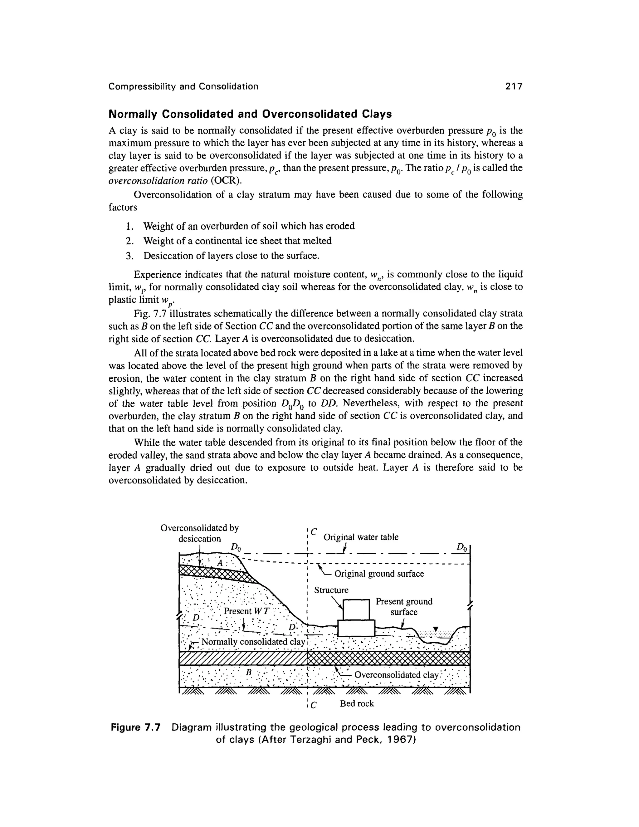
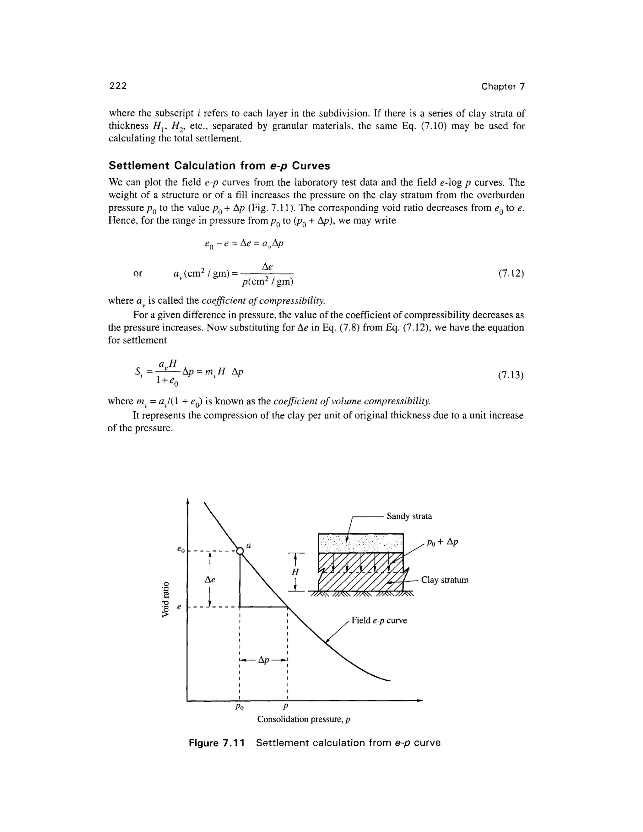
238. Compressibility an d Consolidation 21 9
7.7 e-log p FIEL D CURVE S FO R NORMALLY CONSOLIDATE D AN D
OVERCONSOLIDATED CLAYS O F LOW TO MEDIU M SENSITIVIT Y
It has been explaine d earlie r wit h reference t o Fig. 7.5, tha t the laborator y e-lo g p curv e of an
undisturbed sample does not pass through point A and always passes below the point. It has been
found fro m investigatio n tha t th e incline d straigh t portio n o f e-log p curve s o f undisturbe d or
remolded sample s of clay soil intersect a t one point at a low void ratio and corresponds t o 0.4eQ
shown as point C in Fig. 7.9 (Schmertmann, 1955). It is logical to assume the field curve labelled as
Kf shoul d als o pas s throug h thi s point . Th e fiel d curv e ca n b e draw n fro m poin t A, havin g
coordinates (e Q, /?0), which corresponds t o the in-situ condition of the soil. The straight line AC in
Fig. 7.9(a) gives the field curve AT,for normally consolidated clay soil of low sensitivity.
The field curve for overconsolidated cla y soil consists of two straight lines, represented by
AB and BC in Fig. 7.9(b). Schmertmann (1955) has shown that the initial section AB of the field
curve is parallel to the mean slope MNof th e rebound laboratory curve. Point B is the intersection
point of the vertical line passing through the preconsolidation pressure pc on the abscissa an d the
sloping line AB. Sinc e point C is the intersection of the laboratory compressio n curv e and the
horizontal line at void ratio 0.4eQ, line BC can be drawn. The slope of line MN whic h i s the slope
of the rebound curve is called the swell index Cs.
Clay o f Hig h Sensitivit y
If th e sensitivit y St i s greate r tha n abou t 8 [sensitivit y is define d a s th e rati o o f unconfme d
compressive strengths of undisturbed and remolded soi l samples refer to Eq. (3.50)], then the clay
is said to be highly sensitive. The natural water contents of such clay are more than the liquid
limits. Th e e-log p curv e K u fo r a n undisturbe d sampl e o f suc h a clay wil l hav e th e initia l
branch almost flat as shown in Fig. 7.9(c) , and after this it drops abruptly into a steep segment
indicating there b y a structural breakdown o f the clay suc h that a slight increase of pressur e
leads t o a large decrease in void ratio. The curve then passes through a point of inflection a t d
and its slope decreases . If a tangent is drawn at the point of inflection d, it intersects th e line
eQA a t b . The pressur e correspondin g t o b (p b) i s approximatel y equa l t o tha t a t whic h th e
structural breakdown take s place . I n areas underlain by soft highl y sensitive clays, the exces s
pressure Ap over the layer should be limited to a fraction of the difference of pressure (pt-p0).
Soil o f this type belongs mostl y to volcanic regions .
7.8 COMPUTATIO N O F CONSOLIDATION SETTLEMEN T
Settlement Equation s for Normall y Consolidate d Clays
For computin g th e ultimat e settlemen t o f a structur e founde d o n cla y th e followin g dat a ar e
required
1. Th e thickness of the clay stratum, H
2. Th e initial void ratio, eQ
3. Th e consolidation pressur e pQ or pc
4. Th e field consolidation curve K,
The slope of the field curve K.on a semilogarithmic diagram is designated a s the compression
index Cc (Fig. 7.9 )
The equation for Cc may be written as
C e
°~e e
°~e A g
Iogp-logp0 logp/ Po logp/p Q
(7
'4)

239. 220 Chapter 7
0.46>0
Remolded
compression curv e
Laboratory
compression
curve of an
undisturbed
sample ku
Field curve
K,
Po P
lOg/7
(a) Normally consolidated clay soil
A b
Laboratory compressio n curv e
Ae Field curve
or virgin
compression
curve
Po PC Po +
logp
(b) Preconsolidated cla y soil
0.4 e
PoPb
e-log p curve
(c) Typical e-log p curve for an undisturbed sample of clay of high sensitivity (Peck et al., 1974)
Figure 7. 9 Fiel d e-lo g p curve s
In one-dimensiona l compression , a s pe r Eq . (7.2) , th e chang e i n heigh t A/ / pe r uni t of
original H ma y b e writte n a s equa l t o th e chang e i n volum e AV per uni t o f origina l volum e V
(Fig. 7.10).
Art _ A V
H ~ V
Considering a unit sectiona l area of the clay stratum, we may write
(7.5)
Vl=Hl
= Hs (e Q -

240. Compressibility and Consolidation 221
H
f
n,
I J
A//
Figure 7.10 Chang e of height due to one-dimensiona l compressio n
Therefore,
Substituting for AWVin Eq. (7.5)
Ae
(7.6)
(7.7)
If we designate the compression A// of the clay layer as the total settlement St of the structure
built on it, we have
A// = S =
l + er
(7.8)
Settlement Calculatio n fro m e-lo g p Curve s
Substituting for Ae in Eq. (7.8) we have
Po
or •/flog-
Po
(7.9)
(7.10)
The net change in pressure Ap produced b y the structure a t the middle o f a clay stratu m is
calculated from the Boussinesq o r Westergaard theories as explained in Chapter 6.
If the thickness of the clay stratum is too large, th e stratum may be divided into layers of
smaller thickness not exceeding 3 m. The net change in pressure A/? at the middle of each layer will
have to be calculated. Consolidatio n tests wil l have to be completed o n samples take n from th e
middle of each of the strata and the corresponding compression indices will have to be determined.
The equation for the total consolidation settlement may be written as
(7.11)

241. 222 Chapter 7
where th e subscrip t; ' refers t o each laye r i n the subdivision . If there i s a series o f cla y strat a of
thickness H r // 2, etc. , separate d b y granula r materials , th e sam e Eq . (7.10 ) ma y b e use d fo r
calculating the total settlement.
Settlement Calculatio n fro m e- p Curve s
We can plo t th e fiel d e- p curve s from the laborator y test dat a an d th e fiel d e-og p curves . Th e
weight of a structure or of a fill increases th e pressure o n the clay stratum from th e overburden
pressure pQ t o the valu e p() + A/? (Fig. 7.11). The correspondin g voi d ratio decreases fro m eQ to e .
Hence, for th e range in pressure from pQ t o (pQ + A/?), we may writ e
-e -
or av (cm2
/gm) = (7.12)
/?(cm2
/gin)
where av is called th e coefficient o f compressibility.
For a given difference in pressure, the value of the coefficient of compressibility decreases as
the pressure increases . No w substituting for Ae in Eq. (7.8) from Eq . (7.12), we have the equation
for settlement
a H
S; = —-—Ap = mvH A/ ? (7.13)
where mv = av/( 1 + eQ) is known as the coefficient o f volume compressibility.
It represents th e compression o f the clay per unit of original thickness due to a unit increas e
of the pressure .
Clay stratum
Po P
Consolidation pressure, p
Figure 7.11 Settlemen t calculatio n fro m e-p curve

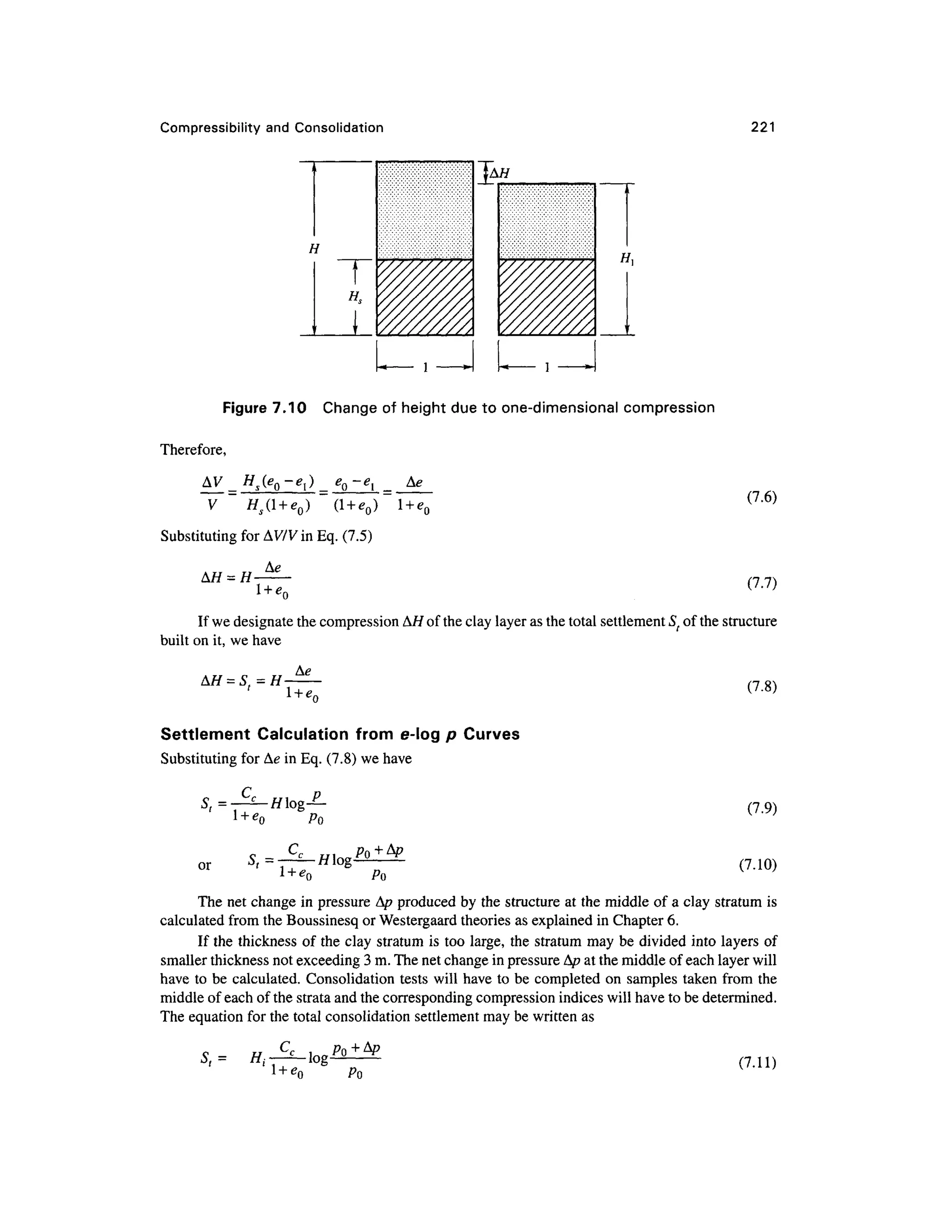
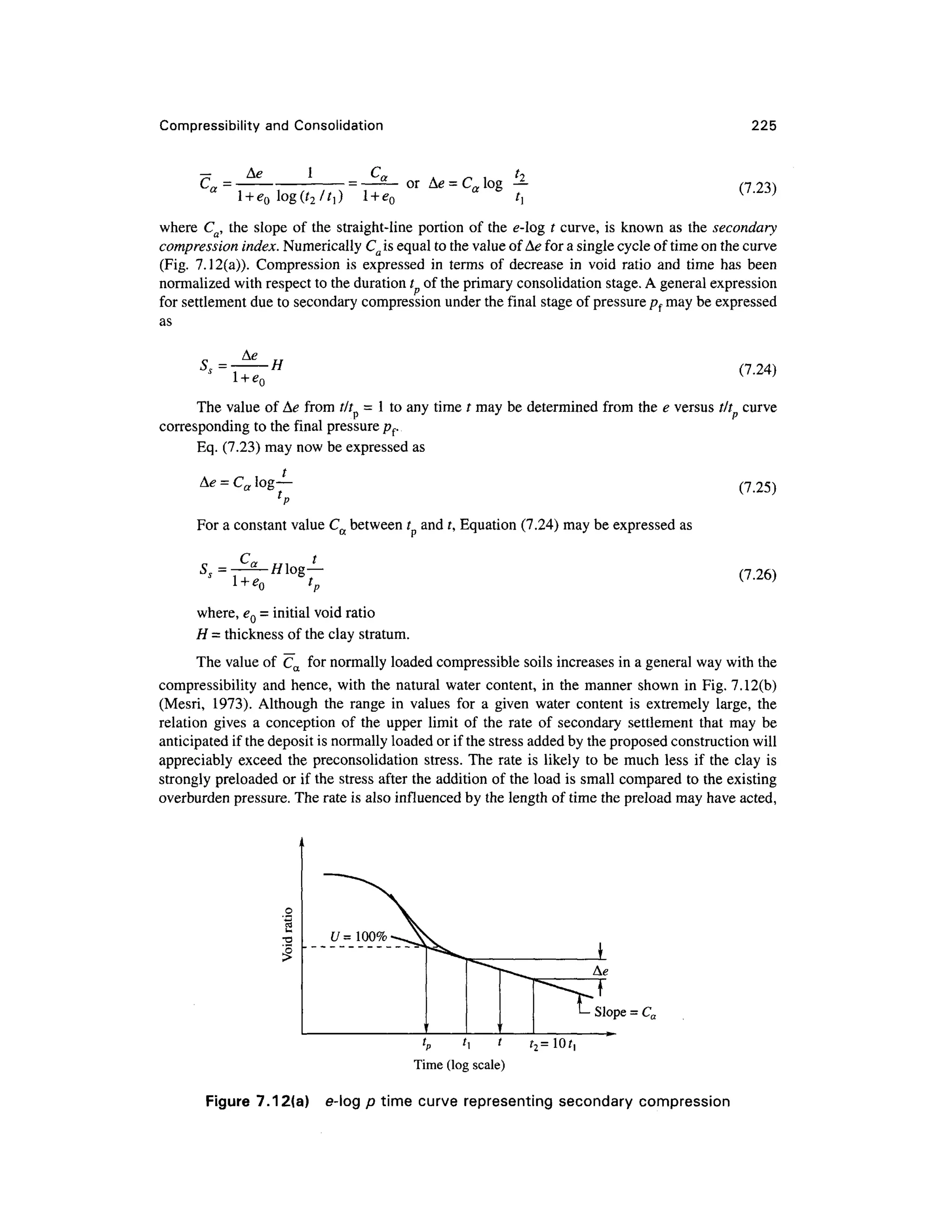
242. Compressibility and Consolidation 22 3
Settlement Calculatio n from e-log p Curv e fo r Overconsolidate d Cla y Soi l
Fig. 7.9(b) gives the field curve Kffor preconsolidate d clay soil. The settlement calculation depends
upon the excess foundation pressure Ap over and above the existing overburden pressure pQ.
Settlement Computation , i f pQ + A/0 < pc (Fig . 7.9(b))
In such a case, us e the sloping line AB. If Cs = slope of this line (also called the swell index), we
have
a
c =
log(p
o+Ap)
(7.14a )
Po
or A * = C, log
^ (7.14b )
By substituting for A< ? in Eq. (7.8) , we have
(7.15a)
Settlement Computation , if p0 < pc < p0 + Ap
We may write from Fig. 7.9(b)
Pc
(715b)
In this case the slope of both the lines AB and EC in Fig. 7.9(b) are required to be considered.
Now the equation for St may be written as [from Eq. (7.8) and Eq. (7.15b)]
CSH p c C CH
log— + — -—log
* Pc
The swell index Cs « 1/ 5 to 1/10 Cc can be used as a check.
Nagaraj an d Murthy (1985) have proposed the following equation for Cs as
C = 0.046 3 -^ - G
100 s
where wl = liquid limit, Gs = specific gravity of solids.
Compression Inde x C c — Empirica
l Relationship s
Research workers in different part s of the world have established empirica l relationships between
the compression index C and other soil parameters. A few of the important relationships are given
below.
Skempton's Formul a
Skempton (1944) established a relationship between C, and liquid limits for remolded clay s as
Cc = 0.007 (wl - 10 ) (7.16 )
where wl is in percent.

243. 224 Chapte r 7
Terzaghi and Pec k Formul a
Based o n th e wor k o f Skempto n an d others , Terzagh i an d Pec k (1948 ) modifie d Eq . (7.16 )
applicable to normally consolidated clays of low to moderate sensitivity as
Cc = 0.009 (w, -10) (7.17 )
Azzouz e t al. , Formul a
Azzouz e t al. , (1976 ) propose d a numbe r of correlation s base d o n th e statistica l analysi s o f a
number of soils. The one of the many which is reported t o have 86 percent reliability is
Cc = 0.37 (e Q + 0.003 w{ + 0.0004 wn - 0.34 ) (7.18 )
where eQ = in-situ void ratio, wf an d wn are in per cent. For organic soil they proposed
Cc = 0.115wn (7.19 )
Hough's Formul a
Hough (1957) , o n th e basi s o f experiment s o n precompresse d soils , ha s give n th e following
equation
Cc = 0.3 (e0- 0.27) (7.20 )
Nagaraj an d Srinivas a Murth y Formul a
Nagaraj an d Srinivas a Murthy (1985 ) hav e develope d equation s based o n thei r investigatio n a s
follows
Cc = 0.2343 e, (7.21 )
Cc = 0.39*0 (7.22 )
where el is the void ratio at the liquid limit, and eQ is the in-situ void ratio.
In the absence of consolidation test data, one of the formulae given above may be used for
computing Cc according to the judgment of the engineer.
7.9 SETTLEMEN T DU E TO SECONDAR Y COMPRESSIO N
In certain types of clays the secondary time effects ar e very pronounced to the extent that in some
cases th e entir e time-compressio n curv e has th e shap e o f a n almos t straigh t slopin g lin e when
plotted o n a semilogarithmi c scale , instea d o f th e typica l inverte d S-shap e wit h pronounce d
primary consolidation effects. These so called secondary time effects are a phenomenon somewha t
analogous t o th e cree p o f othe r overstresse d materia l i n a plasti c state . A delaye d progressiv e
slippage of grain upon grain as the particles adjust themselves to a more dense condition, appears to
be responsible for the secondary effects. When the rate of plastic deformations of the individual soil
particles o r of their slippage on each othe r is slower than the rate of decreasing volum e of voids
between the particles, then secondary effects predominat e and this is reflected b y the shape of the
time compression curve. The factors which affect the rate of the secondary compression of soils are
not ye t full y understood , and n o satisfactor y method has ye t bee n develope d fo r a rigorous an d
reliable analysis and forecast of the magnitude of these effects. Highl y organic soils are normally
subjected to considerable secondary consolidation.
The rat e o f secondar y consolidatio n ma y b e expresse d b y th e coefficient o f secondary
compression, C a a s

244. Compressibility and Consolidation 225
c = cn or A e = Ca log —
*
(7.23)
where Ca, the slop e of the straight-lin e portio n o f the e-log t curve, is known a s the secondary
compression index. Numerically Ca is equal to the value of Ae for a single cycle of time on the curve
(Fig. 7.12(a)) . Compressio n i s expresse d i n term s o f decreas e i n voi d rati o an d tim e has bee n
normalized with respect to the duration t o f the primary consolidation stage. A general expression
for settlement due to secondary compression under the final stage of pressure pf ma y be expressed
as
5 = •H (7.24)
The value of Ae from tit = 1 to any time / may be determined fro m th e e versus tit curv e
corresponding to the final pressure pf.
Eq. (7.23) may now be expressed as
A<? = Ca log —
For a constant value Ca between t an d t, Equation (7.24) may be expressed as
(7.25)
(7.26)
where, eQ - initia l void ratio
H = thickness of the clay stratum.
The value of C a fo r normally loaded compressible soil s increases i n a general way with the
compressibility an d hence, wit h the natural water content, in the manner show n in Fig. 7.12(b)
(Mesri, 1973) . Althoug h th e rang e i n value s fo r a give n wate r conten t i s extremel y large , th e
relation give s a conceptio n o f th e uppe r limi t of th e rat e o f secondar y settlemen t tha t may b e
anticipated if the deposit is normally loaded or if the stress added by the proposed construction will
appreciably excee d th e preconsolidation stress . Th e rate i s likely t o be muc h less if the clay is
strongly preloaded o r if the stress afte r th e addition of the load is small compared t o the existing
overburden pressure. The rate is also influenced by the length of time the preload ma y have acted,
Slope = Ca
r2 =10f,
Time (log scale)
Figure 7.12(a) e-lo g p time curve representin g secondar y compressio n

245. 226 Chapter 7
100
10
1.0-
0.1
10
1. Sensitiv e marine clay, Ne w
Zealand
2. Mexic o city clay
3. Calcareou s organic clay
4. Led a clay
5. Norwegia n plastic clay
6. Amorphou s and fibrous peat
7. Canadia n muskeg
8. Organi c marine deposits
9. Bosto n blue clay
10. Chicag o blue clay
11. Organi c silty clay
O Organi c silt, etc .
100
Natural water content, percent
1000 3000
Figure 7.12(b) Relationshi p betwee n coefficien t o f secondary consolidatio n an d
natural wate r conten t of normall y loade d deposits o f clays and various compressibl e
organic soil s (after Mesri, 1973 )
by the existence of shearing stresses and by the degree of disturbance of the samples. The effects of
these various factors have not yet been evaluated. Secondary compression i s high in plastic clays
and organic soils. Table 7.1 provides a classification of soil based on secondary compressibility . If
'young, normally loaded clay', having an effective overburden pressure of p0 is left undisturbed for
thousands of years, there will be creep or secondary consolidation. This will reduce the void ratio
and consequentl y increas e th e preconsolidatio n pressur e whic h wil l b e muc h greate r tha n th e
existing effectiv e overburde n pressur e p Q. Suc h a cla y ma y b e calle d a n aged, normally
consolidated clay.
Mesri and Godlewski (1977) report that for any soil the ratio Ca/Cc is a constant (where Cc is
the compression index) . This is illustrated in Fig. 7.13 for undisturbed specimens of brown Mexico
City clay with natural water content wn = 313 to 340%, vv ; = 361%, w p = 9% andpc/po = 1. 4
Table 7.2 gives values of Ca/Ccfor some geotechnical material s (Terzaghi, et al., 1996) .
It is reported (Terzaghi e t al., 1996 ) tha t for all geotechnical material s C a/Cc ranges fro m
0.01 to 0.07. Th e value 0.04 i s the most common value for inorganic clays and silts.

246. Compressibility an d Consolidation 227
0.3
0.2
•o
§
0.1
ii
Mexico City clay
calcc = 0.046
0 1 2 3 4 5 6
Compression index Cc
Figure 7.13 A n example of the relatio n betwee n C a and Cc (after Mesri and
Godlewski, 1977 )
Table 7.1 Classificatio n of soil based on secondary compressibility (Terzaghi ,
et al., 1996)
C Secondar y compressibilit y
< 0.002
0.004
0.008
0.016
0.032
0.064
Very low
Low
Medium
High
Very high
Extremely high
Table 7.2 Value s of C aICc for geotechnica l material s (Terzaghi, et al., 1996 )
Material
Granular soils including rockfill 0.0 2 ± 0.01
Shale and mudstone 0.0 3 ± 0.01
Inorganic clay and silts 0.0 4 ± 0.01
Organic clays and silts 0.0 5 ± 0.01
Peat and muskeg 0.0 6 ± 0.01
Example 7. 1
During a consolidation test, a sample of fully saturated clay 3 cm thick (= hQ) is consolidated under
a pressure increment of 200 kN/m2
. When equilibrium is reached, the sample thickness is reduced
to 2.60 cm. The pressure is then removed and the sample is allowed to expand and absorb water.
The final thickness is observed as 2.8 cm (ft,) and the final moisture content is determined as 24.9%.

247. 228 Chapter 7
K, = 0.672 cm3
Figure Ex. 7. 1
If the specific gravity of the soil solids is 2.70, find the void ratio of the sample befor e and afte r
consolidation.
Solution
Use equation (7.3 )
-
h
A/z
1. Determination of 'e*
Weight of solids = Ws = VsGs Jm = 1 x 2.70 x 1 =2.70 g.
W
W
= 0.249 or Ww = 0.249 x 2.70 = 0.672 gm, e f = Vw= 0.672.
2. Changes i n thickness from final stage to equilibrium stage with load on
(1 +0.672)0.20
A/i = 2.80 -2.60 = 0.20 cm ,
2.80
• = 0.119.
Void ratio afte r consolidation = e,-&e = 0.672 - 0. 1 19 = 0.553.
3. Change i n void ratio fromth e commencement t o the end of consolidation
1 +0
-553
(3.00 - 2.60) = x 0.40 = 0.239 .
2.6 2. 6
Void ratio at the start of consolidation = 0.553 + 0.239 = 0.792
Example 7. 2
A recently completed fil l wa s 32.8 ft thick and its initial average voi d ratio was 1.0 . The fill was
loaded o n th e surfac e b y constructin g an embankmen t coverin g a larg e are a o f th e fill . Som e
months after the embankment was constructed, measurements of the fill indicated an average void
ratio of 0.8. Estimate the compression of the fill .

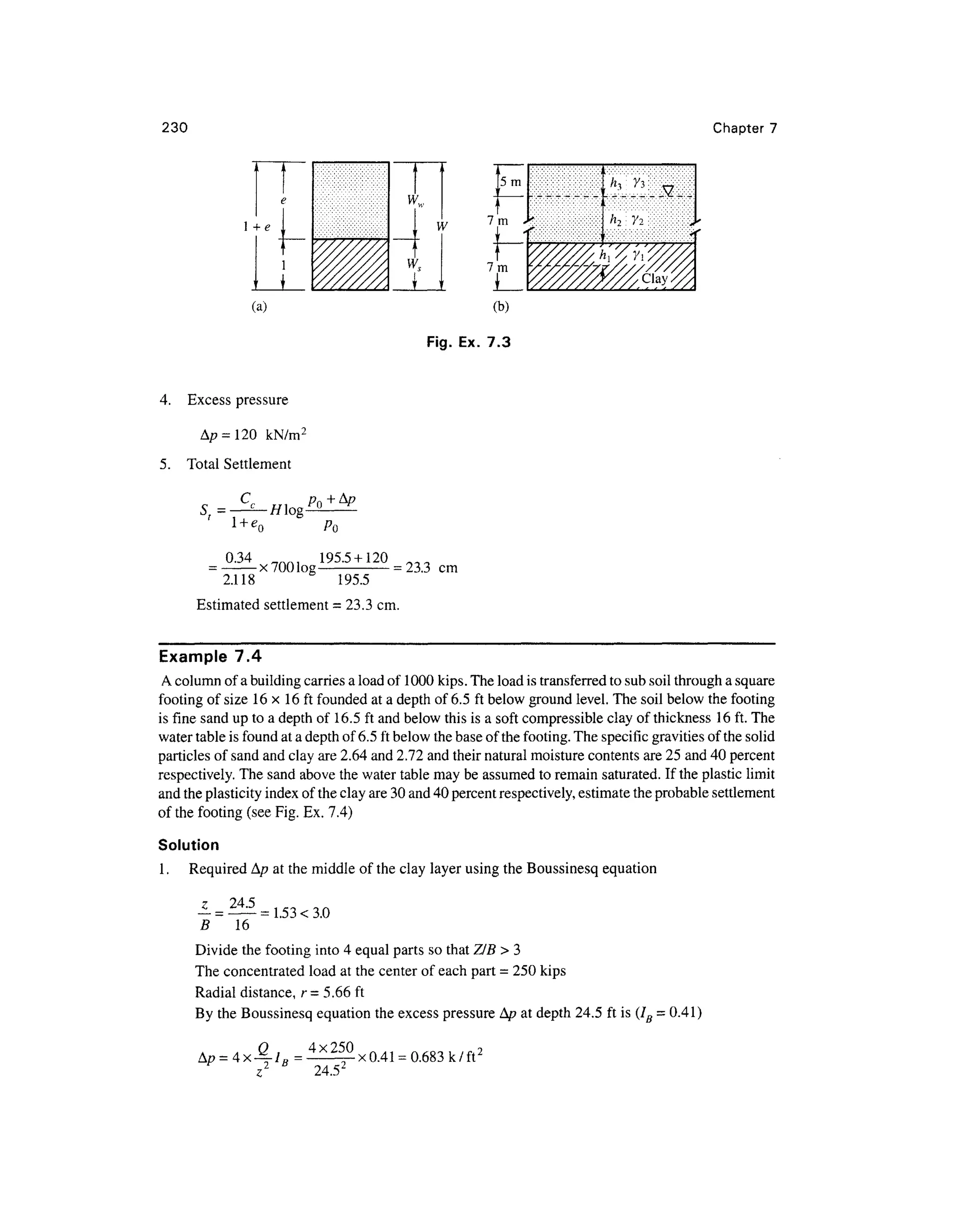
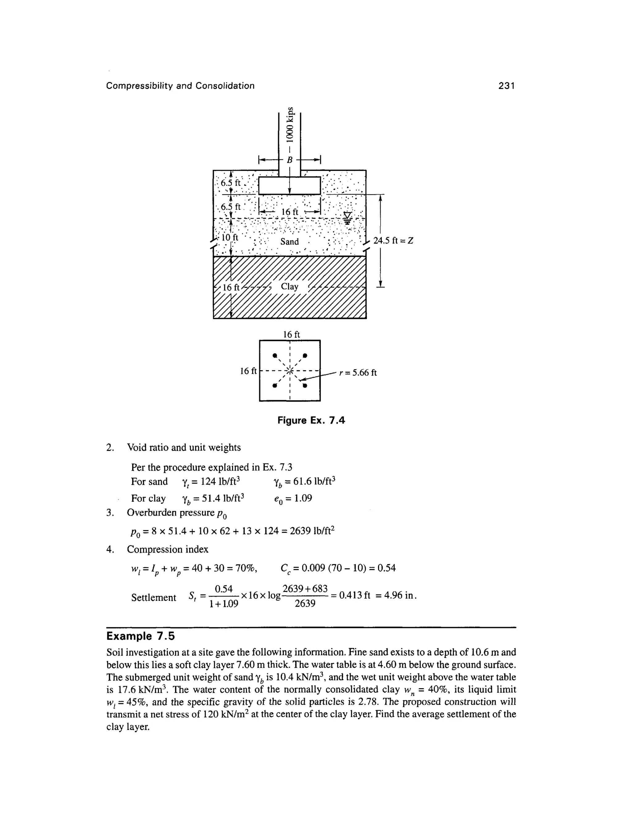
248. Compressibility and Consolidation 22 9
Solution
Per Eq. (7.7), the compression of the fill may be calculated as
where AH = the compression, Ae = change in void ratio, eQ = initial void ratio, HQ = thickness of fill.
Substituting, A/ f = L0
~0
-8
x 32.8 = 3.28 ft .
Example 7. 3
A stratum of normally consolidated clay 7 m thick is located a t a depth 12 m below ground level.
The natura l moisture content of the clay is 40.5 pe r cent and its liquid limit is 48 per cent. The
specific gravity of the solid particles is 2.76. The water table is located at a depth 5 m below ground
surface. The soil is sand above the clay stratum. The submerged unit weight of the sand is 1 1 kN/m3
and the same weighs 1 8 kN/m3
above the water table. The average increase in pressure at the center
of the clay stratum is 120 kN/m2
due to the weight of a building that will be constructed on the sand
above the clay stratum. Estimate the expected settlemen t of the structure.
Solution
1 .Determinatio n of e and yb for the clay [Fig. Ex. 7.3]
W
=1x2.76x1 =2.76 g
405
W = — x2.7 6 =1.118 g
w
10 0
„
r
vs i
= UI& + 2.76 = 3.878 g
W
' 1 Q - J / 3
Y, = -
= -
=1-83 g/c m
' 2.11 8
Yb = (1.83-1 ) = 0.83 g/cm 3
.
2. Determinatio n of overburden pressure p Q
PO = yh
i+ Y2h
i+ yA°r
P0= 0.83x9.81x3.5 + 11x7 + 18x5 = 195.5 kN/m 2
3. Compressio n inde x [Eq. 11.17 ]
Cc = 0.009(w, -10) = 0.009 x(48 -10
) =0.34

249. 230 Chapter 7
w
w.
5m
7m J
7m
I
(b)
Fig. Ex . 7. 3
4. Exces s pressure
A;? = 120 kN/m 2
5. Tota l Settlement
C
st =
0.34 __ n i 195. 5 + 120 00 0
x 700 log
= 23.3 c m
2.118 " 195. 5
Estimated settlement = 23.3 cm.
Example 7. 4
A column of a building carries a load of 1000 kips. The load is transferred to sub soil through a square
footing of size 16 x 1 6 ft founded at a depth of 6.5 ft below ground level. The soil below the footing
is fine sand up to a depth of 16.5 ft and below this is a soft compressible cla y of thickness 1 6 ft. The
water table is found at a depth of 6.5 ft below the base of the footing. The specific gravities of the solid
particles of sand and clay are 2.64 and 2.72 and their natural moisture contents are 25 and 40 percent
respectively. The sand above the water table may be assumed to remain saturated. If the plastic limit
and the plasticity index of the clay are 30 and 40 percent respectively, estimate the probable settlement
of the footing (see Fig. Ex. 7.4)
Solution
1. Require d A/? at the middle of the clay layer using the Boussinesq equation
24.5
16
= 1.53 <3.0
Divide the footing into 4 equal parts so that Z/B > 3
The concentrated loa d at the center of each part = 250 kips
Radial distance, r = 5.66 ft
By the Boussinesq equation the excess pressure A/? at depth 24.5 ft is (IB = 0.41 )
0.41 = 0.683k/ft2
24.5'

250. Compressibility and Consolidatio n 231
. - . * ' . .•
.•6.5 ft W.
CX
3
^^ferief,.
24.5 ft = Z
16ft
16ft - r = 5.66 ft
Figure Ex. 7. 4
2. Voi d ratio and unit weights
Per the procedure explained in Ex. 7.3
For san d y , = 12 4 lb/ft3
y fc = 61.6 lb/ft3
For clay y b = 51.4 lb/ft3
<? 0 = 1.09
3. Overburde n pressure p Q
pQ = 8 x 51.4 + 10 x 62 + 13 x 12 4 = 2639 lb/ft 2
4. Compressio n inde x
w/ = Ip + wp = 40 + 30 =70%, C c = 0.009 (70 - 10 ) =0.54
0.54 ... . 263 9 +68
3 ft/lia A A 0, .
Settlement S , = . ._x!6xlo g
= 0.413 ft = 4.96m.
1 +1.09 2639
Example 7. 5
Soil investigation at a site gave the following information. Fine sand exists to a depth of 10.6 m and
below this lies a soft clay layer 7.60 m thick. The water table is at 4.60 m below the ground surface.
The submerged unit weight of sand yb is 10.4 kN/m3
, and the wet unit weight above the water table
is 17. 6 kN/m3
. Th e wate r conten t o f the normall y consolidated cla y w n = 40%, it s liqui d limit
wt = 45%, an d th e specific gravit y of the solid particle s i s 2.78. Th e proposed constructio n will
transmit a net stress of 120 kN/m2
at the center of the clay layer. Find the average settlement of the
clay layer.

251. 232 Chapte r 7
Solution
For calculating settlement [Eq. (7.15a)]
C p n + A/?
S = — —H log^ -
-wher e &p = 120 kN /m2
l + eQ p Q
From Eq. (7.17), Cr = 0.009 (w, - 10 ) =
0.009(45 - 10 ) =
0.32
wG
From Eq. (3. 14a), e Q = -
= wG = 0.40 x 2.78 =1.1 1sinc e S =1
tJ
Yb, the submerged unit weight of clay, is found as follows
MG.+«.) = 9*1(2.78 + Ul) 3
' ^" t 1 , 1 . 1 1 1
l + eQ l + l.ll
Yb=Y^-Yw = 18.1-9.8 1 =8.28 kN/m3
The effective vertical stress pQ a t the mid height of the clay layer is
pQ = 4.60 x 17.6 + 6 x10.4 + —x 8.28 = 174.8 kN / m2
_ 0.32x7.60 , 174. 8 + 120
Now S t = -
log -
=0.26m =26 cm
1
1+1.1 1 174. 8
Average settlement
= 2 6 cm.
Example 7. 6
A soil sampl e ha s a compression inde x of 0.3. I f the void ratio e at a stress o f 2940 Ib/ft2
i s 0.5,
compute (i ) the void ratio if the stress i s increased to 4200 Ib/ft2
, an d (ii) the settlement o f a soil
stratum 1 3 ft thick.
Solution
Given: C c = 0.3, el = 0.50, /?, = 2940 Ib/ft2
, p2 = 4200 Ib/ft2
.
(i) No w from Eq. (7.4),
p — p
C i
%."-)
C = l
- 2
—
or e 2 = e
]-c
substituting the known values, we have,
e- = 0.5 -0.31og - 0.454
2
294 0
(ii) Th e settlement per Eq. (7.10) is
c c
c „ , Pi 0.3x13x12 , 420 0
S = — —//log— = -
log -
=4.83 m
.
pl 1. 5 294 0

252. Compressibility an d Consolidation 23 3
Example 7. 7
Two points on a curve for a normally consolidated clay have the following coordinates.
Point 1 :*, = 0.7, Pl = 2089 lb/ft 2
Point 2: e2 = 0.6, p 2 = 6266 lb/ft 2
If th e averag e overburde n pressur e o n a 2 0 f t thic k cla y laye r i s 313 3 lb/ft2
, ho w muc h
settlement will the clay layer experience due to an induced stress of 3340 lb/ft2
at its middepth.
Solution
From Eq. (7.4) we have
C - e
^e
> = °- 7
"a6
-02 1
c
ogp 2/pl lo g (6266/2089)
We need the initial void ratio eQ at an overburden pressure of 3133 lb/ft 2
.
en -e~
C = —2 —T2
— = 0.21
or (eQ - 0.6 ) = 0.21 log (6266/3 133) = 0.063
or e Q = 0.6 + 0.063 = 0.663.
Settlement, s =
Po
Substituting the known values, with Ap = 3340 lb/ft2
„ 0.21x20x12 , 313 3 +3340 nee .
$ = -
log -
=9.55 in
1.663&
313 3
7.10 RAT E O F ONE-DIMENSIONAL CONSOLIDATIO N THEORY O F
TERZAGHI
One dimensional consolidation theory as proposed by Terzaghi is generally applicable in all cases
that arise in practice where
1. Secondar y compression is not very significant,
2. Th e clay stratum is drained on one or both the surfaces,
3. Th e clay stratum is deeply buried, and
4. Th e clay stratum is thin compared with the size of the loaded areas .
The following assumptions are made in the development of the theory:
1. Th e voids of the soil are completely filled with water,
2. Bot h water and solid constituents are incompressible,
3. Darcy' s la w is strictly valid,
4. Th e coefficient of permeability is a constant,
5. Th e time lag of consolidation is due entirely to the low permeability of the soil, and
6. Th e clay is laterally confined.

253. 234 Chapter 7
Differential Equatio n fo r One-Dimensiona l Flo w
Consider a stratu m o f soi l infinit e in exten t i n th e horizonta l directio n (Fig . 7.14) bu t o f suc h
thickness // , tha t th e pressure s create d b y th e weigh t o f th e soi l itsel f ma y b e neglecte d i n
comparison t o the applied pressure.
Assume that drainage takes place only at the top and further assume that the stratum has been
subjected to a uniform pressure of pQ fo r such a long time that it is completely consolidate d under
that pressur e an d tha t ther e i s a hydrauli c equilibriu m prevailing, i.e., th e wate r leve l i n th e
piezometric tub e a t an y sectio n X Y i n th e cla y stratu m stand s a t th e leve l o f th e wate r tabl e
(piezometer tube in Fig. 7.14).
Let a n incremen t of pressur e A/ ? b e applied . Th e tota l pressur e t o whic h th e stratu m is
subjected is
Pl=pQ + Ap(7.27 )
Immediately afte r the increment of load is applied the water in the pore space throughout the
entire height , H , wil l carr y th e additiona l loa d an d ther e wil l be se t u p a n exces s hydrostati c
pressure ui throughout the pore water equal to Ap as indicated in Fig. 7.14.
After an elapsed time t = tv some of the pore water will have escaped at the top surface and as a
consequence, the excess hydrostatic pressure will have been decreased and a part of the load transferred to
the soil structure. The distribution of the pressure between the soil and the pore water, pand u respectively
at any time t, may be represented by the curve as shown in the figure. It is evident that
Pi=p + u (7.28 )
at any elapsed time t and at any depth z, and u is equal to zero at the top. The pore pressure u, at any
depth, is therefore a function o f z and / and may be written as
u =f(z, t) (7.29)
Piezometers
Impermeable
(a) (b )
Figure 7.1 4 One-dimensiona l consolidatio n

254. Compressibility and Consolidation 23 5
Consider a n element o f volume of the stratum at a depth z, and thickness dz (Fig. 7.14). Let
the bottom and top surfaces o f this element have unit area.
The consolidation phenomenon is essentially a problem of non-steady flow of water through a
porous mass. The difference between the quantity of water that enters the lower surface at level X'Y'
and the quantity of water which escapes the upper surface at level XY in time element dt must equal the
volume change of the material which has taken place in this element of time. The quantity of water is
dependent on the hydraulic gradient which is proportional to the slope of the curve t .
The hydraulic gradients at levels XY and X'Y' of the element are
, 1 d du 1 du ^ 1 d 2
u ,
iss
^-*u+
**=
TwTz+
Tw^dz (7
-30)
If k is the hydraulic conductivity the outflow from the element at level XY in time dt is
k du
dql=ikdt = ——dt(7.31 )
' W **
The inflow at level X'Y' is
k du d 2
u
dq2 = ikdt= ~^dt+ -^dzdt(7.32 )
The difference in flow is therefore
k
dq = dq^ -dq 2 = -— -r-^dzd t (7.33 )
• w
From th e consolidatio n tes t performe d i n th e laboratory , i t i s possibl e t o obtai n th e
relationship between the void ratios corresponding to various pressures to which a soil is subjected.
This relationshi p i s expresse d i n th e for m o f a pressure-voi d rati o curv e whic h give s th e
relationship as expressed in Eq. (7.12)
de = avdp (7.34 )
The chang e i n volum e Ad v o f th e elemen t give n i n Fig . 7.14 may b e writte n a s pe r
Eq. (7.7).
de
Mv = Mz = - -
dz (7.35 )
i + e
Substituting for de, we have
(7.36)
Here dp is the change in effective pressure at depth z during the time element dt. The increas e
in effective pressure dp is equal to the decrease in the pore pressure, du.
du
Therefore, d p = -du = -^~dt(7.37 )
at

255. 236 Chapte r 7
av du du
Hence, Mv = —— dtdz = -tnv—dtdz (7.38 )
l + eat v
dt v
'
Since the soil is completely saturated , the volume change AJv of the element of thickness
dz i n time dt is equal to the change in volume of water dq in the same element i n time dt .
Therefore, d q = Mv (7.39 )
or
or
k d 2
u
-,- , di L
rw di 2
k( + e}d2
u
Ywav dz 2
a du
-it-i -if
u — , ^ az at
l + edt
dtv
dz 2
k
y a y m
' W V ' W V
is defined as the coefficient o f consolidation.
(7.40)
(7.41)
Eq. (7.40) is the differential equatio n for one-dimensional flow . The differential equation for
three-dimensional flow may be developed in the same way. The equation may be written as
du l + ed 2
u d 2
u d 2
u
(7
'42)
where kx, ky an d k z ar e the coefficients of permeability (hydraulic conductivity) in the coordinat e
directions of jc, y an d z respectively.
As consolidatio n proceeds , th e value s o f k , e an d av al l decreas e wit h tim e bu t th e rati o
expressed b y Eq. (7.41) may remain approximately constant.
Mathematical Solutio n fo r th e One-Dimensiona l Consolidatio n Equatio n
To solve the consolidation Eq. (7.40) it is necessary t o set up the proper boundary conditions. For
this purpose, conside r a layer of soil having a total thickness 2H and having drainage facilitie s at
both the top and bottom faces as shown in Fig. 7.15. Under this condition n o flow wil l take plac e
across th e cente r lin e a t depth H. The cente r lin e can therefor e b e considered a s a n impervious
barrier. The boundary conditions for solving Eq. (7.40) may be written as
1 .u = 0 when z = 0
2. u = 0 when z = 2H
3. u = <p for all depths at time t = 0
On th e basi s o f th e abov e conditions , th e solutio n o f th e differentia l Eq. (7.40 ) ca n b e
accomplished b y means of Fourier Series .
The solution is
mz _ m2r
u= - sin — eml
(7.43 )
m H
1)* c vt .
where m - -
,/ = — — = a non-dimensional time factor.
2 H 2
Eq. (7.43) can be expressed in a general form as

256. Compressibility an d Consolidation 237
H
H
Clay
'• San d y..'•:.':I
P
Figure 7.15 Boundar y condition s
~Kp=f
~H'T (7
'44)
Equation (7.44 ) ca n b e solve d b y assumin g T constant fo r variou s value s o f z/H. Curve s
corresponding to different value s of the time factorT may be obtained as given in Fig. 7.16. It is of
interest to determine how far the consolidation process under the increment of load Ap has progressed
at a time t corresponding t o the time factorT at a given depth z. The term £/ , is used to express this
relationship. It is defined as the ratio of the amount of consolidation which has already taken place to
the total amount which is to take place under the load increment.
The curves in Fig. 7.16 shows the distribution of the pressure Ap between solid and liquid phases
at various depths. At a particular depth, say z/H = 0.5, the stress in the soil skeleton is represented by AC
and the stress in water by CB. AB represents the original excess hydrostatic pressure ui =Ap. The degree
of consolidation U z percent at this particular depth is then
AC Ap- « u
u % = ioox—- = -t
-— = 100 i-—
z
A B A p A p (7.45)
r
1.0
A/7- U
0.5
z/H 1. 0
r=o
1.5
2.0
T= o o
Figure 7.16 Consolidatio n of cla y laye r as a function T

257. 238 Chapter 7
Following a similar reasoning, the average degree of consolidation U% for the entire layer at
a time factor Tis equal to the ratio of the shaded portion (Fig. 7.16) of the diagram to the entire area
which is equal to 2H A/? .
Therefore
2H
U% =u
_. . xlO O
2H
or £/ % = 2H —— udz
2H ^p
o
Hence, Eq. (7.46) afte r integration reduces t o
(7.46)
£/%=100 1 - — -£ -m2
T
(7.47)
It can be seen from Eq. (7.47) that the degree of consolidation is a function of the time factor T
only which is a dimensionless ratio. The relationship between Tand U% may therefore be established
once an d fo r al l b y solvin g Eq. (7.47 ) fo r variou s value s of T . Values thus obtained ar e give n in
Table 7.3 and also plotted on a semilog plot as shown in Fig. 7.17.
For value s o f U% betwee n 0 an d 60% , th e curv e i n Fig . 7.17 ca n b e represente d almos t
exactly by the equation
T =
4 10 0
which is the equation of a parabola. Substitutin g for T, Eq. (7.48) may be written as
U%
oo
(7.48)
(7.49)
u%
u
20
40
60
80
100
O.C
—• —„
--
,
k
^^
)03 0.0 1 0.0 3 0. 1 0. 3 1. 0 3. 0 1 0
Time factor T(log scale)
Figure 7.1 7 U versus T

258. Compressibility and Consolidation 239
Table 7.3 Relationshi p betwee n U and T
u%
0
10
15
20
25
30
35
T
0
0.008
0.018
0.031
0.049
0.071
0.096
U%
40
45
50
55
60
65
70
T
0.126
0.159
0.197
0.238
0.287
0.342
0.405
U%
75
80
85
90
95
100
T
0.477
0.565
0.684
0.848
1.127
oo
In Eq. (7.49), th e values of cv and H are constants. On e can determine th e time required t o
attain a given degree of consolidation b y using this equation. It should be noted that H represent s
half th e thicknes s o f th e cla y stratu m when the layer is drained o n both sides , an d i t is th e ful l
thickness whe n drained on one side only.
TABLE 7.4 Relatio n betwee n U % an d T (Specia l Cases)
Permeable Permeable
U%
Impermeable
Case 1
Impermeable
Case 2
Time Factors, T
Consolidation pressure
increase with depth
Consolidation pressure
decreases with depth
00
10
20
30
40
50
60
70
80
90
95
100
0
0.047
0.100
0.158
0.221
0.294
0.383
0.500
0.665
0.94
1
oo
0
0.003
0.009
0.024
0.048
0.092
0.160
0.271
0.44
0.72
0.8
oo

259. 240 Chapte r 7
For values of U% greater than 60%, the curve in Fig. 7.17 may be represented by the equation
T= 1.781 - 0.933 log (100 - U% ) (7.50 )
Effect o f Boundar y Condition s o n Consolidatio n
A layer of clay which permits drainage through both surfaces is called an open layer. The thickness
of such a layer is always represented b y the symbol 2H, in contrast to the symbol H use d for th e
thickness of half-closed layers which can discharge their excess wate r only through one surface.
The relationship expressed betwee n rand (/given in Table 7.3 applies to the following cases:
1. Wher e th e cla y stratu m is draine d o n bot h side s an d th e initia l consolidatio n pressur e
distribution is uniform o r linearly increasing or decreasing with depth.
2. Wher e the clay stratum i s drained on one sid e but the consolidation pressure i s uniform
with depth.
Separate relationship s between T and U are required for half closed layer s wit h thickness H
where the consolidation pressures increase or decrease with depth. Such cases are exceptional and
as such not dealt with in detail here. However, the relations between U% and7 " for these two cases
are given in Table 7.4 .
7.11 DETERMINATIO N O F THE COEFFICIENT O F CONSOLIDATION
The coefficien t of consolidatio n c ca n b e evaluate d by mean s o f laborator y test s b y fittin g th e
experimental curve with the theoretical.
There are two laboratory methods that are in common use for the determination of cv. They
are
1. Casagrand e Logarith m o f Time Fitting Method.
2. Taylo r Square Root of Time Fitting Method.
Logarithm o f Tim e Fittin g Metho d
This method wa s proposed b y Casagrande an d Fadum (1940).
Figure 7.18 i s a plo t showin g th e relationshi p between compressio n dia l readin g an d th e
logarithm of time of a consolidation test. The theoretical consolidation curve using the log scale for
the tim e facto r i s als o shown . Ther e i s a similarit y o f shap e betwee n th e tw o curves . O n th e
laboratory curve , th e intersectio n formed b y th e fina l straigh t lin e produce d backwar d an d th e
tangent to the curve at the point of inflection is accepted a s the 100 per cent primary consolidation
point an d th e dia l readin g i s designated a s /?100. The time-compressio n relationshi p in the early
stages is also parabolic just as the theoretical curve. The dial reading at zero primary consolidation
RQ can be obtained by selecting any two points on the parabolic portion of the curve where times are
in the ratio of 1 : 4. The differenc e i n dial readings between thes e tw o points is then equal to the
difference between the first point and the dial reading corresponding t o zero primary consolidation.
For example, two points A and B whose times 10 and 2.5 minutes respectively, are marked on the
curve. Let z{ b e the ordinate difference between the two points. Apoint C is marked vertically over
B such that BC = zr Then the point C corresponds to zero primary consolidation. The procedure is
repeated wit h several points. An average horizontal line is drawn through these points to represent
the theoretical zero percent consolidation line.
The interva l betwee n 0 an d 100 % consolidatio n i s divided int o equal interval s of percen t
consolidation. Since it has been foun d tha t th e laborator y an d th e theoretical curve s hav e better

260. Compressibility an d Consolidation 241
Asymptote
Rf-
f i/4
t } lo g (time )
(a) Experimental curve (b ) Theoretical curve
Figure 7.18 Lo g of time fitting method
correspondence a t the central portion , th e value of cy is computed by taking the time t and time
factor T at 50 percent consolidation. The equation to be used is
T
-~H
lr (7.51 )
T -
1
5Q
c t
v 5 0
or
l
dr
where Hdr = drainage path
From Table 7.3, we have at U = 50%, T= 0.197. From the initial height //. of specimen and
compression dial reading at 50% consolidation, Hdr fo r double drainage is
H: ~
(7.52)
where hH= Compression o f sample up to 50% consolidation.
Now the equation for c ma y be written as
c = 0.197
H
(7.53)
Square Roo t o f Tim e Fittin g Metho d
This method was devised by Taylor (1948). In this method, the dial readings are plotted against the
square root of time as given in Fig. 7.19(a). The theoretical curve U versus ^JT i s also plotted and
shown in Fig. 7.19(b). On the theoretical curve a straight line exists up to 60 percent consolidation
while at 90 percent consolidation the abscissa of the curve is 1.15 times the abscissa of the straight
line produced.
The fitting method consists of first drawing the straight line which best fits the early portion of the
laboratory curve. Next a straight line is drawn which at all points has abscissa 1.15 times as great as those
of the first line. The intersection of this line and the laboratory curve is taken as the 90 percent (R QQ)
consolidation point. Its value may be read and is designated as tgQ.

261. 242 Chapter 7
(a) Experimental curve (b ) Theoretical curve
Figure 7.19 Squar e root of time fitting method
Usually the straight line through the early portion of the laboratory curve intersects the zero
time line at a point (R o) differin g somewha t fro m the initial point (/? f.). This intersectio n poin t is
called th e corrected zero point. If one-ninth of th e vertica l distance betwee n th e correcte d zer o
point and the 90 per cent point is set off below the 90 percent point, the point obtained is called the
"100 percent primary compression point" (R loo). Th e compression between zero and 100 per cent
point is called "primary compression".
At the point of 90 percent consolidation, the value of T = 0.848. The equation of cv may now
be written as
H2
c = 0.848- ^ (7.54)
'90
where H, - drainag e path (average)
7.12 RAT E OF SETTLEMENT DU E TO CONSOLIDATIO N
It has been explaine d tha t the ultimate settlement St of a clay layer due t o consolidation may b e
computed b y usin g either Eq . (7.10 ) o r Eq . (7.13) . I f S i s the settlemen t a t an y tim e t after th e
imposition o f loa d o n th e cla y layer, the degre e o f consolidatio n o f th e laye r i n tim e t may b e
expressed a s
U% = — x 100 percent
Since U is a function o f the time factor T, we may write
(7.55)
= —xlOO
O
(7.56)
The rat e o f settlemen t curve of a structur e built on a cla y laye r ma y b e obtaine d b y th e
following procedure :

262. Compressibility an d Consolidation 243
Time t
Figure 7.20 Time-settlemen t curv e
1. Fro m consolidation test data, compute mv and cv.
2. Comput e the total settlement St that the clay stratum would experience wit h the increment
of load Ap.
3. Fro m the theoretical curve giving the relation between U and T, find T for different degrees
of consolidation, sa y 5, 10, 20, 30 percent etc.
TH2
,
4. Comput e from equation t = —— th e values of t for different value s of T. It may be noted
C
v
here that for drainage on both sides Hdr i s equal to half the thickness of the clay layer.
5. No w a curve can be plotted giving the relation between t and U% o r t and S as shown in
Fig. 7.20.
7.13 TWO - AND THREE-DIMENSIONAL CONSOLIDATION
PROBLEMS
When th e thicknes s o f a clay stratu m is great compare d wit h the widt h of the loaded area , th e
consolidation of the stratum is three-dimensional. In a three-dimensional proces s of consolidation
the flow occurs either in radial planes or else the water particles travel along flow lines which do not
lie in planes. The problem of this type is complicated though a general theory of three-dimensional
consolidation exists (Biot, et al., 1941). A simple example of three-dimensional consolidation is the
consolidation o f a stratu m o f sof t cla y o r sil t b y providin g san d drain s an d surcharg e fo r
accelerating consolidation .
The most important example of two dimensional consolidation in engineering practice is the
consolidation of the case of a hydraulic fill dam. In two-dimensional flow, the excess water drains
out of the clay in parallel planes. Gilboy (1934) has analyzed the two dimensional consolidation of
a hydraulic fill dam.
Example 7. 8
A 2.5 cm thick sample of clay was taken from th e field for predicting the time of settlement for a
proposed building which exerts a uniform pressure of 100 kN/m2
over the clay stratum. The sample
was loaded to 100 kN/m2
and proper drainage was allowed from top and bottom. It was seen that 50
percent of the total settlement occurred in 3 minutes. Find the time required for 50 percent of the

263. 244 Chapte r 7
total settlement of the building, if it is to be constructed on a 6 m thick layer of clay which extends
from th e ground surface and is underlain by sand.
Solution
Tfor 50% consolidation = 0.197.
The lab sample is drained on both sides. The coefficient of consolidation c i s found from
TH2
( 2 5)2
1
c = — =0.197 x —— x - = 10.25 x 10~2
cm2
/ min.
t 4 3
The tim e t for 50% consolidation in the field wil l be found as follows.
0.197x300x300x100 ,„„_ ,
t = :
= 120 days.
10.25x60x24
Example 7. 9
The void ratio of a clay sample A decreased from 0.572 to 0.505 under a change i n pressure fro m
122 to 180 kN/m2
. The void ratio of another sample B decreased from 0.61 to 0.557 under the same
increment of pressure. The thicknes s of sample A wa s 1. 5 times tha t of B. Nevertheless th e time
taken fo r 50 % consolidatio n wa s 3 time s large r fo r sampl e B tha n fo r A . Wha t i s th e rati o o f
coefficient o f permeability of sample A to that of Bl
Solution
Let H a = thicknes s o f sampl e A , H b = thicknes s o f sampl e B, m va = coefficien t o f volum e
compressibility o f sampl e A , m vb = coefficient o f volum e compressibilit y o f sampl e B , c va =
coefficient o f consolidation fo r sampl e A, cvb = coefficient of consolidation fo r sampl e B, A/?a =
increment o f loa d fo r sampl e A , A/? fe = incremen t o f loa d fo r sampl e B, k a = coefficien t o f
permeability for sample A, and kb = coefficient of permeability of sample B .
We may write the following relationship
Ae 1 A<? , l
m = -
a
- --—,m
h= -
b
- --—
va
+ eA w vb
l + e,Ap ,
a * a b rb
where e i s the void ratio of sample A at the commencement of the test and Aea is the change in void
ratio. Similarly eb and keb apply to sample B.
-, an d T = ^ K T , = ^fy-
wherein Ta, ta, Tb and tb correspond t o samples A and B respectively. We may write
c T H 2
t,
—=
"F^p* «= c
vam
varw>k
b = c
vbm
vbyw
vb b b a
k c m
™ r . a v a v a
Therefore, k c m
b vb vb
Given ea = 0.572, an d eb = 0.61
A<?= 0.572-0.50 5 = 0.067, Ae. =0.610-0.557 = 0.053
a ' o

264. Compressibility an d Consolidatio n 24 5
A D = Ap , = 180-122 = 58kN/m2
, H
= l.5H,
But t b
= 3t a
Q.Q67 1 + 0.61
a
We have, m = 0.053 * 1+ 0.572 = L29
vb
k
Therefore, T 2
-
= 6.75 x1.29 =8.7
K
b
The ratio is 8.7 : 1.
Example 7.1 0
A strat a o f normall y consolidate d cla y o f thicknes s 1 0 ft i s draine d o n on e sid e only . It ha s a
hydraulic conductivit y of h = 1.86 3 x 10~ 8
in/sec an d a coefficien t o f volum e compressibilit y
rav = 8.6 x 10"4
in2
/lb. Determine the ultimate value of the compression of the stratum by assuming
a uniformly distributed load of 5250 lb/ft2
and also determine the time required for 20 percent and
80 percent consolidation .
Solution
Total compression ,
S = m//A/ ? = 8.6 x10~4
x 10 x 12 x5250 x —= 3.763 in.
< v f 14 4
For determining the relationship between U% and T for 20% consolidation use the equation
n U% 2
3.1 4 2 0 2
T
= ^morT
= ~
x
m = a
°314
For 80% consolidation use the equation
T = 1.781 - 0.933 log (100 - £/% )
Therefore T= 1.781 - 0.933 Iog10 (100 - 80) = 0.567.
The coefficient o f consolidation is
k 1.863xlO~ 8
, m 4 • ? /
c =
= - 6 x10~4
in 2
/ sec
ywmv 3.61xlO~ 2
x8.
The times required for 20% and 80% consolidation are
H2
drT (10xl2) 2
x0.0314
f2o = —££L
— =~ A
= 8.72 days
cv 6xlO" 4
x60x60x24
H2
drT (1 0 x!2)2
x 0.567
?
so =
=
A
=
157.5 days
cv 6xlO" 4
x60x60x24

265. 246 Chapte r 7
Example 7.1 1
The loadin g perio d fo r a new building extended fro m Ma y 199 5 to May 1997 . I n May 2000, the
average measured settlement was found to be 11.43 cm. It is known that the ultimate settlement will
be about 35.56 cm. Estimate the settlement in May 2005. Assume double drainage to occur.
Solution
For the majority of practical cases in which loading is applied over a period, acceptabl e accurac y is
obtained whe n calculating time-settlement relationships by assuming the time datum to be midway
through th e loading or construction period .
St = 11.43 cm when t = 4 years and 5 = 35.56 cm.
The settlement is required for t =9years, that is, up to May2005. Assuming as a starting point
that at t = 9 years, the degree of consolidation will be = 0.60. Unde r these conditions per Eq. (7.48) ,
U= 1.13 Vl
If St = settlement at time t,, S, = settlement at time t,
' l
= — sinc e
H2
dr
IT
°r
~ c m
_
where ~~ i s a constant. Therefore ~ T ~ A o" ' 2
VL
^ , 1 -*
H
dr h
17.5
Therefore a t t = 9 years, U = 777
7 =0.48
35.56
Since th e valu e o f U i s les s tha n 0.6 0 th e assumptio n i s valid . Therefor e th e estimate d
settlement i s 17.15 cm. In the event of the degree of consolidation exceeding 0.60 , equatio n (7.50)
has to be used to obtain the relationship between T and U.
Example 7.1 2
An oedometer test is performed on a 2 cm thick clay sample. After 5 minutes, 50% consolidation is
reached. Afte r ho w lon g a time would the same degre e of consolidation b e achieve d i n the fiel d
where the clay layer is 3.70 m thick? Assume the sample and the clay layer have the same drainag e
boundary conditions (double drainage).
Solution
c,.t
The time factor T is defined as T -
where Hdr - hal f the thickness of the clay for double drainage .
Here, the time factor T and coefficient of consolidation ar e the same for both the sample and
the field cla y layer. The parameter that changes is the time /. Let tl and t2 be the times required to
reach 50 % consolidation bot h in the oedometer an d field respectively. t { = 5 min
=
Therefore t/ 2 t/ 2
n
dr() n
dr(2)
2 j
H, n, 3 7 0 1 1
Now f
i = t,
= x5 x — x—days ~ 119 days.
WOW 2
H d ' 2 6 0 2 4 y

266. Compressibility and Consolidation 24 7
Example 7.1 3
A laborator y sampl e o f clay 2 cm thic k took 1 5 min t o attain 60 percen t consolidatio n unde r a
double drainage condition. What time will be required to attain the same degree of consolidation
for a clay laye r 3 m thick under the foundation o f a building for a similar loadin g and drainage
condition?
Solution
Use Eq. (7.50) for U > 60% for determining T
T= 1.781-0.933 log(l00-£/%)
= 1.781-0.933 log (100-60) = 0.286.
From Eq . (7.51) the coefficient o f consolidation, cv is
TH2
0.28 6 x (I)2
c = • = 1.91xlO~ 2
cm2
/min.
15
The valu e of cv remains constan t for both the laboratory and field conditions . As such, we
may write,
lab J field
where H dr - hal f th e thicknes s = 1 cm fo r th e la b sampl e an d 150c m fo r fiel d stratum , and
15 min.
Therefore,
tlab = 15 min.
or t f= (150) 2
x 0.25 = 5625 hr or 234 days (approx).
for the field stratu m to attain the same degree of consolidation.
7.14 PROBLEM S
7.1 A bed of sand 10m thick is underlain by a compressible o f clay 3 m thick under which lies
sand. The water table is at a depth of 4 m below the ground surface. The total unit weights
of sand below and above the water table are 20.5 and 17.7 kN/m3
respectively. The clay has
a natural water content of 42%, liquid limit 46% and specific gravity 2.76. Assuming the
clay to be normally consolidated, estimat e the probable fina l settlemen t under an average
excess pressure o f 100 kN/m2
.
7.2 Th e effectiv e overburde n pressur e a t th e middl e o f a saturate d cla y laye r 1 2 ft thic k i s
2100 lb/ft 2
and is drained on both sides. The overburden pressure at the middle of the clay
stratum is expected t o be increased b y 3150 lb/ft2
du e to the load fro m a structure at the
ground surface. An undisturbed sample of clay 20 mm thick is tested in a consolidometer.
The tota l chang e i n thickness of the specimen i s 0.80 m m whe n the applied pressur e i s
2100 lb/ft2
. The final water content of the sample is 24 percent and the specific gravity of
the solids is 2.72. Estimate the probable final settlement of the proposed structure .

267. 248 Chapte r 7
7.3 Th e followin g observation s refe r t o a standar d laborator y consolidatio n tes t o n a n
undisturbed sample of clay.
Pressure
kN/m2
0
50
100
200
Final Dia l Gaug e
Reading x 10~ 2
m m
0
180
250
360
Pressure
kN/m2
400
100
0
Final Dia l Gaug e
Reading x 10~ 2
m m
520
470
355
The sample wa s 75 mm in diameter and had an initial thickness of 1 8 mm. The moistur e
content at the end of the test was 45.5%; the specific gravity of solids was 2.53 .
Compute the void ratio at the end of each loadin g increment and also determine whether
the soi l wa s overconsolidate d o r not . I f i t wa s overconsolidated , wha t wa s th e
overconsolidation rati o i f the effectiv e overburde n pressure a t th e time o f samplin g wa s
60 kN/m2
?
7.4 Th e following points are coordinates on a pressure-void ratio curve for an undisturbed clay.
p 0. 5 1 2 4 8 1 6 kips/ft 2
e 1.20 2 1.1 6 1.0 6 0.9 4 0.7 8 0.5 8
Determine (i) Cc, and (ii) the magnitude of compression in a 10 ft thick layer of this clay for
a load increment of 4 kips/ft2
. Assume eQ = 1.320, andp0 = 1. 5 kips/ft2
7.5 Th e thickness of a compressible layer, prior to placing of a fill coverin g a large area, is 30
ft. It s original voi d ratio was 1.0 . Sometim e afte r th e fil l wa s constructed measurement s
indicated that the average void ratio was 0.8. Determine the compression o f the soil layer.
7.6 Th e wate r conten t o f a sof t cla y i s 54.2 % an d th e liqui d limi t i s 57.3% . Estimat e th e
compression index , by equations (7.17) and (7.18). Given eQ = 0.85
7.7 A laye r of normally consolidated cla y i s 20 f t thick and lie s unde r a recently constructe d
building. The pressure of sand overlying the clay layer is 6300 lb/ft2
, and the new construction
increases th e overburde n pressur e a t th e middl e o f th e cla y laye r b y 210 0 lb/ft2
. I f th e
compression inde x is 0.5, compute the final settlement assuming vvn = 45%, Gs = 2.70, and the
clay is submerged with the water table at the top of the clay stratum.
7.8 A consolidation tes t wa s mad e o n a sample o f saturate d marin e clay . The diamete r an d
thickness of the sample were 5.5 cm and 3.75 c m respectively. The sample weighed 650 g
at the start of the test and 480 g in the dry state after the test. The specific gravity of solids
was 2.72. Th e dial reading s correspondin g t o the final equilibrium condition unde r each
load are given below.
Pressure, kN/m 2
0
6.7
11.3
26.6
53.3
DR cm x 10~ 4
0
175
275
540
965
Pressure, kN/m 2
106
213
426
852
£>/?cm x 10- 4
1880
3340
5000
6600
(a) Comput e the void ratios and plot the e-og p curve.
(b) Estimat e the maximum preconsolidation pressure by the Casagrande method.
(c) Dra w the field curv e and determine the compression index .

268. Compressibility an d Consolidation 24 9
7.9 Th e result s o f a consolidatio n tes t o n a soi l sampl e fo r a loa d increase d fro m 20 0 t o
400 kN/m2
are given below:
Time i n Min.
0
0.10
0.25
0.50
1.00
2.25
4.00
9.00
Dial readin g divisio n
1255
1337
1345
1355
1384
1423
1480
1557
Time i n Min.
16
25
36
49
64
81
100
121
Dial readin g division
1603
1632
1651
1661
1670
1677
1682
1687
The thickness of the sample corresponding to the dial reading 1255 is 1.561 cm. Determine
the value of the coefficient o f consolidation using the square root of time fitting method in
cm2
/min. One division of dial gauge corresponds to 2.5 x lO^ 4
cm. The sample is drained
on both faces.
7.10 A 2. 5 cm thic k sampl e wa s teste d i n a consolidometer unde r saturate d condition s with
drainage o n bot h sides . 3 0 percen t consolidatio n wa s reache d unde r a loa d i n
15 minutes. For the same conditions of stress but with only one way drainage, estimate the
time in days it would take for a 2 m thick layer of the same soil to consolidate in the field to
attain the same degree of consolidation.
7.11 Th e dial readings recorded during a consolidation test at a certain load increment are given
below.
Time
min
0
0.10
0.25
0.50
1.00
2.00
4.00
8.00
Dial Readin g
cm x 10~ 4
240
318
340
360
385
415
464
530
Time
min
15
30
60
120
240
1200
-
Dial Readin g
cm x 10~ 4
622
738
842
930
975
1070
-
Determine cv by both the square root of time and log of time fitting methods. The thickness
of the sample at DR 240 = 2 cm and the sample is drained both sides.
7.12 I n a laboratory consolidation test a sample of clay with a thickness of 1 in. reached 50%
consolidation i n 8 minutes. The sample was drained top and bottom. The clay layer fro m
which the sample was taken is 25 ft thick. It is covered by a layer of sand through which
water can escape and is underlain by a practically impervious bed of intact shale. How long
will the clay layer require to reach 50 per cent consolidation?
7.13 Th e following data were obtained from a consolidation test performed on an undisturbed
clay sample 3 cm in thickness:
(i) p l = 3.5 kips/ft2
, e {
= 0.895
(ii) p 2 = 6.5 kips/ft2
, e 2 = 0.782

269. 250 Chapte r 7
By utilizin g the know n theoretica l relationship between percen t consolidatio n an d tim e
factor, comput e an d plot the decrease in thickness with time for a 1 0 ft thick layer of this
clay, whic h i s draine d o n th e uppe r surfac e only . Give n : e Q = 0.92 /? 0 = 4. 5 kips/ft 2
,
Ap = 1. 5 kips/ft2
, c , = 4.2 x 10~ 5
ft 2
/min.
7.14 A structure built on a layer of clay settled 5 cm in 60 days after it was built. If this settlement
corresponds t o 20 percent average consolidatio n of the clay layer, plot the time settlement
curve of the structure for a period of 3 years from the time it was built. Given : Thickness of
clay layer = 3m and drained on one side
7.15 A 3 0 f t thic k cla y laye r wit h singl e drainag e settle s 3. 5 in . i n 3. 5 yr . The coefficien t
consolidation fo r thi s cla y wa s foun d t o b e 8.4 3 x 10" 4
in. 2
/sec. Comput e th e ultimate
consolidation settlemen t an d determin e ho w lon g i t wil l tak e t o settl e t o 90 % o f thi s
amount.
7.16 Th e tim e facto r T fo r a clay laye r undergoing consolidation i s 0.2. Wha t i s th e averag e
degree of consolidation (consolidation ratio) for the layer?
7.17 I f the final consolidation settlement for the clay layer in Prob. 7.16 is expected to be 1.0 m,
how much settlement has occurred whe n the time factor is (a) 0.2 and (b) 0.7 ?
7.18 A certai n compressibl e laye r ha s a thicknes s of 1 2 ft. After 1 yr whe n th e cla y i s 50 %
consolidated, 3 in. of settlement has occurred. For similar clay and loading conditions, how
much settlement would occur at the end of 1 yr and 4 yr, if the thickness of this new layer
were 20 ft?
7.19 A laye r o f normall y consolidate d cla y 1 4 ft thic k ha s a n averag e voi d rati o o f 1.3 . It s
compression inde x is 0.6. When the induced vertical pressure on the clay layer is doubled,
what chang e i n thicknes s o f th e cla y laye r wil l result ? Assume : p Q = 120 0 lb/ft 2
an d
A/? = 600 lb/ft 2
.
7.20 Settlemen t analysis for a proposed structure indicates that 2.4 in. of settlement will occur in
4 y r an d tha t th e ultimat e total settlemen t wil l b e 9. 8 in . The analysi s i s base d o n th e
assumption tha t th e compressibl e cla y laye r i s draine d o n bot h sides . However , i t i s
suspected tha t ther e ma y no t b e drainag e a t th e botto m surface . Fo r th e cas e o f singl e
drainage, estimate the time required for 2.4 in. of settlement.
7.21 Th e tim e to reach 60 % consolidatio n is 32.5 se c for a sampl e 1.2 7 cm thic k teste d i n a
laboratory unde r conditions of double drainage . How long will the corresponding laye r in
nature require to reach the same degree of consolidation if it is 4.57 m thick and drained on
one side only?
7.22 A certain clay layer 30 ft thick is expected t o have an ultimate settlement o f 1 6 in. If the
settlement was 4 in. after four years, how much longer will it take to obtain a settlement of
6 in?
7.23 I f the coefficient of consolidation of a 3 m thick layer of clay is 0.0003 cm2
/sec, what is the
average consolidatio n of that layer of clay (a) in one year with two-way drainage, and (b)
the same as above fo r one-way drainage.
7.24 Th e average natural moisture content of a deposit is 40%; th e specific gravity of the solid
matter i s 2.8 , an d th e compressio n inde x C c is 0.36 . I f th e cla y deposi t i s 6. 1 m thick
drained on both sides, calculate the final consolidation settlemen t St. Given: pQ = 60 kN/m2
and A/ ? = 30 kN/m2
7.25 A rigid foundation block , circular in plan and 6 m in diameter rest s on a bed of compact
sand 6 m deep. Below the sand is a 1.6 m thick layer of clay overlying on impervious bed
rock. Ground wate r level is 1. 5 m below the surface of the sand . The uni t weight of sand
above water table is 19.2 kN/m3
, the saturated unit weight of sand is 20.80 kN/m3
, and the
saturated unit weight of the clay is 19.9 0 kN/m 3
.

270. Compressibility an d Consolidation 25 1
A laboratory consolidatio n tes t o n an undisturbed sample o f the clay, 20 mm thic k and
drained top and bottom, gave the following results:
Pressure (kN/m 2
) 5 0 10 0 20 0 40 0 80 0
Void ratio 0.7 3 0.6 8 0.62 5 0.5 4 0.4 1
If th e contac t pressur e a t th e bas e o f th e foundatio n i s 20 0 kN/m2
, an d e Q = 0.80 ,
calculate th e fina l averag e settlemen t o f th e foundatio n assumin g 2: 1 metho d fo r th e
spread of the load .
7.26 A stratum of clay is 2 m thick and has an initial overburden pressure of 50 kN/m2
at the
middle of the clay layer. The clay is overconsolidated wit h a preconsolidation pressur e of
75 kN/m2
. The value s of the coefficients o f recompression an d compression indice s ar e
0.05 an d 0.25 respectively . Assum e the initial void ratio e Q = 1.40. Determin e th e fina l
settlement due to an increase o f pressure o f 40 kN/m2
at the middle of the clay layer .
7.27 A clay stratum 5 m thick has the initial void ration of 1.5 0 an d an effective overburde n
pressure o f 12 0 kN/m 2
. Whe n th e sampl e i s subjecte d t o a n increas e o f pressur e o f
120 kN/m2
, th e voi d rati o reduce s t o 1.44 . Determin e th e coefficien t o f volum e
compressibility and the final settlement of the stratum.
7.28 A 3 m thic k cla y laye r beneat h a buildin g i s overlai n b y a permeabl e stratu m an d i s
underlain by an impervious rock. The coefficient of consolidation of the clay was found to
be 0.025 cm2
/min. The final expected settlemen t for the layer is 8 cm. Determine (a) how
much tim e will it take fo r 80 percent o f the total settlement, (b) the required tim e for a
settlement of 2.5 cm to occur, and (c) the settlement that would occur in one year.
7.29 A n area is underlain by a stratum of clay layer 6 m thick. The layer is doubly drained and
has a coefficien t o f consolidatio n o f 0. 3 m 2
/month. Determin e th e tim e require d fo r a
surcharge load to cause a settlement of 40 cm if the same load cause a final settlemen t of
60cm.
7.30 I n an oedometer test, a clay specimen initiall y 25 mm thick attains 90% consolidation i n
10 minutes. I n th e field , th e cla y stratu m from whic h the specime n wa s obtaine d ha s a
thickness of 6 m and is sandwiched between two sand layers. A structure constructed on
this clay experienced an ultimate settlement of 200 mm. Estimate the settlement at the end
of 10 0 days after construction.

272. CHAPTER 8
SHEAR STRENGT H O F SOIL
8.1 INTRODUCTIO N
One o f th e mos t importan t and th e mos t controversia l engineering propertie s o f soi l i s it s shea r
strength or ability to resist sliding along internal surfaces within a mass. The stability of a cut, the
slope of an earth dam, the foundations of structures, the natural slopes of hillsides and other structures
built on soil depend upon the shearing resistance offered b y the soil along the probable surface s of
slippage. There i s hardly a problem i n the fiel d o f engineering which does no t involv e the shea r
properties of the soil in some manner or the other.
8.2 BASI C CONCEPT OF SHEARING RESISTANCE AND
SHEARING STRENGTH
The basic concept of shearing resistance and shearing strength can be made clear by studying first
the basic principles o f frictio n betwee n soli d bodies . Conside r a prismatic bloc k B resting o n a
plane surface MN a s shown in Fig. 8.1 . Block B is subjected to the force P n whic h acts a t right
angles to the surface MN, and the force Fa that acts tangentially to the plane. The normal force Pn
remains constant whereas Fa gradually increases from zero to a value which will produce sliding. If
the tangential force Fa i s relatively small, block B will remain at rest, and the applied horizontal
force will be balanced by an equal and opposite force Fr on the plane of contact. This resisting force
is developed as a result of roughness characteristics of the bottom of block B and plane surface MN.
The angle 8 formed by the resultant R of the two forces Fr and Pn with the normal to the plane MN
is known as the angle of obliquity.
If the applied horizontal force Fa i s gradually increased, th e resisting force Fr will likewise
increase, always being equal in magnitude and opposite in direction to the applied force. Block B
will start sliding along the plane when the force Fa reaches a value which will increase the angle of
obliquity to a certain maximum value 8 . If block B and plane surface MN are made of the same
253

273. 254 Chapter 8
M N
Figure 8.1 Basi c concept o f shearin g resistanc e and strength.
material, th e angl e 8 m is equal t o(ft whic h is termed th e angle o f friction, an d th e valu e tan 0 is
termed th e coefficient of friction. If block B and plane surface MN ar e made of dissimilar materials,
the angle 8 is termed th e angle o f wall friction. Th e applie d horizonta l force F a o n block B is a
shearing force an d the developed forc e is friction o r shearing resistance. The maximum shearing
resistance whic h the materials are capable of developing i s called the shearing strength.
If anothe r experimen t i s conducte d o n th e sam e bloc k wit h a highe r normal loa d P n th e
shearing force Fa will correspondingly be greater. A series of such experiments would show that the
shearing force F a is proportional t o the normal load Pn, that is
F = P ta n (8.1)
If A i s th e overal l contac t are a o f bloc k B o n plan e surfac e M/V , th e relationshi p ma y b e
written as
F P
shear strength, s = —- = —- tan,
A A
or s = a tan (8.2)
8.3 TH E COULOMB EQUATIO N
The basic concept o f friction a s explained in Sect. 8.2 applies to soils which are purely granular in
character. Soil s whic h are no t purely granular exhibit an additional strengt h which i s due t o the
cohesion between the particles. It is, therefore, still customary to separate the shearing strength s of
such soils into two components, one due to the cohesion between the soil particles and the other due
to th e frictio n betwee n them . The fundamenta l shea r strengt h equation propose d b y th e Frenc h
engineer Coulom b (1776 ) is
s = c + (J ta n (8.3)
This equatio n expresse s th e assumptio n that th e cohesio n c i s independen t o f th e norma l
pressure cr acting o n the plane of failure. At zero normal pressure , th e shear strengt h o f the soil is
expressed a s
s = c (8.4)

274. Shear Strengt h of Soi l 255
c
1
Normal pressure, a
Figure 8.2 Coulomb' s law
According t o Eq . (8.4) , th e cohesio n o f a soi l i s defined as th e shearin g strengt h a t zer o
normal pressure on the plane of rupture.
In Coulomb's equatio n c and 0 are empirical parameters , th e values of which for any soil
depend upon several factors; the most important of these are :
1. Th e past history of the soil.
2. Th e initial state of the soil, i.e., whether it is saturated or unsaturated.
3. Th e permeability characteristics of the soil.
4. Th e conditions of drainage allowed to take place during the test.
Since c and 0 in Coulomb's Eq . (8.3) depend upo n many factors, c is termed a s apparent
cohesion an d 0 the angl e o f shearin g resistance . Fo r cohesionles s soi l c = 0, the n Coulomb' s
equation become s
s = a tan (8.5)
The relationshi p betwee n th e variou s parameter s o f Coulomb' s equatio n i s show n
diagrammatically in Fig. 8.2 .
8.4 METHOD S O F DETERMINING SHEA R STRENGT H
PARAMETERS
Methods
The shear strength parameters c and 0 of soils either in the undisturbed or remolded state s may be
determined by any of the following methods:
1. Laboratory methods
(a) Direc t or box shear test
(b) Triaxia l compression tes t
2. Field method: Van e shear test or by any other indirect methods
Shear Parameter s o f Soil s in-sit u
The laboratory or the field method that has to be chosen in a particular case depends upon the type
of soi l an d th e accurac y required . Whereve r th e strengt h characteristic s o f th e soi l in-sit u are
required, laborator y test s ma y be use d provide d undisturbe d samples ca n be extracte d fro m th e

275. 256 Chapter 8
stratum. However , soil s are subjec t to disturbance either during sampling o r extraction from th e
sampling tube s i n th e laborator y eve n thoug h soi l particle s posses s cohesion . I t i s practicall y
impossible t o obtain undisturbed samples of cohesionless soil s an d highly pre-consolidated cla y
soils. Soft sensitiv e clays are nearly always remolded durin g sampling. Laboratory method s may ,
therefore, b e use d onl y i n suc h case s wher e fairl y goo d undisturbe d samples ca n b e obtained .
Where it is not possible to extract undisturbed samples from the natural soil stratum, any one of the
following methods ma y have to be used according t o convenience an d judgment :
1. Laborator y test s on remolded sample s which could at best simulate field conditions of the
soil.
2. An y suitable field test.
The presen t tren d is to rely mor e o n field test s a s thes e test s hav e bee n foun d to b e mor e
reliable than even the more sophisticated laboratory methods.
Shear Strengt h Parameter s o f Compacte d Fill s
The strengt h characteristics of fill s whic h are to be constructed, such a s earth embankments , ar e
generally foun d i n a laboratory . Remolde d sample s simulatin g the propose d densit y an d wate r
content o f th e fil l material s ar e mad e i n th e laborator y an d tested . However , th e strengt h
characteristics o f existing fills ma y hav e to be determine d eithe r by laborator y o r fiel d method s
keeping in view the limitations of each method.
8.5 SHEA R TES T APPARATU S
Direct Shea r Test
The origina l form of apparatus for the direct application o f shear forc e i s the shea r box . Th e box
shear test , though simple in principle, has certain shortcomings which wil l b e discussed late r on.
The apparatu s consists of a square brass box split horizontally at the level of the center of the soi l
sample, which is held between metal grilles and porous stones as shown in Fig. 8.3(a) . Vertical load
is applie d t o th e sampl e a s show n i n th e figur e an d i s held constan t durin g a test . A gradually
increasing horizontal load is applied to the lower part of the box until the sample fails in shear. The
shear load at failure is divided by the cross-sectional area of the sample to give the ultimate shearing
strength. The vertical load divided by the area of the sample gives the applied vertica l stress<7 . The
test may be repeated wit h a few more samples having the same initial conditions as the first sample.
Each sampl e i s tested wit h a different vertica l load.
— Normal loa d
Porous ston e
Proving ring
^^^^^^^^
<x><xxx><xxxp>^ Shearing
force
Rollers
Figure 8.3(a) Constan t rat e o f strai n shea r bo x

276. Shear Strengt h of Soi l 25 7
Figure 8.3(b) Strai n controlle d direc t shea r apparatu s (Courtesy : Soiltest )
The horizonta l loa d i s applie d a t a constan t rat e o f strain . Th e lowe r hal f o f th e bo x i s
mounted on rollers and is pushed forward at a uniform rat e by a motorized gearin g arrangement.
The upper half of the box bears against a steel proving ring, the deformation of which is shown on
the dial gauge indicating the shearing force. To measure the volume change during consolidation
and during the shearing process anothe r dial gauge is mounted to show the vertical movement of
the top platen. The horizonta l displacement o f the bottom of the box ma y also b e measure d by
another dial gauge whic h is not shown in the figure. Figur e 8.3(b) shows a photograph o f strain
controlled direct shear test apparatus.
Procedure fo r Determinin g Shearin g Strengt h o f Soi l
In the direct shear test, a sample of soil is placed into the shear box. The size of the box normally
used for clays and sands is 6 x 6 cm and the sample is 2 cm thick. A large box of size 30 x 30 cm
with sample thickness of 1 5 cm is sometimes used for gravelly soils.
The soil s use d fo r th e tes t ar e eithe r undisturbe d samples o r remolded . I f undisturbed , the
specimen has to be carefully trimmed and fitted into the box. If remolded samples are required, the soil
is placed into the box in layers at the required initial water content and tamped to the required dry density.
After th e specimen is placed i n the box, and all the other necessary adjustment s are made, a
known normal load i s applied. Then a shearing force is applied. The normal load is held constant

277. 258 Chapte r 8
throughout th e tes t bu t th e shearin g forc e i s applie d a t a constan t rat e o f strai n (whic h wil l b e
explained later on). The shearing displacement is recorded b y a dial gauge.
Dividing the normal load and the maximum applied shearing force by the cross-sectional are a of
the specimen a t the shear plane gives respectively the unit normal pressure cran d the shearing strengt h
s at failure of the sample. These results may be plotted on a shearing diagram wher e cris the absciss a
and s the ordinate . Th e resul t o f a singl e test establishe s on e poin t o n the grap h representin g th e
Coulomb formula for shearing strength. In order to obtain sufficient points to draw the Coulomb graph ,
additional test s mus t be performed o n other specimen s whic h are exact duplicate s of the first . Th e
procedure i n these additiona l tests is the same a s in the first, except tha t a different norma l stress i s
applied each time. Normally, the plotted points of normal and shearing stresses a t failure of the various
specimens will approximate a straight line. But in the case of saturated, highly cohesive clay soils in the
undrained test, the graph of the relationship between the normal stress and shearing strength is usually
a curved line, especially at low values of normal stress. However, it is the usual practice to draw the best
straight line through the test points to establish the Coulomb Law. The slope of the line gives the angle
of shearing resistance and the intercept on the ordinate gives the apparent cohesion (See . Fig. 8.2) .
Triaxial Compressio n Tes t
A diagrammatic layout of a triaxial test apparatus is shown in Fig. 8.4(a). In the triaxial compressio n
test, thre e o r more identica l samples o f soil ar e subjecte d t o uniforml y distributed flui d pressur e
around the cylindrical surface. The sampl e i s sealed i n a watertight rubber membrane. The n axia l
load is applied to the soil sample until it fails. Although only compressive loa d is applied t o the soil
sample, i t fails b y shea r on internal faces. It is possible to determine th e shear strengt h of the soil
from th e applied loads at failure. Figure 8.4(b) gives a photograph of a triaxial test apparatus.
Advantages an d Disadvantage s o f Direc t an d Triaxial Shea r Test s
Direct shear tests are generally suitable for cohesionless soil s except fine sand and silt whereas th e
triaxial test is suitable for all types of soils and tests. Undrained and consolidated undraine d tests on
clay sample s ca n b e mad e wit h the box-shear apparatus . The advantages o f the triaxial ove r th e
direct shear test are :
1. Th e stress distribution across the soil sample is more uniform in a triaxial test as compare d
to a direct shear test.
2. Th e measurement of volume changes is more accurat e i n the triaxial test .
3. Th e complete stat e of stress i s known at all stages during the triaxial test, whereas only the
stresses at failure are known in the direct shear test .
4. I n the case o f triaxial shear, th e sample fails alon g a plane on whic h the combination o f
normal stres s an d the shea r stres s give s th e maximum angle of obliquity of the resultant
with th e normal , wherea s i n the case o f direc t shear , th e sampl e i s sheared onl y o n on e
plane which is the horizontal plane which need no t be the plane of actual failure.
5. Por e wate r pressure s ca n be measured i n the case o f triaxial shea r tests wherea s i t is not
possible i n direct shear tests.
6. Th e triaxial machine is more adaptable .
Advantages o f Direc t Shea r Test s
1. Th e direct shea r machine is simple and fast to operate .
2. A thinner soil sample is used i n the direct shear tes t thu s facilitating drainage o f the pore
water quickly from a saturated specimen .
3. Direc t shea r requirement is much less expensive as compared t o triaxial equipment .

278. Shear Strengt h of Soi l 259
Proving ring
Ram
Cell
Rubber membrane
Sample
(a) Diagrammati c layou t
Inlet Outlet
(b) Multiple x 50- E load
frame triaxial tes t
apparatus (Courtesy :
Soiltest USA )
Figure 8.4 Triaxia l test
apparatus

279. 260 Chapter 8
Original sample Failure with
uniform strains
(a) Direct shear test
/— Dead zon e
Actual failur e
condition
_ Stresse d
zone
Zone with
large strains
Dead zone
(b) Triaxial shear test
Figure 8.5 Conditio n of sampl e during shearing i n direct and triaxial shea r tests
The stress conditions across the soil sample in the direct shear test are very complex becaus e
of th e chang e i n th e shea r are a wit h the increas e i n shea r displacemen t a s th e tes t progresses ,
causing unequa l distribution of shea r stresse s an d norma l stresse s ove r th e potentia l surfac e of
sliding. Fig. 8.5(a) shows the sample condition before and after shearing in a direct shear box. The
final sheared are a A,is less than the original area A.
Fig. 8.5(b) shows the stressed condition in a triaxial specimen. Because of the end restraints, dead
zones (non-stressed zones ) triangular in section are formed at the ends whereas the stress distribution
across the sample midway between the dead zones may be taken as approximately uniform.
8.6 STRES S CONDITION A T A POIN T I N A SOI L MASS
Through every point in a stressed bod y there are three planes at right angles to each other which are
unique as compared to all the other planes passing through the point, because they are subjected only to
normal stresses wit h no accompanying shearing stresses acting on the planes. These three planes are
called principal planes, and the normal stresses acting on these planes are principal stresses. Ordinarily
the three principal stresses at a point differ in magnitude. They may be designated as the major principal
stress <TJ , the intermediate principal stress o~ 2, and the minor principal stress<Jy Principa l stresses a t a
point in a stressed body are important because, once they are evaluated, the stresses on any other plane
through the point can be determined. Many problems in foundation engineering can be approximated by
considering only two-dimensional stress conditions. The influence of the intermediate principal stress
(J2 o n failure may be considered as not very significant.
A Two-Dimensiona l Demonstratio n o f th e Existenc e of Principa l Plane s
Consider th e body (Fig. 8.6(a)) is subjected to a system of forces such as Fr F 2 F 3 and F4 whos e
magnitudes and lines of action are known.

280. Shear Strengt h of Soi l 261
D
dx
(c)
Figure 8.6 Stres s at a point in a body i n two dimensiona l spac e
Consider a small prismatic element P. The stresses actin g on this element in the directions
parallel to the arbitrarily chosen axes x and y are shown in Fig. 8.6(b).
Consider a plane AA through the element, making an angle a with the jc-axis. The equilibrium
condition of the element ma y be analyzed by considering th e stresses actin g on the faces o f the
triangle ECD (shaded) which is shown to an enlarged scale in Fig. 8.6(c). The normal and shearing
stresses on the faces of the triangle are also shown.
The unit stress in compression and in shear on the face ED are designated as crand T respectively.
Expressions fo r c r an d T may b e obtaine d b y applyin g th e principle s o f static s fo r th e
equilibrium condition of the body. The sum of all the forces in the jc-direction is
<Jxdx ta n a + Tdx+ rdx sec a cos a - crdx sec a sin a = 0
The sum of all the forces in the y-direction is
cr dx +TX d x tan a - T dx sec a sin a - crdx sec a cos a = 0
Solving Eqs. (8.6) and (8.7) for crand T, we have
(8.6)
(8.7)
aV +GX a -G J
— H — cos2 a + T ™ sm2a
o i •* ?
T = —|CTV -crr ) sin2a-irv cos2a
fj y • * / - v
(8.8)
(8.9)
By definition, a principal plane is one on which the shearing stress is equal to zero. Therefore,
when iis made equal to zero in Eq. (8.9), the orientation of the principal planes is defined by the
relationship
tan2a =
2i,
(8.10)

281. 262 Chapter 8
Equation (8.10) indicates that there are two principal planes through the point P in Fig. 8.6(a)
and that they are at right angles to each other . By differentiating Eq. (8.8) wit h respect t o a, an d
equating to zero, w e have
— = - a.. sin 2a + ar sin 2
a + 2t _. cos 2a = 0
day y
or tan 2a =
a -G X
(8.11)
Equation (8.11 ) indicates th e orientatio n o f the plane s o n which th e norma l stresse s e r are
maximum and minimum. This orientation coincides wit h Eq. (8.10). Therefore, i t follows that the
principal planes are also planes on which the normal stresses ar e maximum and minimum.
8.7 STRES S CONDITION S I N SOIL DURIN G TRIAXIA L
COMPRESSION TES T
In triaxia l compressio n tes t a cylindrica l specime n i s subjecte d t o a constan t all-roun d flui d
pressure which is the minor principal stressO" 3 since the shear stress on the surface is zero. The two
ends are subjected to axial stress whic h is the major principal stress or The stress condition in the
specimen goe s on changing with the increase o f the major principal stres s cr r I t is of interest t o
analyze the state of stress along inclined sections passing through the sample at any stress level (J l
since failure occurs alon g inclined surfaces .
Consider th e cylindrica l specime n o f soi l i n Fig . 8.7(a ) whic h i s subjecte d t o principa l
stresses<7 { an d<7 3 (<72 = <T 3).
Now CD, a horizontal plane, is called a principal plane since it is normal to the principal stress
<TJ an d the shea r stres s i s zero on this plane. EF is the other principal plane on which the principal
stress<7 3 acts. AA is the inclined section on which the state of stress is required to be analyzed.
Consider a s before a smal l pris m o f soi l show n shade d i n Fig . 8.7(a ) an d th e sam e t o an
enlarged scale in Fig. 8.7(b) . All the stresses acting on the prism are shown. The equilibrium of the
prism require s
Horizontal forces = cr3 sin a dl - a sin a dl + T cos adl = (8.12)
A/
- D
E
(a) (b )
Figure 8.7 Stres s condition i n a triaxial compressio n tes t specime n

282. Shear Strengt h of Soi l 26 3
£ Vertical forces = o{ cos a dl - a cos adl - i sinadl - 0 (8.13 )
Solving Eqs. (8.12) and (8.13) we have
<7, + <7 , <7 , — (7-,
cr = — - +— -cos2 « (8.14 )
2 2
1
r = -(cr1-<J3)sin2« (8.15 )
Let the resultant of <rand Tmake an angle 8 with the normal to the inclined plane. One should
remember that when ens less than 90°, the shear stress Tis positive, and the angle S is also positive.
Eqs. (8.14 ) an d (8.15 ) ma y b e obtaine d directl y fro m th e genera l Eqs . (8.8) and (8.9)
respectively by substituting the following:
cr = <7.,< T = (T,and T= 0
8.8 RELATIONSHI P BETWEE N TH E PRINCIPAL STRESSE S AN D
COHESION c
If the shearing resistance s of a soil depends on both friction and cohesion, sliding failure occurs in
accordance wit h the Coulomb Eq. (8.3), that is, when
T = s = c+crtan0 (8.16 )
Substituting for the values of erand rfrom Eqs. (8.14) and (8.15) into Eqs. (8.16) and solving
for<7 j we obtain
c + <73 tan</>
= <r , + ~ 5 (8.17 )
j -"'v-'^'v-cos ^ tftan^
The plane with the least resistance to shearing along it will correspond t o the minimum value
of<7 j which can produce failure in accordance wit h Eq. (8.17). ol will be at a minimum when the
denominator in the second member o f the equation is at a maximum, that is, when
d
— —(sin a cos a- cos z
a tan<z>) = 0
da
Differentiating, an d simplifying, we obtain (writing a - a c)
«, = 45° + 0/2 (8.18 )
Substituting for a in Eq. (8.17) and simplifying, we have
CTj = CT 3 tan2
(45° + 0/2) + 2c tan (45 ° + 0/2) (8.19 )
or (T l
= v3N0 + 2cN(8.20 )
where A^ = tan2
(45° + 0/2) is called the flow value.
If the cohesion c = 0, we have
°i = °IN
* (8.21 )
If 0 = 0, we have
<T = < T + 2c (8.22 )

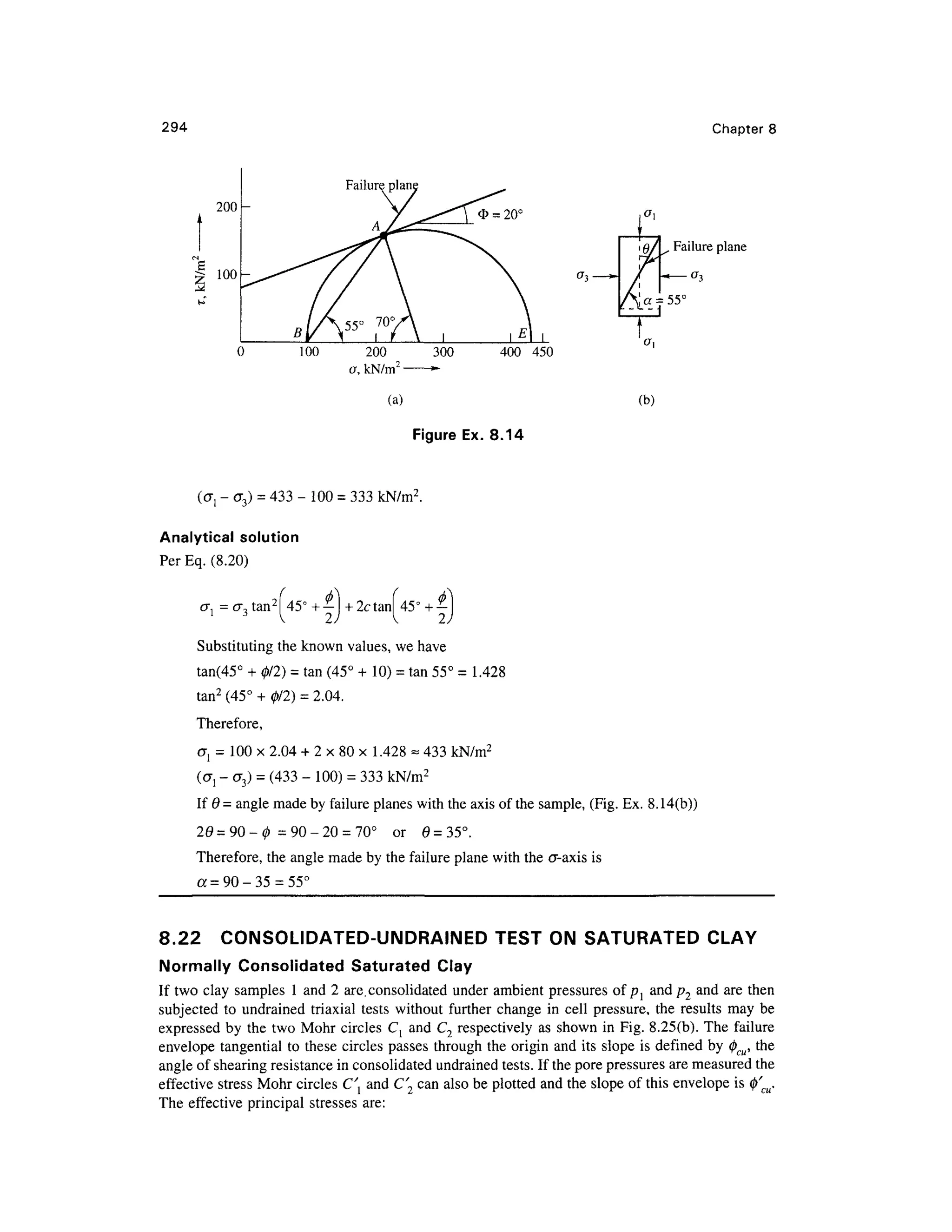
283. 264 Chapte r 8
If the sides of the cylindrical specimen are not acted on by the horizontal pressure <7 3, the load
required t o caus e failur e i s calle d th e unconfme d compressiv e strengt h qu. I t i s obviou s tha t a n
unconfmed compressio n test can be performed onl y on a cohesive soil. According to Eq. (8.20), the
unconfmed compressive strength q i s equal to
<T = a — 2r N f 8 71
u
i y «-] </> (o.Zj)
If 0 = 0, then qu = 2c (8.24a )
or the shear strength
s = c= —(8.24b )
Eq. (8.24b ) show s one o f the simples t way s of determining the shea r strengt h of cohesiv e
soils.
8.9 MOH R CIRCL E O F STRESS
Squaring Eqs. (8.8) and (8.9) and adding, we have
i2 / _ ^ x 2
+ ^ = I " 2 j + *ly (8.25 )
Now, Eq. (8.25) is the equation of a circle whose center has coordinate s
and whose radius is — i/(c7 - c r ) -
2v vy
'
The coordinates of points on the circle represent the normal and shearing stresses on inclined
planes at a given point. The circle is called th e Mohr circle of stress, after Mohr (1 900), who firs t
recognized thi s usefu l relationship . Mohr's metho d provide s a convenient graphical metho d fo r
determining
I . Th e normal and shearing stress on any plane through a point in a stressed body .
2. Th e orientation of the principal planes if the normal and shear stresses on the surface of the
prismatic elemen t (Fig . 8.6 ) ar e known . The relationship s ar e vali d regardles s o f th e
mechanical propertie s o f th e material s sinc e onl y th e consideration s o f equilibriu m are
involved.
If th e surface s o f th e elemen t ar e themselve s principa l planes , th e equatio n fo r th e Moh r
circle of stress may be written as
T + oy -- -
= - y -- ( 8.26)
The center of the circle has coordinates T- 0 , and o=(a{ + (T3)/2, and its radius is (<Jl - (T 3)/2.
Again from Mohr's diagram, the normal and shearing stresses on any plane passing through a point
in a stressed body (Fig. 8.7) may be determined if the principal stresses cr l and (J3 are known. Since
<7j andO" 3 are always known in a cylindrical compression test, Mohr's diagram is a very useful too l
to analyze stresses on failure planes.

284. Shear Strengt h of Soi l 265
8.10 MOH R CIRCL E O F STRESS WHE N A PRISMATI C ELEMEN T
IS SUBJECTED TO NORMA L AND SHEA R STRESSE S
Consider first the case of a prismatic element subjected to normal and shear stresses as in Fig. 8.8(a).
Sign Conventio n
1. Compressiv e stresses are positive and tensile stresses are negative.
2. Shea r stresses are considered a s positive if they give a clockwise moment about a point
above the stressed plane as shown in Fig. 8.8(b), otherwise negative.
The norma l stresse s ar e take n a s absciss a an d th e shea r stresse s a s ordinates . I t i s
assumed the norma l stresses c r , cr an d the shear stress r ( T = T ) acting o n the surface of
x y xy xy yx
the elemen t ar e known . Tw o point s P l an d P 2 ma y no w b e plotte d i n Fig . 8.8(b) , whos e
coordinates are
If the points P} and P2 are joined, the line intersects the abscissa at point C whose coordinates
are [(0,+op/2,0].
Minor principal
> a
i
plane
(a) A prismatic element subjected to normal and shear stresses
(ax + ay)/2
+ ve
(b) Mohr circle of stress
Figure 8.8 Moh r stres s circl e for a general case

285. 266 Chapte r 8
Point O is the origin of coordinates for the center of the Mohr circle of stress. With center C
a circle may now be constructed with radius
This circl e whic h passes throug h points Pl an d P2 i s called th e Mohr circle o f stress. The
Mohr circle intersects the abscissa at two points E and F . The major and minor principal stresses
are ol ( = OF) and cr 3 (= OE) respectively .
Determination o f Norma l an d Shea r Stresse s o n Plan e A A [Fig . 8.8(a) ]
Point P{ o n the circle of stress in Fig. 8. 8(b) represents the state of stress on the vertical plane of the
prismatic element ; similarl y point P2 represent s th e stat e o f stres s o n th e horizonta l plan e o f th e
element. If from point P{ a line is drawn parallel to the vertical plane, it intersects the circle at point PQ
and if from th e point P2 on the circle, a line is drawn parallel to the horizontal plane, this line also
intersects the circle at point PQ . The point PQ so obtained is called the origin of planes or the pole. If
from the pole PQ a line is drawn parallel to the plane AA in Fig. 8.8(a) to intersect the circle at point P3
(Fig. 8.8(b)) then the coordinates o f the point give the normal stress cran d the shear stress Ton plane
AA as expressed by equations 8.8 and 8.9 respectively. This indicates that a line drawn from the pole PQ
at any angle a t o the cr-axi s intersects the circle at coordinates tha t represent the normal and shear
stresses on the plane inclined at the same angle to the abscissa.
Major an d Mino r Principa l Planes
The orientations of the principal planes may be obtained by joining point PQ to the points E and F
in Fig 8.8(b). PQ F is the direction of the major principal plane on which the major principal stres s
dj acts ; similarly PQ E is the direction o f the minor principal plane on which the minor principal
stress<7 3 acts. It is clear from the Mohr diagram that the two planes PQ E and PQ F intersect at a right
angle, i.e., angle EPQ F = 90°.
8.1 1 MOH R CIRCL E O F STRESS FO R A CYLINDRICA L SPECIME N
COMPRESSION TES T
Consider the case of a cylindrical specimen of soil subjected to normal stresses<7 j and<J 3 which are
the major and minor principal stresses respectively (Fig . 8.9 )
From Eqs. (8.14 ) and (8.15), we may write
2 2
Again Eq. (8.27) is the equation of a circle whose center has coordinate s
<7, + CT , (7 , — (J-.
<J = — - -
-and T =
0 and whose radius is
/O /-*^T
(8.27)
2 2
A circle with radius (o{ - cr 3)/2 with its center C on the abscissa a t a distance of (al + cr3)/2
may be constructed a s shown in Fig. 8.9 . This i s the Mohr circle of stress. The majo r and mino r
principal stresses are shown in the figure wherein cr, = OF and<7 3 = OE.
From Fig. 8.8 , we can writ e equations for cf j an d<7 3 and T max as follows
±

286. Shear Strength of Soi l 267
.A
Figure 8.9 Moh r stres s circle for a cylindrical specime n
(8.29)
where Tmax is the maximum shear stress equal to the radius of the Mohr circle.
The origin of planes or the pole PQ (Fig. 8.9) may be obtained as before by drawing lines from
points E and F parallel to planes on which the minor and major principal stresses act . In this case,
the pole PO lies on the abscissa and coincides with the point E.
The normal stress< J and shear stress T on any arbitrary plane AA making an angle a with the
major principal plane may be determined as follows.
From the pole P0 draw a line PQ Pl parallel to the plane AA (Fig. 8.9). The coordinates of the
point Pl giv e the stresses c r and i. From the stress circle we may write
= 2a
cr, + cr, cr, - cr.
- (8.30)
Normal stress a
0° 15 ° 30 ° 45 ° 60 ° 75 ° 90 °
Angle of inclination of plane, a ^
Figure 8.10 Variatio n o f crand r with a

287. 268 Chapte r 8
(j, -cr ,
r= 3
sin2# (8.31 )
Equations (8.30) an d (8.31) are the same as Eqs. (8.14 ) and (8.15) respectively .
It is of interest to study the variation of the magnitudes of normal and shear stresses with the
inclination of the plane.
Eqs. (8.30 ) an d (8.31) are plotted with a a s the abscissa show n in Fig. 8.10 . The following
facts are clear from thes e curves:
1. Th e greates t an d leas t principa l stresse s ar e respectivel y th e maximu m an d minimu m
normal stresse s on any plane through the point in question .
2. Th e maximum shear stress occurs on planes at 45° to the principal planes .
8.12 MOHR-COULOM B FAILURE THEOR Y
Various theories relatin g to the stress condition in engineering materials at the time of failure are
available i n th e engineerin g literature . Each o f thes e theorie s ma y explai n satisfactoril y th e
actions of certain kinds of materials at the time they fail, but no one of them i s applicable t o all
materials. Th e failur e of a soil mas s i s more nearl y i n accordance wit h the tenet s o f the Moh r
theory o f failur e tha n wit h thos e o f an y othe r theor y an d th e interpretatio n o f th e triaxia l
compression tes t depends to a large extent on this fact. The Mohr theory is based on the postulate
that a material will fail when the shearing stress on the plane along which the failure is presumed
to occur is a unique function of the normal stress acting on that plane. The material fails along the
plane only when the angle between the resultant of the shearing stress and the normal stres s is a
maximum, tha t is , wher e th e combinatio n o f norma l an d shearin g stresse s produce s th e
maximum obliquity angle 8.
According to Coulomb's Law , the condition of failure is that the shear stres s
T ^ c + atan^ (8.32 )
In Fig 8.1 l(b) MQN an d MQNl ar e the lines that satisfy Coulomb' s conditio n of failure. If the
stress a t a given point within a cylindrical specimen unde r triaxial compression i s represented b y
Mohr circl e 1 , it may be note d that every plane through this point has a shearing stres s whic h is
smaller than the shearing strength.
For example, if the plane AA in Fig. 8.1 l(a) is the assumed failure plane, the normal and shear
stresses on this plane at any intermediate stage of loading are represented b y point b on Mohr circle
1 where the line PQb is parallel to the plane AA. The shearing stress on this plane is ab which is less
than the shearing strength ac at the same normal stress Oa . Under this stress conditio n there is no
possibility o f failure . O n th e othe r han d i t woul d no t b e possibl e t o appl y th e stres s conditio n
represented b y Mohr stress circle 2 to this sample because it is not possible fo r shearing stresses t o
be greate r tha n the shearin g strength. At the norma l stress Of, th e shearin g stres s o n plane AA is
shown to be fh whic h is greater tha n the shear strength of the materials fg whic h is not possible .
Mohr circle 3 in the figure is tangent to the shea r strengt h line MQN an d MQNj a t points e and e{
respectively. O n the same plane AA at normal stres s Od , the shearing stres s d e is the same a s the
shearing strengt h de . Failur e i s therefor e imminen t on plan e A A at th e norma l stres s O d an d
shearing stress de. The equation for the shearing stress de is
s = de - de'+ e'e = c+ crtan 0 (8.33 )
where 0 is the slope of the line MQN whic h is the maximum angle of obliquity on the failure plane.
The valu e of the obliquity angle can never exceed<5 m = 0, the angle of shearing resistance, withou t
the occurrence of failure. The shear strength line MQN whic h is tangent to Mohr circle 3 is called the

288. Shear Strengt h of Soi l 269
'i /
Rupture
plane Moh r
envelope N
Mohr circle of
rupture
(b)
Figure 8.11 Diagra m presenting Mohr's theory of rupture
Mohr envelope or line of rupture. The Mohr envelope may be assumed as a straight line although it
is curved under certain conditions. The Mohr circle which is tangential to the shear strength line is
called th e Mohr circle o f rupture. Thus the Mohr envelope constitutes a shear diagra m an d is a
graph o f th e Coulom b equatio n fo r shearin g stress . Thi s i s calle d th e Mohr-Coulomb Failure
Theory. The principal objective of a triaxial compression tes t is to establish the Mohr envelope for
the soil being tested. The cohesion and the angle of shearing resistance can be determined from this
envelope. When th e cohesion o f the soil is zero, tha t is, when the soil is cohesionless, th e Mohr
envelope passes through the origin.
8.13 MOH R DIAGRA M FO R TRIAXIAL COMPRESSION TEST A T
FAILURE
Consider a cylindrical specime n o f soi l possessin g bot h cohesion an d frictio n i s subjecte d to a
conventional triaxia l compressio n test . I n th e conventiona l tes t th e latera l pressur e cr 3 i s hel d
constant an d th e vertica l pressur e<T J i s increase d a t a constant rate o f stres s o r strai n unti l th e
sample fails . I f cr l i s the pea k valu e of th e vertica l pressur e a t whic h the sampl e fails , th e tw o
principal stresse s tha t ar e to be use d fo r plotting th e Moh r circl e o f rupture are cr 3 an d or I n
Fig. 8.12 the values of cr { an d<7 3 are plotted on the er-axis and a circle is drawn with (o^ - cr 3) as
diameter. The center of the circle lies at a distance of (<j{ + cr3)/2 from the origin. As per Eq. (8.18),
the soil fails along a plane which makes an angle a, =45° + 0/2 with the major principal plane. In
Fig. 8.12 the two lines PQPl an d PQP2 (where PQ is the origin of planes) are the conjugate rupture
planes. The two lines MQN an d MQN^ draw n tangential to the rupture circle at points Pl an d P2 are
called Mohr envelopes. If the Mohr envelope can be drawn by some other means, the orientation of
the failure planes may be determined.
The result s o f analysi s o f triaxia l compressio n test s a s explaine d i n Sect . 8. 8 ar e no w
presented in a graphical form in Fig. 8.12 . The various information that can be obtained from th e
figure includes
1. Th e angle of shearing resistance 0 = the slope of the Mohr envelope .

289. 270 Chapter 8
A a Mohr envelope
(a, - a3)/2
Figure 8.12 Moh r diagra m fo r triaxia l test at failure fo r c- 0 soil
Rupture
plane
T
c
I
Rupture
plane
0 = 0
0
(a) c = 0
C
(b) 0 = 0
Figure 8.13 Moh r diagra m for soil s wit h c = 0 and = 0
2. Th e apparent cohesion c = the intercept of the Mohr envelope on the T-axis.
3. Th e inclination of the rupture plane = a .
4. Th e angle between the conjugate planes = 2a.
If the soil is cohesionless wit h c = 0 the Mohr envelopes pas s through the origin, and if the
soil is purely cohesive with 0 = 0 the Mohr envelope is parallel to the abscissa. The Mohr envelopes
for these two types of soils are shown in Fig. 8.13.
8.14 MOH R DIAGRA M FO R A DIREC T SHEA R TES T A T FAILUR E
In a direct shear test the sample is sheared alon g a horizontal plane. This indicates that the failure
plane is horizontal. The normal stress don thi s plane is the external vertical load divided by the area
of th e sample . Th e shea r stres s a t failur e i s th e externa l lateral loa d divide d b y th e are a o f th e
sample.
Point Pj on the stress diagram in Fig. 8.14 represents the stress condition on the failure plane.
The coordinates o f the point are
normal stress = <7, shea r stress i- s.

290. Shear Strengt h of Soi l 271
Minor
Plane of rupture
0
t Majo r principal
plane
Figure 8.14 Moh r diagra m for a direct shea r test at failur e
If i t is assume d tha t the Moh r envelop e i s a straight lin e passing throug h th e origi n
(for cohesionles s soi l o r normall y consolidate d clays) , i t follow s tha t th e maximu m
obliquity 8m occurs o n the failure plane and 8m = 0. Therefore th e line OP{ mus t be tangent
to the Mohr circle , an d the circle ma y be constructed a s follows :
Draw Pj C normal t o OPr Poin t C which is the intersection poin t o f the normal wit h the
abscissa i s the center o f the circle. CP { i s the radius of the circle. Th e Mohr circl e ma y no w be
constructed which gives the major and minor principal stresses cr { an d<7 3 respectively .
Since th e failur e i s o n th e horizonta l plane , th e origi n o f plane s P Q ma y b e obtaine d b y
drawing a horizontal line through P{ givin g PQ. PQF and PQE give the directions of the major and
minor principal planes respectively .
Example 8. 1
What is the shearing strength of soil along a horizontal plane at a depth of 4 m in a deposit of sand
having the following properties :
Angle of internal friction, 0 = 35°
Dry unit weight, y d - 1 7 kN/m3
Specific gravity, Gs = 2.7.
Assume the ground water table is at a depth of 2.5 m from th e ground surface. Also find the
change in shear strength when the water table rises to the ground surface .
Solution
The effective vertica l stress at the plane of interest is
<r'=2.50xyd + l.SOx y b
Given yd = 17 kN/m3
and Gs = 2.7
We haver, = 17- = —X9.81
9A9
or lie = 26.5 - 1 7 = 9.49 o r e = —— = 0.56
Therefore, Y b =
l + e 1 +0.56
*9.81 =10.7 kN/m 3

291. 272 Chapter 8
Hence c/ = 2.5 x 1 7 + 1. 5 x 10. 7 = 58.55 kN/m2
Hence, the shearing strength of the sand is
5 = (/ tan 0 = 58.55 x tan 35° = 41 kN/m2
If th e wate r tabl e rises t o th e groun d surface i.e. , by a height of 2. 5 m , th e chang e i n th e
effective stres s will be,
Ao" = yd x 2.5 -Yb* 2. 5 = 17 x 2.5 - 10. 7 x 2.5 = 15.75 kN/m2
(negative)
Hence the decrease in shear strength will be,
= Ac/ tan 35° = 15.7 5 x 0.7 0 = 1 1 kN/m2
Example 8. 2
Direct shea r tests wer e conducted o n a dry sand . The siz e o f the sample s use d fo r th e test s wa s
2 in. x 2 in. x 0.75 in . The test results obtained are given below:
Test No . Norma l loa d Norma l stres s a Shea r forc e Shea r stres s
(Ib) (Ib/ft 2
) a t failur e (Ib ) (Ib/ft 2
)
1 1 5 54 0 1 2 43 2
2 2 0 72 0 1 8 64 8
3 3 0 108 0 2 3 82 8
4 6 0 216 0 4 7 169 2
5 12 0 432 0 9 3 334 8
Determine th e shear
4000-
3000-
c/f
C/3
£ 200 0 -
C/3
j3
1000-
strength parameters cand 0.
^L
S^ A ^" 7 8 °
/
/
y
/
/
1000 2000 3000 4000
Normal stress , a Ib/ft 2
Figure Ex . 8. 2
5000

292. Shear Strengt h of Soi l
Solution
273
The failure shear stresses r^ as obtained from the tests are plotted against the normal stresses a, in
Figure Ex 8.2. The shear parameters from th e graph are: c= 0, 0 = 37.8°.
Example 8. 3
A direct shear test, when conducted on a remolded sample of sand, gave the following observations
at the time of failure: Norma l loa d = 288 N; shear load = 17 3 N. The cross sectiona l are a o f the
sample = 36 cm2
.
Determine: (i) the angle of internal friction, (ii) the magnitude and direction of the principal
stresses in the zone of failure.
Solution
Such problem s ca n be solve d i n tw o ways, namel y graphicall y an d analytically . The analytica l
solution has been lef t as an exercise fo r the students.
Graphical Solutio n
173
(i) Shea r stress T =
= 4.8 N/cm 2
= 48 kN/m2
36
288
Normal stress a =—= 8.0 N / cm2
= 80 k N / m2
36
We know one point on the Mohr envelope. Plot point A (Fig. Ex. 8.3) with coordinates 1 -
48 kN/m2
, and o= 80 kN/m2
. Since cohesion c = 0 for sand, the Mohr envelope OM passes
through the origin. The slop e of OM gives the angle of internal friction(j) = 31° .
(ii) I n Fig. Ex. 8.3, draw line AC normal to the envelope OM cutting the abscissa a t point C.
With C as center, and AC as radius, draw Mohr circle Cl which cuts the abscissa at points B
and D, which gives
120
80
40
Mohr circle C
Major principa l plane
C2
40 F 8 0 C 12 0
a, kN/m2
160 200
Figure Ex. 8. 3

293. 274 Chapte r 8
major principal stress = OB = (J l = 163.5 kN/m 2
minor principal stress = OD = <J 3 = 53.5 kN/m 2
Now, ZACB = 2cc = twic e th e angl e between th e failur e plan e and th e majo r principal
plane. Measurement gives
2a= 121° or a- 60.5 °
Since i n a direct shea r tes t th e failur e plane is horizontal, the angl e mad e b y th e majo r
principal plan e wit h th e horizonta l will be 60.5° . The mino r principa l plane shoul d b e
drawn at a right angle to the major principal plane.
The direction s o f th e principa l planes ma y als o b e foun d by locatin g th e pol e P o. Po i s
obtained by drawing a horizontal line from point A which is parallel to the failure plane in
the direct shear test. Now PE and P(D give the directions of the major and minor principal
planes respectively.
8.15 EFFECTIV E STRESSES
So far, the discussion ha s been based on consideration o f total stresses . I t is to be noted tha t the
strength an d deformation characteristics of a soil can be understood bette r by visualizin g it as a
compressible skeleto n of solid particles enclosing voids. The voids may completely be filled with
water or partly wit h water and air . Shear stresse s are to be carried onl y by the skeleto n o f solid
particles. However , th e tota l norma l stresse s o n an y plan e are , i n general , th e su m o f tw o
components.
Total normal stress = component of stress carried by solid particles
+ pressure in the fluid i n the void space.
This visualizatio n of the distribution o f stresses betwee n soli d an d flui d ha s tw o important
consequences:
1. Whe n a specimen of soil is subjected to external pressure, the volume change of the specimen
is not due to the total normal stress but due to the difference between the total normal stress
and the pressure of the fluid in the void space. The pressure in the fluid is the pore pressure u.
The difference which is called the effective stres s d may now be expressed as
tf = cr-u (8.34 )
2. Th e shea r strengt h o f soils , a s o f al l granula r materials , i s largel y determine d b y th e
frictional force s arisin g during slip at the contacts betwee n th e soil particles . Thes e are
clearly a function o f the component of normal stress carrie d b y the solid skeleton rather
than o f th e tota l norma l stress . Fo r practica l purpose s th e shea r strengt h equatio n o f
Coulomb is given by the expression
s = c
' + (o- U ) tan</)' = c' + a
' tan</)' (8.35 )
where c' = apparent cohesion in terms of effective stresse s
0' =angle of shearing resistance in terms of effective stresses
<7 = total normal pressure to the plane considered
u = pore pressure.
The effectiv e stres s parameter s c' an d 0 ' of a give n sampl e o f soi l ma y b e determine d
provided the pore pressure u developed durin g the shear test is measured. The por e pressure u is
developed whe n th e testin g of th e soi l i s don e unde r undraine d conditions . However , i f fre e

294. Shear Strengt h of Soi l 27 5
drainage takes plac e durin g testing, there will not be any development o f pore pressure . I n such
cases, the total stresses themselves are effective stresses .
8.16 SHEA R STRENGT H EQUATIO N I N TERMS O F EFFECTIV E
PRINCIPAL STRESSE S
The principal stresses ma y be expressed eithe r as total stresses o r as effective stresse s i f the values
of pore pressure are known.
If u is the pore pressure developed durin g a triaxial test, we may write as before
o = o, -u
where a j and<5' 3 are the effective principal stresses. The equation for shear strength in terms
of effective stresse s i s
<7,' — <7o G<— (J-, <J, — (T-.
s = —si n 2a= —si n 2a= —;
co s 0(8.37 )
2 2 2
where 2a= 90° + 0'
Coulomb's equation in terms of effective stresse s is
s = c''+ (<7-u) tan 0'
(7, — (J~.
Therefore, — cos<z> ' = c' + (er-u) tan0'
Since, cr =
2 2
we hav e — co s(/)' = c' H—l
- ta n<f)'
+ — cos(9 0 + 0') ta n 0'- u tan 0'
Simplifying
<7, - cr , , . . . cr , + or, . , O" , -1
. — -.
2 2 2
1 c ' cos$)' + (<73 — «) sin^'
- w s n
or
where (ci j - cr 3) indicate s th e maximum deviator stres s a t failure. Eq (8.38) ma y also b e
expressed i n a different for m as follows by considering effective principal stresse s
1 , , c' cos^' + a
. sin^'
— (<j, -cr, ) , = -
- -
2l 3 f
1-si n
or —

295. 276 Chapte r 8
Simplifying, w e have
(o[ -o'3)f = (o{ + o'3 ) sin(/)' + 2c' cos 0' (8.39 )
8.17 STRESS-CONTROLLE D AN D STRAIN-CONTROLLE D TESTS
Direct shear tests or triaxial compression tests may be carried out by applying stresses or strains at
a particularly known rate. When the stress is applied at a constant rate it is called a stress-controlled
test an d whe n th e strai n is applie d a t a constan t rate i t i s calle d a strain-controlled test. Th e
difference betwee n the two types of tests may be explained with respect t o box shear tests.
In the stress-controlled test [Fig. 8.15(a)] the lateral load Fa which induces shear is gradually
increased unti l complete failur e occurs. Thi s ca n be done b y placin g weights o n a hanger o r by
filling a counterweighte d bucke t o f origina l weigh t W a t a constan t rate . Th e shearin g
displacements are measured by means of a dial gauge G as a function of the increasing load F . The
shearing stress at any shearing displacement, is
where A i s the cross sectional are a o f the sample. A typical shape o f a stress-strain curv e of the
stress-controlled test is shown in Fig. 8.15(a).
A typical arrangement of a box-shear test apparatus for the strain-controlled test is shown in
Fig. 8.15(b) . The shearin g displacements ar e induced and controlled i n such a manner that they
occur at a constant fixed rate. This can be achieved by turning the wheel either by hand or by means
of any electrically operate d motor so that horizontal motion is induced through the worm gear B.
The dial gauge G gives the desired constant rate of displacement. The bottom of box C is mounted
on frictionless rollers D. The shearing resistance offered to this displacement by the soil sample is
measured b y the proving ring E. The stress-strain curves for this type of test have the shape shown
in Fig. 8.15(b).
Both stress-controlled and strain-controlled types of test are used in connection with all the
direct triaxia l and unconfined soi l shea r tests . Strain-controlled tests ar e easier to perform an d
have the advantage of readily giving not only the peak resistance as in Fig. 8.1 5 (b ) but also the
ultimate resistance which is lower than the peak suc h as point b in the same figure, whereas th e
stress controlled gives only the peak values but not the smaller values after the peak is achieved.
The stress-controlled test is preferred only in some special problem s connecte d wit h research.
8.18 TYPE S O F LABORATOR Y TEST S
The laboratory tests on soils may be on
1. Undisturbe d samples, or
2. Remolde d samples .
Further, the tests may be conducted on soils that are :
1 .Full y saturated, or
2. Partiall y saturated.
The type of test to be adopted depend s upon how best we can simulate the field conditions.
Generally speaking, the various shear tests for soils may be classified as follows:

296. Shear Strengt h o f Soi l 277
Dial
gauge
Displacement
_-
(b) Strain controlled
Figure 8.15 Stres s and strain controlle d bo x shear tests
1. Unconsolidated-Undraine d Test s (UU)
The samples are subjected to an applied pressure under conditions in which drainage is prevented,
and then sheared under conditions of no drainage.
2. Consolidated-Undraine d or Quick Tests (CD)
The sample s ar e allowe d t o consolidat e unde r a n applie d pressur e an d the n sheare d unde r
conditions of no drainage.
3. Consolidated-Draine d or Slow Test s (CD)
The samples ar e consolidated a s in the previous test, but the shearing is carried out slowly under
conditions of no excess pressure in the pore space .
The drainage condition of a sample is generally the deciding factor in choosing a particular
type o f tes t i n th e laboratory . Th e purpos e o f carrying ou t a particular tes t i s t o simulat e fiel d
conditions a s fa r a s possible . Becaus e o f th e hig h permeabilit y o f sand , consolidatio n occur s
relatively rapidl y an d is usually completed durin g the application o f the load. Tests o n sand are
therefore generall y carried out under drained conditions (drained or slow test).
For soils other than sands the choice of test conditions depends upon the purpose for which
the shear strength i s required. The guiding principle is that drainage conditions o f the test should
conform as closely as possible t o the conditions under which the soils will be stressed i n the field.
Undrained or quick tests ar e generally use d for foundations on clay soils , sinc e during the
period of construction only a small amount of consolidation will have taken place and consequently
the moisture content will have undergone little change. For clay slopes o r cuts undrained tests are
used both for design an d for the investigation of failures.
Consolidated-undrained test s are used where changes in moisture content are expected to take
place due to consolidation before the soil is fully loaded. An important example is the condition known
as "sudden drawdown" such as that occurs in an earth dam behind which the water level is lowered at

297. 278 Chapte r 8
a faster rate than at which the material of the dam can consolidate. In the consolidated-undrained tests
used in this type of problem, the consolidation pressures are chosen to represent the initial conditions
of the soil, and the shearing loads correspond to the stresses called into play by the action of sudden
drawdown.
As already stated, drained tests are always used in problems relatin g to sandy soils. In clay
soils drained tests are sometimes used in investigating the stability of an earth dam, an embankment
or a retaining wall after a considerable interval of time has passed.
Very fine sand, silts and silty sands also have poor drainage qualities. Saturated soils of these
categories ar e likely to fail in the field under conditions similar to those under which consolidated
quick tests are made.
Shearing Tes t Apparatu s fo r the Variou s Types o f Test s
The various types of shear tests mentioned earlier may be carried out either by the box shear test or
the triaxial compression test apparatus. Tests that may be made by the two types of apparatus are:
Box Shea r Test Apparatus
1. Undraine d and consolidated- undrained tests on clay samples only.
2. Draine d or Slow tests on any soil.
The box shear test apparatus is not suited for undrained or consolidated-undrained test s on
samples other than clay samples, because the other soils are so permeable that even a rapid increase
of the stresses i n the sample may cause at least a noticeable change of the water content.
Triaxial Compression Test Apparatus
All types of tests can conveniently be carried out in this apparatus.
8.19 SHEARIN G STRENGT H TEST S O N SAND
Shear tests on sand may be made when the sand is either in a dry state or in a saturated state. No test
shall be made when the soil is in a moist state a s this state exists onl y due to apparent cohesio n
between particle s whic h would be destroye d whe n it i s saturated. The result s o f shea r test s on
saturated samples are almost identical with those on the same sand at equal relative density in a dry
state except that the angle 0 is likely to be 1 or 2 degrees smaller for the saturated sand.
The usua l typ e o f tes t use d fo r coars e t o mediu m san d i s th e slo w shea r test . However ,
consolidated undraine d tests may be conducted on fine sands, sandy silts etc. which do not allow
free drainage under changed stress conditions. If the equilibrium of a large body of saturated fin e
sand i n a n embankment is disturbed by rapid drawdown of th e surfac e of a n adjoinin g body of
water, the change in water content of the fill lags behind the change in stress.
In all the shearing tests on sand, only the remolded samples are used as it is not practicable to
obtain undisturbed samples. The soil samples are to be made approximately to the same dry density
as it exists in-situ and tested either by direct shear or triaxial compression tests.
Tests on soils are generally carried out by the strain-controlled type apparatus. The principal
advantage of this type of test on dense san d is that its peak-shear resistance, as well as the shea r
resistances smalle r than the peak, can be observed and plotted.
Direct Shea r Tes t
Only th e drained or the slo w shear test s on sand may be carried ou t by using the box shea r tes t
apparatus. The box is filled wit h sand to the required density. The sample is sheared at a constant

298. Shear Strengt h of Soi l 279
vertical pressure a. The shear stresses are calculated at various displacements of the shear box. The
test is repeated with different pressure s<7 .
If th e sampl e consist s o f loos e sand , th e shearin g stres s increase s wit h increasin g
displacement until failure occurs. If the sand is dense, the shear failure of the sample is preceded by
a decrease o f the shearing stress from a peak value to an ultimate value (also known as residual
value) lower than the peak value.
Typical stress-strain curves for loose and dense sands are shown in Fig. 8.16(a).
The shear stress of a dense sand increases from 0 to a peak value represented by point a, and
then gradually decreases and reaches an ultimate value represented by point b. The sample of sand
in a dense state is closely packed and the number of contact points between the particles are more
than in the loose state. The soil grains are in an interlocked state. As the sample is subjected to shear
stress, th e stres s ha s t o overcom e th e resistanc e offere d b y th e interlocke d arrangemen t o f th e
particles. Experimental evidence indicates that a significant percent of the peak strength is due to
the interlocking of the grains. In the process of shearing one grain tries to slide over the other and
the voi d rati o of th e sampl e whic h is th e lowes t a t the commencemen t o f th e tes t reache s th e
maximum value at point a, in the Fig 8.16(a). The shear stress also reaches the maximum value at
this level . An y furthe r increas e o f strai n beyon d thi s poin t i s associate d wit h a progressiv e
disintegration of the structure of the sand resulting in a decrease i n the shear stress . Experienc e
shows that the change in void ratio due to shear depends on both the vertical load and the relative
density of the sand. At very low vertical pressure, the void ratio at failure is larger and at very high
pressure it is smaller than the initial void ratio, whatever the relative density of the sand may be. At
Peak value
Dense sand
b ultimat e value
Displacement
(a) Shear stress vs displacement
0
Dense sand
Loose sand
(b) Volume change
Normal stress, a
(c) Shear strength vs normal stres s
Figure 8.16 Direc t shea r test o n sand

299. 280 Chapte r 8
Table 8.1 Typica l value s of 0 and (j) u fo r granula r soil s
Types of soi l
Sand: rounded grains
Loose
Medium
Dense
Sand: angular grains
Loose
Medium
Dense
Sandy gravel
0 deg
28 to 30
30 to 35
35 to 38
30 to 35
35 to 40
40 to 45
34 to 48
0u deg
26 to 30
30 to 35
33 to 36
intermediate values of pressure, the shearing force causes a decrease in the void ratio of loose sand
and an increase i n the void ratio of dense sand. Fig 8.16(b) shows how the volume of dense sand
decreases u p t o a certai n valu e o f horizonta l displacemen t an d wit h furthe r displacemen t th e
volume increases , wherea s i n th e cas e o f loose san d th e volum e continues to decreas e wit h an
increase in the displacement. In saturated san d a decrease of the void ratio is associated with an
expulsion of pore water, and an increase with an absorption of water. The expansion of a soil due to
shear a t a constant valu e of vertica l pressure i s called dilatancy. At som e intermediat e stat e o r
degree of density in the process of shear, the shear displacement does not bring about any change in
volume, that is, density. The density of sand at which no change in volume is brought about upon
the applicatio n o f shea r strain s i s calle d th e critical density. Th e porosit y an d voi d rati o
corresponding t o th e critica l densit y are calle d th e critical porosity an d th e critical void ratio
respectively.
By plottin g the shea r strength s corresponding to the state of failure i n the differen t shea r test s
against the normal pressure a straight line is obtained for loose sand and a slightly curved line for dense
sand [Fig . 8.16(c)] . However , fo r al l practica l purposes , th e curvatur e for th e dens e san d ca n b e
disregarded an d an average line may be drawn. The slopes of the lines give the corresponding angles of
friction 0 of the sand. The general equation forthe lines may be written as
s = <J tan(f)
For a given sand, the angle 0 increases wit h increasing relative density. For loose san d it is
roughly equal to the angle of repose, defined as the angle between the horizontal and the slope of a
heap produced by pouring clean dry sand from a small height. The angle of friction varie s with the
shape of the grains. Sand samples containing well graded angular grains give higher values of 0 as
compared to uniformly graded san d with rounded grains. The angl e of friction</ > for dense sand at
peak shear stress is higher than that at ultimate shear stress. Table 8.1 gives some typical values of
0 (at peak) and 0 M (at ultimate).
Triaxial Compression Test
Reconstructed sand samples at the required density are used for the tests. The procedure of making
samples shoul d be studie d separately (refe r to any book o n Soil Testing). Tests o n sand ma y be
conducted either in a saturated state or in a dry state. Slow or consolidated undraine d tests may be
carried out as required.
Drained o r Slow Test s
At least three identical samples havin g the same initial conditions are to be used. For slow test s
under saturated conditions the drainage valve should always be kept open. Each sample should be

300. Shear Strengt h of Soi l 281
': v•••:..-y<; A
jv:,:^-V^
-• ' -
i .* • '
'- '' •" '
• v
••*». • '- x ' ' ' « ' "
••> " "•.. , ." ' • ••> '
(a) Dense san d (b ) Loose sand
Figure 8.17 Typica l shape s of dens e and loose sands a t failur e
Strain
(a) Stress-strain curves for three samples at dense state
Mohr
envelope
(b) Mohr envelope
Figure 8.18 Moh r envelop e fo r dens e sand

301. 282 Chapte r 8
tested unde r different constan t all-round pressures for example, 1 , 2 and 3 kg/cm2
. Each sampl e is
sheared t o failure by increasing the vertical load at a sufficiently slo w rate to prevent any build up
of excess por e pressures .
At an y stag e o f loadin g th e majo r principa l stres s i s th e all-roun d pressur e<7 3 plu s th e
intensity of deviator stress (o{ - cr 3). The actually applied stresses are the effective stresses i n a slow
test, that is<7 } = aandO" 3 = <r'3, Dense sample s fai l along a clearly define d rupture plane wherea s
loose sand samples fail along many planes which result in a symmetrical bulging of the sample. The
compressive strengt h o f a sampl e i s define d a s th e differenc e betwee n th e majo r an d mino r
principal stresses a t failure (GI - <T 3),,. Typical shapes of dense and loose sand samples at failure are
shown in Fig. 8.17 .
Typical stress-strai n curves for three sample s i n a dense stat e and the Mohr circles fo r these
samples a t peak strengt h are shown in Fig. 8.18.
If the experiment is properly carried out there will be one common tangen t to all these thre e
circles an d this will pass through the origin. This indicates that the Mohr envelope i s a straight line
for sand and the sand has no cohesion. The angle made by the envelope with the a-axis is called the
angle o f internal friction. The failure planes fo r each o f these sample s ar e shown in Fig. 8.18(b) .
Each of them make an angle a with the horizontal which is approximately equal to
a = 45° + 0/2
From Fig . 8.18(b) an expression for the angle of internal friction ma y be written as
- (J 3 (T j / <7 3 - 1
(840)
{Q
-™}
Example 8. 4
Determine th e magnitude of the deviator stress if a sample of the same sand with the same void ratio
as given in Ex. 8.3 was tested in a triaxial apparatus with a confining pressure o f 60 kN/m 2
.
Solution
In the case of a triaxial test on an identical sample of sand as given in Ex. 8.3, us e the same Moh r
envelope O M (Fig . Ex . 8.3) . No w th e poin t F o n th e absciss a give s th e confinin g pressur e
<73 = 60 kN/m2
. A Mohr circle C2 may now be drawn passing through point F and tangential to the
Mohr envelope OM . The point E gives the major principal stress<J } fo r the triaxial test.
Now cr j = O E = 188 kN/m2
,<7 3 = 60 kN/m2
Therefore a l - <7 3 = 188 - 6 0 =128 kN/m
2
= deviator stres s
Example 8. 5
A consolidated draine d triaxial test was conducted on a granular soil. At failure cr'/o ^ = 4.0. The
effective mino r principal stress a t failur e wa s 10 0 kN/m 2
. Comput e 0 ' an d th e principal stres s
difference a t failure.
Solution
-j -1 4- 1
3 +1 4 + 1
The principal stress difference at failure is
sin<z$' = —; ~ = ~
= 0.6 o r 6' - 37°
cr,7cr3 + 14 + 1

302. Shear Strengt h o f Soi l 28 3
,
= <^ —-1 = 100(4-l ) = 300kN/m2
^
Example 8. 6
A draine d triaxia l tes t o n san d wit h cr' 3 = 315 0 lb/ft 2
gav e (ala f
^)f= 3.7 . Comput e (a )
(b) (o-j - 0-3)^ , and (c) $'.
Solution
Therefore, o{ = 3.1(Tf
3 = 3.7 x3 15
0 = 1 1,655 lb/ft 2
(b) (<T ! - o-3)/ = (0-; -crp
/ = 11,655 -3150 = 8505 lb/ft2
l 3.7- 1
OT
Example 8. 7
Assume th e tes t specime n i n Ex . 8. 6 wa s sheare d undraine d at the sam e tota l cel l pressur e o f
3150 lb/ft2
. The induced excess pore water pressure at failure u, was equal to 1470 lb/ft2
. Compute:
(a) o f
(b) (cr , - 0 3)f
(c) 0 i n terms of total stress,
(d) th e angle of the failure plane a,
Solution
(a) and (b): Since the void ratio after consolidation would be the same for this test as for Ex. 8.6,
assume §' is the same.
a'
cr, - a-, ), =cr( , — L
-1
7 J /
-
As before (
°3/ =
^3/ ~ «/ = 3150 -1470 = 1680 lb/ft 2
So (ff l - cr 3 )f = 1680 (3.7 -
1) = 4536 lb/ft 2
a(f = (ffl -0 3)f + &'3f = 4536 + 1680 = 6216 lb/ft 2
(c) sin<z> f, , = -
1
2 . =
= 0.59 o r 0 tn1. =36.17°
<"totai 621 6 + 1470 tota l
(d) From Eq. (8.18)

303. 284 Chapte r 8
af = 45° + — = 45° + — = 62.5°
7
2 2
where 0'is taken from Ex . 8.6.
Example 8. 8
A saturate d specime n o f cohesionles s san d wa s teste d unde r draine d condition s i n a triaxia l
compression tes t apparatus and the sample failed at a deviator stress of 482 kN/m2
and the plane of
failure mad e a n angle of 60° with the horizontal . Find th e magnitude s o f th e principal stresses .
What would be the magnitudes of the deviator stress and the major principal stres s a t failure fo r
another identical specimen of sand if it is tested under a cell pressure of 200 kN/m2
?
Solution
Per Eq. (8.18), the angle of the failure plane a is expressed a s equal to
Since a = 60°, w e have 0 = 30°.
From Eq . (8.40), si n ^ = —1
with 0 = 30°, and (7, - cr 3 = 482 kN/m2
. Substituting we have
o-j - <J 3 48 2
°"i +
^3 =
~7 ~ ~ • on o = 964 kN/m2
(a )
1 J
sin^z ) si n 30
cr, - cr 3 -482 kN/m2
(b )
solving (a) and (b) we have
ol = 723 kN/m2
, an d <J 3 = 241 kN/m2
For the identical sample
0 = 30°,<T 3 = 200 kN/m2
From Eq. (8.40), we have
cr, - 200
Sin30
°=^7^
Solving for<T J we have a l = 600 kN/m2
and (cr , - cr 3) = 40 0 kN/m2
8.20 UNCONSOLIDATED-UNDRAINE D TES T
Saturated Cla y
Tests on saturated clay may be carried out either on undisturbed or on remolded soi l samples. The
procedure o f the test is the same i n both cases. A series of samples (a t least a minimum of three)
having the same initia l condition s are tested unde r undrained conditions. Wit h ay th e all-round
pressure, actin g on a sample under conditions of no drainage, the axial pressure is increased until
failure occurs at a deviator stress (<7 , - (7 3). From the deviator stress, the major principal stress cr, is
determined. I f the othe r sample s ar e tested i n the sam e wa y but wit h different values o f cr 3, it is

304. Shear Strengt h of Soi l 285
found tha t for al l types o f saturate d clay , the deviator stres s a t failure (compressive strength ) is
entirely independent of the magnitude of cr 3 as shown in Fig. 8.19. The diameters of all the Mohr
circles are equal and the Mohr envelope is parallel to the cr-axis indicating that the angle of shearing
resistance 0 U = 0 . Th e symbo l 0 U represent s th e angl e o f shearin g resistanc e unde r undrained
conditions. Thus saturated clays behave as purely cohesive materials with the following properties:
(8.41)
where cu is the symbol used for cohesion under undrained conditions. Eq. (8.41) holds true for the
particular case of an unconfined compression tes t in which<7 3 = 0. Since this test requires a very
simple apparatus, i t is often used , especiall y fo r field work , as a ready mean s o f measuring th e
shearing strength of saturated clay, in this case
q
= —!L
, wher e (8.42)
Effective Stresses
If during the test, pore-pressures ar e measured, the effective principal stresse s ma y be written as
<j( = CT j - U
(8.43)
where u is the pore water pressure measured during the test. The effective deviato r stress at failure
may be written as
Eq. (8.44) shows that the deviator stress is not affected by the pore water pressure. As such the
effective stres s circle is only shifted from the position of the total stress circle as shown in Fig. 8.19.
Partially Saturate d Cla y
Tests o n partiall y saturate d cla y ma y b e carrie d ou t eithe r o n undisturbe d or o n remolde d soi l
samples. All the samples shall have the same initial conditions before the test, i.e., they should possess
the same water content and dry density. The tests are conducted in the same wa y as for saturated
samples. Each sampl e i s tested unde r undrained conditions wit h different all-roun d pressures o~ 3.
T
C
u
A.
Effective stres s circl e
Total stress circl e
Figure 8.19 Moh r circl e for undraine d shea r test on saturated cla y

305. 286 Chapter 8
Figure 8.2 0 Moh r circl e for undraine d shea r tests o n partially saturate d cla y soil s
Total stress
circle
Figure 8.21 Effectiv e stres s circle s fo r undraine d shea r tests on partiall y saturate d
clay soil s
Mohr circle s fo r three soi l sample s an d the Mohr envelop e ar e shown in Fig. 8.20 . Thoug h al l the
samples had the same initial conditions, the deviator stress increases with the increase in the all-round
pressureo~ 3 as shown in the figure. This indicates that the strength of the soil increases with increasing
values of o~3. The degree of saturation also increases with the increase in o~3. The Mohr envelope which
is curved at lower values ofo~3 becomes almost parallel to the o*-axis as full saturation is reached. Thus
it is not strictly possibl e t o quote single values for the parameters c u and § u for partially saturated
clays, but over any range of normal pressure cr; encountered in a practical example, the envelope can
be approximated by a straight line and the approximate values of cu and 0H can be used in the analysis.
Effective Stresses
If the pore pressures ar e measured during the test, the effective circle s can be plotted as shown in
Fig. 8.2 1 and the parameters c' and 0' obtained. The envelope to the Mohr circles, when plotted in
terms of effective stresses, i s linear.
Typical undraine d shear strengt h parameter s fo r partially saturated compacte d sample s ar e
shown in Table 8.2 .
8.21 UNCONFINE D COMPRESSIO N TEST S
The unconfme d compressio n tes t is a special cas e of a triaxial compression tes t in which the all-
round pressureo" 3 = 0 (Fig. 8.22) . Th e test s are carried ou t only o n saturated sample s whic h can
stand without any lateral support. The test, is, therefore, applicable to cohesive soil s only. The test

306. Shear Strengt h of Soi l 28 7
Table 8.2 Probabl e undrained shear strength parameters for partially saturated soil s
Types o f soil
Sand with clay binder
Lean silty clay
Clay, moderate plasticity
Clay, very plastic
cu (tsf)
0.80
0.87
0.93
0.87
4>u
23°
13°
9°
8°
c'(tsf)
0.70
0.45
0.60
0.67
0'
40°
31°
28°
22°
is an undrained test and is based on the assumption that there is no moisture loss during the test. The
unconfmed compression test is one of the simplest and quickest tests used for the determination of
the shear strength of cohesive soils. These tests can also be performed in the field by making use of
simple loading equipment.
Figure 8.22 Unconfine d compression test equipment (Courtesy : Soiltest )

307. 288 Chapte r 8
Any compressio n testin g apparatus wit h arrangement fo r strai n contro l ma y b e use d fo r
testing the samples . The axial load u may be applied mechanically or pneumatically.
Specimens of height to diameter ratio of 2 are normally used for the tests. The sampl e fail s
either by shearing on an inclined plane (if the soil is of brittle type) or by bulging. The vertical stress
at any stage of loading is obtained by dividing the total vertical load by the cross-sectional area. The
cross-sectional are a of the sample increases with the increase in compression. Th e cross-sectiona l
area A at any stage of loading of the sample may be computed on the basic assumption that the total
volume of the sample remains the same. That is
AO/IQ = A h
where A Q, hQ = initial cross-sectional area and height of sample respectively.
A,h = cross-sectional area and height respectively at any stage of loading
If Ah is the compression of the sample, the strain is
A/z
£
~ ~j~~ sinc e A/ z =h
0- h, we may write
AO/ZQ = A(/ZO - A/z )
Therefore, A = -j^-= ^
^ = ^
(8.45 )
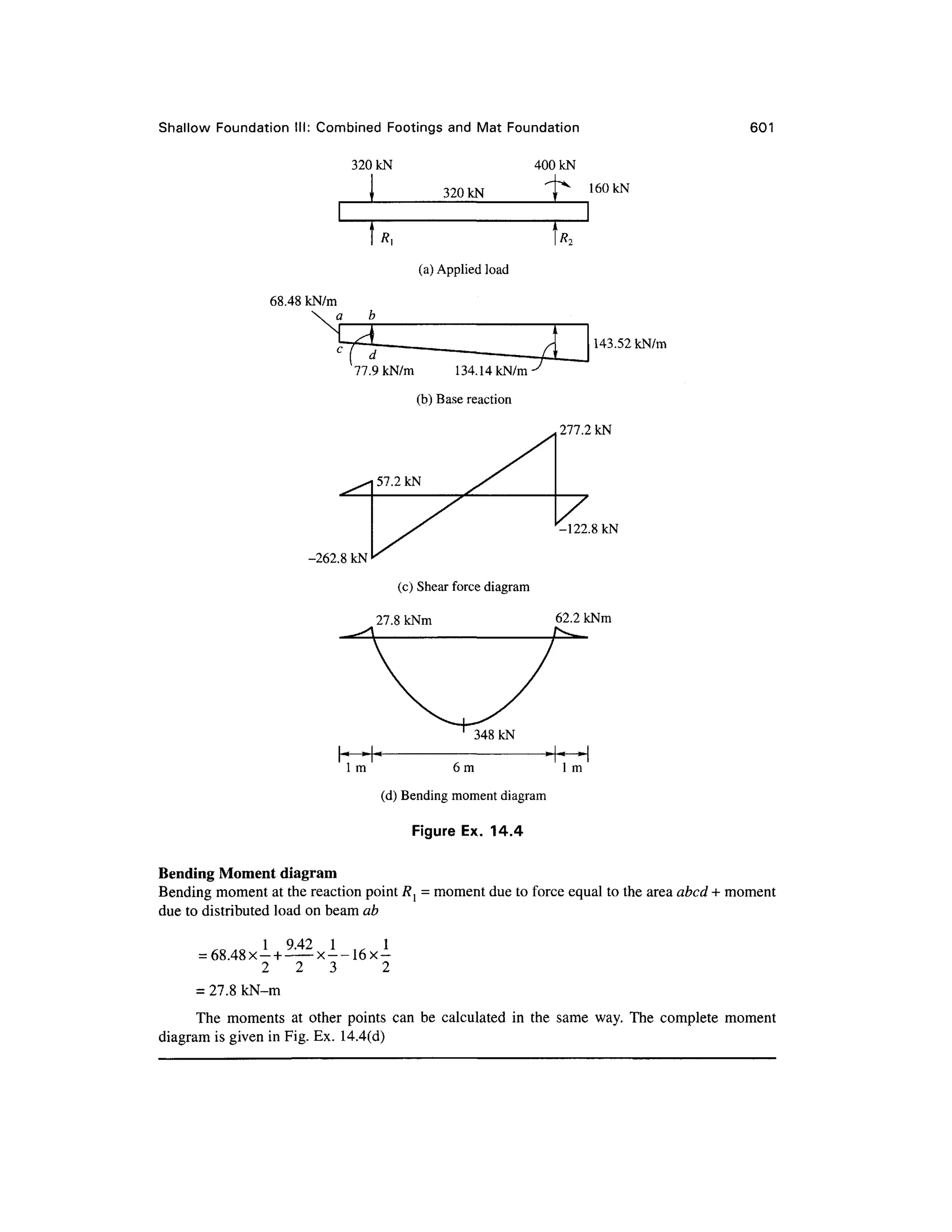
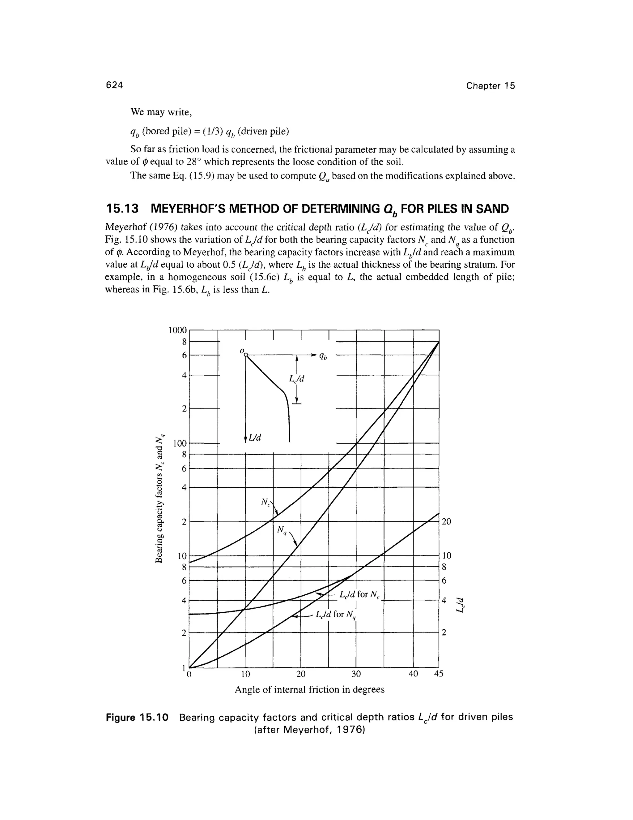
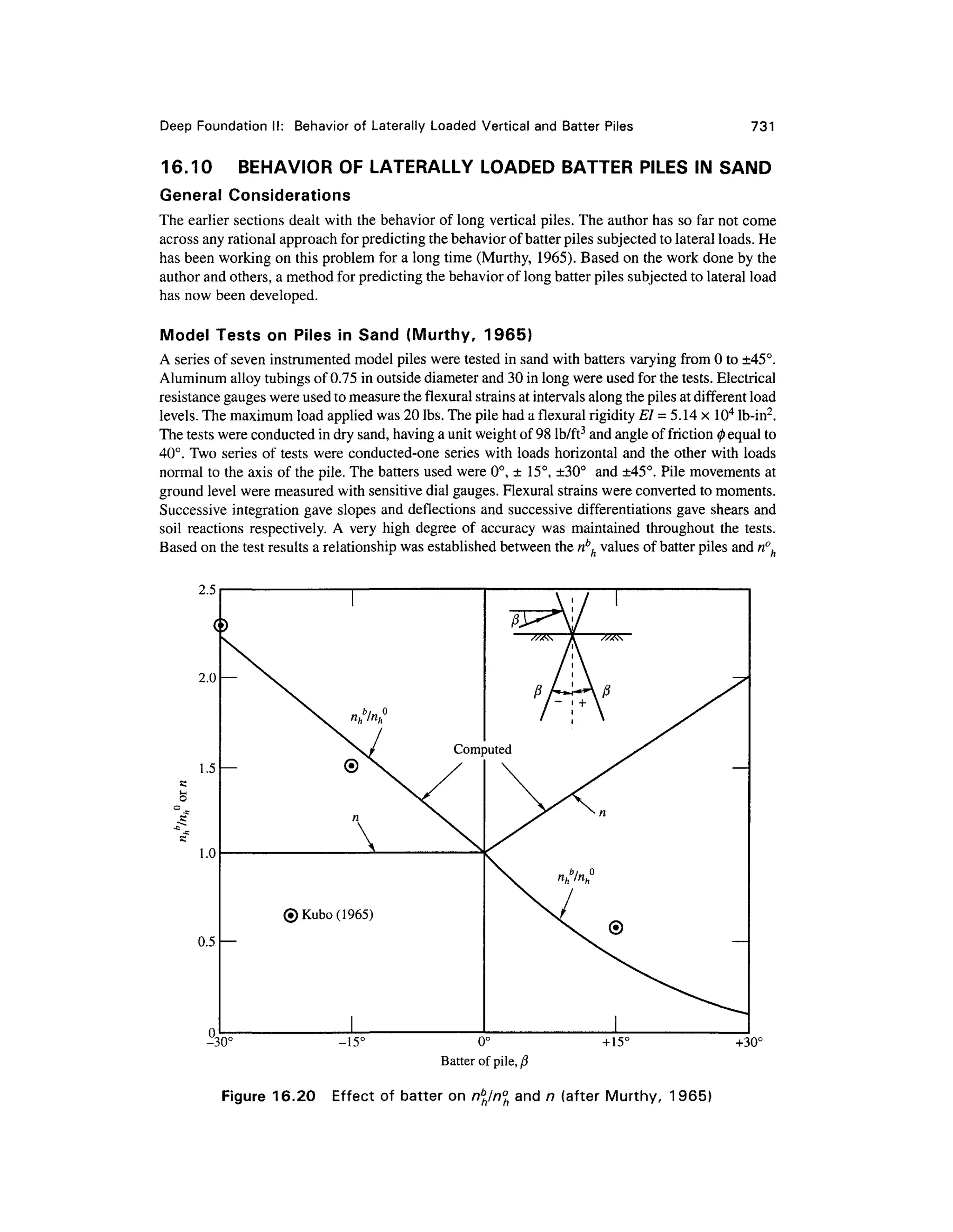
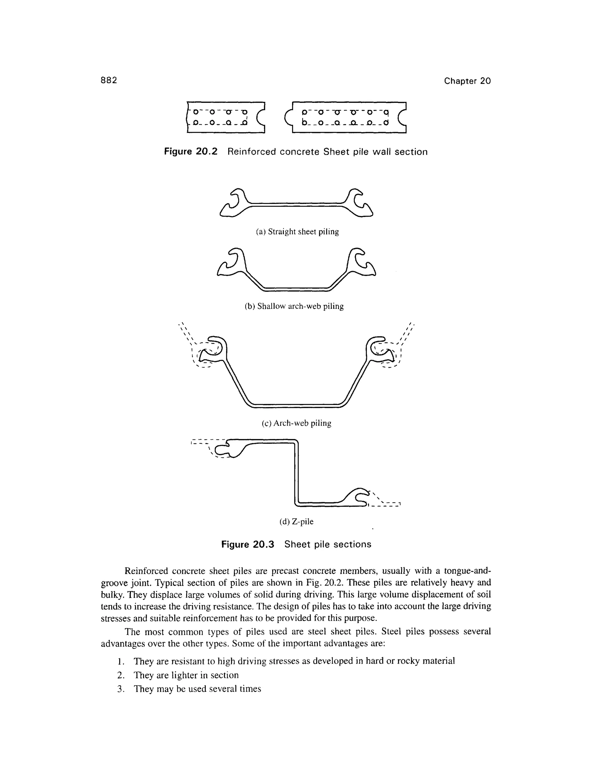
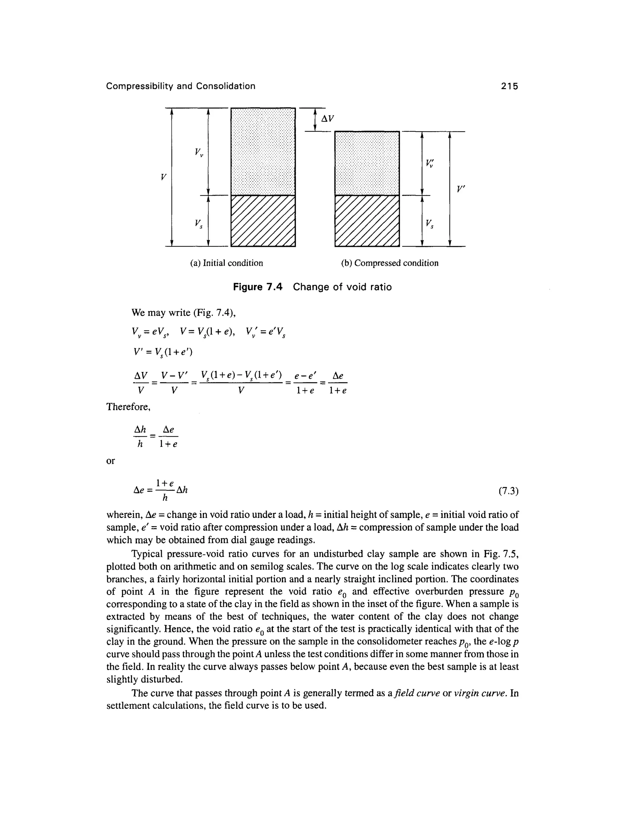
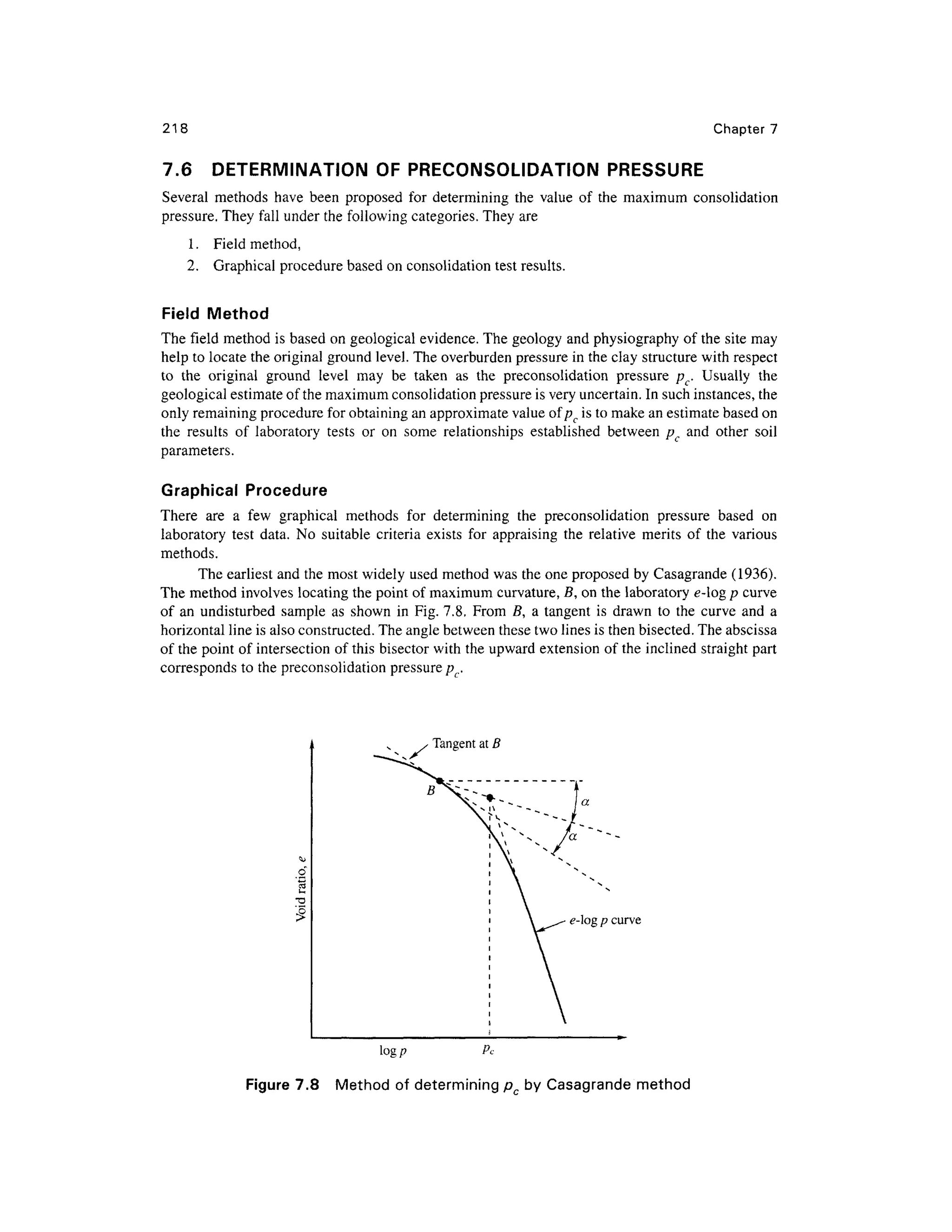
The average vertical stress at any stage of loading may be written as
P P(l-e]
A A ()
(8.46)
where P is the vertical load at the strain e.
Using the relationship given by Eq. (8.46) stress-strain curves may be plotted. The peak value
is taken as the unconfined compressiv e strength qti, that is
( f f
i ) f
=
V u (8-47 )
The unconfine d compression test (UC ) i s a specia l cas e o f th e unconsolidated-undrained
(UU) triaxial compression test (TX-AC). The only difference between the UC test and UU test is
that a total confining pressure under which no drainage was permitted was applied in the latter test.
Because of the absence of any confining pressure in the UC test, a premature failure through a weak
zone may terminate an unconfined compression test. For typical soft clays, premature failure is not
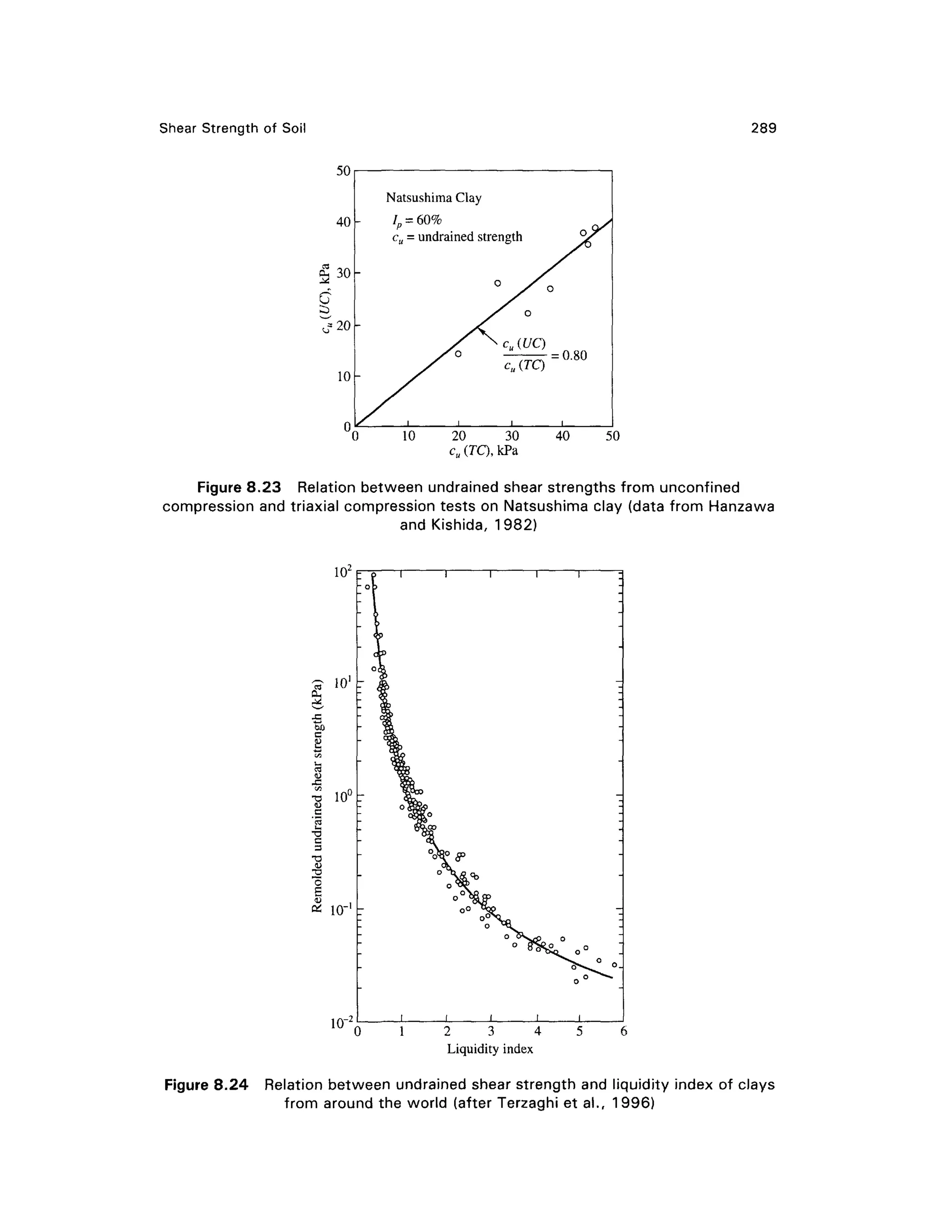
likely to decrease th e undrained shear strength by more than 5%. Fig 8.23 show s a comparison of
undrained shear strength values from unconfine d compression tests and from triaxia l compression
tests on soft-Natsushima cla y from Toky o Bay. The properties o f the soil are :
Natural moisture content w = 80 to 90%
Liquid limit w,= 10 0 to 110 %
Plasticity index /; = 60%
There is a unique relationship between remolded undraine d shear strength and the liquidity
index, / , as shown in Fig. 8.24 (after Terzaghi et al., 1996). This plot includes soft clay soil and silt
deposits obtaine d from differen t part s of the world.

308. Shear Strengt h of Soi l 289
50
40
§ 3 0
: ? 2 0
10
Natsushima Clay
Ip = 60%
cu = undrained strengt h
cu(UQ
°
= 0.80
0 1 0 2 0 3 0 4 0 5 0
cu (TQ, kPa
Figure 8.23 Relatio n between undrained shear strengths from unconfine d
compression and triaxial compression tests on Natsushima clay (data from Hanzawa
and Kishida, 1982)
102
10'
M
r v
•0 10 °
2
"o
10-
10" 2 3 4
Liquidity inde x
Figure 8.24 Relatio n between undrained shear strength an d liquidity index of clays
from around the world (afte r Terzagh i et al., 1996 )

309. 290 Chapte r 8
Example S.9
Boreholes revea l tha t a thin layer of alluvial silt exists at a depth of 50 ft below th e surface of the
ground. The soil above this level has an average dry unit weight of 96 lb/ft 3
an d an average wate r
content of 30%. The water table is approximately at the surface. Tests on undisturbed samples give
the followin g data : c u = 100 8 lb/ft 2
, 0 M = 13° , cd = 861 lb/ft 2
,(j) d = 23°. Estimat e th e shearin g
resistance of the silt on a horizontal plane (a) when the shear stress builds up rapidly, and (b) when
the shear stress builds up very slowly.
Solution
Bulk unit weight y t = yd (1 + w) = 96 x 1.3 = 124.8 lb/ft 3
Submerged uint weight y b = 124.8- 62.4 = 62.4 lb/ft 3
Total normal pressure at 50 ft depth = 50 x 124. 8 = 6240 lb/ft2
Effective pressur e at 50 ft depth = 50 x 62.4 = 3120 lb/ft 2
(a) For rapid build-up, use the properties of the undrained state and total pressure.
At a total pressure of 6240 lb/ft 2
shear strength, s = c + crtan</ > = 100 8 + 6240 tan 13 ° = 2449 lb/ft2
(b) For slow build-up, use effective stress propertie s
At an effective stres s of 3120 lb/ft 2
,
shear strength = 861 + 3120 tan 23° = 2185 lb/ft 2
Example 8.1 0
When a n undraine d triaxial compression tes t wa s conducte d o n specimen s o f claye y silt , th e
following results were obtained:
Specimen No. 1
cr3(kN/m2
) 1 7 4 4 5 6
<T! (kN/m2
) 15 7 20 4 22 5
M (kN/m2
) 1 2 2 0 2 2
Determine th e value s o f shea r parameter s considerin g (a ) tota l stresse s an d (b ) effective
stresses.
Solution
(a) Total stresses
For a solution with total stresses, dra w Mohr circles Cr C2 and C3 for each of the specimens
using the corresponding principa l stresses a { an d cr 3.
Draw a Mohr envelop e tangen t to these circle s a s shown i n Fig. Ex . 8.10 . No w from th e
figure
c- 48 kN/m2
, 0= 15°

310. Shear Strengt h of Soi l 291
120
80
40
c = 48 kN/m2
c' = 46kN/m2
40 80 12 0
a, kN/m2
»
Figure Ex. 8.1 0
200 240
(b) With effective stresse s
The effective principa l stresse s ma y be found b y subtracting the pore pressures u from th e
total principal stresses as given below.
Specimen No .
cr'3 = (CT3 - u) kN/m 2
o = (CTJ - w ) kN/m2
1
5
145
2
24
184
3
34
203
As befor e dra w Moh r circle s C', , C" 2 an d C" 3 fo r eac h o f th e specimen s a s show n i n
Fig. Ex. 8.10. Now from th e figure
c' = 46 kN/m2
, $'= 20°
Example 8.1 1
A soi l ha s a n unconfine d compressive strengt h o f 12 0 kN/m2
. I n a triaxia l compressio n tes t a
specimen of the same soil when subjected to a chamber pressure of 40 kN/m2
failed at an additional
stress of 160 kN/m2
. Determine:
(i) The shear strength parameters of the soil, (ii) the angle made by the failure plane with the
axial stress in the triaxial test.
Solution
There is one unconfined compression tes t result and one triaxial compression tes t result. Hence two
Mohr circles, Cp and C2 may be drawn as shown in Fig. Ex. 8.11. For Mohr circle Cr cr3 = 0 and
CTj = 120 kN/m2
, an d fo r Moh r circle C 2, O 3 = 40 kN/m2
an d a { = (40 + 160 ) = 200 kN/m 2
. A
common tangent to these two circles is the Mohr envelope which give s
(i) c = 43 kN/m2
and 0 = 19°
(ii) For the triaxial test specimen, A is the point of tangency for Mohr circle C2 an d C is the
center of circle C 2. The angle made by AC with the abscissa is equal to twice the angle between the
failure plane and the axis of the sample = 26. From Fig. Ex. 8.11, 26 = 71 °and 6 = 35.5°. The
angle made by the failure plane with the er -axis is a = 90°-35.5° = 54.5°.

311. 292 Chapter 8
80 120 160 20 0
o, kN/m2
•
Figure Ex . 8.11
Example 8.12
A cylindrical sampl e o f saturated clay 4 cm in diameter an d 8 cm high was tested i n an unconfined
compression apparatus . Find the unconfined compression strength , if the specimen faile d at an axial
load of 360 N, when the axial deformation was 8 mm. Find the shear strength parameters i f the angle
made by the failure plane with the horizontal plane was recorded a s 50°.
Solution
Per Eq. (8.46), the unconfined compression strengt h of the soil is given by
where P =
A = = 12.56 cm2
, = —= 0.
1
8
50 100 15 0
a, kN/m2
0 = 10 °
200 250
Figure Ex. 8.12

312. Shear Strengt h of Soi l 29 3
Therefore a , = 360(1
~°-1)
= 25.8 N/ cm2
= 258kN/m 2
1
12.5 6
Now 0 = 2a - 90° (Refer to Fig. 8.12) where a = 50°.Therefore 0 = 2 x 50 -90° =10°.
Draw the Mohr circle as shown in Fig. Ex. 8.12 (a3 = 0 and o~j = 258 kN/m2
) and from th e
center C of the circle, draw CA at 2a =100°. At point A, draw a tangent to the circle. The tangent is
the Mohr envelope which gives
c = 106 kN/m2
, an d 0=10°
Example 8.13
An unconfmed cylindrica l specimen o f clay fails under an axial stress of 5040 lb/ft2
. The failure
plane was inclined at an angle of 55° to the horizontal. Determine the shear strength parameters of
the soil.
Solution
From Eq. (8.20),
<rl=(T3N</>+2cjN^, wher e ^ = tan2
45 ° +
|
since< T = 0, we have
= 2c tan ^45° + -
, wher e ^ = 5040 lb/ft2
(a )
From Eq. (8.18), the failure angle a is
o
a = 45 + — , sinc e a = 55°, w e have
2
From Eq. (a),
c =
2tan45°-4 2tan55
°
2
Example 8.1 4
A cylindrical sample of soil having a cohesion of 80 kN/m2
and an angle of internal friction of 20°
is subjected to a cell pressure of 100 kN/m2
.
Determine: (i) the maximum deviator stress ((jj- <73) at which the sample will fail, and (ii) the
angle made by the failure plane with the axis of the sample.
Graphical solution
<73 = 100 kN/m2
, 0 = 20°, and c = 80 kN/m2
.
A Mohr circle and the Mohr envelope can be drawn as shown in Fig. Ex. 8.14(a). The circle
cuts the cr-axi s at B (= <7 3), and a t E (= o^). Now <7 j = 433 kN/m 2
, and<7 3 = 10 0 kN/m2
.

313. 294 Chapter 8
200
100
100 20 0 30 0
a, kN/m 2
» •
(a)
400 45 0
(b)
Figure Ex. 8.1 4
(<7, - cr 3) = 433 -10 0 = 333 kN/m2
.
Analytical solution
Per Eq. (8.20)
or, = a, tan2
45 ° +— +2cta n 45 ° + —
1 3
I 2 ) I 2 .
Substituting the known values, we have
tan(45° + 0/2) = tan (45° + 10) = tan 55° = 1.42 8
tan2
(45° + 0/2) = 2.04.
Therefore,
<7, = 100 x 2.04 + 2 x 80 x 1.42 8 « 433 kN/m2
(CTj - <J 3) = (433 - 100 ) = 333 kN/m2
If 6 = angle made by failure planes with the axis of the sample, (Fig. Ex. 8.14(b))
29 = 90 -0 = 90 -2 0 =70° o r 6 =35°.
Therefore, th e angle made by the failure plane with the cr-axis is
a- 9 0 -35 = 55°
8.22 CONSOLIDATED-UNDRAINE D TEST O N SATURATED CLAY
Normally Consolidate d Saturated Cla y
If tw o cla y samples 1 and 2 are.consolidated under ambient pressures o f pl an d p2 an d are then
subjected t o undraine d triaxial tests withou t further chang e i n cel l pressure , th e result s ma y b e
expressed b y th e tw o Moh r circles C L an d C 2 respectively a s shown in Fig. 8.25(b). The failur e
envelope tangentia l to these circles passe s throug h the origin and its slope i s defined by 0 CM, the
angle of shearing resistance in consolidated undrained tests. If the pore pressures are measured the
effective stres s Mohr circles C and C'2 can also be plotted and the slope of this envelope i s 0'cu<
The effectiv e principa l stresses are :

314. Shear Strengt h of Soi l 295
Axial strain Axia l strain
(a) Variation of (a - a3) and u with axial strain
[- " 2 H
(b) Mohr envelope
Figure 8.25 Normall y consolidated clay under undraine d triaxial test
p P2 P^=Pa
Total stress
circle
Effective
stress circle
(^3)1 (^3) 2 (^3) 3
Figure 8.26 Consolidated-undraine d tests on saturated overconsolidated clay

315. 296 Chapter 8
° =
°~
where ul an d w2 are the pore water pressures for the samples 1 and 2 respectively.
It i s a n experimenta l fact tha t the envelope s t o th e tota l an d effectiv e stres s circle s ar e
linear. Fig. 8.25(a) shows the nature of the variation on the deviator stress (<7 j - <7 3) and the pore
water pressur e u in the specimen during the test with the axial strain. The por e wate r pressur e
builds up during shearing with a corresponding decrease in the volume of the sample.
Overconsolidated Cla y
Let a saturated sample 1 be consolidated under an ambient pressure pa an d then allowed to swell
under the pressure pr A n undrained triaxial test is carried ou t on this sample under the all-round
pressure p(= <T 31). Another sample 2 is also consolidated under the same ambient pressure pa an d
allowed to swell under the pressure p2(=<7 32). An undrained triaxial test is carried out on this sample
under th e same all-roun d pressure p2. Th e tw o Mohr circles ar e plotted an d the Mohr envelop e
tangential to the circles is drawn as shown in Fig. 8.26. The shear strength parameters are cu and 0CU.
If pore water pressure is measured, effective stress Moh r circles ma y be plotted a s shown in the
figure. The strength parameters for effective stresse s are represented by c'and §'.
8.23 CONSOLIDATED-DRAINE D SHEA R STRENGT H TES T
In drained triaxial tests the soil is first consolidated under an ambient pressure pa and then subjected to
an increasing deviator stress until failure occurs, the rate of strain being controlled in such a way that
at no time is there any appreciable pore-pressure in the soil. Thus at all times the applied stresses are
effective, an d whe n the stresse s a t failure ar e plotted i n the usua l manner, the failur e envelope is
directly expressed i n terms of effective stresses . Fo r normally consolidated clay s and for sands the
envelope is linear for normal working stresses and passes throug h the origin as shown in Fig. 8.27 .
The failur e criterion fo r suc h soil s i s therefor e th e angl e o f shearin g resistanc e i n th e draine d
condition 0d.
The drained strength is
-(o-1-ff3)/=- . -sin (8.48)
Eq. (8.48) is obtained from Eq. (8.38)
Figure 8.27 Draine d tests on normally consolidate d cla y sample s

316. Shear Strengt h of Soi l 297
Peak /O.C . clay
Ultimate
N.C. clay
Axial strain
3
I
D,
X
U
CX
o
u
O.C. clay
Axial strain
N.C. clay
(a) Variation of (a - a3) with axial strain
O.C. clay
Q
N.C. clay
Normal stress, o
(b) Mohr envelope
Figure 8.28 Draine d tests o n overconsolidated clays
For overconsolidated clays, the envelope intersects the axis of zero pressure at a value cd. The
apparent cohesion i n the drained test and the strength are given by the expression.
(8.49)
1-sini
The Mohr envelope for overconsolidated clay s is not linear as may be seen in Fig. 8.28(b). An
average line is to be drawn within the range of normal pressure crn. The shear strength parameters cd
and(j) d ar e referred t o this line.
Since the stresses in a drained test are effective, it might be expected that a given(f) d woul d be
equal t o 0 ' a s obtaine d fro m undraine d test s wit h pore-pressur e measurement . I n normall y
consolidated clays and in loose sands the two angles of shearing resistance are in fact closely equa l
since the rate of volume change in such materials at failure in the drained test is approximately zer o
and there is no volume change throughout an undrained test on saturated soils. But in dense sands
and heavily overconsolidated clays there is typically a considerable rate of positive volume chang e
at failure in drained tests, and work has to be done not only in overcoming the shearing resistanc e
of the soils, but also in increasing the volume of the specimen agains t the ambient pressure. Yet in

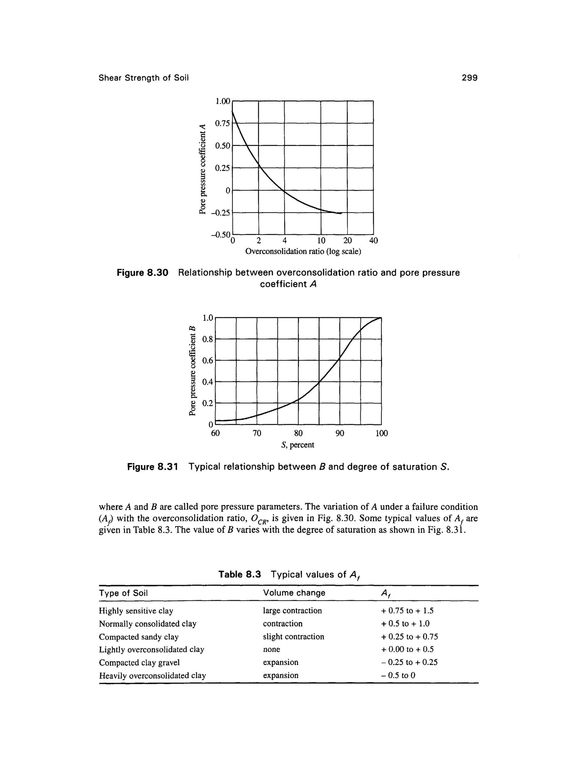
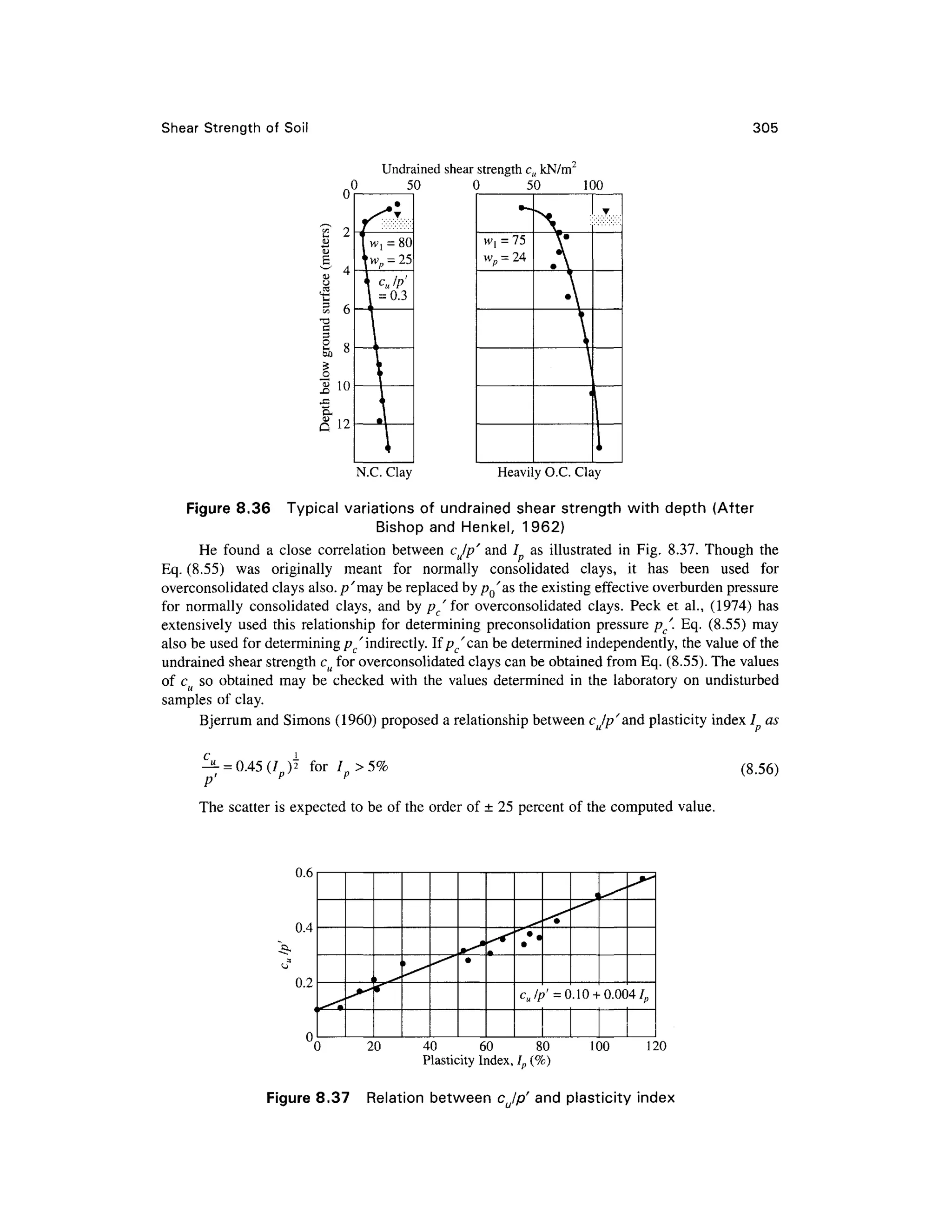
317. 298 Chapter 8
undrained tests on the sam e soils, the volume change is zero and consequently(j) d fo r dense sand s
and heavily overconsolidated clays is greater than 0'. Fig. 8.28(a) shows the nature of variation of
the deviator stres s with axial strain. During the application o f the deviator stress, the volume of the
specimen gradually reduces for normally consolidated clays. However, overconsolidated clays go
through some reduction of volume initially but then expand.
8.24 POR E PRESSURE PARAMETERS UNDER UNDRAINE D
LOADING
Soils in nature are at equilibrium under their overburden pressure. If the same soil is subjected to an
instantaneous additional loading, there will be development of pore pressure if drainage is delayed
under the loading. The magnitude of the pore pressure depends upo n the permeability of the soil,
the manner of application of load, the stress history of the soil, and possibly many other factors. If
a load is applied slowl y and drainage takes place with the application of load, there will practically
be no increase o f pore pressure. However, if the hydraulic conductivity of the soil is quite low, and
if the loading is relatively rapid, there will not be sufficient time for drainage to take place. In such
cases, there will be an increase in the pore pressure in excess of the existing hydrostatic pressure. It
is therefore necessary man y times to determine or estimate the excess pore pressure for the various
types o f loadin g conditions . Por e pressure parameter s ar e use d t o express th e response o f por e
pressure t o changes i n total stres s under undrained conditions. Values of the parameters ma y be
determined i n the laboratory an d can be used t o predict pore pressure s i n the field under similar
stress conditions.
Pore Pressur e Parameter s Under Triaxia l Test Condition s
A typical stress application on a cylindrical element of soil under triaxial test conditions is shown in
Fig. 8.29 (Adj > A<73). AM is the increase in the pore pressure without drainage. From Fig. 8.29, w e
may write
AM3 = 5A<73, Awj = Afi(Acr1 - Acr 3), therefore,
AM = AMj + AM3 = #[A<73 + /4(A(Tj - Acr 3)]
or A M =BAcr3 + A(Aer, - A<r 3)
where, A = AB
for saturate d soils B = 1, so
(8.50)
(8.51)
Aw = A< 7 - A<73)
IACT,
(8.52)
ACT,
A<73 A<7 3
(ACT, - ACT 3)
ACT, AM,
ACT, ACT, (ACT, - ACT 3)
Figure 8.29 Exces s water pressur e unde r triaxia l tes t conditions

318. Shear Strengt h of Soi l 299
Pore
pressure
coefficient
A
3
O
O
O
O
»
-
/>
K
>
N
J
0
»
^-
J
C
D
Lr
t
O
<-f
i
O
<-
t
C
v
,*-^
0 2 4 1 0 2 0 4 0
Overconsolidation ratio (log scale)
Figure 8.30 Relationshi p between Overconsolidatio n ratio and pore pressure
coefficient A
OQ
£
pressure
£
1.0
o
bo
60 70 80
S, percent
90 100
Figure 8.31 Typica l relationship betwee n B and degree of saturatio n S.
where A and B are called pore pressure parameters. The variation of A under a failure condition
(A,) wit h th e Overconsolidation ratio, O CR, is given in Fig. 8.30 . Som e typica l values of A, are
given in Table 8.3. The value of B varies with the degree of saturation as shown in Fig. 8.31.
Table 8.3 Typica l values of Af
Type o f Soi l
Highly sensitive clay
Normally consolidated cla y
Compacted sand y clay
Lightly overconsolidated cla y
Compacted cla y gravel
Heavily overconsolidated cla y
Volume chang e
large contraction
contraction
slight contractio n
none
expansion
expansion
At
+ 0.75 to + 1.5
+ 0.5 to + 1.0
+ 0.25 to + 0.75
+ 0.00 to + 0.5
- 0.2 5 to +0.2
5
- 0.5 to 0

319. 300 Chapte r 8
8.25 VAN E SHEA R TEST S
From experienc e i t has been found that the vane test can be used a s a reliable in-sit u test fo r
determining the shear strengt h of soft-sensitive clays. It is in deep beds o f such material that
the van e test is most valuable , for the simple reaso n tha t there is at present n o other metho d
known b y whic h th e shea r strengt h o f thes e clay s ca n b e measured . Repeate d attempts ,
particularly i n Sweden, have failed to obtain undisturbe d samples fro m depths o f more than
about 1 0 meter s i n normall y consolidate d clay s o f hig h sensitivit y eve n usin g th e mos t
modern for m o f thin-walle d piston samplers . I n thes e soil s th e van e i s indispensable . Th e
vane should be regarded a s a method t o be use d unde r the following conditions:
1. Th e clay is normally consolidated and sensitive.
2. Onl y the undrained shear strength is required.
It has been determined that the vane gives results similar to those obtained from unconfme d
compression test s on undisturbed samples.
The soil mass should be in a saturated condition if the vane test is to be applied. The vane test
cannot be applied to partially saturated soils to which the angle of shearing resistance i s not zero.
Description of the Van e
The vane consists of a steel rod having at one end four small projecting blades or vanes parallel t o
its axis, and situated at 90° intervals around the rod. A post hole borer i s first employed t o bore a
hole up to a point just above the required depth. The rod is pushed or driven carefully until the vanes
are embedded a t the required depth. At the other end of the rod above the surface of the ground a
torsion head is used to apply a horizontal torque and this is applied at a uniform speed of about 0.1°
per se c unti l th e soi l fails , thu s generating a cylinder of soil. The area consists o f the periphera l
surface o f the cylinde r and the tw o round ends. The first moment o f thes e area s divided b y th e
applied moment gives the unit shear value of the soil. Fig. 8.32(a) gives a diagrammatic sketc h of a
field vane .
Determination o f Cohesio n o r Shear Strengt h o f Soi l
Consider th e cylinder of soil generated b y the blades o f the vane when they are inserted int o the
undisturbed soil in-situ and gradually turned or rotated about the axis of the shaft or vane axis. The
turning moment applied at the torsion head above the ground is equal to the force multiplied by the
eccentricity.
Let the force applied = P eccentricity (lever arm) = x units
Turning moment = Px
The surface resisting the turning is the cylindrical surface of the soil and the two end faces of
the cylinder.
Therefore,
resisting moment = (2nr x L x cu x r + Inr2
x cu x 0.67r) = 2nr2
cu(L + 0.67r)
where r = radius of the cylinder and cu the undrained shear strength.
At failure the resisting moment of the cylinder of soil is equal to the turning moment applie d
at the torsion head.
Therefore, P x = 2/rr2
cu(L + 0.67r)
Px
(8>53)

320. Shear Strengt h of Soi l 301
1. Straingauge for
reading torqu e
2. Rotation indicato r
3. 8-in casing with side fins for
anchoring torque assembl y
4. Torque rod
5. A-rod for applying torque to
vane. Made up in 5-ft lengths
(a)
Torque ring
5° graduations
1.0
0.8
0.6
0.4
20 4 0 6 0 8 0
Plasticity index, lp
100 120
6. BX casing for housing
torque rod and A rod
7. Vane rod
8. BX-casing-point containing
bearing and water seals for vane rod
9. Vane varying sizes
2 in dia by 4 in
3 in dia by 6 in
4 in dia by 8 in
(b)
Figure 8.32 Van e shear test (a ) diagrammatic sketch of a field vane, (b ) correction
factor i (Bjerrum , 1973)
The standar d dimension s o f fiel d vane s as recommende d b y AST M (1994) ar e give n in
Table 8.4.
Some investigators believe that vane shear tests in cohesive soil gives a values of the shear
strength abou t 1 5 per cen t greater than in unconfmed compressio n tests . There ar e other s wh o
believe that vane tests give lower values.
Table 8.4 Recommende d dimensions o f field vanes (ASTM, 1994 )
Casing siz e
AX
BX
NX
Height,
mm (L )
76.2
101.6
127.0
Diameter,
mm (d )
38.1
50.8
63.5
Blade thickness
mm
1.6
1.6
3.2
Diameter of ro d
mm
12.7
12.7
12.7

321. 302 Chapter 8
0.6
0.4
0.2
Based on
Bjerrum curves
00
20 40 60 80 100
Figure 8.33 Undraine d shea r strengths from field vane test s o n inorganic sof t
clays an d silts (afte r Tavenas and Leroueil, 1987 )
Bjerrum (1973) back computed a number of embankment failures on soft clay and concluded
that the vane shear strength tended to be too high. Fig. 8.32(b) gives correction factors for the field
vane test as a function o f plasticity index, / (Lad d et al., 1977) . We may write
cu (field) = IJLC U (vane ) (8.54 )
where i is the correction facto r (Fig. 8.32b).
Fig. 8.3 3 giv e relationships between plasticity index / an d cjp' wher e cu is the undrained
shear strength obtained by field vane and//the effective overburde n pressure. This plot is based on
comprehensive tes t dat a compiled o f Tavenas an d Leroueil (1987) . Necessar y correctio n factor s
have been applie d to the data as per Fig. 8.32 (b) before plotting.
8.26 OTHE R METHODS FO R DETERMINING UNDRAINE D SHEAR
STRENGTH O F COHESIVE SOILS
We have discussed in earlier sections three methods for determining the undrained shear strength of
cohesive soils. They are
1. Unconfme d compressio n test
2. U U triaxial test
3. Van e shear test
In this section two more methods are discussed. The instruments used for this purpose are
1. Torvan e (TV )
2. Pocke t penetrometer (PP)
Torvane
Torvane, a modification of the vane, is convenient for investigating the strength of clays in the walls
of tes t pit s i n th e fiel d o r fo r rapi d scannin g o f th e strengt h o f tub e o r spli t spoo n samples .
Fig 8.34(a) gives a diagrammatic sketch of the instrument. Figure 8.34(b) gives a photograph of the
same. The vane s ar e presse d t o their full dept h int o the cla y belo w a flat surface , whereupo n a
torque i s applie d throug h a calibrate d sprin g unti l th e cla y fail s alon g th e cylindrica l surfac e

322. Shear Strengt h of Soi l 303
LJUULJU
(a)
Figure 8.34 Torvan e shear device (a) a diagrammatic sketch , an d (b ) a photograp h
(Courtesy: Soiltest)
circumscribing the vanes and simultaneously along the circular surface constituting the base of the
cylinder. The value of the shear strength is read directly from the indicator on the calibrated spring.
Specification for three sizes of vanes are given below (Holtz et al., 1981 )
Diameter (mm )
19
25
48
Height o f van e (mm )
3
5
5
Maximum shear strength (kPa)
250
100 (standard)
20
Pocket Penetrometer
Figure 8.3 5 show s a pocket penetromete r (Holt z et al. , 1981 ) whic h can b e use d t o determin e
undrained shea r strengt h o f cla y soil s bot h i n th e laborator y an d i n th e field . Th e procedur e
consists in pushing the penetrometer directl y into the soil and noting the strength marked on the
calibrated spring .

323. 304 Chapte r 8
Figure 8.3 5 Pocke t penetromete r (PP) , a hand-held devic e whic h indicate s
unconfined compressiv e strengt h (Courtesy : Soiltest , USA )
8.27 TH E RELATIONSHI P BETWEE N UNDRAINE D SHEA R
STRENGTH AN D EFFECTIV E OVERBURDE N PRESSURE
It ha s bee n discusse d i n previou s section s tha t th e shea r strengt h i s a functio n o f effectiv e
consolidation pressure . I f a relationshi p betwee n undraine d shea r strength , c u, an d effectiv e
consolidation pressure/?'can be established, we can determine cu if //is known and vice versa. If a
soil stratum in nature is normally consolidated th e existing effective overburden pressurepQ'can be
determined fro m th e know n relationship . Bu t i n overconsolidate d natura l cla y deposits , th e
preconsolidation pressur e /?/i s unknown whic h has to be estimated b y any one of the availabl e
methods. If there is a relationship between pc'and cu, cu can be determined fro m the known value of
pc". Alternatively, if cu is known, p/can be determined. Som e o f the relationships between c u and
p' ar e presente d below . A typica l variatio n of undraine d shea r strengt h wit h dept h i s show n i n
Fig. 8.3 6 fo r bot h normall y consolidate d an d heavil y overconsolidate d clays . Th e highe r shea r
strength as shown in Fig. 8.36(a) for normally consolidated clays close to the ground surface is due
to desiccation o f the top layer of soil.
Skempton (1957 ) establishe d a relationship which may be expressed a s
^- =0.10 + 0.004 /„ (8.55 )

324. Shear Strengt h of Soi l 305
Undrained shear strength cu kN/m
2
50 0 5 0 10 0
N.C. Clay Heavily O.C. Cla y
Figure 8.36 Typica l variation s o f undraine d shea r strength with depth (Afte r
Bishop an d Henkel, 1962 )
He foun d a clos e correlatio n betwee n cjp' an d I a s illustrate d i n Fig . 8.37 . Thoug h th e
Eq. (8.55) wa s originall y mean t fo r normall y consolidate d clays , i t ha s bee n use d fo r
overconsolidated clay s also, //may be replaced by p^as the existing effective overburden pressure
for normall y consolidate d clays , an d b y /?c'for overconsolidate d clays . Pec k e t al. , (1974 ) ha s
extensively use d thi s relationshi p for determinin g preconsolidation pressur e pc'. Eq . (8.55 ) ma y
also be used for determining^'indirectly. If p^can be determined independently, the value of the
undrained shear strength c u for overconsolidated clay s can be obtained fro m Eq. (8.55). The values
of c s o obtaine d ma y b e checke d wit h the value s determined i n th e laborator y o n undisturbe d
samples o f clay.
Bjerrum and Simons (1960 ) proposed a relationship between cjp'and plasticit y index / a s
^• = 0.45(7,)* fo r I p>5%
The scatte r i s expected t o be of the order of ± 25 percent of the computed value .
(8.56)
u.o
0.4
0.2
A
I
^
i
1 _^
f
t .
^
^
•
^
_^
'••
"*9
J
^
^
^
cu Ip' = 0.10 + 0.004 I p
20 4 0 6 0 8 0
Plasticity Index , I p (% )
100 12 0
Figure 8.37 Relatio n between cjp' an d plasticity inde x

325. 306 Chapter 8
Another relationshi p expresse d by them is
- = 0.1 8 for / > 0 . 5 (8.57)
where I { i s the liquidity index. The scatter is found to be of the order of ± 30 percent.
Karlsson and Viberg (1967) proposed a relationship as
— = 0.005w, fo r w, > 20 percen t
P'
(8.58)
where vl is the liquid limit in percent. The scatter is of the order of ± 30 percent .
The enginee r ha s t o us e judgment while selecting an y on e o f th e form s o f relationship s
mentioned above .
cjp' Rati o Relate d to Overconsolidatio n Rati o Pc'lp0'
Ladd and Foott (1974) presented a non-dimensional plot (Fig. 8.38) giving arelationship between a non-
dimensional factor jV,and Overconsolidation ratio OCR. Figure 8.38 is based on direct simple shear tests
carried out on five clays from different origins. The plot gives out a trend but requires further investigation.
The non-dimensiona l factor Nf i s defined as
(8.59)
oc
where pQ' = existing overburden pressure
OC = overconsolidate d
NC = normally consolidate d
From th e plot in Fig. 8.38 the shear strengt h c o f overconsolidated cla y can be determine d
if pQ'and (cJp 0')NC ar e known.
.2 3 -
Upper limit
Average line
Lower limi t
4 6 8
Overconsolidation ratio
10 12
Figure 8.38 Relationshi p betwee n N f and Overconsolidation rati o OCR (Ladd and
Foott, 1974 )

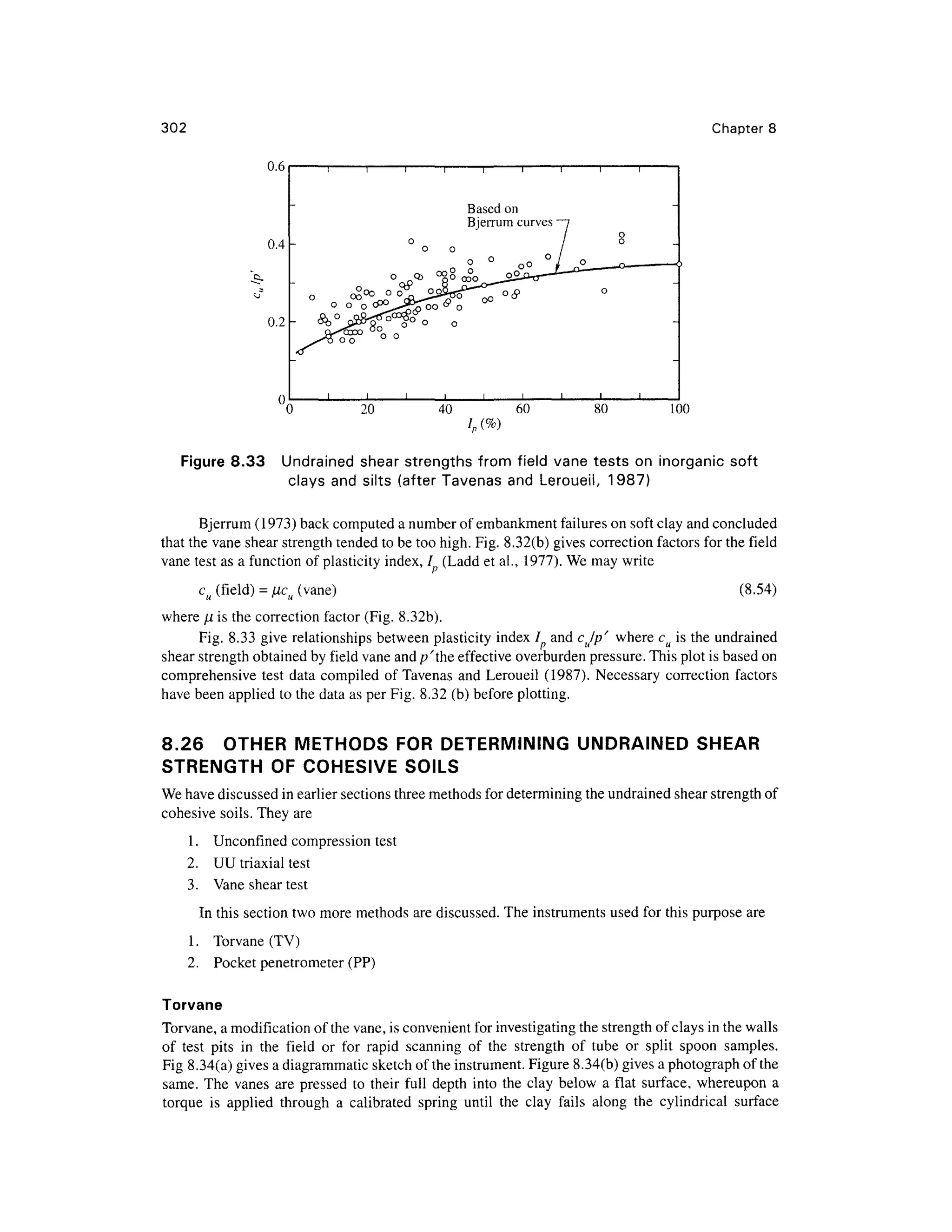
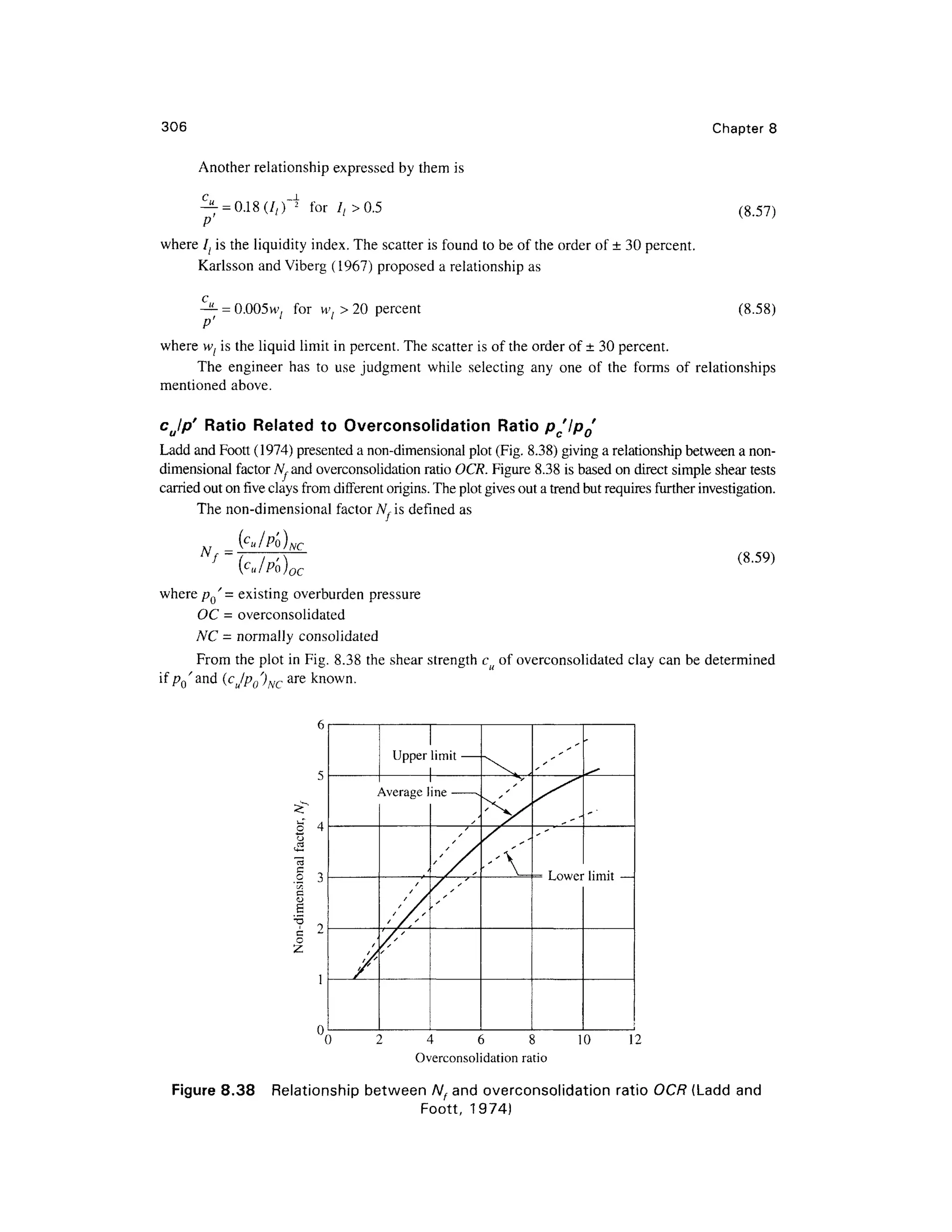
326. Shear Strengt h of Soi l 30 7
Example 8.15
A normall y consolidate d cla y wa s consolidate d unde r a stres s o f 315 0 lb/ft2
, the n sheare d
undrained in axial compression. The principal stress difference at failure was 2100 lb/ft2
, an d the
induced por e pressur e a t failur e wa s 184 8 lb/ft2
. Determin e (a ) th e Mohr-Coulom b strengt h
parameters, i n term s o f bot h tota l an d effectiv e stresse s analytically , (b ) comput e ((T,/cr 3), and
(<7/
1/cr/
3),, and (c) determine the theoretical angle of the failure plane in the specimen.
Solution
The parameters required are: effective parameters c' and 0', and total parameters c and 0.
(a) Given <T3/= 3150 lb/ft 2
, and (<TJ - a 3)f= 2100 lb/ft2
. The total principal stress at failure alf
is obtained from
fflf= (CT j - aj f+ <7 3/ =2100 + 3150 =5250 lb/ft 2
Effective o /
1/= alf- u f= 5250 - 184 8 = 3402 lb/ft 2
°V =
cr3/- "/= 3150 - 184 8 = 1302 lb/ft2
Now cr j = <7 3 tan2
(45° + 0/2) + 2c tan (45° + 0/2
)
Since the soil is normally consolidated, c = 0. As such
---tan2
(45°
-tan (45 or
T * I * " 1 210
° ' I 2 1 0 0
1, 1 Co
Total 0 =sin ]
-
= sin"1
-
=14.5
5250 +3150 840 0
^ . - i 210 0 . _ ! 2100 _ , _ „
Effective 0 = sin -
= sin -
=26.5
3402+1302 470 4
(b) The stress ratios at failure are
^L=5250 ^[ = 3402 =Z6
1
cr3 315 0<j' 3 130 2
(c) From Eq. (8.18)
a = 45° +—= 45° +—= 58.25°
f
2 2
The above problem can be solved graphically by constructing a Mohr-Coulomb envelope.
Example 8.16
The following results were obtained at failure in a series of consolidated-undrained tests, with pore
pressure measurement, on specimens of saturated clay. Determine the values of the effective stres s
parameters c'and 0x
by drawing Mohr circles.
a3 kN/m2
a , - o 3 kN/m2
u w kN/m2
150 19 2 8 0
300 34 1 15 4
450 50 4 22 2

327. 308 Chapter 8
300
200
100
800
o, kN/m2
» -
Figure Ex. 8.1 6
Solution
The value s of the effective principa l stresses <J and cr' 3 at failure are tabulated below
CTS kN/m 2
150
300
450
a, kN/m 2
342
641
954
cr'3 kN/m2
70
146
228
a kN/m2
262
487
732
The Moh r circle s i n term s o f effectiv e stresse s an d th e failur e envelop e ar e draw n i n
Fig. Ex. 8.16. The shear strength parameters as measured are :
c'=16kN/m2
; 0' = 29°
Example 8.1 7
The following results were obtained at failure in a series of triaxial tests on specimens of a saturated
clay initiall y 38 m m i n diamete r an d 7 6 m m long . Determin e th e value s o f th e shea r strengt h
parameters with respect to (a) total stress, and (b) effective stress .
Type o f tes t<
(a) Undrained
(b) Drained
cr3 kN/m 2
200
400
600
200
400
600
Axial loa d (N )
222
215
226
467
848
1265
Axial compressio n (mm )
9.83
10.06
10.28
10.81
12.26
14.17
Volume change (cm3
)
-
-
-
6.6
8.2
9.5
Solution
The principal stress difference at failure in each test is obtained b y dividing the axial load by the
cross-sectional area of the specimen at failure. The corrected cross-sectiona l are a is calculated from
Eq. (8.45). There is, of course, no volume change during an undrained test on a saturated clay. The
initial value s o f length , area an d volum e for eac h specime n ar e h Q = 76 mm , A 0 = 11.3 5 cm 2
;
V0 = 86.0 cm3
respectively.

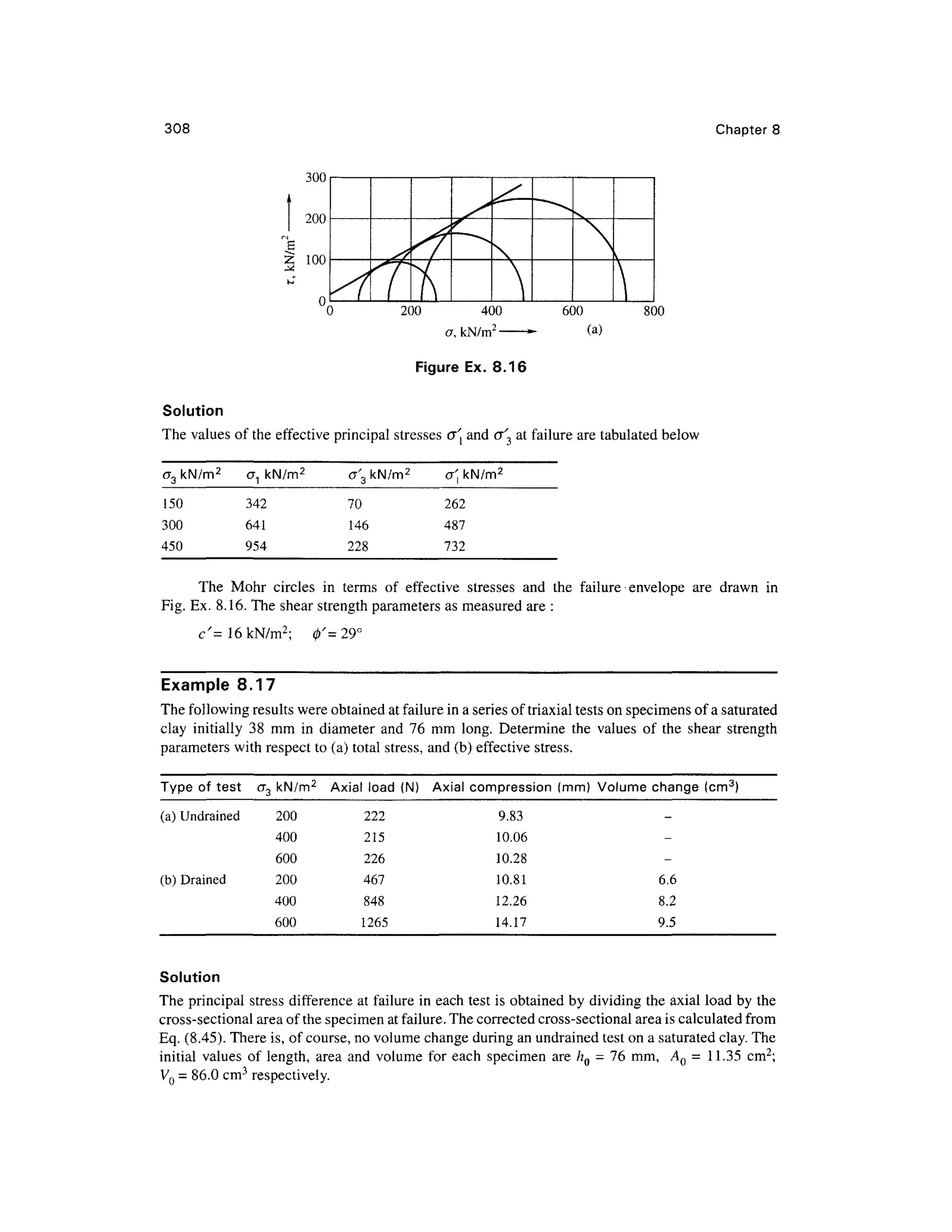
328. Shear Strengt h o f Soi l 309
'0 20 0 40 0 60 0 80 0 100 0 120 0
cr, kN/m2
-
Figure Ex. 8.17
The Mohr circles at failure and the corresponding failure envelopes for both series of tests are
shown in Fig. Ex. 8.17. In both cases the failure envelope is the line nearest to the common tangent
to the Mohr circles. The total stress parameters representing the undrained strength of the clay are:
cu = 85 kN/m2
; 0 u = 0
The effective stres s parameters, representin g the drained strength of the clay, are:
c' = 20 kN/m2
; 0 = 26°
a~ A/7//? n AWV n Are a (corrected ) a, - a- a,
3 0 0 1 3 1
a
b
kN/m2
200
400
600
200
400
600
0.129
0.132
0.135
0.142 0.07 7
0.161 0.09 5
0.186 0.11 0
cm2
13.04
13.09
13.12
12.22
12.25
12.40
kN/m2
170
160
172
382
691
1020
kN/m2
370
564
772
582
1091
1620
Example 8.1 8
An embankmen t is being constructed of soil whose properties ar e c'-107 1 lb/ft 2
, 0' = 21° (all
effective stresses) , an d y= 99.85 lb/ft3
. The pore pressure parameters as determined fro m triaxia l
tests are A = 0.5, and B = 0.9. Find the shear strength of the soil at the base of the embankment just
after th e heigh t o f fil l ha s bee n raise d fro m 1 0 ft t o 2 0 ft . Assume that the dissipatio n of por e
pressure during this stage of construction is negligible, and that the lateral pressure at any point is
one-half of the vertical pressure.
Solution
The equation for pore pressure is [Eq. (8.51)]
A« = 5JAcr3 +A(AcTj -Acr3)|
AcTj = Vertical pressure due to 1 0 ft of fill = 10 x 99.85 = 998.5 lb/ft2

329. 310 Chapter s
9985
ACT, = ^
^ = 499.25 lb/ft 2
3
2
Therefore, A w = 0.9[499.25 + 0.5 x 499.25] = 674 lb/ft 2
Original pressure, ^ = 10x99.85 = 998.5 lb/ft 2
Therefore, a' = <j} + A<JI - A w
= 998.5 + 998.5 -674 = 1323 lb/ft2
Shear strength, s = c' + a'tan0'= 1071 +1323tan21° = 1579 lb/ft 2
Example 8.1
9
At a depth o f 6 m below th e groun d surface a t a site , a van e shea r tes t gav e a torque valu e of
6040 N-cm. The vane was 10 cm high and 7 cm across the blades. Estimate the shear strength of the
soil.
Solution
Per Eq. (8.53)
Torque (r )
c =
where T = 6040 N-cm, L = 10 cm, r = 3.5 cm.
substituting,
6040 , „ X T , 7
c, =
= 6.4 N /cm2
- 6 4 kN/m2
" 2 x3.14 x 3.52
(10 +0.67 x 3.5) ~ °4 K1N/m
Example 8.20
A van e 11.2 5 c m long , an d 7. 5 c m i n diamete r wa s presse d int o sof t cla y a t th e botto m o f a
borehole. Torqu e was applied to cause failure of soil. The shear strength of clay was found t o be
37 kN/m2
. Determine the torque that was applied.
Solution
From Eq. (8.53) ,
Torque, T = cu [2nr2
(L + 0.67r)] wher e c u = 37 kN/m2
= 3.7 N/cm2
- 3.7 [2 x3.14 x (3.75)2
(11.25 + 0.67 x 3.75)] = 4500 N -cm
8.28 GENERA L COMMENT S
One o f the mos t importan t and the mos t controversial engineerin g propertie s o f soi l i s its shea r
strength. The behavior of soil under external load depends on many factors such as arrangement of
particles i n the soi l mass , it s mineralogical composition , wate r content, stres s histor y and many
others. The types of laboratory tests to be performed on a soil sample depends upon the type of soil

330. Shear Strengt h of Soi l 31 1
and its drainage condition during the application of external loads in the field. It is practically very
difficult (i f no t impossible ) t o obtai n undisturbe d samples o f granula r soil s fro m th e fiel d fo r
laboratory tests . I n suc h case s laborator y test s o n remolde d sample s ar e mostl y o f academi c
interest. Th e angl e o f shearin g resistanc e o f granula r soil s i s normall y determine d b y th e
relationships established betwee n<j) an d penetratio n resistance i n th e field . Th e accurac y o f this
method is sufficient fo r all practical purposes. The penetrometer used may be standard penetration
equipment or static cone penetrometer. Shear strength tests on cohesive soils depend mostly on the
accuracy with which undisturbed samples can be obtained from the field.
Undisturbed samples are extracted in sampling tubes of diameter 75 or 100 mm. Samples for
triaxial tests are extracted in the laboratory fro m the samples in the sampling tubes by using sample
extractors. Sample s ma y be disturbe d a t both the stage s o f extraction. If we are dealin g with a
highly overconsolidated clay the disturbance is greater at both the stages. Besides there is another
major disturbance which affects the test results very significantly. A highly overconsolidated clay is
at equilibrium in its in-situ conditions. The overconsolidation pressures of such soils could be of the
order 100 0 kPa (10 tsf) or more. The standard penetration value N in such deposits could be 100 or
more. The shear strength of such a soil under the in-situ condition could be in the order of 600 kPa
or more. But if an undisturbed sample of such a soil is tested in standard triaxial equipment, the
shear strength under undrained conditions could be very low. This is mostly due to the cracks that
develop on the surface of the samples du e to the relief o f the in-situ overburde n pressure on the
samples. Possibl y th e only way of obtaining the in-situ strength in the laboratory i s to bring back
the stat e o f th e sampl e t o it s origina l fiel d conditio n by applyin g all-aroun d pressure s o n th e
samples equal to the estimated overconsolidation pressures. This may not be possible in standard
triaxial equipment due to its limitations. The present practice is therefore to relate the in-situ shear
strength to some of the field tests such as standard penetration tests, static cone penetration tests or
pressuremeter tests.
8.29 QUESTION S AND PROBLEM S
8.1 Explai n Coulomb's equation for shear strength of a soil. Discuss the factors that affect th e
shear strength parameters of soil.
8.2 Explai n the method o f drawing a Mohr circle for a cylindrical sample i n a triaxial test.
Establish th e geometrica l relationship s betwee n th e stresse s o n th e failur e plan e an d
externally applied principal stresses.
8.3 Classif y th e shea r test s base d o n drainag e conditions . Explain ho w th e por e pressur e
variation and volume change take place during these tests. Enumerate the field conditions
which necessitate each of these tests.
8.4 Wha t are the advantages and disadvantages of a triaxial compression tes t in compariso n
with a direct shear test?
8.5 Fo r what types of soils, will the unconfmed compression test give reliable results? Draw a
Mohr circle for this test. How do you consider the change in the area of the specimen which
takes place during the test in the final results?
8.6 Wha t types o f field test s ar e necessary fo r determining the shear strengt h parameters of
sensitive clays? Derive the relationships that are useful fo r analyzing the observations of
this test.
8.7 Fo r loose and dense sands, draw the following typical diagrams:
(i) deviator stress vs. linear strain, and
(ii) volumetric strain vs. linear strain. Discuss them.
8.8 Discus s the effects of drainage conditions on the shear strength parameters of clay soil.
8.9 A direct shear test on specimens of fine sand gave the following results:

331. 312 Chapter s
Normal stress (lb/ft 2
) 210 0 370 0 450 0
Shearing stres s (lb/ft 2
) 97 0 170 0 208 0
Determine :
(i) the angle of internal friction o f the soil, and
(ii) shear strength of the soil at a depth of 1 5 ft from th e ground surface.
The specific gravity of solids is 2.65, void ratio 0.7 and the ground water table is at a depth
of 5 ft from the ground surface. Assume the soil above ground watar table is saturated.
A specime n o f clea n san d whe n subjecte d t o a direc t shea r tes t faile d a t a stres s o f
2520 lb/ft 2
when the normal stress was 3360 lb/ft2
.
Determine:
(i) the angle of internal friction, an d
(ii) the deviato r stres s a t which the failur e will take place, if a cylindrical sampl e o f the
same sand is subjected to a triaxial test with a cell pressure o f 2000 lb/ft2
. Fin d the angle
made by the failure plane with the horizontal.
A specimen o f fine sand, when subjected to a drained triaxial compression test , failed at a
deviator stress o f 8400 lb/ft2
. I t was observed tha t the failure plane made an angle of 30°
with the axis of the sample. Estimate the value of the cell pressure to which this specimen
would have been subjected.
8.12 A specimen of sandy silt, when subjected to a drained triaxial test failed at major and minor
principal stresses of 120 kN/m2
and 50 kN/m2
respectively. At what value of deviator stress
would another sample of the same soil fail,if i t were subjected to a confining pressur e of
75 kN/m2
?
8.13 A sand i s hydrostatically consolidated i n a triaxial test apparatus t o 8820 lb/ft2
an d then
sheared wit h the drainage valves open. At failure, (c^ - <7 3) is 22 kips/ft2
. Determin e the
major and minor principal stresses a t failure and the angle of shearing resistance .
8.14 Th e same sand as in Prob. 8.13 is tested in a direct shear apparatus under a normal pressure
of 8820 lb/ft2
. The sample fails when a shear stress of 5880 lb/ft2
is reached. Determin e the
major and minor principal stresses a t failure and the angle of shearing resistance. Plot the
Mohr diagram .
8.15 A sample of dense sand tested in a triaxial CD test failed along a well defined failure plane
at an angle of 66° with the horizontal. Find the effective confining pressure of the test if the
principal stres s difference at failure was 10 0 kPa.
8.16 A draine d triaxia l tes t i s performe d o n a san d wit h o^ , = 10. 5 kips/ft 2
. A t failur e
CTj'/cr^ = 4 . Find o^,, (<7j - <7 3)f and 0'.
8.17 I f the test of Prob. 8.1 6 had been conducte d undrained , determine (<J l - er 3)f, 0', 0tota[ and
the angle of the failure plane in the specimen. The pore water pressure u = 2100 lb/ft 2
.
8.18 I f the test of Prob. 8.16 is conducted at an initial confining pressure of 21 kips/ft2
, estimat e
the principal stress difference and the induced pore pressure at failure.
8.19 A sample of silty sand was tested consolidated drained in a triaxial cell where cr3 = 475 kPa.
If the total axial stress at failure was 160 0 kP a while<7 3 = 475 kPa , compute th e angle of
shearing resistance and the theoretical orientation of the failure plane with respect t o the
horizontal.
8.20 A drained triaxial test is to be performed on a uniform dense sand with rounded grains. The
confining pressure is 4200 lb/ft2
. At what vertical pressure wil l the sample fail?
8.21 Comput e the shearing resistance along a horizontal plane at a depth of 6.1 min a deposit of
sand. The water table is at a depth of 2.13 m. The unit weight of moist sand above the water

332. Shear Strengt h of Soi l 31 3
table is 18.54 kN/m3
and the saturated weight of submerged sand is 20.11 kN/m3
. Assume
that the sand is drained freely and(f) d fo r the wet sand is 32°.
A sampl e o f dr y san d wa s teste d i n a direc t shea r devic e unde r a vertica l pressur e of
137.9 kN/m2
. Comput e th e angl e o f interna l frictio n o f th e sand . Assum e shearin g
resistance = 96.56 kN/m2
.
The sand in a deep natural deposit has an angle of internal friction o f 40° in the dry state
and dry unit weight of 17.2 8 kN/m3
. If the water table is at a depth of 6.1 m, what is the
shearing resistance of the material along a horizontal plane at a depth of 3.05 m? Assume:
G^ = 2.68 .
8.24 Compute the shearing resistance under the conditions specified i n Prob. 8.23, if the water
table is at the ground surface.
8.25 A draine d triaxia l tes t wa s conducte d o n dens e san d wit h a confinin g pressur e o f
3000 lb/ft2
. The sample failed at an added vertical pressure of 11,000 lb/ft2
. Compute the
angle o f interna l frictio n 0 an d the angl e o f inclinatio n a o f th e failur e plane s o n the
assumption that Coulomb's law is valid.
A saturated sample of dense sand was consolidated in a triaxial test apparatus at a confining
pressure of 143. 6 kN/m 2
. Further drainage was prevented. During the addition of vertical
load, the pore pressure in the sample was measured. At the instant of failure, it amounted to
115 kN/m2
. The added vertical pressure at this time was 138.85 kN/m2
. What was the value
of 0 for the sand?
An undrained triaxial test was carried ou t on a sample of saturated clay with a confining
pressure o f 200 0 lb/ft2
. Th e unconfme d compressive strengt h obtaine d wa s 7300 lb/ft 2
.
Determine th e excess vertical pressure i n addition to the all-round pressure required t o
make the sample fail.
A series of undrained triaxial tests on samples of saturated soil gave the following results
cr3,kN/m2
10 0 20 0 30 0
u, kN/m2
2 0 7 0 13 6
(<TJ -cr3), kN/m2
29 0 40 0 53 4
Find the values of the parameters c and 0
(a) with respect to total stress, and (b) with respect to effective stress .
When an unconfmed compression test was conducted on a specimen of silty clay, it showed
a strength of 3150 lb/ft 2
. Determine the shear strength parameters of the soil if the angle
made by the failure plane with the axis of the specimen was 35°.
A normally consolidated cla y was consolidated unde r a stress o f 15 0 kPa, the n sheare d
undrained in axial compression. The principal stress difference at failure was 100 kPa and
the induced pore pressure at failure was 88 kPa. Determine analytically (a) the slopes of the
total and effective Mohr stress envelopes, and (b) the theoretical angle of the failure plane.
A normally consolidated clay sample wa s consolidated in a triaxial shea r apparatus at a
confining pressure of 21 kips/ft2
and then sheared under undrained condition. The (<Jl - <7 3)
at failure was 21 kips/ft2
. Determine 0 CM and a .
8.32 A CD axial compression triaxia l test on a normally consolidated cla y failed along a clearly
defined failure plane of 57°. The cell pressure during the test was 4200 lb/ft2
. Estimate 0',
the maximum o/
/o/
3, and the principal stress difference at failure.
Two identical sample s o f soft saturate d normall y consolidated cla y were consolidated t o
150 kPa in a triaxial apparatus. One specimen was sheared unde r drained conditions, and
the principa l stres s differenc e at failure was 30 0 kPa. The othe r specime n wa s sheare d
undrained, and the principal stress difference at failure was 200 kPa. Determine 0, and 0 .

333. 314 Chapter s
8.34 Whe n a triaxial compression tes t was conducted o n a soil specimen , i t failed a t an axial
pressure o f 7350 lb/ft 2
. I f the soil has a cohesion o f 105 0 lb/ft 2
an d a n angle of internal
friction o f 24° , wha t was th e cel l pressur e o f th e test ? Also fin d th e angl e mad e b y th e
failure plane with the direction of <7 3.
8.35 Give n the following triaxial test data, plot the results in a Mohr diagram an d determine 0 .
cr3 kN/m 2
Pea k <
69
138
207
7, kN/m 2
190
376
580
<T3 kN/m 2
276
345
414
Peak a , kN/m 2
759
959
1143
8.36 Tw o sets of triaxial tests were carrie d ou t on two samples of glacial silt . The results are
(a) <7 n = 400 kN/m 2
, <T 31 = 10 0 kN/m2
(b) cr 12 = 680 kN/m2
, cr32 = 200 kN/m2
.
The angl e o f th e failur e plan e i n bot h test s wa s measure d t o b e 59° . Determin e th e
magnitudes of 0 and c.
8.37 A triaxial compression tes t on a cylindrical cohesive sample gav e the following effective
stresses:
(a) Major principal stress, a/
l = 46,000 lb/ft 2
(b) Minor principal stress, tr'3 = 14,500 lb/ft2
(c) The angle of inclination of the rupture plane = 60° with the horizontal.
Determine analytically the (i) normal stress, (ii) the shear stress, (iii) the resultant stress on
the rupture plane through a point, and (iv) the angle of obliquity of the resultant stress with
the shear plane .
8.38 Give n the results of two sets of triaxial shear tests:
<7n = 180 0 kN/m 2
; cr 31 = 100 0 kN/m 2
<712 = 2800 kN/m2
; d32 = 2000 kN/m2
Compute 0 an d c.
8.39 Wha t is the shear strength in terms of effective stress on a plane within a saturated soil mass
at a point where the normal stress is 295 kN/m2
and the pore water pressure 12 0 kN/rn2
?
The effective stress parameters for the soil are c' = 12 kN/m2
, and 0' = 30° .
8.40 Th e effective stress parameters for a fully saturated clay are known to be c' = 315 lb/ft2
and
0' = 29° . I n a n unconsolidated-undraine d triaxial test o n a sample o f th e sam e cla y th e
confining pressur e wa s 525 0 lb/ft 2
an d th e principa l stres s differenc e a t failur e wa s
2841 lb/ft2
. What was the value of the pore water pressure in the sample a t failure?
8.41 I t is believed tha t the shear strength of a soil under certain conditions in the field will be
governed b y Coulomb's law, wherein c - 40 2 lb/ft2
, an d 0 = 22°. What minimum lateral
pressure woul d b e require d t o prevent failure of th e soi l a t a give n poin t i f the vertica l
pressure wer e 9000 lb/ft 2
?
8.42 Th e followin g data refe r t o thre e triaxia l tests performe d o n representativ e undisturbed
samples:
Test Cel l pressure kN/m 2
Axia l dial reading
(division) a t failure
1 5 0 6 6
2 15 0 10 6
3 25 0 14 7

334. Shear Strengt h of Soi l 31 5
The loa d dia l calibratio n facto r i s 1. 4 N per division . Eac h sampl e i s 7 5 mm lon g and
37.5 mm diameter. Fin d by graphical means, the value of the apparent cohesion an d the
angle of internal friction for this soil.
8.43 I n a triaxial test a soil specimen was consolidated under an allround pressure of 16 kips/ft2
and a back pressur e o f 8 kips/ft2
. Thereafter, unde r undrained conditions, th e allround
pressure was raised t o 1 9 kips/ft2
, resulting in a pore water pressure of 10. 4 kips/ft2
, then
(with th e confinin g pressure remainin g at 1 9 kips/ft2
) axia l loa d wa s applie d t o giv e a
principal stres s differenc e o f 12. 3 kips/ft 2
an d a por e wate r pressur e o f 13. 8 kips/ft 2
.
Calculate the values of the pore pressure coefficients A and B.
8.44 I n an in-situ van e test on a saturated cla y a torque of 35 N-m is required to shear the soil.
The vane is 50 mm in diameter and 10 0 mm long. What is the undrained strength of the
clay?
8.45 I n a vane test a torque of 46 N-m is required to cause failure of the vane in a clay soil. The
vane is 150 mm long and has a diameter of 60 mm. Calculate the apparent shear strength of
the soil from thi s test when a vane of 200 mm long and 90 mm in diameter i s used in the
same soil and the torque at failure was 138 N-m. Calculate the ratio of the shear strength of
the clay in a vertical direction to that in the horizontal direction .
8.46 A vane of 80 mm diameter and 160 mm height has been pushed into a soft clay stratum at
the bottom of a bone hole. The torque required to rotate the vane was 76 N-m. Determine
the undrained shear strength of the clay. After the test the vane was rotated severa l time s
and the ultimate torque was found to be 50 N-m. Estimate the sensitivity of the clay.
8.47 A normally consolidated deposi t of undisturbed clay extends to a depth of 1 5 m from the
ground surface with the ground water level at 5 m depth from groun d surface. Laboratory
test o n th e cla y give s a plasticit y inde x o f 68% , saturate d an d dr y uni t weight s o f
19.2kN/m3
an d 14. 5 kN/m3
respectively . A n undisturbe d specime n fo r unconfine d
compressive strengt h i s take n a t 1 0 m depth . Determin e th e unconfine d compressiv e
strength of the clay.
8.48 A triaxial sample was subjected to an ambient pressure of 200 kN/m2
, and the pore pressure
recorded wa s 5 0 kN/m 2
a t a full y saturate d state . Then th e cel l pressur e wa s raised t o
300 kN/m2
. What would be the value of pore pressure? At this stage a deviator stres s of
150 kN/m2
was applied to the sample. Determine the pore pressure assuming pore pressure
parameter A = 0.50.
In a triaxial test on a saturated clay, the sample was consolidated unde r a cell pressure of
160 kN/m2
. After consolidation, th e cel l pressur e wa s increased t o 35 0 kN/m2
, an d th e
sample was then failed under undrained condition. If the shear strength parameters of the
soil are c' = 15.2 kN/m2
, 0" = 26°, B = 1, and Af= 0.27, determine the effective majo r and
minor principal stresses at the time of failure of the sample .
A thi n layer of sil t exists a t a depth o f 1 8 m below th e surfac e of the ground . The sol i
above this level has an average dry unit weight of 15.1 kN/m3
and an average water content
of 36%. The water table is almost at the ground surface level. Tests on undisturbed samples
of the silt indicate the following values:
cu = 45 kN/m2
, 0u = 18°, c' = 36 kN/m2
and 0' = 27°.
Estimate the shearing resistance of the silt on a horizontal plane when (a) the shear stres s
builds up rapidly, and (b) the shear stress builds up slowly.

336. CHAPTER 9
SOIL EXPLORATION
9.1 INTRODUCTIO N
The stability of the foundation of a building, a bridge, an embankment or any other structure built
on soil depends on the strength and compressibility characteristic s o f the subsoil . The fiel d an d
laboratory investigations required to obtain the essential information on the subsoil is called Soil
Exploration or Soil Investigation. Soil exploration happens to be one of the most important parts of
Foundation Engineerin g an d a t th e sam e tim e th e mos t neglecte d par t o f it . Terzagh i i n 195 1
(Bjerrum, et al., 1960) had rightly remarked, that "Building foundations have always been treated
as step children". Hi s remark s ar e relevant even today. The succes s o r failur e o f a foundation
depends essentiall y o n th e reliabilit y o f th e variou s soi l parameter s obtaine d fro m th e fiel d
investigation an d laborator y testing , an d use d a s a n inpu t int o th e desig n o f foundations .
Sophisticated theories alone will not give a safe and sound design.
Soil exploration is a must in the present age for the design of foundations of any project. The
extent of the exploration depends upon the magnitude and importance of the project. Projects such
as buildings, power plants , fertilizer plants, bridges etc. , ar e localized i n areal extent. The are a
occupied b y suc h project s ma y var y fro m a fe w squar e meter s t o man y squar e kilometers .
Transmission lines, railway lines, roads and other such projects extend along a narrow path. The
length o f suc h project s ma y b e severa l kilometers . Eac h projec t ha s t o b e treate d a s pe r it s
requirements. Th e principl e o f soi l exploratio n remain s th e sam e fo r al l th e project s bu t th e
program and methodology may vary from project to project.
The element s o f soi l exploratio n depend mostl y on th e importanc e an d magnitud e of th e
project, but generally should provide the following:
1. Informatio n to determine the type of foundation required such as a shallow or deep foundation.
2. Necessar y informatio n with regards to the strength and compressibility characteristics of
the subsoil to allow the Design Consultant to make recommendations on the safe bearin g
pressure or pile load capacity.
317

337. 318 Chapter 9
Soil exploration involves broadly the following:
1. Plannin g of a program for soil exploration.
2. Collectio n o f disturbed and undisturbed soil or rock sample s fro m th e holes drilled i n the
field. The number and depths of holes depend upo n the project.
3. Conductin g al l the necessar y in-situ test s fo r obtaining the strengt h an d compressibilit y
characteristics of the soil or rock directly or indirectly.
4. Stud y of ground-water conditions and collection o f water samples fo r chemical analysis .
5. Geophysica l exploration , if required.
6. Conductin g all the necessary tests on the samples of soil /rock and water collected.
7. Preparatio n o f drawings, charts, etc.
8. Analysi s of the data collected .
9. Preparatio n o f report.
9.2 BORIN G O F HOLE S
Auger Metho d
Hand Operate d Augers
Auger boring i s the simplest of the methods. Han d operated or power drive n augers may be used .
Two types of hand operated auger s are in use as shown in Fig. 9.1
The depths of the holes are normally limited to a maximum of 10 mby this method. These augers
are generally suitable for all types of soil above the water table but suitable only in clayey soil below the
water table (excep t fo r the limitation s given below). A strin g of drill rods i s use d fo r advancing the
boring. Th e diameter s o f th e holes normall y var y fro m 1 0 to 2 0 cm. Han d operated auger s ar e not
suitable i n ver y stif f t o hard cla y no r i n granular soils below th e water table. Han d augerin g is not
practicable i n dense sand nor in sand mixed with gravel even if the strata lies above the water table.
Power Drive n Augers
In many countries the use of power drive n continuous flight augers i s the most popular method of
soil exploration for boring holes. The flights act as a screw conveyor to bring the soil to the surface.
Helical auger
Post hole auger
Extension
rod
Figure 9.1 Han d auger s

338. Soil Exploration 319
Sampler rod
Sampler
(a) (b)
Figure 9.2 Hollow-ste m auger
(a) Plugge d whil e advancin g th e auger , and (b ) plug removed an d sampler inserte d
to sampl e soil belo w auge r
This method may be used in all types of soil including sandy soils below the water table but is not
suitable if the soil is mixed with gravel, cobbles etc . The central ste m of the auger flight ma y be
hollow or solid. A hollow stem is sometimes preferred since standard penetration tests or sampling
may be done through the stem without lifting the auger from it s position in the hole. Besides, th e
flight o f auger s serve s th e purpos e o f casin g th e hole . Th e hollo w ste m ca n b e plugge d whil e
advancing th e bore an d th e plu g ca n be remove d whil e taking sample s o r conductin g standar d
penetration tests (to be described) a s shown in Fig. 9.2. The drilling rig can be mounted on a truck
or a tractor. Holes ma y be drilled by this method rapidly to depths of 60 m or more.
Wash Borin g
Wash boring is commonly used for boring holes. Soil exploration below the ground water table is
usually very difficult t o perform b y means of pits or auger-holes. Was h boring in such cases is a
very convenient method provided the soil is either sand, silt or clay. The method is not suitable if the
soil is mixed with gravel or boulders.
Figure 9.3 shows the assembly for a wash boring. To start with, the hole is advanced a short
depth by auger and then a casing pipe is pushed to prevent the sides from caving in. The hole is then
continued by the use of a chopping bit fixed at the end of a string of hollow drill rods. A stream of
water under pressure is forced through the rod and the bit into the hole, which loosens the soil as the
water flows up around the pipe. The loosened soi l in suspension in water is discharged int o a tub.
The soil in suspension settles down in the tub and the clean water flows into a sump which is reused
for circulation . The motiv e power for a wash boring is either mechanical o r man power. The bit
which is hollow is screwed to a string of hollow drill rods supported on a tripod by a rope or steel
cable passing over a pulley and operated b y a winch fixed on one of the legs of the tripod.

339. 320 Chapter 9
Swivel joint
Rope
Pulley
Tripod
Winch
Suction pipe
Chopping bit
Figure 9.3 Was h borin g
The purpose of wash boring is to drill holes only and not to make use of the disturbed washed
materials for analysis. Whenever an undisturbed sample is required at a particular depth, the boring
is stopped, and the chopping bit is replaced by a sampler. The sampler is pushed into the soil at the
bottom of the hole and the sample is withdrawn.
Rotary Drillin g
In the rotary drilling method a cutter bit or a core barrel with a coring bit attached to the end of a
string o f dril l rods i s rotated b y a power rig . Th e rotatio n of th e cuttin g bit shear s o r chips th e
material penetrated and the material is washed out of the hole by a stream of water just as in the case
of a was h boring . Rotary drillin g is use d primaril y for penetratin g the overburde n betwee n th e
levels of which samples are required. Coring bits, on the other hand, cut an annular hole around an
intact core which enters the barrel and is retrieved. Thus the core barrel is used primarily in rocky
strata to get rock samples .
As the rods with the attached bit or barrel are rotated, a downward pressure i s applied to the
drill string to obtain penetration, and drilling fluid under pressure is introduced int o the bottom of
the hole through the hollow drill rods and the passages in the bit or barrel. The drilling fluid serves
the dual function o f cooling the bit as it enters the hole and removing the cuttings from the bottom
of the hole as it returns to the surface in the annular space between the drill rods and the walls of the
hole. In an uncased hole, the drilling fluid also serves to support the walls of the hole. When boring

340. Soil Exploration 321
Water swive l
Tower mast
Swivel hol e
Stand pipe
Yoke and Kelly drive
Rotary driv e
Hoisting dr u Overflow ditc h
Bit, replaced by sampling spoo n
during sampling operation s
Figure 9.4 Rotar y drilling ri g (After Hvorslev , 1949 )
in soil, the drilling bit is removed and replaced by a sampler when sampling is required, but in rocky
strata the coring bit is used to obtain continuous rock samples. The rotary drilling rig of the type
given in Fig. 9.4 can also be used for wash boring and auger boring.
Coring Bit s
Three basic categories o f bits are in use. They are diamond, carbide insert, and saw tooth. Diamond
coring bits may be of the surface set or diamond impregnated type. Diamond coring bits are the
most versatile of all the coring bits since they produce high quality cores in rock materials ranging
from soft to extremely hard. Carbide insert bits use tungsten carbide in lieu of diamonds. Bits of this
type are used to core soft to medium hard rock. They are less expensive than diamond bits but the
rate of drilling is slower than with diamond bits. In saw-tooth bits, the cutting edge comprises a
series of teeth. The teeth are faced and tipped with a hard metal alloy such as tungsten carbide to
provide wear resistance and thereby increase th e life of the bit. These bit s are less expensive but
normally used to core overburden soil and very soft rocks only.
Percussion Drillin g
Percussion drilling is another method of drilling holes. Possibly this is the only method for drilling
in river deposits mixed with hard boulders of the quartzitic type. In this method a heavy drilling bit

341. 322 Chapter 9
is alternatively raised and dropped in such a manner that it powders the underlying materials which
form a slurry with water and are removed as the boring advances.
9.3 SAMPLIN G I N SOIL
Soils met in nature are heterogeneous in character with a mixture of sand, silt and clay in differen t
proportions. In water deposits, there are distinct layers of sand, silt and clay of varying thicknesses
and alternating with depth. We can bring all the deposits o f soil under two distinct groups for the
purpose of study, namely, coarse grained and fine grained soils. Soils with particles of size coarse r
than 0.075 mm ar e brought under the category o f coarse graine d an d those finer than 0.075 mm
under fine grained soils. Sandy soil falls in the group of coarse grained, and silt and clay soils in the
fine grained group. A satisfactory design of a foundation depends upon the accuracy with which the
various soil parameters require d fo r the design ar e obtained. The accuracy o f the soil parameter s
depends upo n the accuracy with which representative soil samples are obtained from the field.
Disturbed Sample s
Auger samples may be used to identify soil strata and for field classification tests, but are not useful
for laborator y tests . Th e cutting s or choppin g fro m was h boring s ar e o f littl e valu e excep t fo r
indicating change s i n stratificatio n to th e borin g supervisor . Th e materia l brough t u p wit h th e
drilling mud is contaminated and usually unsuitable even for identification.
For proper identificatio n and classification of a soil, representative sample s ar e required at
frequent interval s along the bore hole. Representative samples ca n usually be obtained by driving
or pushing into the strata in a bore hole an open-ended sampling spoon called a split spoon sample r
(Fig. 9.5) which is used for conducting standard penetration tests (refer Sect. 9.5). It is made up of
a driving shoe and a barrel. The barrel is split longitudinally into two halves with a coupling at the
upper end for connection to the drill rods. The dimensions of the split spoon are given in Fig. 9.5. In
a test the sampler i s driven into the soil a measured distance . After a sample i s taken, the cutting
shoe an d th e couplin g ar e unscrewe d an d the tw o halve s o f th e barrel separate d t o expos e th e
material. Experienc e indicate s tha t sample s recovere d b y thi s devic e ar e likel y t o b e highl y
disturbed and as such can only be used as disturbed samples. The samples so obtained are stored in
glass or plastic jars or bags, referenced an d sent to the laboratory for testing. If spoon samples ar e
to be transported to the laboratory without examination in the field, the barrel i s often cored out to
hold a cylindrical thin-walled tube known as a liner. After a sample has been obtained, the liner and
the sample it contains are removed from the spoon and the ends are sealed with caps or with metal
discs an d wax . Sample s o f cohesionles s soil s belo w th e wate r tabl e canno t b e retaine d i n
conventional sampling spoons without the addition of a spring core catcher.
3/4"
(19 mm)
3"
(76.2 mm ) 24" (60.96 cm)
8 Acme threads per inch
Water port 1/16 " dia
Make from 2 seamless
tubes to give full diamete r
(38.1 mm )
3/8"(34.93 mm)
Tool stee l drive shoe chisel
point tempered a t edge
3/4" dia steel ball
(19mm)
Thread for
wash pip e
or A rods
Figure 9.5 Spli t barre l sampler fo r standar d penetratio n tes t

342. Soil Exploratio n 323
Sampler head
Ball check valve
Rubber seat
Thin wall
sampling tube
Sampler
Many type s o f sampler s ar e i n us e fo r
extracting th e s o calle d undisturbe d samples .
Only two types of samplers are described here .
They are,
1. Ope n drive sampler,
2. Pisto n sampler.
Open Driv e Sample r
The wal l thickness o f th e ope n driv e sample r
used fo r samplin g ma y b e thi n o r thic k
according to the soil conditions met in the field.
The samplers are made of seamless steel pipes.
A thin-walled tube sampler is called a s shelby
tube sampler (Fig. 9.6), consist s of a thin wall
metal tub e connecte d t o a sample r head . The
sampler head contain s a ball chec k valv e and
ports whic h permit th e escap e o f wate r or air
from th e sampl e tub e as th e sampl e enter s it .
The thin wall tube, which is normally formed
from 1/1 6 to 1/ 8 inch metal, is drawn in at the
lower en d an d i s reame d s o tha t th e insid e
diameter o f th e cuttin g edg e i s 0. 5 t o 1. 5
percent les s than that of the inside diameter of the tube. The exact percentage i s governed by the
size and wall thickness of the tube. The wall thickness is governed by the area ratio, Ar, which is
defined a s
Figure 9.6 Thi n wall Shelby tub e
sampler
d2
-d2
Ar = ° ' x 100 percent , (9.1)
where, di - insid e diameter,
do - outsid e diameter .
Ar is a measure of the volume of the soil displacement to the volume of the collected sample . Well-
designed sampling tubes have an area ratio of about 10 percent. However, the area ratio may have to
be much more than 1 0 percent when samples are to be taken in very stiff to hard clay soils mixed
with stones to prevent the edges of the sampling tubes from distortion during sampling.
Sample Extraction
The thin-wall tub e sampler is primarily used for sampling i n soft t o medium stif f cohesiv e soils.
The wall thickness has to be increased if sampling is to be done in very stiff to hard strata. For best
results it is better to push the sampler statically into the strata. Samplers are driven into the strata
where pushing is not possible or practicable. The procedure of sampling involves attaching a string
of drill rods to the sampler tube adapter and lowering the sampler to rest on the bottom of the bore
hole which was cleaned of loose materials in advance. The sampler is then pushed or driven into the
soil. Over driving or pushing should be avoided. After the sampler is pushed to the required depth,
the soil at the bottom of the sampler is sheared off by giving a twist to the drill rod at the top. The
sampling tube is taken out of the bore hole and the tube is separated from the sampler head. The top
and bottom of the sample ar e either seale d wit h molten wax or capped to prevent evaporation of
moisture. The sampling tubes are suitably referenced for later identification.

343. 324 Chapter 9
Bore hole
Drill
Sampler head
Piston
Pressure cylinder
Casing pipe
A Hollo w
piston rod
Fixed pisto n
Sampler head
Air vent
Water under
pressure
Water return_
circulation
Hole in _
piston rod
_Thin- walled _
sampling tube
(a) (b) (c)
Figure 9.7 Osterber g Piston Sample r (a) Sampler i s set i n drilled hole , (b ) Sample tube
is pushed hydraulicall y int o the soil , (c ) Pressure is released through hole i n piston rod .
Piston Sample r (Afte r Osterber g 1952 )
To improve the quality of samples and to increase the recovery of soft o r slightly cohesive soils , a
piston sampler i s normally used. Such a sampler consists of a thin walled tube fitted with a piston
that closes the end of the sampling tube until the apparatus is lowered to the bottom of the bore hole
(Fig. 9.7(a)). Th e samplin g tub e i s pushe d int o th e soi l hydraulicall y b y keepin g th e pisto n
stationary (Fig. 9.7(b)). The presence o f the piston prevents the soft soil s fro m squeezing rapidly
into th e tub e an d thu s eliminates most o f th e distortion o f the sample . Th e pisto n als o help s t o
increase the length of sample that can be recovered b y creating a slight vacuum that tends to retain
the sample if the top of the column of soil begins to separate from the piston. During the withdrawal
of the sampler, the piston also prevents water pressure from acting on the top of the sample and thus
increases the chances of recovery. The design of piston samplers has been refined to the extent that
it is sometimes possible to take undisturbed samples of sand from below the water table. However,
piston sampling is relatively a costly procedure and may be adopted only where its use is justified.
Example 9. 1
The following dimensions are given for a shelby tube sampler:
External diameter = 51 mm
Internal diameter = 48 mm
Determine th e area ratio
Solution
Per Eq (9.1) the area ratio Ar is
A. =
482 = 0.129 = 12.9%

344. Soil Exploration 325
Example 9. 2
75 mm is the external diameter of a sampling tube. If the area ratio required is 20%, determine the
thickness of the sampling tube. In what type of clay would such a high area ratio be required?
Solution
152
-d2
Solving
The wall thickness
di = 68.465 mm.
75.0-68.465
= 3.267 mm
When sample s ar e to be taken in very stif f t o hard clay soils mixe d wit h stones, samplin g
tubes with high area ratios are required.
9.4 ROC K COR E SAMPLIN G
Rock coring is the process in which a sampler consisting of a tube (core barrel) with a cutting bit at
its lower end cuts an annular hole in a rock mass, thereby creating a cylinder or core of rock which
is recovered in the core barrel. Rock cores are normally obtained by rotary drilling.
The primary purpose of core drilling is to obtain intact samples. The behavior of a rock mass is
affected b y the presence o f fractures in the rock. The siz e and spacing of fractures, the degree o f
weathering of fractures, an d the presence of soil within the fractures ar e critical items . Figure 9.8
gives a schematic diagram of core barrels with coring bits at the bottom. As discussed earlier, the
cutting element may consist of diamonds, tungsten carbide inserts or chilled shot. The core barrel may
consist of a single tube or a double tube. Samples taken in a single tube barrel are likely to experience
Drill rod Drill rod
Fluid passage
Bearing
Outer barrel
Inner barrel
Core
lifter
a. Corin
g
^—bit
(a) (b)
Figure 9.8 Schemati c diagra m of cor e barrels (a) Single tube, (b ) Double tube.

345. 326 Chapter 9
considerable disturbanc e due to torsion, swellin g and contamination by the drilling fluid, bu t these
disadvantages ar e no t ther e i f th e coring i s conducte d i n hard, intact , rocky strata . However , i f a
double tub e barre l i s used, th e core i s protected fro m th e circulatin g fluid. Mos t cor e barrels ar e
capable of retaining cores up to a length of 2 m. Single barrel is used in Calyx drilling. Standard rock
cores range from about 11
A inches to nearly 6 inches in diameter. The more common sizes are given in
Table 9.1.
The recovery ratio R r, define d a s th e percentag e rati o betwee n th e lengt h o f th e cor e
recovered an d th e lengt h o f th e cor e drille d o n a give n run , i s relate d t o th e qualit y o f roc k
encountered i n boring, bu t it is also influenced by the drilling technique and the type and size of
core barrel used. Generally the use of a double tube barrel results in higher recovery ratio s than can
be obtaine d wit h singl e tub e barrels . A bette r estimat e o f in-sit u roc k qualit y i s obtaine d b y a
modified core recovery ratio known as the Rock Quality Designation (RQD) which is expressed a s
RQD = (9.2)
where, L a = total lengt h o f intac t har d an d soun d piece s o f cor e o f lengt h greate r tha n 4 in .
arranged i n its proper position,
Lt = total length of drilling.
Breaks obviously caused by drilling are ignored. The diameter of the core should preferably be not less
than 2V8 inches. Table 9.2 gives the rock quality description as related to RQD.
Table 9. 1 Standar d size s of cor e barrels , drill rods , an d compatible casin g
(Pecket al. , 1974 )
Core Barre l
Symbol
EWX, EW M
AWX, AWM
BWX, BW M
NWX, NW M
23
/4 x 37
/g
Hole
dia
(in)
l>/2
I15
/
1
'1 6
23
/8
3
37
/
j /g
Core
dia
(in)
1 6
1%
2'/8
2U
/16
Drill Ro d
Symbol
E
A
B
N
-
Outside
dia
(in)
115/16
1"V
I7
/
23
/
L
' 8
-
Casing
Symbol
_
EX
AX
BX
NX
Outside
dia
(in)
_
113/
16
2V4
2?
/8
3V2
Inside
dia
(in)
_
l'/2
I29
/
1
'3 2
23
/
z / 8
3
Note: Symbol X indicates single barrel, M indicates double barrel.
Table 9.2 Relatio n o f RQ D and in-situ Roc k Quality (Pec k et al., 1974 )
RQD % Rock Qualit y
90-100
75-90
50-75
25-50
0-25
Excellent
Good
Fair
Poor
Very Poor

346. Soil Exploratio n 32 7
9.5 STANDAR D PENETRATIO N TES T
The SP T is the mos t commonly used i n situ test in a bore hole in the USA . The tes t i s made by
making use of a split spoon sampler shown in Fig. 9.7. The method has been standardized as ASTM
D-1586 (1997) with periodic revision since 1958. The method of carrying out this test is as follows:
1. Th e spli t spoo n sample r i s connecte d t o a strin g o f dril l rod s an d i s lowere d int o th e
bottom of the bore hole which was drilled and cleaned in advance.
2. Th e sampler is driven into the soil strata to a maximum depth of 1 8 in by making use of a
140 Ib weight falling freely from a height of 30 in on to an anvil fixed on the top of drill rod.
The weight is guided to fall along a guide rod. The weight is raised and allowed to fall by
means of a manila rope, one end tied to the weight and the other end passing over a pulley
on to a hand operated winch or a motor driven cathead.
3. Th e number of blows required to penetrate each of the successive 6 in depths is counted to
produce a total penetration of 1 8 in.
4. T o avoid seating errors, the blows required for the first 6 in of penetration are not taken into
account; those required to increase the penetration from 6 in to 18 in constitute the N-value.
As per some codes of practice if the N-value exceeds 100 , it is termed as refusal, and the test
is stoppe d eve n i f th e tota l penetratio n fall s shor t o f th e las t 30 0 m m dept h o f penetration .
Standardization of refusal at 100 blows allows all the drilling organizations to standardize costs so
that highe r blow s i f require d ma y b e eliminate d t o preven t the excessiv e wea r an d tea r o f th e
equipment. The SPT is conducted normally at 2.5 to 5 ft intervals. The intervals may be increased
at greater depths if necessary.
Standardization o f SP T
The validit y of the SPT has been the subject of study and research b y man y authors for the last
many years . The basic conclusio n is that the best results are difficult t o reproduce. Som e o f the
important factors that affect reproducibilit y are
1. Variatio n in the height of fall of the drop weight (hammer) during the test
2. The number of turns of rope around the cathead, and the condition of the manila rope
3. Lengt h and diameter of drill rod
5. Diamete r of bore hole
6. Overburde n pressure
There ar e many more factor s that hamper reproducibility of results. Normall y correction s
used to be applied fo r a quick condition in the hole bottom due to rapid withdrawal of the auger.
ASTM 158 6 has stipulated standards to avoid such a quick condition. Discrepancies i n the input
driving energy an d its dissipation around the sampler int o the surrounding soil are the principal
factors for the wide range in N values. The theoretical input energy may be expressed as
Ein = Wh (9.3 )
where W = weight or mass of the hammer
h = height of fall
Investigation has revealed (Kovac s and Salomone, 1982 ) tha t the actual energy transferre d to the
driving head and then to the sampler ranged from about 30 to 80 percent. It has been suggested that
the SPT be standardized to some energy ratio Rg keeping in mind the data collected s o far from the
existing SPT. Bowles (1996) suggests that the observed SP T value N be reduced to a standard blow
count corresponding to 70 percent of standard energy. Terzaghi, et al., (1996) suggest 60 percent. The
standard energy ratio may be expressed as

347. 328 Chapte r 9
Actual hammer energy to sampler, Ea
ft, =
Input energy, Ein ^ '
Corrections to th e Observe d SP T Value
Three types o f corrections are normally applied t o the observed N values . They are :
1. Hamme r efficienc y correctio n
2. Drillrod , sampler an d borehole correction s
3. Correctio n du e to overburden pressure
1. Hamme r Efficienc y Correction, Eh
Different type s of hammers ar e i n use for drivin g the drill rods. Two types ar e normally used in
USA. They are (Bowles, 1996)
1. Donu t with two turns of manila rope on the cathead with a hammer efficiency Eh = 0.45.
2. Safet y with two turns of manila rope on the cathead with a hammer efficiency a s follows:
Rope-pulley or cathead = 0.7 to 0.8;
Trip or automatic hammer = 0.8 to 1.0 .
2. Dril l Rod , Sampler and Borehole Correction s
Correction factor s ar e use d fo r correctin g the effect s o f lengt h o f dril l rods , us e o f spli t spoo n
sampler with or without liner, and size of bore holes. The various correction factor s are (Bowles ,
1996).
a) Dril l rod length correction facto r C,
Length (m)
> 10m
4-10 m
<4.0m
Correction factor (Cd)
1.0
0.85-0.95
0.75
b) Sample r correction factor, Cs
Without liner Cx = 1.00
With liner,
Dense sand, clay = 0.80
Loose sand = 0.9 0
c) Bor e hole diameter correction factor, Cb
Bore hol e diameter Correctio n factor, C,
60-120 mm 1. 0
150mm 1.0 5
200mm 1.1 5
3. Correctio n Factor for Overburde n Pressure in Granular Soils, CN
The CN as per Liao and Whitman (1986) is

348. Soil Exploratio n 32 9
"95.761/2
.irj(9
-5)
where, p' 0 ^effective overburde n pressure in kN/m2
There ar e a number of empirical relations proposed fo r CN. However, the most commonly
used relationship is the one given by Eq. (9.5).
Ncor may be expressed as
"cor = C
NNE
h
C
d
C
sC
b (9-6 )
Ncor is related to the standard energy ratio used by the designer. Ncor may be expressed as A^70
or N^Q according to the designer's choice .
In Eq (9.6) CN N is the corrected valu e for overburden pressure only. The value of CN as per
Eq. (9.5) is applicable for granular soils only, whereas C^ = 1 for cohesive soils for all depths.
Example 9. 3
The observed standard penetration test value in a deposit of fully submerged sand was 45 at a depth
of 6.5 m. The average effective unit weight of the soil is 9.69 kN/m3
. The other data given are (a)
hammer efficienc y = 0.8, (b) drill rod length correction factor = 0.9, and (c ) borehole correction
factor = 1.05. Determine the corrected SPT value fo r standard energy (a) R - 6 0 percent, and (b)
Solution
Per Eq (9.6), the equation for N60 may be written as
(} N - C N F C C C
W ' V
60 ^N " ^h^d S ^b
where N
= observed SPT value
CN - overburde n correction
Per Eq (9.5) we have
1/2
= 95.7 6
N
Po
where p' Q
= effectiv e overburden pressure
= 6.5 x 9.69 = 63 kN/m2
Substituting fo r p' Q ,
CN= ^^
= 1.23 3
N
6 0
Substituting the known values, the corrected N60 is
N60 = 1.233 x 45 x 0.8 x 0.9 x 1.05 = 42
For 70 percent standar d energy
W70 =42x^ = 36
70
0. 7

349. 330 Chapte r 9
9.6 SP T VALUES RELATED TO RELATIV E DENSITY OF
COHESIONLESS SOILS
Although the SPT is not considered as a refined and completely reliabl e method of investigation,
the Ncor value s give usefu l informatio n with regard t o consistency of cohesive soil s an d relativ e
density of cohesionless soils . The correlation between N, r values and relative density of granular
soils suggested b y Peck, et al., (1974 ) is given in Table 9.3 .
Before usin g Table 9. 3 th e observe d N valu e has t o b e correcte d fo r standar d energ y an d
overburden pressure. The correlations given in Table 9.3 are just a guide and may vary according to
the fineness of the sand.
Meyerhof (1956) suggested the following approximate equations for computing the angle of
friction 0 from the known value of D f.
For granular soil with fine sand and more than 5 percent silt,
<p° = 25 + Q.15Dr (9.7 )
For granular soils with fine sand and less than 5 percent silt ,
0° = 30 + 0.15Dr (9.8 )
where Dr is expressed in percent.
9.7 SP T VALUES RELATE D TO CONSISTENC Y O F CLAY SOIL
Peck e t al. , (1974 ) hav e give n fo r saturate d cohesive soils , correlation s betwee n N cor valu e and
consistency. This correlation is quite useful bu t has to be used according to the soil conditions met
in the field. Table 9.4 gives the correlations.
The Ncor valu e to be used in Table 9.4 is the blow count corrected fo r standard energy ratio
Res. The present practice is to relate qu with Ncor as follows,
qu = kNcor kP a (9.9 )
Table 9.3 N an d 0 Related to Relativ e Densit y
N
cor
0-4
4-10
10-30
30-50
>50
Compactness
Very loos e
Loose
Medium
Dense
Very Dens e
Table 9. 4
Consistency
Very sof t
Soft
Medium
Stiff
Very Stif f
Hard
Relative density , D r (%)
Relation
"cor
0-2
2-4
4-8
8-15
15-30
>30
0-15
15-35
35-65
65-85
>85
Between Ncor an d qu
q , kP a
^ u'
<25
25-50
50-100
100-200
200-400
>400
0°
<28
28-30
30-36
36-41
>41
where qu is the unconfine d compressiv e strength .

350. Soil Exploratio n 33 1
or K =
7T- Kr a
(9.10 )
cor
where, k i s th e proportionalit y factor. A value of k = 12 has bee n recommende d b y Bowles
(1996).
Example 9. 4
For the corrected N values in Ex 9.3, determine the (a) relative density, and (b) the angle of friction.
Assume the percent of fines i n the deposit is less than 5%.
Solution
Per Table 9.3 the relative density and 0 are
For N60 = 42, Dr = 11%, 0 = 39°
For N70 = 36, Df= 71% , 0 =37.5°
Per Eq (9.8)
For D r = 77%, 0 = 30 + 0.15x77 = 41.5°
For D r = 71%, 0=30 + 0.15x71=40.7°
Example 9. 5
For the corrected values of N given in Ex 9.4, determine the unconfined compressive strength q u in
a clay deposit.
Solution
(a) Fro m Table 9.4
For N^ = 42
For N= 361 Q u
>
^00 kPa - The soil is of a hard consistency.
(b) Pe r Eq_(9.9;
qu= kN cor, wher e k = 1 2 (Bowles, 1996 )
For NM = 42, q = 12x42 = 504 kPa
Du • * M
For yV70 = 36, q u = 12 x 36 = 432 kPa
Example 9. 6
Refer t o Exampl e 9.3 . Determin e th e correcte d SP T valu e fo r R es = 10 0 percent , an d th e
corresponding values of Dr and 0. Assume the percent of fine sand in the deposit is less than 5%.
Solution
From Example 9.3, N60 = 42
„ °- 6
^
Hence Af, m = 2 x— ~ 25
1.0
From Table 9.3, 0 = 34.5° and Df = 57.5%
From Eq. (9.8) for Dr = 57.5%, 0 = 30 + 0.15 x 57.5 = 38.6°.

351. 332 Chapte r 9
9.8 STATI C CON E PENETRATION TEST (CRT )
The stati c con e penetratio n test normall y called th e Dutc h con e penetratio n tes t (CPT) . I t ha s
gained acceptanc e rapidl y in many countries. The metho d wa s introduce d nearl y 5 0 year s ago .
One of the greatest values of the CPT consists of its function a s a scale model pil e test. Empirical
correlations establishe d ove r many years permit the calculation of pile bearing capacit y directly
from th e CPT result s without the use of conventional soil parameters .
The CP T ha s proved valuabl e for soi l profiling a s the soil type can be identifie d from th e
combined measurement of end resistance of cone and side friction on a jacket. The test lends itself
to the derivatio n of norma l soil propertie s suc h as density, friction angl e an d cohesion . Variou s
theories hav e been developed for foundation design .
The popularity of the CPT can be attributed to the following three important factors:
1. Genera l introductio n of the electric penetromete r providin g more precis e measurements ,
and improvements in the equipment allowing deeper penetration.
2. Th e nee d fo r th e penetromete r testin g in-sit u techniqu e i n offshor e foundatio n
investigations in view of the difficultie s i n achieving adequate sampl e quality in marine
environment.
3. Th e additio n of other simultaneou s measurements t o the standar d frictio n penetromete r
such as pore pressure and soil temperature.
The Penetrometer
There ar e a variety of shapes and size s o f penetrometers bein g used. The on e that is standard in
most countries is the cone with an apex angle of 60° and a base area of 10 cm2
. The sleeve (jacket)
has becom e a standar d ite m o n th e penetromete r fo r mos t applications . O n th e 1 0 cm2
con e
penetrometer th e friction sleev e should have an area of 150 cm2
as per standard practice. The ratio
of sid e frictio n an d bearin g resistance , th e friction ratio, enables identificatio n of th e soi l typ e
(Schmertmann 1975 ) an d provide s usefu l informatio n in particular when n o bore hole dat a ar e
available. Even when borings are made, the friction rati o supplies a check on the accuracy of the
boring logs.
Two types of penetrometers are used which are based on the method used for measuring cone
resistance and friction. They are,
1. Th e Mechanical Type,
2. Th e Electrical Type.
Mechanical Type
The Begemann Friction Cone Mechanical type penetrometer is shown in Fig. 9.9. It consists of a 60°
cone with a base diameter of 35.6 mm (sectional area 10 cm2
). A sounding rod is screwed to the base.
Additional rods of one meter length each are used. These rods are screwed o r attached together to
bear agains t each other . The soundin g rods move inside mantle tubes. The inside diameter o f the
mantle tube is just sufficient fo r the sounding rods to move freel y wherea s th e outside diameter i s
equal to or less than the base diameter of the cone. All the dimensions in Fig. 9.9 are in mm.
Jacking System
The rigs used for pushing down the penetrometer consist basically of a hydraulic system. The thrust
capacity for cone testing on land varies from 20 to 30 kN for hand operated rigs and 100 to 200 kN
for mechanically operated rigs as shown in Fig. 9.10. Bourden gauges ar e provided in the driving
mechanism fo r measurin g th e pressure s exerte d b y th e con e an d th e frictio n jacke t eithe r
individually or collectively during the operation. The rigs may be operated eithe r on the ground or

352. Soil Exploratio n 333
mounted on heavy duty trucks. In either case, the rig should take the necessary upthrust. For ground
based rigs screw anchors are provided to take up the reaction thrust.
Operation o f Penetromete r
The sequence of operation of the penetrometer show n in Fig. 9.11 is explained a s follows:
Position 1 Th e cone and friction jacket assembly in a collapsed position.
Position 2 Th e cone is pushed down by the inner sounding rods to a depth a until a collar engages
the cone. The pressure gauge records the total force Qc to the cone. Normally a = 40 mm.
Position 3 Th e sounding rod is pushed further to a depth b. This pushes the friction jacket and the
cone assembly together; the force is Qt. Normally b = 40 mm.
Position 4 Th e outsid e mantl e tub e i s pushed dow n a distanc e a + b whic h bring s th e con e
assembly an d the friction jacket to position 1 . The total movement = a + b = 80 mm.
The process of operation illustrated above is continued until the proposed dept h is reached.
The cone is pushed at a standard rate of 20 mm per second. The mechanical penetrometer ha s its
advantage as it is simple to operate an d the cost o f maintenance is low. The qualit y of the work
depends on the skill of the operator. The depth of CPT is measured by recording the length of the
sounding rods that have been pushed into the ground.
35.7
266
35.6
i 3 0 3 5
Note: All dimensions are in mm.
Figure 9.9 Begeman n friction-cone mechanica l type penetromete r

353. 334 Chapter 9
iff
Hydraulically
operated cylinder
High pressure
manometer
Guide bow
Measuring
equipment
Road wheef
in raised position
Base fram e
3.5m
Upper support
beam
Guide column
Low pressure
manometer
LH maneuver ng handle
RH maneuvering handle
Control valv ;
Wooden sleepe r
1.80m-2.00m
PLAN
Fig. 9.10 Stati c con e penetratio n testing equipment
The Electri c Penetromete r
The electric penetromete r i s an improvement over the mechanical one. Mechanical penetrometer s
operate incrementally whereas the electric penetrometer i s advanced continuously.
Figure 9.12 shows an electric-static penetrometer wit h the friction sleeve just above the base
of the cone. The sectiona l are a o f the cone an d the surface area o f the friction jacket remai n the
same as those of a mechanical type. The penetrometer has built in load cells that record separatel y
the cone bearing an d side friction. Strai n gauges are mostly used for the load cells. The load cell s
have a norma l capacit y o f 5 0 t o 10 0 k N fo r en d bearin g an d 7. 5 t o 1 5 kN fo r sid e friction ,
depending o n the soils to be penetrated. An electric cabl e inserte d throug h the push rods (mantl e
tube) connect the penetrometer with the recording equipment at the surface which produces graph s
of resistance versu s depth.

354. Soil Exploration 335
Position 1
,
%
>1
A
'.a+ b
1
r.
a
I "
V
n
r
1
;/
V
1
1
^
!/
?
^
Sounding rod
Bottom mantle tube
Friction jacket
r M
Cone assembl y
Position 2
Position 3 Positio n 4
Figure 9.11 Fou r position s o f the soundin g apparatu s with friction jacket
The electri c penetromete r ha s many advantages. The repeatability o f the con e tes t i s very
good. A continuous record o f the penetration result s reflects better the natur e of the soi l layer s
penetrated. However, electronic cone testing requires skilled operators and better maintenance. The
electric penetrometer is indispensable for offshore soil investigation.
Operation of Penetrometer
The electri c penetromete r i s pushe d continuousl y at a standar d rat e o f 2 0 m m pe r second . A
continuous record of the bearing resistance qc and frictional resistance/^ against depth is produced
in the form of a graph at the surface in the recording unit.
Piezocone
A piezometer element included in the cone penetrometer is called apiezocone (Fig. 9.13). There is
now a growing use of the piezocone for measuring pore pressures at the tips of the cone. The porous
element is mounted normally midway along the cone tip allowing pore water to enter the tip. An
electric pressure transducer measures the pore pressure during the operation of the CPT. The pore
pressure record provides a much more sensitive means to detect thin soil layers. This could be very
important in determining consolidation rates in a clay within the sand seams.

355. Chapter 9
.
Piezocone.
1. Load cell
2. Friction sleeve
3. Water proof bushing
4. Cable
5. Strain gases
6. Connection with rods
7. Inclinometer
8. Porous stone (piezometer)
Figure 9.12 An-electric-stati c cone penetromete r
Temperature Cone
The temperatur e o f a soi l i s require d a t certai n localitie s t o provid e informatio n abou t
environmental changes. The temperature gradient with depth may offer possibilities to calculate the
heat conductivit y o f th e soil . Measuremen t o f th e temperatur e durin g CP T i s possibl e b y
incorporating a temperature sensor i n the electric penetrometer. Temperature measurement s hav e
been made in permafrost, under blast furnaces, beneath undercooled tanks, along marine pipe lines,
etc.
Effect o f Rat e of Penetration
Several studie s have been made to determine the effect o f the rate of penetration on cone bearin g
and side friction. Although the values tend to decrease for slower rates, th e general conclusio n is
that the influence is insignificant for speeds between 1 0 and 30 mm per second. The standard rate of
penetration has been generally accepted a s 20 mm per second.
Cone Resistanc ecr an d Loca l Side Frictio n f
cc »
Cone penetration resistance qc is obtained by dividing the total force Qc acting on the cone by the
base area A o f the cone.
(9.11)
Probe main frame
Pressure transducer
Retainer
Housing
Tip (Upper portion)
Porous element
Tip (lower portion)
Apex angle
Figure 9.1 3 Detail s of 60°/1 0 cm2
piezocon e

356. Soil Exploratio n 337
In the same way, the local side friction fc i s
Qf
fc=^^
A
f (9.12)
where, Q f = Qt - Q c = force required to push the friction jacket,
Qt = the total force required to push the cone and friction jacket together in the case of a
mechanical penetrometer ,
Af= surface area of the friction jacket.
Friction Ratio , Rf
Friction ratio, RAs expressed as
K fc
*/-—' (9.13 )
where fc an d qc are measured at the same depth. RAs expressed as a percentage. Friction ratio is an
important parameter for classifying soil (Fig. 9.16).
Relationship Betwee n qo, Relative Densit y Drand Friction Angle 0 for Sand
Research carried out by many indicates that a unique relationship between cone resistance, relative
density an d frictio n angl e valid for all sands doe s no t exist. Robertson an d Campanella (1983a )
have provided a set of curves (Fig. 9.14) which may be used to estimate Dr based on qc and effective
Cone bearing, qc MN/m2
0 1 0 2 0 3 0 4 0 5 0
•a 30 0
350
400
Dr expressed in percent
Figure 9.14 Relationshi p betwee n relativ e density D r and penetration resistanc e qc
for uncemente d quartz sands (Robertson and Campanella, 1983a )

357. 338 Chapter 9
Cone bearing, qc MN/m2
10 2 0 3 0 4 0
400
50
Figure 9.15 Relationshi p betwee n con e point resistance q c and angle of interna l
friction 0 for uncemente d quart z sand s (Robertso n and Campanella, 1 983b)
overburden pressure. These curves are supposed t o be applicable for normally consolidated clea n
sand. Fig. 9.15 gives the relationship between qc and 0 (Robertson and Campanella, 1983b) .
Relationship Betwee n qc and Undrained Shea r Strength , cu of Cla y
The cone penetration resistance qc and cu may be related as
or <lc - PC
(9.14)
where, Nk = cone factor,
po - y? = overburden pressure.
Lunne an d Kelve n (1981 ) investigate d the valu e o f th e con e facto r N k fo r bot h normall y
consolidated and overconsolidated clays. The values of A^ as obtained are given below:
Type o f cla y Cone factor
Normally consolidated
Overconsolidated
At shallow depths
At deep depths
11 to 1 9
15 to 2 0
12 to 1 8

358. Soil Exploratio n 339
10
Heavily
over consolidated
or cemented soil s
Sandy
gravel to
gravelly
sand to
sand
Sand to
silty sand
Silty sand
to sandy silt
Sandy silt to
clayey silt
Clayey silt to
silty clay
to clay /
Clay to
organic
clay
Highly
sensitive
soils
10'
1 2 3 4 5 6
Friction ratio (%)
Figure 9.16 A simplified classification chart (Douglas , 1984 )
Possibly a value of 20 for A^ for both types of clays may be satisfactory. Sanglerat (1972 )
recommends the same value for all cases where an overburden correction is of negligible value.
Soil Classificatio n
One of the basic uses of CPT is to identify and classify soils. A CPT-Soil Behavior Type Prediction
System ha s bee n develope d b y Dougla s an d Olse n (1981 ) usin g a n electric-frictio n con e
penetrometer. The classification is based on the friction ratio f/qc. Th e ratio f(/qc varie s greatly
depending on whether it applies to clays or sands. Their findings have been confirmed by hundreds
of tests.
For clay soils , i t has been foun d tha t the friction ratio decreases with increasing liquidity
index /, . Therefore , th e frictio n rati o i s a n indicato r o f th e soi l typ e penetrated . I t permit s
approximate identification of soil type though no samples are recovered .

359. 340 Chapter 9
f
1 Jc
0 5 0 10 0 15 0 20 0 25 0
/ an d qexpresse d in kg/cm
Friction ratio, Rf i n %
0
8
cfl
£ 1 6
<u
c
J3
8- 2 4
32
/in
1 2 3 4 5 Soi l profil e
r
C
r
i
v_
^
^- —•
"•' ^
„ '
^
-^-*
^
-—
c~
^
^ —
)
"X
^—•-
-
>
v
^
Sandy silt
Silts & silty clay
Silty sand
Silty clay
and
Clay
Sand
Silts & Clayey silts
Sands
Silty sand & Sandy silt
Figure 9.17 A typical sounding log
Douglas (1984) presented a simplified classification chart shown in Fig. 9.16. His chart uses
cone resistance normalize d (q ) for overburden pressure using the equation
q - q (l-1.251ogp' )
"en "c^ o * o'
where, p' = effective overburden pressure in tsf, and q = cone resistance in tsf,
(9.15)
In conclusion, CPT data provide a repeatable index of the aggregate behavior ofin-situ soil .
The CPT classification method provides a better picture of overall subsurface conditions than i s
available with most other methods o f exploration.
A typical sounding log is given in Fig. 9.17.

360. Soil Exploration 34 1
Table 9.5 Soi l classification base d on friction ratio R f (Sanglerat , 1972 )
Rf% Type of soi l
0-0.5
0.5-2.0
2-5
>5
Loose gravel fil l
Sands or gravels
Clay sand mixtures and silts
Clays, peats etc.
The friction ratio R, varies greatly with the type of soil. The variation of R, for the various
types of soils is generally of the order given in Table 9.5
Correlation Betwee n SP T an d CPT
Meyerhof (1965) presented comparative data between SPT and CPT. For fine or silty medium loose
to medium dense sands, he presents the correlation as
qc=OANMN/m2
His findings are as given in Table 9.6 .
(9.16)
Table 9.6 Approximat e relationshi p betwee n relativ e density o f fine sand, the SPT,
the static con e resistance and the angle of interna l fractio n (Meyerhof , 1965 )
State of san d D r N cof q c (MPa)</> °
Very loose <0. 2 < 4 <2. 0 <3 0
Loose 0.2-0. 4 4-1 0 2- 4 30-3 5
Medium dense 0.4-0. 6 10-3 0 4-1 2 35-4 0
Dense 0.6-0. 8 30-5 0 12-2 0 40-4 5
Very dense 0.8-1. 0 >5 0 >2 0 4 5
10
9
8
c 7
ll
16
^
o" 5
1 4
3
2
1
0
o.c
qc in kg/cm2
; N, blows/foo t
. A
^^
«*"^
k
^*
***^*
A
{*
A
A 4
**^n
A
k
A
A
/
/
A
A
)01 0.0 1 0. 1 1. 0
Mean grai n size D50, mm
Figure 9.18 Relationshi p betwee n qJN and mean grain size D50 (mm) (Robertson
and Campanella, 1983a )

361. 342 Chapte r 9
The lowes t value s o f th e angl e o f interna l frictio n give n i n Tabl e 9. 6 ar e conservativ e
estimates for uniform, clean sand and they should be reduced by at least 5° for clayey sand. These
values, as well as the upper values of the angles of internal friction which apply to well graded sand,
may be increased b y 5° for gravelly sand.
Figure 9.18 shows a correlation presented by Robertson an d Campanella (1983 ) between the
ratio of qJN an d mean grain size, D5Q. It can be seen from the figure that the ratio varies from 1 at
D5Q = 0.001 m m to a maximum value of 8 at D50 =1.0 mm. The soil type also varies from cla y to
sand.
It i s clear from the abov e discussion s tha t the valu e of n(= qJN) i s not a constant for any
particular soil. Designers must use their own judgment while selecting a value for n for a particular
type of soil.
Example 9. 7
If a deposit at a site happens to be a saturated overconsolidated cla y with a value of qc = 8.8 MN/m2
,
determine th e unconfmed compressiv e strength of clay given pQ = 127 kN/m2
Solution
Per Eq (9 . 14)
_
c., —
N " N
k k
Assume Nk = 20. Substituting the known values and simplifying
2(8800-127) _ _ , . . . ,
q
" =
-
2
0 -
=
If we neglect th e overburden pressure pQ
q ,
20
It i s clea r that , th e valu e of q u i s littl e affected b y neglectin g th e overburde n pressur e i n
Eq. (9.14 )
Example 9. 8
Static con e penetratio n test s wer e carrie d ou t a t a sit e b y usin g a n electric-frictio n con e
penetrometer. Th e following data were obtained at a depth of 12. 5 m.
cone resistance q c = 19.15 2 MN/m2
(200 tsf )
f
D _ J
C _ 1 -J
friction rati o A
/ ~ ~ l
-J
"c
Classify th e soil as per Fig. 9.16. Assume ^effective) = 16.5 kN/m3
.
Solution
The values of qc = 19.152 x 10 3
kN/m2
and Rf= 1.3 . Fro m Eq. (9.15)
q = 200 x 1-1.2 5 log 16
'5x12
'5
= 121 tsf
*cn & 1Q O
The soil is sand to silty sand (Fig. 9.16) fo r qm = 121 tsf and /?,= 1.3 .

362. Soil Exploration 34 3
Example 9. 9
Static cone penetration test at a site at depth of 30 ft revealed the following
Cone resistance q c = 12 5 tsf
Friction ratio R f= 1.3 %
The average effective uni t weight of the soil is 115 psf. Classify the soil per Fig. 9.16.
Solution
The effectiv e overburde n pressure p' 0 = 3 0 x 11 5 = 3450 lb/ft2
= 1.72 5 tsf
From Eq (9.15)
qm = 125 (1-1.25 log 1.725) = 88 tsf
Rf= 1.3%
From Fig. 9.16, the soil is classified as sand to silty sand for qcn = 88 tsf and Rf= 1.3%
Example 9.10
The stati c con e penetratio n resistance a t a sit e a t 1 0 m dept h i s 2.5 MN/m 2
. The frictio n rati o
obtained from the test is 4.25%. If the unit weight of the soil is 18.5 kN/m3
, what type of soil exists
at the site.
Solution
qc = 2.5 x 1000 kN/m2
= 2500 kN/m2
= 26.1 tsf
p'Q= 10 x 18. 5 = 185 kN/m2
=1.93 tsf
qcn = 26.1 (1-1.25 log 1.93) =16.8 tsf
Rf = 4.25 %
From Fig 9.16, the soil is classified as clayey silt to silty clay to clay
9.9 PRESSUREMETE R
A pressuremeter test is an in-situ stress-strai n test performed o n the walls of a bore hole using a
cylindrical prob e tha t ca n b e inflate d radially . The pressuremeter , whic h wa s firs t conceived ,
designed, constructed and used by Menard (1957) of France, has been in use since 1957 . The test
results are used either directly or indirectly for the design of foundations. The Menard test has been
adopted as ASTM Test Designation 4719. The instrument as conceived by Menard consists of three
independent chambers stacked one above the other (Fig. 9.19) with inflatable user membranes held
together at top and bottom by steel discs with a rigid hollow tube at the center. The top and bottom
chambers protec t th e middl e chambe r fro m th e en d effect s cause d b y th e finit e lengt h o f th e
apparatus, and these are known as guard cells. The middle chamber with the end cells together is
called the Probe. The pressuremeter consists of three parts, namely, the probe, the control unit and
the tubing.
The Pressuremete r Tes t
The pressuremeter test involves the following:
1. Drillin g of a hole
2. Lowerin g the probe into the hole and clamping it at the desired elevation
3. Conductin g the test

363. 344 Chapter 9
Volumeter
control unit
Pressure gaug e
Gas
Guard cell
Measuring cell
Guard cell
Guard cell
Measuring cel l
Water
Central tube
Guard cell
Gas
(a) (b)
Figure 9.1 9 Component s o f Menar d pressuremete r
Drilling an d Positionin g of Prob e
A Menar d pressur e tes t i s carrie d ou t i n a hol e drille d i n advance . The drillin g o f th e hol e i s
completed usin g a suitable drilling rig which disturbs the soil the least. The diameter of the bore
hole, Dh, in which the test is to be conducted shall satisfy th e condition
Dh < l.20Dp (9.17 )
where D i s the diameter of the probe under the deflated condition.
Typical sizes of the probe and bore hole are given in Table 9.7.
The probe i s lowered down the hole soon afte r borin g to the desired elevatio n and held in
position by a clamping device. Pressuremeter tests are usually carried out at 1 m intervals in all the
bore holes.
Conducting the Tes t
With the probe in position in the bore hole, the test is started by opening the valves in the control
unit for admitting water and gas (or water) to the measuring cell and the guard cells respectively .
The pressure i n the guard cells i s normally kept equal to the pressure in the measuring cell. The
pressures to the soil through the measuring cell are applied by any one of the following methods:
1 .Equa l pressure increment method,
2. Equa l volume increment method.

364. Soil Exploration 34 5
Table 9.7 Typica l sizes o f prob e an d bore hole fo r pressuremete r test
Hole dia.
designation
AX
BX
NX
Probe dia.
(mm)
44
58
70
/o
(cm)
36
21
25
/
(cm)
66
42
50
Bore hole dia.
Nominal
(mm)
46
60
72
Max.
(mm)
52
66
84
Note: /0 = length of measuring cell; / = length of probe.
If pressure is applied by the first method, each equal increment of pressure i s held constant
for a fixed length of time, usually one minute. Volume readings are made after one minute elapsed
time. Normally ten equal increments of pressure are applied for a soil to reach the limit pressure, pt.
If pressure is applied by the second method , the volume of the probe shall be increased i n
increments equal to 5 percent of the nominal volume of the probe (i n the deflated condition ) and
held constant for 30 seconds. Pressure readings are taken after 30 seconds of elapsed time .
Steps in both the methods are continued until the maximum probe volume to be used in the
test is reached. The test may continue at each position from 1 0 to 1 5 minutes. This means that the
test is essentially an undrained test in clay soils and a drained test in a freely drainin g material.
Typical Test Result
First a typical curve based on the observed readings in the field may be plotted. The plot is made of
the volume of the water read at the volumeter in the control unit, v, as abscissa fo r each increment
of pressure , /? , a s ordinate . Th e curv e i s a resul t o f th e tes t conducte d o n th e basi s o f equa l
increments of pressure and each pressure held constant for a period of one minute. This curve is a
raw curv e whic h requires som e corrections . Th e pressuremete r has , therefore , t o b e calibrate d
before it is used in design. A pressuremeter has to be calibrated for
1. Pressur e loss, pc,
2. Volum e loss vc,
3. Differenc e in hydrostatic pressure head H w.
Corrected Plo t o f Pressure-Volum e Curv e
A typical corrected plot of the pressure-volume curve is given in Fig. 9.20. The characteristic
parts of this curve are:
1. Th e initial part of the curve OA. This curve is a result of pushing the yielded wall of the hole
back t o the original position . At point A, th e at-rest conditio n is supposed t o have been
restored. The expansion of the cavity is considered onl y from point A. V Q is the volume of
water required to be injected over and above the volume Vc of the probe under the deflated
condition. If VQ is the total volume of the cavity at point A, we can write
V0=Vc + vQ (9.18 )
where vo is the abscissa of point A. The horizontal pressure at point A is represented asp owj.
2. Th e second par t of the curve is AB. This i s supposed to be a straight line portion o f the
curve and may represent the elastic range. Since AB gives an impression of an elastic range,
it is called the pseudo-elastic phase of the test. Point A is considered to be the start of the
pressuremeter test in most theories. Point B marks the end of the straight line portion of the
curve. The coordinates o f point B are pyand v« where py is known as the creep pressure.

365. 346 Chapte r 9
3. Curv e BC marks the final phase. The plastic phase is supposed to start from point fi, and the
curve become s asymptoti c a t poin t C a t a larg e deformatio n o f th e cavity . Th e limit
pressure, pr i s usually defined as the pressure that is required to double the initial volume
of the cavity. It occurs at a volume such that
v/-v0 =V0 =Vc + v0 (9.19 )
or v t= Vc + 2v0 (9.20 )
vQ i s normall y limite d t o abou t 30 0 cm 3
fo r probe s use d i n AX an d B X holes . Th e initia l
volume of these probes i s on the order o f 535 cm3
. This mean s that (V, + 2vQ) is on the order of
1135 cm3
. These values may vary according t o the design o f the pressuremeter .
The reservoi r capacit y i n the control uni t shoul d be of the order of 113 5 cm3
. In case the
reservoir capacity is limited and pl i s not reached within its limit, the test, has to be stopped at that
level. In such a case, the limit value, pr ha s to be extrapolated .
At-Rest Horizonta l Pressur e
The at-rest total horizontal pressure, poh, at any depth, z, under the in-situ condition before drilling
a hole may be expressed a s
Poh=(rz-u)KQ+u, (9.21 )
where u = pore pressure a t depth z,
7= gross unit weight of the soil,
KQ = coefficient of earth pressure for the at-rest condition.
The values of 7 and KQ are generally assumed taking into account the type and condition of
the soil. The pore pressure under the hydrostatic condition is
u = rw(z-hw), (9.22 )
where y w = unit weight of water,
hw = depth of water table from the ground surface.
As per Fig. 9.20 , pom i s the pressure whic h corresponds t o the volume V Q at the start of the
straight lin e portio n o f th e curve . Since i t has bee n foun d tha t i t i s ver y difficul t t o determin e
accurately pom, poh ma y not be equal to pom. As such, pom bear s no relation t o what the true earth
pressure at-res t is . I n Eq . (9.21 ) K Q ha s t o b e assume d an d it s accurac y i s doubtful . I n suc h
circumstances i t i s no t possibl e t o calculate poh. However , pom ca n b e use d fo r calculatin g th e
pressuremeter modulu s E . Th e experienc e o f man y investigator s i s tha t a self-borin g
pressuremeter give s reliable values for/?o/j.
The Pressuremete r Modulu s £m
Since the curve between points A and B in Fig. 9.20 is approximately a straight line, the soil in this
region ma y b e assume d t o behav e a s a mor e o r les s elasti c material . Th e equatio n fo r th e
pressuremeter modulu s may be expressed as
En =2G (l+u) = 2(1 + u)V — (9.23 )
p m
Av
where Gs is the shear modulus.
If V i s the volume at mid point (Fig 9.20), we may write,

366. 347
Injected volume
»~ Cavity volume
Figure 9.20 A typical corrected pressuremete r curv e
v
o+v
/
(9.24)
where Vc is the volume of the deflated portion of the measuring cell at zero volume reading on the
volumeter in the control unit.
Suitable values/or ^may be assumed in the above equation depending on the type of soil. For
saturated clay soils // is taken as equal to 0.5 and for freely draining soils, the value is less. Since Gs
(shear modulus) is not very much affected b y a small variation in ^u, Menard propose d a constant
value of 0.33 for /L As such the resulting deformation modulus is called Menard's Modulus Em. The
equation for Em reduces to
Em = 2.66Vm ^-(9.25 )
The followin g empirica l relationshi p ha s bee n establishe d fro m th e result s obtaine d fro m
pressuremeter tests . Undraine d shea r strengt h c u a s a functio n o f th e limi t pressur e~p l ma y b e
expressed as
c -
c
~ (9.26)
where p t = p
t- poh an d p oh = total horizontal earth pressure for the at rest condition.
Amar and Jezequel (1972) have suggested another equation of the form
Pi
c
«=
To+25kpa
where both p an d c ar e in kPa.
(9.27)

367. 348 Chapter 9
Example 9.1 1
A pressuremeter test was carried out at a site at a depth of 7 m below the ground surface. The water
table level was at a depth of 1. 5 m. The averag e unit weight of saturated soil is 17. 3 kN/m3
. Th e
corrected pressuremete r curve is given in Fig. Ex. 9.11 and the depleted volume of the probe is Vc
- 53 5 cm
3
. Determine the following.
(a) Th e coefficient o f earth pressure for the at-rest condition
(b) Th e Menard pressuremeter modulus Em
(c) Th e undrained shear strength cu. Assume that poh = pom i n this case
Solution
From Fig. Ex 9.11, p oh = pom = 105 kPa
The effective overburden pressur e is
P'Q = 17.3x7-5.5x9.81 =67.2 kPa
The effective horizonta l pressure is
p'0h= 105-5.5x9.81 = 51.0kPa
(a) From Eq (9.21)
51.0
u
P' 0 67. 2
(b) From Eq (9.25)
= 0.76
£*=2.66Vm
200 40 0 600 800 100 0
Volume cm
Figure Ex . 9.11

368. Soil Exploration 34 9
From Fig. Ex 9.11
vf = 200 cm3
p f = 530 kPa
v0 = 160 cm3
p om = 105 kPa
From Eq (9.24) V m = 5
35 +
= 715cm3
A 530-10 5
Av 200-16 0
Now Em = 2.66 x715 x 10.625 = 20,208 kPa
(c) From Eq (9.26)
9
From Fig Ex 9.11
845
Therefore c u = — = 94 kPa
From Eq (9.27)
c = ^ - + 25 =
— + 25 =109.5 kPa
" 1 0 1 0
9.10 TH E FLAT DILATOMETE R TES T
The/Zaf dilatometer i s a n in-situ testin g device develope d i n Italy by Marchetti (1980) . It is a
penetration devic e tha t include s a latera l expansio n arrangemen t afte r penetration . Th e test ,
therefore, combine s man y o f th e feature s containe d i n th e con e penetratio n tes t an d th e
pressuremeter test . This test has been extensively used for reliable, economical an d rapid in-situ
determination o f geotechnica l parameters . Th e fla t plat e dilatomete r (Fig . 9.21) consists o f a
stainless steel blade with a flat circular expandable membrane of 60 mm diameter on one side of the
stainless steel plate, a short distance above the sharpened tip. The size of the plate is 220 mm long,
95 mm wide and 14 mm thick. When at rest the external surface of the circular membrane is flush
with the surrounding flat surface of the blade.
The prob e i s pushed t o the required dept h by making use o f a rig use d fo r a static con e
penetrometer (Fig. 9.10). The probe is connected to a control box at ground level through a string of
drill rods, electric wires for power supply and nylon tubing for the supply of nitrogen gas. Beneath
the membrane is a measuring device which turns a buzzer off in the control box. The method of
conducting the DMT is as follows:
1. Th e probe is positioned at the required level. Nitrogen gas is pumped into the probe. When
the membrane is just flush with the side of the surface, a pressure reading is taken which is
called the lift-off pressure . Approximate zero corrections are made. This pressure is called
Pi-
2. Th e probe pressure is increased until the membrane expands by an amount A/ = 1. 1 mm.
The corrected pressure is pr

369. 350 Chapter 9
3. Th e next step is to decrease th e pressure until the membrane returns to the lift off position.
This correcte d readin g i s py Thi s pressur e i s relate d t o exces s por e wate r pressur e
(Schmertmann, 1986) .
The details of the calculation lead to the following equations.
p,
,
1 .Materia l index , I = —
p2-u
2. Th e latera l stres s index , K n = Pi -u
3. Th e dilatomete r modulus , E D = 34.7 (p2 - p {) kN/m 2
(9.28)
(9.29)
(9.30)
where, p' = effective overburden pressure = y'z
u = pore water pressure equal to static water level pressure
Y - effectiv e unit weight of soil
z = depth of probe leve l from ground surface
The latera l stres s inde x KD i s related t o KQ (th e coefficient of earth pressure fo r th e at-res t
condition) and to OCR (overconsolidation ratio).
Marchetti (1980) has correlated severa l soil properties as follows
K,
0.47
1.5
0.6
(9.31)
(9.32)
Wire
Pneumatic
tubing
14 m m
membrane
--
[
L
c
J
4-Pi
Flexible
membrane
-Vn
—
/
1.1 m m
Figure 9.21 Illustratio n o f a flat plat e dilatomete r (afte r Marchetti 1980 )

370. Soil Exploratio n 351
200
05
o.. 0.2 0. 3 0.60. 8 1. 2 1. 8 3. 3
Material index ID
Figure 9.22 Soi l profile based on dilatometer test (afte r Schmertmann, 1986 )
= (0.5K D)1.6
(9.33)
(9.34)
where Es is the modulus of elasticity
The soil classification as developed by Schmertmann (1986) is given in Fig. 9.22. /D is related
with ED in the development of the profile.
9.11 FIEL D VANE SHEA R TEST (VST)
The vane shear test is one of the in-situ tests used for obtaining the undrained shear strength of soft
sensitive clays. It is in deep beds of such material that the vane test is most valuable for the simple
reason that there is at present no other method known by which the shear strength of these clays can
be measured. The details of the VST have already been explained in Chapter 8.
9.12 FIEL D PLATE LOAD TEST (PLT)
The fiel d plat e tes t i s th e oldes t o f th e method s fo r determinin g either th e bearin g capacit y o r
settlement of footings. The details of PLT are discussed under Shallow Foundations in Chapter 13 .

371. 352 Chapter 9
9.13 GEOPHYSICA L EXPLORATIO N
The stratificatio n of soil s an d rock s ca n b e determine d b y geophysica l method s o f exploratio n
which measur e change s i n certai n physica l characteristic s o f thes e materials , fo r exampl e th e
magnetism, density, electrical resistivity, elasticity or a combination of these properties. However ,
the utility of these methods in the field of foundation engineering is very limited since the methods
do no t quantif y th e characteristic s o f th e variou s substrata . Vita l informatio n o n groun d wate r
conditions i s usuall y lacking . Geophysica l method s a t bes t provid e som e missin g informatio n
between widely spaced bore holes but they can not replace bore holes. Two methods of exploration
which are some times useful ar e discussed briefly in this section. They ar e
D, D , D , D A D
Velocity V }
Velocity V 2
Rocky strat a
Velocity V3
(a) Schematic representation of refraction method
Layer 1
Layer 2
R
R,
Electrode spacing Electrod e spacin g
(b) Schematic representation of electrical resistivity metho d
Figure 9.23 Geophysica l methods of exploratio n

372. Soil Exploratio n 35 3
1. Seismi c Refractio n Method,
2. Electrica l Resistivity Method.
Seismic Refractio n Metho d
The seismi c refractio n metho d i s based o n the fact tha t seismic wave s have different velocitie s in
different types of soils (or rock). The waves refract when they cross boundaries between different types
of soils. If artificial impulses are produced either by detonation of explosives or mechanical blows with
a heavy hammer at the ground surface or at shallow depth within a hole, these shocks generate thre e
types of waves. In general, only compression waves (longitudinal waves) are observed. These waves are
classified as either direct, reflected or refracted. Direct waves travel in approximately straight lines from
the source of the impuls e to the surface. Reflected or refracted waves undergo a change in direction
when they encounter a boundary separating media of different seismic velocities. The seismic refraction
method is more suited to shallow exploration for civil engineering purposes.
The method start s by inducing impact or shock wave s into the soil a t a particular location.
The shoc k wave s ar e picked u p by geophones . I n Fig. 9.23(a), point A i s the sourc e o f seismi c
impulse. The points D^ throug h Dg represent the locations of the geophones or detectors which are
installed in a straight line. The spacings o f the geophones ar e dependent o n the amount of detail
required and the depth of the strata being investigated. In general, the spacing must be such that the
distance fro m D j t o D8 is three t o fou r time s th e dept h t o be investigated . Th e geophone s ar e
connected by cable to a central recording device. A series of detonations or impacts are produced
and th e arriva l tim e o f th e firs t wav e a t each geophon e positio n i s recorded i n turn . When th e
distance between source and geophone is short, the arrival time will be that of a direct wave. When
the distance exceeds a certain value (depending on the thickness of the stratum), the refracted wave
will be the first to be detected by the geophone. This is because the refracted wave, although longer
than that of the direct wave, passes through a stratum of higher seismic velocity.
A typical plot of test results for a three layer system is given in Fig. 9.23(a) with the arrival
time plotted agains t th e distance sourc e an d geophone. A s in the figure, if the source-geophon e
spacing is more tha n the distance dr whic h is the distance from th e source to point B, the direct
wave reaches the geophone i n advance of the refracted wave and the time-distance relationshi p is
represented b y a straight lin e AB throug h the origin represented b y A. I f on the other hand , the
source geophon e distanc e i s greater tha n d{ , the refracted wave s arriv e i n advance o f the direc t
waves and the time-distance relationship is represented by another straight line BC which will have
a slope different fro m tha t of AB. The slopes of the lines AB and BC are represented b y IVr an d
1/V2 respectively, wher e V { an d V 2 are th e velocitie s of the uppe r an d lowe r strat a respectively .
Similarly, the slope of the third line CD is represented b y 1/V 3 in the third strata.
The general type s of soil or rocks can be determined fro m a knowledge of these velocities .
The depth H{ o f the top strata (provided the thickness of the stratum is constant) can be estimated
from the formula
(9.35a)
2 ' " 1
The thickness of the second layer (//2) is obtained fro m
The procedure is continued if there are more than three layers.
If the thickness of any stratum is not constant, average thickness is taken.

373. 354 Chapter 9
Table 9.8 Rang e of seismi c velocitie s i n soils nea r the surfac e or at shallo w
depths (afte r Peck et al., 1974 )
Material
1. Dry silt , sand, loose gravel, loam, loose rock talus, and
moist fine-graine d to p soil
2. Compact till, indurated clays, compact clayey gravel,
cemented san d and sand clay
3. Rock, weathered, fractured or partly decomposed
4. Shale, sound
5. Sandstone, sound
6. Limestone, chalk, sound
7. Igneous rock, soun d
8. Metamorphic rock , soun d
Velocity
ft/sec m/se c
600-2500
2500-7500
2000-10,000
2500-11,000
5000-14,000
6000-20,000
12,000-20,000
10,000-16,000
180-760
760-2300
600-3000
760-3350
1500-4300
1800-6000
3650-6000
3000-4900
The following equations may be used for determining the depths H, an d H2 i n a three layer
strata:
t,V,
2 cos a
(9.36)
2 cos/?
(9.37)
where t { = AB r (Fig . 9.23a); th e poin t Bl i s obtaine d o n th e vertica l passin g throug h A b y
extending the straight line CB,
t2 = (AC j - A5j); ACj is the intercept on the vertical through A obtained by extending the
straight line DC,
a = sin~ l
(V/V 2),
j8 = sin- 1
(V2/V3). (9.38 )
a and (3 are the angles of refraction of the first and second stratum interfaces respectively .
The formulae used to estimate the depths from seismic refraction survey data are based on the
following assumptions:
1. Eac h stratum is homogeneous and isotropic .
2. Th e boundaries between strata are either horizontal or inclined planes.
3. Eac h stratum is of sufficient thickness to reflect a change in velocity on a time-distance plot.
4. Th e velocity of wave propagation for each succeeding stratum increases with depth.
Table 9. 8 give s typica l seismi c velocitie s i n variou s materials . Detaile d investigatio n
procedures fo r refraction studies are presented by Jakosky (1950).
Electrical Resistivit y Metho d
The method depends on differences in the electrical resistance of different soi l (and rock) types. The
flow o f curren t through a soi l i s mainl y due t o electrolyti c action an d therefor e depend s o n th e

374. Soil Exploration 35 5
concentration o f dissolved salt s i n the pores. Th e minera l particle s o f soil ar e poor conductor s o f
current. The resistivity of soil, therefore, decreases as both water content and concentration of salts
increase. A dense clean sand above the water table, for example, would exhibit a high resistivity due
to its low degree o f saturation and virtual absence o f dissolved salts. A saturated clay of high void
ratio, on the other hand, would exhibit a low resistivity due to the relative abundance of pore water and
the free ions in that water.
There are several methods by which the field resistivity measurements are made. The most
popular of the methods is the Wenner Method.
Wenner Metho d
The Wenner arrangement consist s o f four equally spaced electrodes driven approximately 20 cm
into the ground as shown in Fig. 9.23(b). In this method a dc current of known magnitude is passed
between th e tw o oute r (current ) electrodes , thereb y producin g withi n th e soi l a n electri c field ,
whose patter n i s determine d b y th e resistivitie s o f th e soil s presen t withi n th e fiel d an d th e
boundary conditions. The potential drop E for the surface current flow lines is measured by means
of the inner electrodes. Th e apparent resistivity, R, is given by the equation
R = — —(9.39 )
It is customary to express A in centimeters, E in volts, / i n amperes, an d R ohm-cm. The apparent
resistivity represents a weighted average of true resistivity to a depth A in a large volume of soil, the
soil close to the surface being more heavily weighted than the soil at greater depths. The presence of
a stratum of low resistivity forces the current to flow closer to the surface resulting in a higher voltage
drop and hence a higher value of apparent resistivity. The opposite is true if a stratum of low resistivity
lies below a stratum of high resistivity.
The metho d know n a s sounding i s use d whe n th e variatio n o f resistivit y wit h dept h i s
required. This enable s rough estimates t o be made o f the types and depths o f strata. A series of
readings ar e taken , th e (equal ) spacin g o f th e electrode s bein g increase d fo r eac h successiv e
reading. However , th e cente r o f th e fou r electrode s remain s a t a fixed point . As th e spacin g i s
increased, the apparent resistivity is influenced by a greater depth of soil. If the resistivity increases
with the increasing electrod e spacings , i t can be concluded tha t an underlying stratum of higher
resistivity i s beginnin g t o influenc e th e readings . I f increase d separatio n produce s decreasin g
resistivity, on the other hand, a lower resistivity is beginning to influence the readings.
Apparent resistivity is plotted against spacing, preferably, on log paper. Characteristic curves
for a two layer structure are shown in Fig. 9.23(b). For curve Cp the resistivity of layer 1 is lower
than that of 2; for curve C2, layer 1 has a higher resistivity than that of layer 2. The curves become
asymptotic to lines representing the true resistance Rr and R2 of the respective layers. Approximate
layer thickness can be obtained b y comparing the observed curve s of resistivity versus electrod e
spacing with a set of standard curves.
The procedure known as profilingi s used in the investigation of lateral variation of soil types.
A series of readings is taken, the four electrodes being moved laterally as a unit for each successiv e
reading; the electrode spacing remains constant for each reading of the series. Apparent resistivity
is plotted against the center position of the four electrodes, t o natural scale; such a plot can be used
to locate the position of a soil of high or low resistivity. Contours of resistivity can be plotted over
a given area.
The electrica l metho d o f exploratio n ha s bee n foun d t o be no t a s reliable a s the seismi c
method as the apparent resistivity of a particular soil or rock can vary over a wide range of values.
Representative values of resistivity are given in Table 9.9 .

375. 356 Chapter 9
Table 9. 9 Representativ e value s o f resistivity . The values ar e expressed i n units of
103
ohm-cm (afte r Pec k et al., 1974 )
Material Resistivity ohm-c m
Clay and saturated silt
Sandy clay and wet silty san d
Clayey sand and saturated sand
Sand
Gravel
Weathered roc k
Sound roc k
0-10
10-25
25-50
50-150
150-500
100-200
150-4,000
Example 9.12
A seismic survey was carried out for a large project t o determine th e nature of the substrata. Th e
results of the survey are given in Fig. Ex 9.12 in the form of a graph. Determine th e depths of the
strata.
Solution
Two methods may be used
1. Us e of Eq (9.35)
2. Us e of Eqs (9.36) an d (9.37 )
First we have to determine th e velocities i n each stratu m (Fig. Ex. 9.12) .
I
V, ."/••/.':.'•>•'••" - Surface soil•.•'. ";:.i.'.-"::)
: H
V2 •. • ''.';: . Sand and loose gravel
Rock
Afl, = 8.75 x 10'3
sec
AC, = 33.75 x 10'3
sec
AC2 = 38.75 x 10~ 3
sec
J,=2.188m
d2 = 22.5 m
A5=12.75x 10'3
sec
H,
20 d ^ 3 0
Distance m
40 50
Figure Ex. 9.12

376. Soil Exploratio n 35 7
distance 2.18 8
= — -
AB 12.75X1CT 3
= 172 m /sec
V = -
2 -
= -
-
_= 750 m/sec
7
2
AC-ABl (7.75 - 1.75)5
In the same way, the velocity in the third stata can be determined. The velocity obtained is
V3 = 2250 m/sec
Method 1
From Eq (9.35 a), the thickness H{ o f the top layer is
2.188 /750-17 2
= 0.83 m
2 V 100 0
From Eq (9.35b) the thickness H2 is
i/ no < no a 22
'5
2250-75 0
H>> =0.85x0.83 +—
3000
= 0.71 +7.955 = 8.67m
Method 2
From Eq (9.36)
1
2 cos a
t{ = ABl = 1.75 x 5 x1Q-3
sec(Fig.Ex.9.12)
i V ,i 17 2
a = sin !
—L
=sin l
= 13.26°
V2 75 0
cosa = 0.9733
__ 12.75xlQ- 3
xl72
//, =
= 1.13 m
1
2x0.973 7
From Eq (9.37)
t2V2
2
2cos/ 7
t2 = 5x 5 x10~3
sec
, 75 0
/?= shr1
—— = 19.47°; cos J3=0.9428
2250
_5x5xlO"3
x750
2
~ 2x0.942 8
n f t .
= 9.94m

377. 358 Chapte r 9
9.14 PLANNIN G O F SOIL EXPLORATION
The planner has to consider the following points before makin g a program:
1. Type , size and importance of the project.
2. Whethe r the site investigation is preliminary or detailed.
In the case of large projects, a preliminary investigation is normally required for the purpose of
1. Selectin g a site and making a feasibility study of the project,
2. Makin g tentative designs and estimates of the cost of the project.
Preliminary site investigation needs only a few bore holes distributed suitably over the area for
taking samples. The data obtained from the field and laboratory tests must be adequate to provide a fairly
good idea of the strength characteristics of the subsoil for making preliminary drawings and design. In
case a particular site is found unsuitable on the basis of the study, an alternate site may have to be chosen.
Once a sit e i s chosen , a detaile d soi l investigatio n is undertaken . The plannin g of a soi l
investigation includes the following steps:
1. A detailed study of the geographical condition of the area which include
(a) Collectio n of all the available information about the site, including the collection of
existing topographical and geological maps ,
(b) Genera l topographical features of the site,
(c) Collectio n o f th e availabl e hydrauli c conditions, suc h a s wate r tabl e fluctuations ,
flooding of the site etc,
(d) Acces s to the site.
2. Preparatio n o f a layout plan of the project.
3. Preparatio n o f a borehole layou t plan which includes the depths an d the number of bore
holes suitabl y distributed over the area.
4. Markin g on the layout plan any additional types of soil investigation.
5. Preparatio n of specifications and guidelines for the field execution of the various elements
of soil investigation.
6. Preparatio n o f specification s an d guid e line s fo r laborator y testin g o f th e sample s
collected, presentatio n of field and laboratory test results, writing of report, etc .
The planner can make an intelligent, practical and pragmatic plan if he is conversant with the
various elements of soil investigation.
Depths an d Numbe r o f Bor e Hole s
Depths o f Bor e Holes
The depth up to which bore holes should be driven is governed by the depth of soil affected by the
foundation bearin g pressures . The standard practice i s to take th e borings t o a depth (calle d th e
significant depth) at which the excess vertica l stress caused by a fully loade d foundatio n is of the
order of 20 per cent or less of the net imposed vertical stress at the foundation base level. The depth
the borehole as per this practice works out to about 1.5 times the least width of the foundation from
the base leve l of the foundation as shown in Fig. 9.24(a). Where stri p or pad footings are closely
spaced whic h results in the overlapping of the stressed zones , th e whole loaded are a become s i n
effect a raft foundation with correspondingly deep borings as shown in Fig. 9.24(b) and (c). In the
case of pile or pier foundations the subsoil should be explored t o the depths required to cover the
soil lyin g even below the tips of piles (o r pile groups) and piers whic h are affecte d b y the load s
transmitted t o th e deepe r layers , Fig . 9.24(d). I n cas e roc k i s encountere d a t shallo w depths ,
foundations ma y hav e t o res t o n rock y strata . Th e borin g shoul d als o explor e th e strengt h
characteristics o f rocky strata in such cases.

378. Soil Exploratio n 359
(a) Footings place d fa r apart (b ) Footings place d a t closed interval s
//x*//x
1
U- B
_J
-T
i.;
1
B'
^^^ "'
•f
1
J-
i>»
* —
-
•>/
-
<
V^^^<5
1
(2/3) D 1
A D
—L
(c) Raft foundation (d ) Pile foundation
Figure 9.24 Dept h o f bor e hole s
Number o f Bor e Hole s
An adequate number of bore holes is needed to
1. Provid e a reasonabl y accurat e determinatio n of th e contour s o f th e propose d bearin g
stratum,
2. Locat e any soft pockets in the supporting soil which would adversely affect the safety and
performance of the proposed design.
The number of bore holes which need to be driven on any particular site is a difficult problem
which is closely linked wit h the relative cos t o f the investigation an d the project fo r which it is
undertaken. When the soil is homogeneous over the whole area, the number of bore holes could be
limited, but if the soil condition is erratic, limiting the number would be counter productive.
9.15 EXECUTIO N O F SOIL EXPLORATIO N PROGRA M
The three limbs of a soil exploration are
1. Planning ,
2. Execution ,
3. Repor t writing.

379. 360 Chapter 9
All three limb s ar e equally important for a satisfactory solutio n o f the problem. However , th e
execution of the soil exploration program act s as a bridge between planning and report writing, and as
such occupies a n important place. No amount of planning would help report writing , if the field and
laboratory works are not executed with diligence and care. It is essential that the execution part should
always be entrusted to well qualified, reliable and resourceful geotechnical consultants who will also be
responsible fo r report writing.
Deployment o f Personne l an d Equipmen t
The geotechnical consultan t should have well qualified and experienced engineer s an d supervisor s
who complet e th e wor k pe r th e requirements . Th e fir m shoul d hav e th e capacit y t o deplo y a n
adequate numbe r of rigs and personnel fo r satisfactory completion o f the job o n time.
BOREHOLE LOG
Job No.
Project: Farakk a STPP
Date: 6-4-84
BHNo.: 1
GL: 64.3 m
Location: W B
Boring Method: Shel l & Auger
WTL: 63. 0 m
Supervisor: X
Dia. ofBH 15c m
Soil Type
Yellowish
stiff clay
Greyish
sandy sil t
med. dens e
Greyish
silty sand
dense
Blackish
very stif f
clay
62.3
56.3
53.3
- 1.0
3.3
-5.0
- 7.5
-9.0
SPT
15
cm
14
15
15
cm
10
16
18
10
15
16
21
23
14
N
14
26
37
41
24
D
D
W
D
D
Remarks
D = disturbed sample; U = undisturbed sample ;
W = water sample; N = SPT value
Figure 9.2 5 A typical bore-hol e lo g

380. Soil Exploration 36 1
Boring Log s
A detailed record of boring operations and other tests carried out in the field is an essential part of
the field work. The bore hole log is made during the boring operation. The soil is classified based on
the visual examination of the disturbed samples collected. A typical example o f a bore hole log is
given in Fig. 9.25. The log should include the difficulties faced during boring operations including
the occurrence of sand boils, and the presence of artesian water conditions if any, etc.
In-situ Test s
The field work may also involve one or more of the in-situ tests discussed earlier. The record should
give the details of the tests conducted with exceptional clarity.
Laboratory Testin g
A preliminary examination of the nature and type of soil brought to the laboratory is very essential
before deciding upon the type and number of laboratory tests. Normally the SPT samples are used
for this purpose. First the SPT samples should be arranged bore wise and depth wise. Each of the
samples should be examined visually. Achart should be made giving the bore hole numbers and the
types of tests to be conducted on each sample depth wise. An experienced geotechnica l enginee r
can do this job with diligence and care.
Once the types of tests are decided, the laboratory assistant should carry out the tests with all
the care required for each of the tests. The test results should next be tabulated on a suitable format
bore wis e an d the soi l i s classified accordin g t o standard practice . Th e geotechnica l consultan t
should examine each of the tests before being tabulated. Unreliable test results should be discarded.
Graphs an d Chart s
All the necessary graphs and charts are to be made based on the field and laboratory test results. The
charts and graphs should present a clear insight into the subsoil conditions over the whole area. The
charts mad e shoul d hel p th e geotechnica l consultan t t o mak e a decisio n abou t th e typ e o f
foundation, the strength and compressibility characteristics of the subsoil etc.
9.16 REPOR T
A repor t i s th e fina l documen t o f th e whol e exercis e o f soi l exploration . A repor t shoul d b e
comprehensive, clear and to the point. Many can write reports, but only a very few can produce a
good report. A report writer should be knowledgable, practical and pragmatic. No theory, books or
codes of practice provide all the materials required to produce a good report. It is the experience of
a number of years o f dedicated servic e i n the field whic h helps a geotechnical consultan t make
report writing an art. A good report should normally comprise th e following:
1. A general description o f the nature of the project and its importance .
2. A general description o f the topographical features and hydraulic conditions of the site.
3. A brief description o f the various field and laboratory tests carried out.
4. Analysi s and discussion of the test results
5. Recommendation s
6. Calculation s for determining safe bearing pressures, pile loads, etc .
7. Table s containing borelogs, an d other field and laboratory tes t results
8. Drawing s which include an index plan, a site-plan, test results plotted in the form of charts
and graphs, soil profiles, etc.

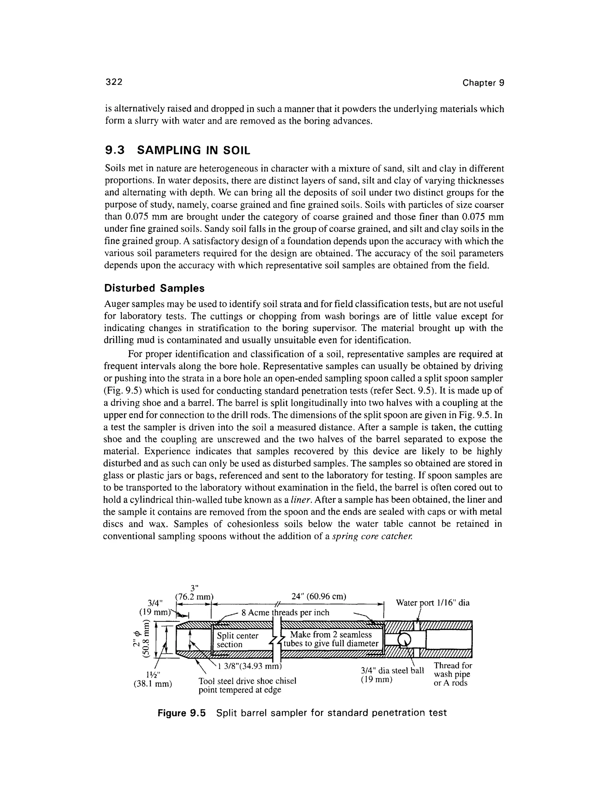
381. 362
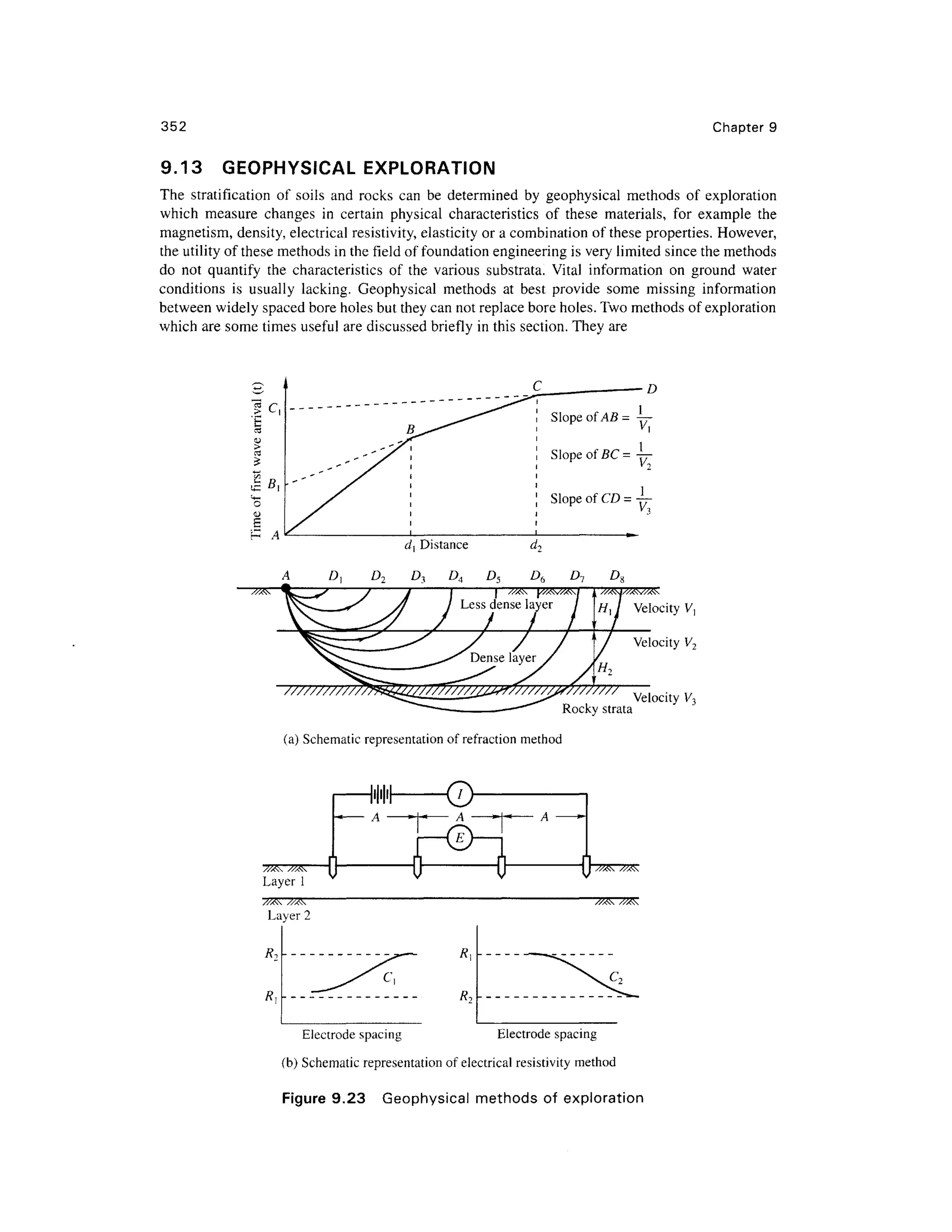
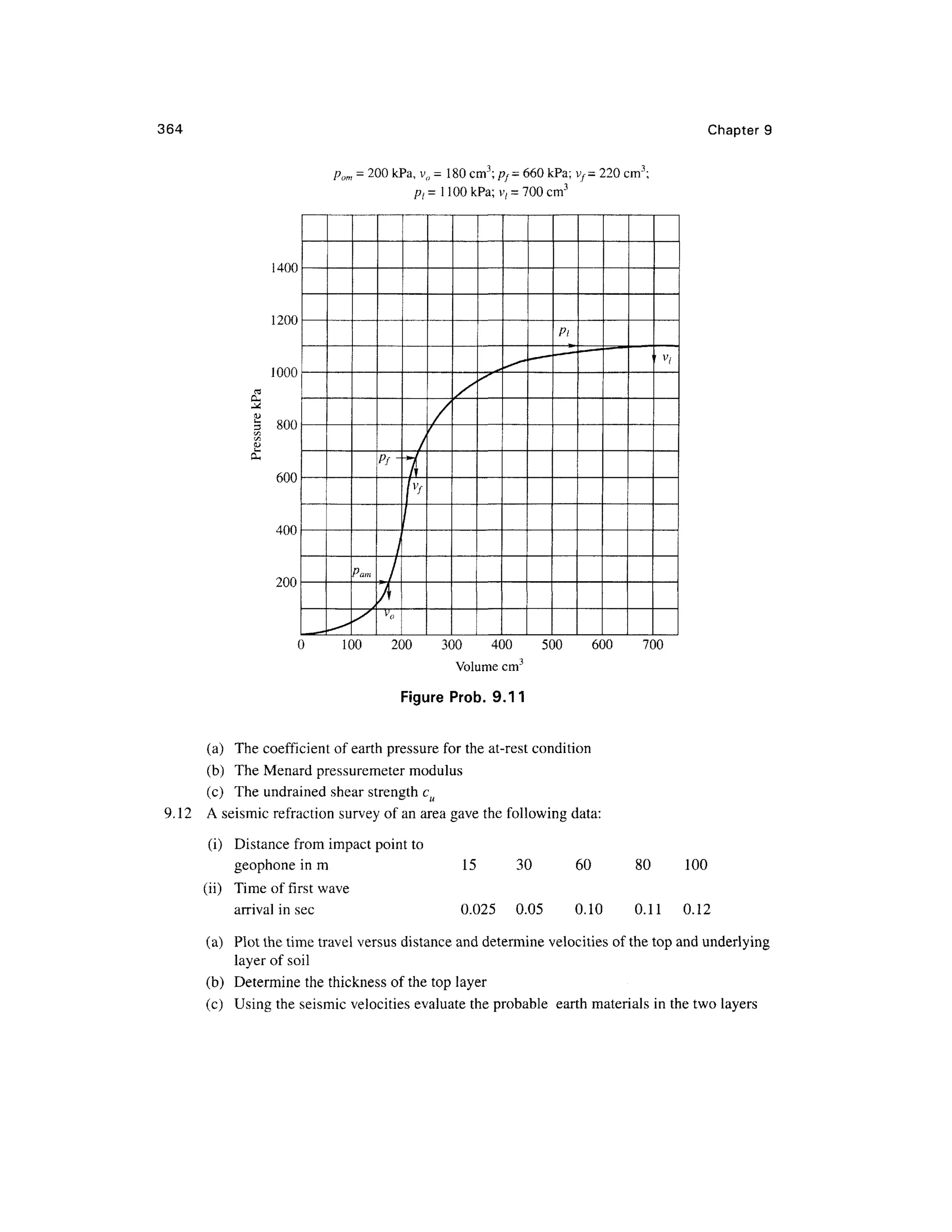
9.17 PROBLEM S
Chapter 9
9.1 Comput e the area ratio of a sampling tube given the outside diameter = 100 mm and inside
diameter = 94 mm. In what types of soil can this tube be used for sampling?
9.2 A standar d penetratio n tes t wa s carrie d ou t a t a site . Th e soi l profil e i s give n i n
Fig. Prob. 9.2 with th e penetration values. The average soi l data are given for each layer.
Compute the corrected value s of N and plot showing the
(a) variatio n of observed value s with depth
(b) variatio n of corrected value s with depth for standard energy 60 %
Assume: Eh = 0.7, C d = 0.9, C s = 0.85 an d Cb = 1.05
Depth (m)
0
2m
2-
Sand
•ysdt=185kN/m
3
•
4m
Figure Prob. 9. 2
N-values
20
A
8-
10-
1 9
14
'V ' . '. ' ' ' '
''-;'.- • ''• ;B ;• ''•:
'"' •"•' 'V - ?•'"••..'• ''".' i .'"•'•'-.v' : V
-'':
'..'' •'•'.' i .'"•''•'•.'J'' J
v•"• • : 'j.(- /•- .'.*•> * . ,v - V : 'i.^; .V
:
*y ... v - V ;'*; •
.7 ^y at = is 5 kN/m3
J'V'c ,•*'.;--•'•/-.- .'/"j;":^
Sand• -.;• • ••'.. :. ; ' . '.-.•' • ' . ; • . '
. :y sal= 1981kN/m3
:/ * . . •.,.'- . - :-.-'?. ,
. . C . . - . . . - ; • • - • • • '
,"
m
t-
m
m
[.'•'
. 3 0
' f " ^ *
/ /^ ]
CV
1 5
^ /''A/- ' 19
•
9.3 Fo r the soil profile given in Fig. Prob 9.2, compute the corrected values of W for standar d
energy 70% .
9.4 Fo r the soil profile given in Fig. Prob 9.2, estimate the average angle of friction for the sand
layers based o n the following:
(a) Tabl e 9.3
(b) E q (9.8 ) by assuming the profile contains less tha n 5% fines (Dr ma y b e taken fro m
Table 9.3 )
Estimate the values of 0 and Dr for 60 percent standar d energy.
Assume: Ncor = N6Q.
9.5 Fo r the corrected value s of W 60 given in Prob 9.2, determine the unconfined compressiv e
strengths o f cla y a t point s C an d D i n Fi g Pro b 9. 2 b y makin g us e o f Tabl e 9. 4 an d
Eq. (9.9). What is the consistency of the clay?
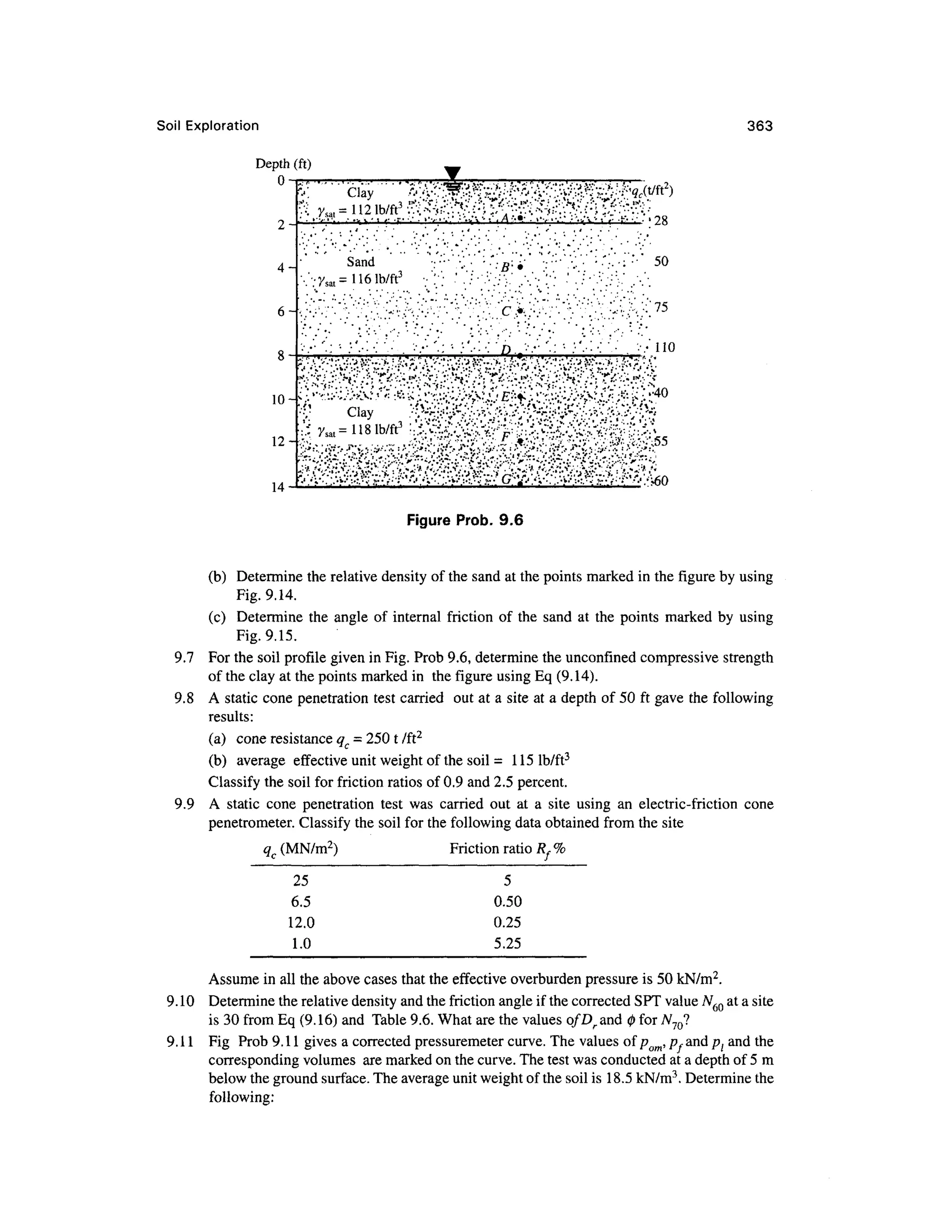
9.6 A stati c con e penetratio n tes t wa s carrie d ou t a t a sit e usin g a n electric-frictio n con e
penetrometer. Fig . Pro b 9. 6 give s th e soi l profil e an d value s o f q c obtained a t variou s
depths.
(a) Plo t the variation of q wit h depth

382. Soil Exploratio n 363
Depth (ft)
0
2-
Figure Prob. 9. 6
(b) Determin e the relative density of the sand at the points marked in the figure by using
Fig. 9.14 .
(c) Determin e th e angl e of internal friction of th e san d a t th e point s marke d b y using
Fig. 9.15 .
9.7 Fo r the soil profile given in Fig. Prob 9.6, determine the unconfmed compressive strength
of the clay at the points marked in th e figure using Eq (9.14).
9.8 A static cone penetration test carried ou t at a site at a depth of 50 ft gave the following
results:
(a) con e resistance qc = 250 t /ft2
(b) averag e effectiv e unit weight of the soil = 11 5 lb/ft3
Classify th e soil for friction ratios of 0.9 and 2.5 percent.
9.9 A stati c con e penetratio n tes t wa s carrie d ou t a t a sit e usin g an electric-frictio n con e
penetrometer. Classify the soil for the following data obtained from the site
q (MN/m 2
) Friction ratio Rf %
25
6.5
12.0
1.0
5
0.50
0.25
5.25
Assume in all the above cases that the effective overburden pressure is 50 kN/m2
.
9.10 Determin e the relative density and the friction angle if the corrected SPT value 7V60 at a site
is 30 from Eq (9.16) and Tabl e 9.6. What are the values o/Drand 0 for N JQ1
9.11 Fi g Pro b 9.11 gives a corrected pressuremete r curve. The values of pom, pf an d pl an d the
corresponding volumes ar e marked on the curve. The test was conducted at a depth of 5 m
below the ground surface. The average unit weight of the soil is 18.5 kN/m3
. Determine the
following:

383. 364 Chapter 9
1400
1200
1000
800
600
400
200
pom = 200 kPa, v0 = 180 cm3
; pf= 66 0 kPa; vf= 22 0 cm3
;
pt= 1100kPa;v / = 700cm3
Pan,
Pi
100 20 0 600 700
Figure Prob . 9.11
(a) Th e coefficient of earth pressure for the at-rest condition
(b) Th e Menard pressuremeter modulus
(c) Th e undrained shear strength cu
9.12 A seismic refraction survey of an area gave the following data:
(i) Distanc e from impac t point to
geophone i n m 1 5 3 0
(ii) Tim e of first wave
arrival in sec 0.02 5 0.0 5
60 80 100
0.10 0.1 1 0.1 2
(a) Plo t the time travel versus distance an d determine velocities of the top and underlying
layer of soil
(b) Determin e the thickness of the top layer
(c) Usin g the seismic velocities evaluate the probable eart h materials in the two layers

384. CHAPTER 10
STABILITY OF SLOPES
10.1 INTRODUCTIO N
Slopes of earth are of two types
1. Natura l slopes
2. Ma n made slopes
Natural slopes are those that exist in nature and are formed by natural causes. Suc h slopes
exist in hilly areas. The sides of cuttings, the slopes of embankments constructed for roads, railway
lines, canals etc. and the slopes of earth dams constructed for storing water are examples o f man
made slopes. The slopes whether natural or artificial may be
1. Infinit e slope s
2. Finit e slopes
The term infinite slope is used to designate a constant slope of infinite extent. The long slope
of the face of a mountain is an example of this type, whereas finite slopes are limited in extent. The
slopes of embankments and earth dams are examples of finite slopes. The slope length depends on
the height of the dam or embankment.
Slope Stability: Slop e stabilit y i s an extremely importan t consideration i n the desig n and
construction of earth dams. The stability of a natural slope is also important. The results of a slope
failure can often be catastrophic, involving the loss of considerable propert y and many lives.
Causes of Failure of Slopes: The important factors that cause instability in a slope and lead to
failure are
1. Gravitationa l force
2. Forc e due to seepage water
3. Erosio n of the surface of slopes due to flowing water
365

385. 366 Chapter 1 0
4. Th e sudden lowering of water adjacent to a slope
5. Force s due to earthquakes
The effec t o f al l the force s liste d above i s to cause movemen t o f soil fro m hig h points
to low points. The mos t importan t of such forces i s the component o f gravity that acts i n the
direction o f probable motion . The variou s effects of flowing or seepin g wate r ar e generally
recognized a s ver y importan t i n stabilit y problems, bu t ofte n thes e effect s hav e no t bee n
properly identified . It is a fact tha t the seepag e occurrin g withi n a soil mas s cause s seepag e
forces, whic h have much greater effec t than is commonly realized .
Erosion o n the surface of a slope ma y be the cause o f the removal o f a certain weigh t of
soil, an d may thu s lead to an increased stability as far as mass movement is concerned. O n the
other hand, erosion i n the form of undercutting at the toe may increase the height of the slope,
or decrease the length of the incipient failure surface , thus decreasing th e stability.
When there is a lowering of the ground water or of a freewater surface adjacent to the slope ,
for exampl e i n a sudden drawdown of the wate r surface i n a reservoir ther e i s a decrease i n th e
buoyancy of the soi l whic h is in effect a n increase i n the weight . This increas e i n weight cause s
increase i n th e shearin g stresse s tha t may o r may no t b e i n part counteracte d b y th e increas e in
Component of weight
C
Failure
surface
(a) Infinite slope (b) An earth dam
Ground
water table
Seepage
parallel to slope
(c) Seepage below a natural slope
Lowering of water
from leve l A to B
Earthquake
force
(d) Sudden drawdown condition (e ) Failure due to earthquake
Figure 10. 1 Force s that ac t o n earth slope s

386. Stability o f Slopes 36 7
shearing strength, depending upon whether or not the soil is able to undergo compression which the
load increas e tend s t o cause . I f a larg e mas s o f soi l i s saturate d an d i s o f lo w permeability ,
practically no volume changes will be able to occur except at a slow rate, and in spite of the increase
of load the strength increase may be inappreciable.
Shear at constant volume may be accompanied by a decrease i n the intergranular pressure
and an increase in the neutral pressure. A failure may be caused by such a condition in which the
entire soil mass passes into a state of liquefaction and flows like a liquid. A condition of this type
may be developed if the mass of soil is subject to vibration, for example, due to earthquake forces.
The various forces that act on slopes are illustrated in Fig. 10.1 .
10.2 GENERA L CONSIDERATION S AND ASSUMPTION S I N THE
ANALYSIS
There are three distinct parts to an analysis of the stability of a slope. They are:
1. Testing o f sample s to determin e the cohesio n and angle of internal friction
If the analysis is for a natural slope, it is essential that the sample be undisturbed. In such important
respects as rate of shear application and state of initial consolidation, the condition of testing must
represent as closely a s possible the most unfavorable conditions ever likely to occur in the actual
slope.
2. Th e study of items which ar e known to enter but which canno t b e accounted
for i n the computation s
The most important of such items is progressive crackin g which will start at the top of the slope
where the soil is in tension, and aided by water pressure, may progress to considerable depth . In
addition, ther e ar e th e effect s o f th e non-homogeneou s natur e o f th e typica l soi l an d othe r
variations from the ideal conditions which must be assumed.
3. Computatio n
If a slope is to fail alon g a surface, all the shearing strength must be overcome alon g that surface
which then becomes a surface of rupture. Any one such as ABC in Fig. 10.1 (b) represents one of an
infinite number of possible traces on which failure might occur.
It is assumed that the problem is two dimensional, which theoretically requires a long length
of slope normal to the section. However, if the cross section investigated holds for a running length
of roughly two or more times the trace of the rupture, it is probable that the two dimensional case
holds within the required accuracy.
The shear strength of soil is assumed to follow Coulomb's law
s = c' + dtan 0"
where,
c' - effectiv e uni t cohesion
d = effective norma l stress on the surface of rupture = (cr - u)
o -tota l normal stress on the surface of rupture
u - por e water pressure on the surface of rupture
0' = effective angle of internal friction.
The item of great importance is the loss of shearing strength which many clays show when
subjected to a large shearing strain. The stress-strain curve s for such clays show the stress rising
with increasing strai n to a maximum value, after whic h it decreases an d approaches a n ultimate

387. 368 Chapte r 1 0
value whic h ma y b e muc h les s tha n th e maximum . Sinc e a ruptur e surfac e tend s t o develo p
progressively rathe r than with all the points at the same stat e of strain, it is generally the ultimate
value that should be used for the shearing strength rather than the maximum value.
10.3 FACTO R O F SAFETY
In stability analysis, two types of factors of safety are normally used. They ar e
1. Facto r o f safety with respect t o shearing strength.
2. Facto r of safety with respect to cohesion. This is termed the factor of safety with respect to
height.
Let,
FS = facto r of safety with respect to strength
F, = facto r of safety with respect t o cohesion
FH = facto r of safety with respect t o height
F, = facto r of safety with respect t o friction
c'= mobilize d cohesio n
m
0' = mobilize d angle of friction
T= averag e valu e of mobilized shearing strength
s= maximu m shearing strength.
The factor of safety with respect to shearing strength, F5, may be written as
s c' + <j' tan<j)'
F
>=7 = ; -
The shearing strengt h mobilized at each point on a failure surface may be written as
c' .
T — _ _ L /T
i - LJ
S
F
,
or r= c;+<7'tan0 ; (10.2 )
c' ., tanfi
where c m -—, ta n fi
m = -
m
p Tm
p
Actually the shearing resistance (mobilized value of shearing strength) does not develop to a
like degree at all points on an incipient failure surface. The shearing strains vary considerably an d
the shearing stress may be far from constant. However the above expression i s correct o n the basis
of average conditions.
If the factors of safety with respect t o cohesion an d friction are different, we may write the
equation o f the mobilized shearin g resistance as
It wil l be show n late r o n that F, depends o n the height o f the slope. From thi s i t may be
concluded that the factor of safety with respect to cohesion ma y be designated a s the factoro f safety
with respect to height. This factor is denoted by FH and it is the ratio between the critical height and

388. Stability o f Slope s 36 9
the actual height, the critical height being the maximum height at which it is possible fo r a slope to
be stable. We may write from Eq. (10.3 )
(1Q4)
H
where F^ is arbitrarily taken equal to unity.
Example 10. 1
The shearing strengt h parameters o f a soil are
c' = 26.1 kN/m2
0' = 15°
c' = 17.8 kN/m2
Calculate the factor of safety (a) with respect to strength, (b) with respect to cohesion an d (c)
with respect to friction. The average intergranular pressure t f o n the failure surface is 102.5 kN/m2
.
Solution
On the basis of the given data, the average shearin g strengt h on the failure surface is
s = 26.7 + 102. 5 ta n 15°
= 26.7 + 102.5 x 0.268 = 54.2 kN/m2
and the average valu e of mobilized shearin g resistanc e i s
T= 17.8+ 102. 5 ta n 12°
= 17.8 + 102.5 x 0.212 = 39.6 kN/m 2
F - - . L26
39.6 17.8 0 ta n 0.21 2
The abov e exampl e show s th e facto r o f safet y wit h respect t o shea r strength , F s i s 1.37 ,
whereas th e factor s o f safet y wit h respec t t o cohesio n an d frictio n ar e different . Conside r tw o
extreme cases:
1 .Whe n the factor of safety with respect t o cohesion i s unity.
2. Whe n the factor of safety with respect t o friction is unity.
Casel
=26.70+ 102.50x0.268
9
12.9 0
Case 2
= 2.13
T= 39.60 = —— +102.50 tan 15C
F

389. 370 Chapte r 1 0
26.70
F
• + 27.50
c
12.1 0
We can have any combination of Fc and F, betwee n these two extremes cited above to give
the same mobilized shearing resistance of 39.6 kN/m2
. Some of the combinations of F cand F0 are
given below.
Combination of F c and F^
Fc 1.0 0 1.2 6 1.3 7 1.5 0 2.2 0
F0 2.1 2 1.5 0 1.3 7 1.2 6 1.0 0
Under Case 2, the value of Fc = 2.20 when F0 - 1.0 . The factor of safety F C = 2.20 is defined
as the, factoro f safety with respect to cohesion.
Example 10. 2
What will be the factors of safety with respect to average shearing strength, cohesion an d internal
friction o f a soil, for whic h the shear strengt h parameters obtaine d fro m the laboratory test s are
c' = 32 kN/m2
an d 0 ' = 18° ; th e expecte d parameter s o f mobilize d shearin g resistanc e ar e
c'm = 21 kN/m2
and 0' = 13° and the average effective pressure on the failure plane is 1 10 kN/m2
.
For the same value of mobilized shearing resistance determine the following:
1 .Facto r of safety with respect to height;
2. Facto r of safety with respect to friction whe n that with respect to cohesion i s unity; and
3. Facto r o f safety with respect to strength.
Solution
The availabl e shear strength of the soil is
s = 32 + 1 10 tan 18 ° = 32 + 35.8 = 67.8 kN/m 2
The mobilized shearing resistance of the soil is
T=21 + 11 0 tan 13 ° = 21 + 25.4 = 46.4 kN/m 2
_ 67. 8 . .,
Factor of safety with respect to average strength, r s = ——- 1-4 6
46.4
32
Factor o f safety wit h respect to cohesion,F C = — -= 1.52
_ _ ta n 18° _ 0.324 9 _
Factor o f safety with respect to friction,F<t> - ~ T T~ ~ ~ T T ~ n 2309
Factor of safety wit h respect to height, F H ( = Fc) will be at F0 = 1 .0
. , . 3 2 110tanl8 ° , . 3 2
i =46.4 = — + -
,therefore , F = -
= 3.0
Fc 1. 0 46.4-35. 8
Factor of safety with respect to friction a t F = 1 .0 is

390. Stability of Slope s 371
. , . 3 2 110tanl8 ° , . ^ 35. 8
r =46.
4 =
— + -
,therefore, F , = -
=2.49
1.0 F 0 * 46.4-3 2
Factor o f safety with respect t o strength Fs is obtained when FC = F+. We may write
32 11 0 tan 18°
or F=1.4
6
10.4 STABILIT Y ANALYSI S OF INFINITE SLOPES I N SAND
As an introduction to slope analysis, the problem of a slope of infinite extent is of interest. Imagine
an infinit e slope , a s show n i n Fig . 10.2, making a n angl e j 8 with th e horizontal . Th e soi l i s
cohesionless an d completely homogeneou s throughout . Then th e stresse s acting on any vertica l
plane in the soil are the same as those on any other vertical plane. The stress at any point on a plane
EF parallel to the surface at depth z will be the same as at every point on this plane.
Now consider a vertical slice of material ABCD havin g a unit dimension normal to the page.
The forces acting on this slice are its weight W, a vertical reaction R on the base of the slice, and two
lateral forces P{ actin g on the sides. Since the slice is in equilibrium, the weight and reaction ar e
equal i n magnitude and opposite i n direction. They hav e a common lin e o f action whic h passes
through the center of the base AB. The lateral forces must be equal and opposite an d their line of
action must be parallel to the sloped surface.
The normal and shear stresses o n plane AB are
a' = yzcos 2
fi
where cr' n = effective norma l stress ,
y =effective unit weight of the sand.
If full resistance is mobilized on plane AB, the shear strength, s, of the soil per Coulomb's law
is
s = af
n ta n 0'
when T= s, substituting for s and tf n, we have
Figure 10.2 Stabilit y analysi s of infinit e slope in sand

391. 372
or ta n /3 =tan 0'
Chapter 1 0
(10.5a)
Equation (10.5a) indicate s that the maximum value of (3 is limited to 0' if the slope i s to be
stable. Thi s conditio n hold s tru e for cohesionles s soil s whethe r th e slop e i s completel y dr y o r
completely submerged under water.
The factor of safety o f infinite slopes in sand may be written as
p =
tanfi (10.5b)
10.5 STABILIT Y ANALYSI S O F INFINITE SLOPE S I N CLA Y
The vertical stress<J v acting on plane AB (Fig . 10.3 ) where
av = yzcosfi
is represented b y OC in Fig. 10. 3 in the stress diagram. The normal stress on this plane is OE and
the shearing stress is EC. The line OC makes an angle (3 with the cr-axis .
The Mohr strength envelope is represented by line FA whose equation is
s = c' + cr'tan^'
According t o the envelope, the shearing strength is ED where the normal stres s is OE.
When /3 i s greater than 0' the lines OC and ED meet. In this case the two lines meet at A. As
long a s the shearing stres s on a plane is less than the shearing strengt h on the plane, ther e i s no
danger of failure. Figure 10. 3 indicates that at all depths at which the direct stress i s less than OB,
there is no possibility of failure. However at a particular depth at which the direct stress is OB, the
O E B
Figure 10. 3 Stabilit y analysi s of infinit e slopes i n clay soil s

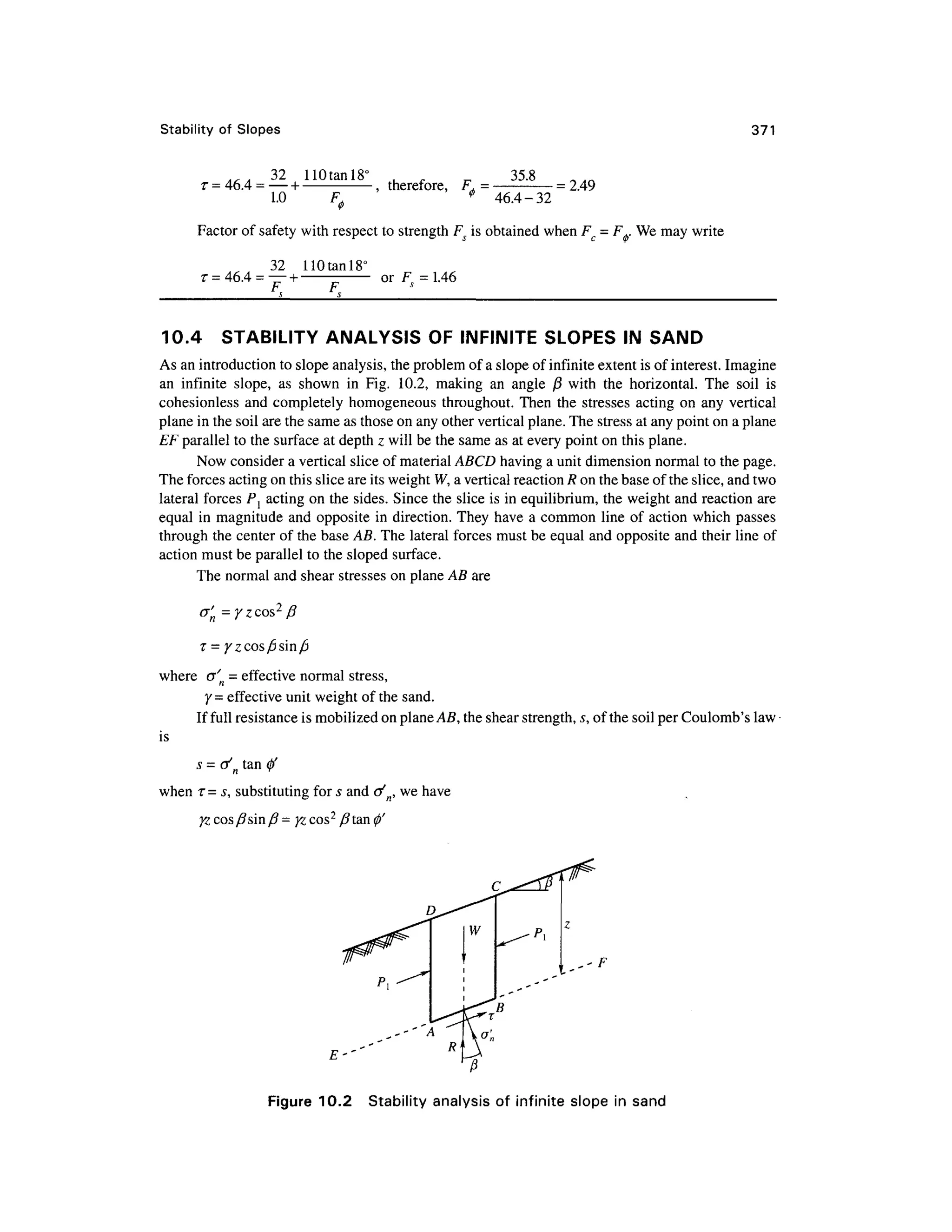
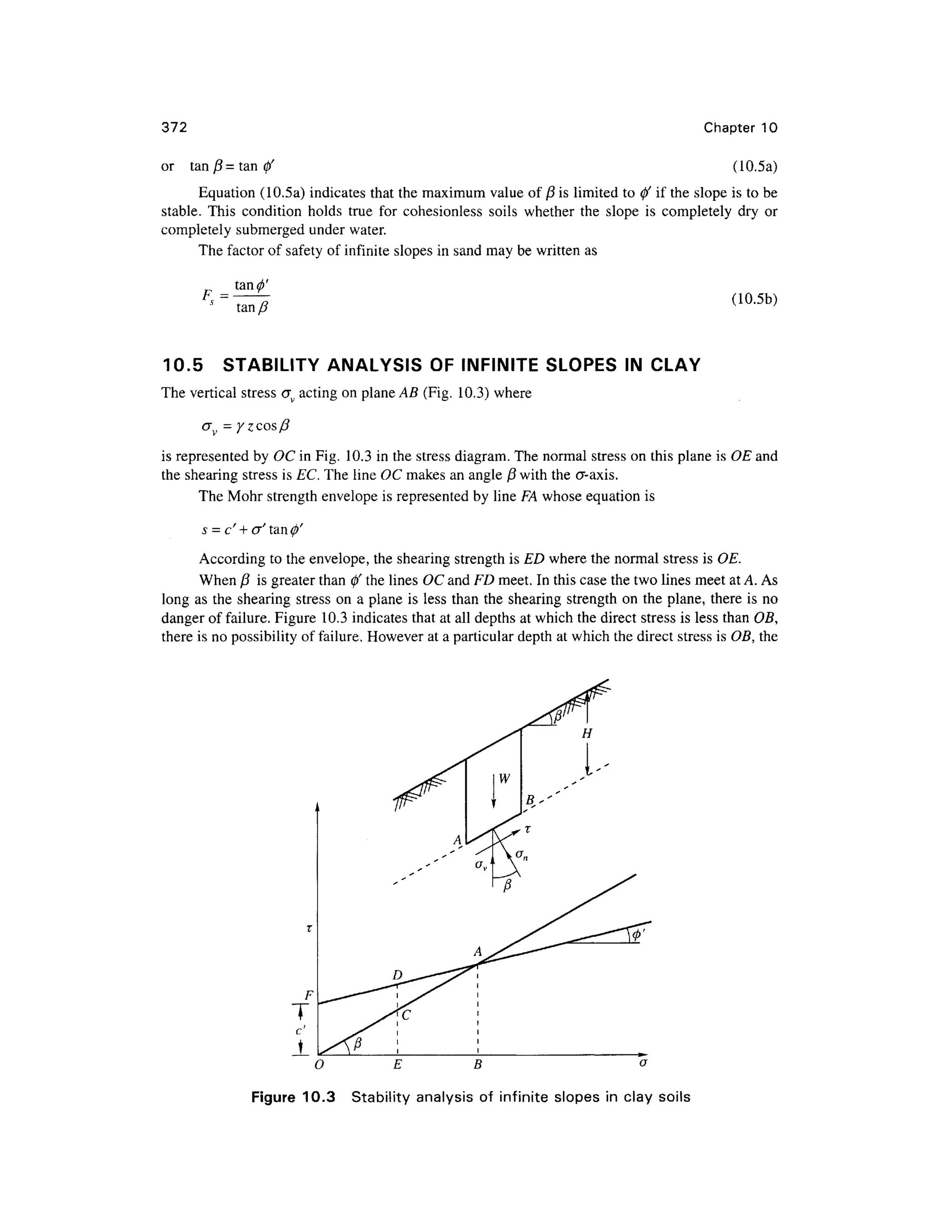
392. Stability of Slope s 37 3
shearing strength and shearing stres s value s are equal as represented b y AB, failur e i s imminent.
This depth at which the shearing stress and shearing strength are equal is called the critical depth.
At depths greater than this critical value, Fig. 10.3 indicates that the shearing stress is greater than
the shearing strength but this is not possible. Therefore it may be concluded that the slope may be
steeper tha n 0' as long as the depth of the slope is less than the critical depth.
Expression for th e Stabilit y of a n Infinite Slop e o f Cla y o f Dept h H
Equation (10.2) gives the developed shearin g stress as
T = c'm+(T'tan</>'m (10.6 )
Under conditions o f no seepage an d no pore pressure, the stress component s o n a plane at
depth H and parallel to the surface of the slope are
r=
<j' = yHcos 2
j3
Substituting these stress expressions i n the equation above and simplifying, we have
c'm = YHcos2
0 (tan 0 -tan 0'
J
c'
or N = ^
- = cos2
/?(tanytf-tan^) (10.7 )
yti
where H i s th e allowabl e heigh t an d th e ter m c'Jy H i s a dimensionless expressio n calle d th e
stability number and is designated a s A^. This dimensionless number is proportional to the required
cohesion and is inversely proportional to the allowable height. The solution is for the case when no
seepage is occurring. If in Eq. (10.7) the factor of safety with respect to friction is unity, the stability
number with respect t o cohesion ma y be written as
8)
, c
where c m= —
The stability number in Eq. (10.8) may be written as
where Hc = critical height. From Eq. (10.9), we have
Eq. (10.10) indicates that the factor of safety with respect to cohesion, Fc, is the same as the
factor of safety with respect t o height F H.
If there i s seepage parallel t o the ground surfac e throughout the entire mass , wit h the fre e
water surface coinciding with the ground surface, the components o f effective stresses o n planes
parallel to the surface of slopes at depth H are given as [Fig. 10.4(a)].
Normal stres s
(lO.lla)

393. 374 Chapter 1 0
(a)
(b)
Figure 10. 4 Analysi s of infinit e slope (a ) with seepage flow through the entir e
mass, and (b) with completely submerge d slope .
the shearing stress
T = ysatH si n /3 cos /3
Now substituting Eqs (10. 11 a) and (10. lib) into equation
(lO.llb)
and simplifying, th e stability expression obtained is
-^2— = cos2
0 ta n 0- -- tan</>'„
Y H Y
1
sat ' sat
(10.12)
As before, if the factor of safety with respect to friction i s unity, the stability number which
represents the cohesion may be written as
N= •
FY H Y H
c' sat 'sat ,
C/
= cos2
,tf tan^--^ -
' sat
(10.13)
If th e slop e i s completel y submerged , an d i f ther e i s n o seepag e a s i n Fig . 10.4(b) , the n
Eq. (10.13) become s
N = = cos2
/?(tan ft ~ tan<}>') (10.14)
where y , = submerged unit weigh t o f the soil.

394. Stability of Slope s 37 5
Example 10. 3
Find the factor of safety of a slope of infinite extent having a slope angle = 25°. The slope is made
of cohesionless soi l with 0 = 30°.
Solution
Factor o f safety
tan 30° 0.577 4
tan/? ta n 25° 0.466 3
Example 10. 4
Analyze the slope of Example 10. 3 if it is made of clay having c' - 3 0 kN/m2
, 0' =20°, e = 0.65 and
Gs = 2.7 and under the following conditions: (i) when the soil is dry, (ii) when water seeps parallel
to the surface of the slope, and (iii) when the slope is submerged.
Solution
For e = 0.65 and G = 2.7
= 27x^1 =
= (2. 7 +0.65)x9.81 =
ld
1 + 0.65 /sa t
1 +0.65
yb = 10.09 kN/m 3
(i) For dry soil the stability number Ns i s
c
N = ——— = cos2
/?(tan/?- tan<j>') whe n F,=l
' d c
= (cos 25° )2
(tan 25° -ta n 20°) = 0.084.
c' 3 0
Therefore, th e critical height H = -
= -
=22.25 m
16.05x0.084
(ii) For seepage parallel to the surface of the slope [Eq . (10.13)]
c' 100 Q
N = — -—= cos2
25° ta n 25°-^--
- tan 20° = 0.231 5
s
y tHc 19. 9
Hc=^= 3
°
= 6.5 1 m
c
y tNs 19.9x0.231 5
(iii) Fo r the submerged slope [Eq . (10.14)]
N = cos2
25° (tan 25° - ta n 20°) = 0.084
c
y bNs 10.09x0.08 4

395. 376 Chapte r 1 0
10.6 METHOD S O F STABILITY ANALYSIS OF SLOPES O F FINITE
HEIGHT
The stability of slopes o f infinite extent has been discussed in previous sections. A more commo n
problem is the one in which the failure occurs on curved surfaces. The most widely used method of
analysis of homogeneous, isotropic , finit e slope s i s the Swedish method base d o n circular failure
surfaces. Petterso n (1955 ) firs t applie d th e circl e metho d t o th e analysi s o f a soi l failur e i n
connection wit h th e failur e o f a quarr y wal l i n Goeteberg , Sweden . A Swedis h Nationa l
Commission, after studying a large number of failures, published a report in 192 2 showing that the
lines of failure of most such slides roughly approached th e circumference of a circle. The failure
circle might pass above the toe, through the toe or below it. By investigating the strength along the
arc o f a large numbe r of suc h circles, i t was possibl e to locate th e circl e whic h gave th e lowes t
resistance t o shear . Thi s genera l metho d ha s bee n quit e widel y accepte d a s offerin g a n
approximately correc t solutio n fo r th e determinatio n o f th e facto r o f safet y o f a slop e o f a n
embankment an d of its foundation. Developments in the method o f analysis have been mad e b y
Fellenius (1947) , Terzagh i (1943) , Gilboy (1934), Taylor (1937), Bisho p (1955), an d others, with
the resul t that a satisfactory analysis of the stability of slopes, embankment s and foundations by
means of the circle method is no longer an unduly tedious procedure.
There are other method s of historic interest such as the Culmann method (1875 ) and the
logarithmic spiral method. Th e Culman n metho d assume s tha t ruptur e wil l occu r alon g a
plane. I t is of interes t onl y as a classical solution, since actua l failure surfaces ar e invariably
curved. This method i s approximately correct fo r steep slopes. The logarithmic spira l metho d
was recommende d b y Renduli c (1935 ) wit h th e ruptur e surfac e assumin g th e shap e o f
logarithmic spiral . Thoug h thi s metho d make s th e proble m staticall y determinat e an d give s
more accurat e results , the greate r lengt h o f tim e required fo r computatio n overbalance s thi s
accuracy.
There are several methods of stability analysis based on the circular arc surface of failure. A
few o f the methods are described belo w
Methods o f Analysis
The majorit y o f the method s o f analysi s ma y be categorize d a s limit equilibriu m methods . Th e
basic assumptio n of the limit equilibrium approach i s that Coulomb's failur e criterion is satisfied
along the assumed failure surface. A free body is taken from the slope and starting from known or
assumed values of the forces acting upon the free body, the shear resistance of the soil necessary for
equilibrium i s calculated. Thi s calculate d shea r resistanc e i s then compared t o th e estimate d o r
available shear strength of the soil to give an indication of the factor of safety.
Methods tha t consider onl y the whole fre e bod y ar e the (a ) slope failur e under undrained
conditions, (b ) friction-circl e method (Taylor , 1937 , 1948 ) an d (c ) Taylor' s stabilit y numbe r
(1948).
Methods tha t divide the free body into many vertical slices an d consider the equilibrium of
each slic e ar e th e Swedis h circl e metho d (Fellenius , 1927) , Bisho p metho d (1955) , Bisho p and
Morgenstern metho d (1960 ) an d Spence r metho d (1967) . Th e majorit y of thes e method s ar e in
chart form and cover a wide variety of conditions.
10.7 PLAN E SURFACE OF FAILURE
Culmann (1875 ) assumed a plane surface of failure for the analysis of slopes which is mainly of
interest because i t serves as a test of the validity of the assumption of plane failure. In some cases
this assumption is reasonable an d in others it is questionable.

396. Stability of Slope s 377
Force triangle
Figure 10. 5 Stabilit y of slope s b y Culman n metho d
The method a s indicated abov e assumes tha t the critical surfac e of failure is a plane surface
passing through the toe of the dam as shown in Fig. 10.5 .
The forces that act on the mass above trial failure plane AC inclined at angle 6 with the horizontal are
shown in the figure. The expression for the weight, W, and the total cohesion C are respectively,
W = -yLHcosec /? sin(jtf- 0)
The use of the law of sines in the force triangle, shown in the figure, give s
C _ sm(6>-f )
W ~ cos^ '
Substituting herein for C and W, and rearranging we have
1
in which the subscript Q indicates tha t the stability number is for the trial plane at inclination 6.
The most dangerous plane is obtained by setting the first derivative of the above equatio n
with respect t o Q equal to zero. This operation give s
where & 'ci s th e critica l angl e fo r limitin g equilibriu m an d th e stabilit y numbe r fo r limitin g
equilibrium may be written as
yHc 4 sin/? cos 0'
where H i s the critical heigh t of the slope.
(10.15)

397. 378 Chapte r 10
If we write
F -— F tan
^'
c
~V' < > ~ t a n ^
where Fc an d F^ ar e safety factors wit h respect t o cohesion an d friction respectively, Eq . (10.15)
may be modified for chosen values of c an d 0' a s
^=
4 sin/3 cos(/)'m (10.16 )
The critical angle for any assumed values of c'm and 0'm is
1
From Eq . (10.16), th e allowable height of a slope is
Example 10.5
Determine by Culmann's method the critical height of an embankment having a slope angle of 40°
and the constructed soil having c' = 630 psf, 0' = 20° and effective uni t weight =114 lb/ft3
. Find the
allowable height of the embankment if F, = F, = 1 .25.
Solution
4c'sin/?cos0' 4 x 630 x sin 40° cos 20°
H, = -
- -
—= -
= 221 ft
y[l-cos(0-4>')] 114(l-cos20° )
For F c = F.= 1.25, c '= —= —= 504 lb/ft2
<(> m
' ta n 20°
and ta n #, = —- = — —= 0.291, f a = 16.23°
,, , • , 4x50 4 sin 40° cos 16.23° ^ 0 r
Allowable height, H = -
=128.7 ft.
_ 114[l-cos(40 - 16.23°)]
10.8 CIRCULA R SURFACES OF FAILURE
The investigation s carried ou t in Sweden a t the beginning of this century have clearly confirme d
that the surfaces of failure of earth slopes resemble the shape of a circular arc. When soil slips along
a circula r surface , suc h a slid e ma y b e terme d a s a rotational slide . I t involve s downward an d
outward movement of a slice of earth as shown in Fig. 10.6(a) and sliding occurs alon g the entire
surface of contact between th e slice and its base. The types of failure that normally occur may be
classified a s
1. Slop e failure

398. Stability o f Slope s 37 9
2. To e failure
3. Bas e failure
In slope failure, the arc of the rupture surface meets the slope above the toe. This can happen
when the slope angle /3 is quite high and the soil close to the toe possesses high strength. Toe failure
occurs when the soil mass of the dam above the base and below the base is homogeneous. The base
failure occurs particularly when the base angle j3 is low and the soil below the base is softer and
more plastic than the soil above the base. The various modes of failure are shown in Fig. 10.6 .
Rotational
slide
(a) Rotational slide
(b) Slope failur e
(c) Toe failure
(d) Base failure
Figure 10. 6 Type s of failur e o f eart h dams

399. 380 Chapter 1 0
10.9 FAILUR E UNDER UNDRAINE D CONDITION S (0 M = 0 )
A full y saturate d cla y slop e ma y fai l unde r undraine d condition s (0 u = 0 ) immediatel y afte r
construction. The stability analysis is based on the assumption that the soil is homogeneous and the
potential failure surface is a circular arc. Two types of failures considered ar e
1. Slop e failure
2. Bas e failure
The undraine d shear strength cu of soil is assumed t o be constant with depth. A trial failure
circular surfac e AB with center at 0 an d radius R is shown in Fig. 10.7(a ) for a toe failure. The slope
AC and the chord AB make angles /3 and a with the horizontal respectively. W is the weight per unit
Firm bas e
(a) Toe failur e (b) Base failure
Figure 10. 7 Critica l circl e position s fo r (a ) slope failure (afte r Fellenius , 1927) , (b )
base failur e
1>
50C
40C
20°
10
90C
70°
Values of
(a)
60C
50° 50 40° 30 ° 20 °
Values o f?
10° 0°
Figure 10. 8 (a ) Relation betwee n slop e angle / 3 and parameter s a and Q for
location o f critica l to e circl e whe n /3 i s greater than 53° ; (b ) relation betwee n slope
angle /3 an d depth facto r n d for variou s value s o f paramete r nx
(after Fellenius , 1927 )

400. Stability of Slope s 38 1
length of the soil lying above the trial surface acting through the center of gravity of the mass. lo is
the leve r arm , La i s th e lengt h of the arc , L c th e lengt h o f th e chor d AB an d c m th e mobilize d
cohesion for any assumed surface of failure.
We may express the factor of safety F^ as
(10.19)
For equilibrium of the soil mass lying above the assumed failure surface, we may write
resisting moment Mr = actuating moment Ma
The resisting moment Mf = LacmR
Actuating moment, Ma = Wlo
Equation for the mobilized c i s
W10
(10.20)
Now th e facto r o f safet y F fo r th e assume d tria l ar c o f failur e may b e determine d fro m
Eq. (10.19). This is for one trial arc. The procedure has to be repeated for several trial arcs and the
one that gives the least value is the critical circle.
If failure occurs along a toe circle, the center of the critical circle can be located by laying off
the angles a and 26 as shown in Fig. 10.7(a) . Values of a and 6 for different slop e angles /3 can be
obtained from Fig. 10.8(a) .
If there is a base failure as shown in Fig. 10.7(b), the trial circle will be tangential to the firm
base and as such the center of the critical circle lies on the vertical line passing through midpoint M
on slope AC. The following equations may be written with reference to Fig. 10.7(b) .
D x
Depth factor, n d = — , Distanc e factor, nx = — (10.21 )
H H
Values o f n x ca n b e estimate d fo r differen t value s o f n d an d j 8 by mean s o f th e char t
Fig. 10.8(b) .
Example 10. 6
Calculate th e facto r of safet y agains t shea r failur e along th e sli p circl e show n in Fig. Ex . 10. 6
Assume cohesion = 40 kN/m2
, angl e of internal friction = zero and th e total uni t weight of the
soil = 20.0 kN/m3
.
Solution
Draw the given slope ABCD as shown in Fig. Ex. 10.6. To locate the center of rotation, extend the
bisector o f line BC to cut the vertical line drawn from C at point O. With O as center and OC as
radius, draw the desired sli p circle.
2
Radius OC =R=36.5 m, Area BECFB = - xEFxBC
2
= - x 4 x32.5 = 86.7 m2
Therefore W = 86.7 x 1 x 20 = 1734 kN
W acts through point G which may be taken as the middle of FE.

401. 382 Chapter 1 0
s
s R = 36.5m
Figure. Ex . 10. 6
From the figure we have, x = 15.2 m, and 9= 53°
3.14
Length of arc EEC =R0= 36.5 x 53° x —— = 33.8 m
180
length of arc x cohesion x radius 33.8x40x36. 5
Wx 1734x15.2
10.10 FRICTION-CIRCL E METHO D
Physical Concept o f the Metho d
The principl e o f th e metho d i s explained wit h reference t o the sectio n throug h a dam show n in
Fig. 10.9 . A trial circle with center of rotation O is shown in the figure. With center O and radius
Friction circle
Trial circular
failure surface
Figure 10. 9 Principl e of friction circle method

402. Stability of Slope s 383
sin 0", where R is the radius of the trial circle, a circle is drawn. Any line tangent to the inner circle
must intersec t th e tria l circl e a t a n angl e t f wit h R . Therefore , an y vecto r representin g a n
intergranular pressure at obliquity 0' to an element of the rupture arc must be tangent to the inner
circle. This inner circle is called the frictioncircle or ^-circle. The friction circl e method of slope
analysis is a convenient approach for both graphical an d mathematical solutions . It is given this
name because the characteristic assumptio n of the method refers to the 0-circle.
The forces considered i n the analysis are
1. Th e total weight W of the mass above the trial circle acting through the center of mass. The
center of mass may be determined by any one of the known methods.
2. Th e resultant boundary neutral force U. The vector U may be determined b y a graphical
method from flownet construction.
3. Th e resultant intergranular force, P, acting on the boundary.
4. Th e resultant cohesive force C.
Actuating Force s
The actuating forces may be considered to be the total weight W and the resultant boundary force U
as shown in Fig. 10.10 .
The boundary neutral force always passes through the center of rotation O. The resultant of W
and U , designated as Q, is shown in the figure.
Resultant Cohesiv e Forc e
Let the length of arc AB be designated as La, the length of chord AB by Lc. Let the arc length La be
divided into a number of small elements and let the mobilized cohesive force on these elements be
designated as Cr C2, C3, etc. as shown in Fig. 10.11 . The resultant of all these forces is shown by
the force polygon in the figure. The resultant is A'B' which is parallel and equal to the chord length
AB. The resultant of all the mobilized cohesional force s along the arc is therefore
C = c'L
Figure 10.1 0 Actuatin g forces

403. 384 Chapter 1 0
(a) Cohesiv e forces o n a trial arc (b ) Polygo n of forces
Figure 10.1 1 Resistan t cohesiv e force s
We may write c' m - —
c
wherein c'= unit cohesion, F C = factor of safety with respect t o cohesion.
The line of action of C may be determined by moment consideration. The moment of the total
cohesion i s expressed a s
c' L R = c' L I
m a m c a
where l = moment arm. Therefore ,
(10.22)
It is seen that the line of action of vector C is independent of the magnitude of c' m
.
Resultant o f Boundar y Intergranula r Force s
The trial arc of the circle is divided into a number of small elements. Let Pv P2, Py etc . b e the
intergranular force s actin g on these elements a s shown in Fig. 10.12 . The friction circl e i s drawn
with a radius of R sin (j/ m
where
The lines of action of the intergranular forces Pr P2, Py etc . are tangential to the friction
circle an d mak e a n angl e o f 0' m a t the boundary . However, th e vecto r su m o f an y tw o smal l
forces ha s a lin e o f actio n throug h poin t D , missin g tangenc y t o th e 0' m-circle b y a smal l
amount. The resultant of all granular forces mus t therefore mis s tangenc y to the 0'm-circle by
an amount whic h is not considerable. Le t the distance o f the resultant of the granular force P
from th e cente r o f th e circl e b e designate d a s K R si n 0 ' (a s show n i n Fig . 10.12) . Th e

404. Stability of Slope s 385
KRsin<p'n
Figure 10.1 2 Resultan t o f intergranula r force s
magnitude of K depends upon the type of intergranular pressure distributio n along the arc. The
most probable for m o f distribution i s the sinusoidal distribution .
The variation of K with respect to the central angle a'is shown in Fig. 10.13 . The figure also
gives relationship s betwee n of an d K fo r a uniform stres s distributio n of effective norma l stres s
along the arc of failure.
The graphical solution based on the concepts explained above is simple in principle. For the
three forces Q, C and P of Fig. 10.1 4 to be in equilibrium, P must pass through the intersection of
1.20
1.16
1.12
1.08
1.04
1.00
ox
£
^
71
str
^
Cent
For i
essc
/
ral angle
anifo
istrih
/
^
rm
>utior
j
/
s<
i —S
/
/
/
s
/
y
/
For
tress
/
'
/
sinus
distr
/
/
/
oida
ibuti(
J
/
^n
20 4 0 6 0 8 0
Central angle a ' in degrees
100 120
Figure 10.1 3 Relationshi p betwee n K and central angl e a'

405. 386 Chapter 1 0
Figure 10.1 4 Forc e triangle fo r th e friction-circl e metho d
the known lines of action of vectors Q and C. The line of action of vector P must also be tangent to
the circl e o f radius KR si n 0' . The valu e of K may b e estimate d b y the us e of curves give n in
Fig. 10.13 , and the line of action offeree P may be drawn as shown in Fig. 10.14 . Since the lines of
action of all three forces and the magnitude of force Q are known, the magnitude of P and C may-be
obtained by the force parallelogram construction that is indicated in the figure. The circle of radius
of KR sin 0' i s called the modified friction circle.
T
rn j j
Determination of Facto r o f Safet y With Respec t to Strengt h
Figure 10.15(a ) is a section o f a dam. AB is the trial failure arc. The force Q , the resultant of W
and U is drawn as explained earlier. The line of action of C is also drawn. Let the forces Q and C
D
(a) Friction circle (b) Facto r of safet y
Figure 10.1 5 Graphica l method of determining factor o f safet y wit h respect t o
strength

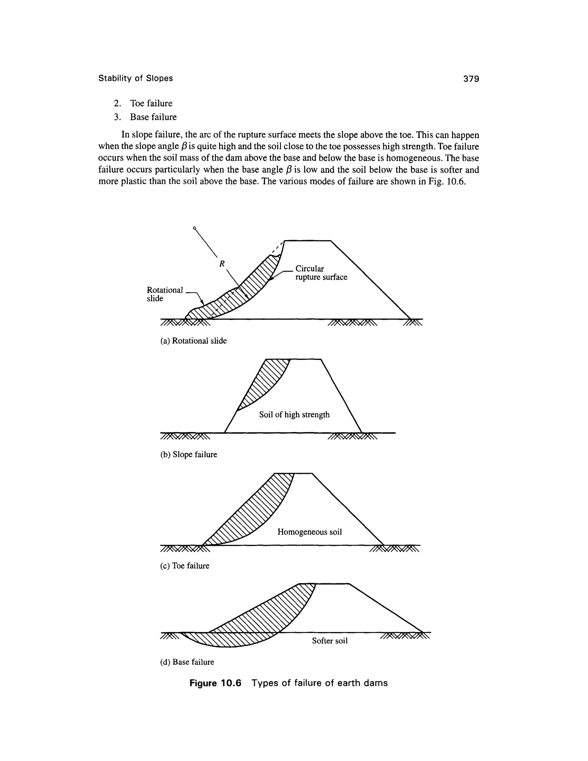
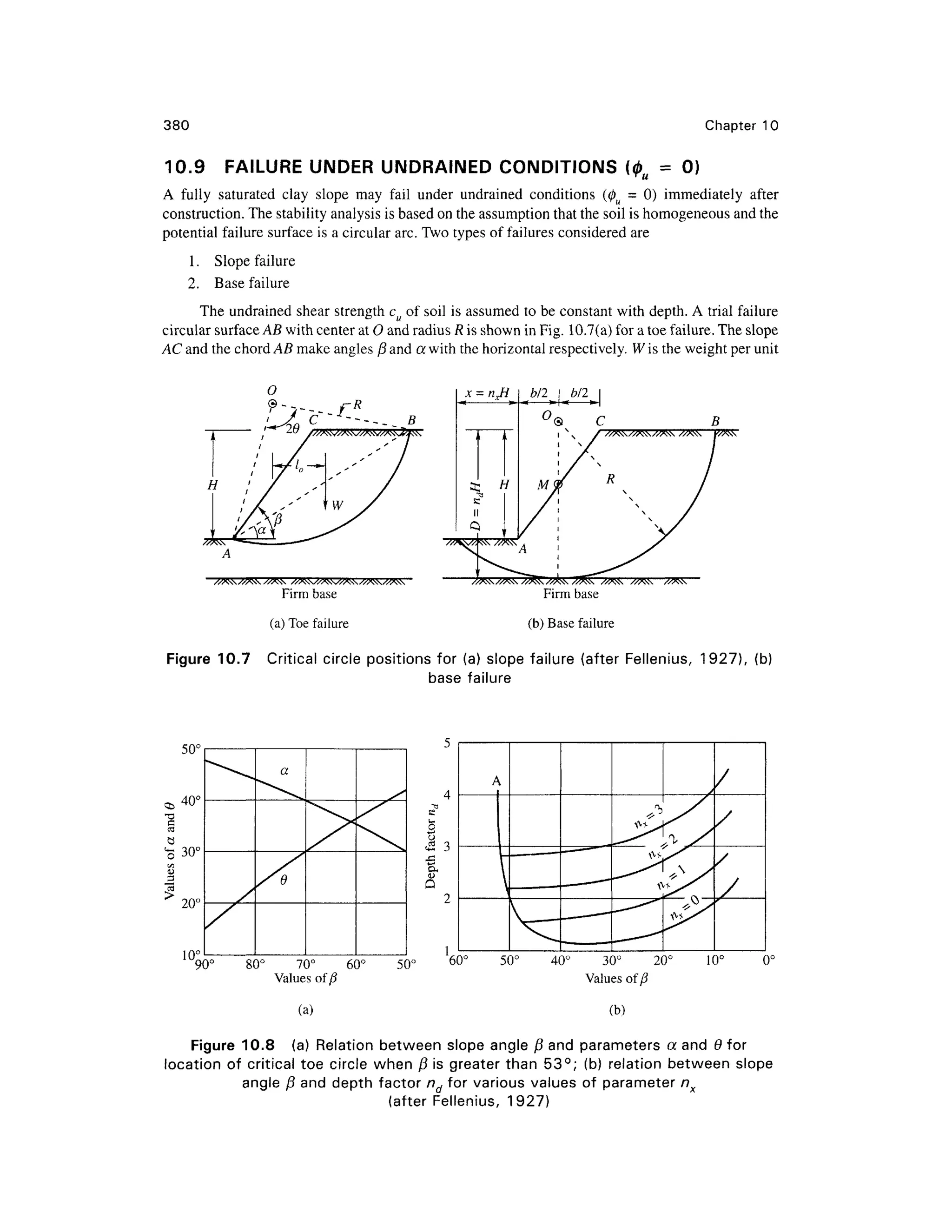
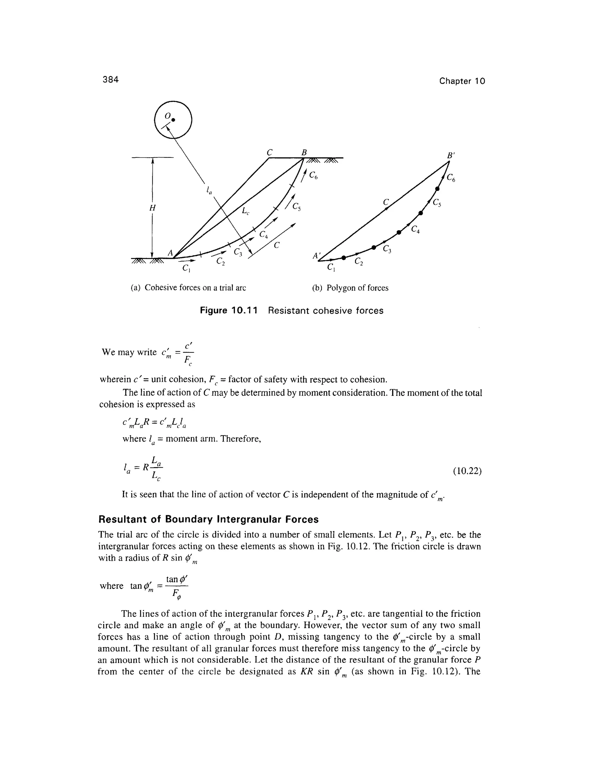
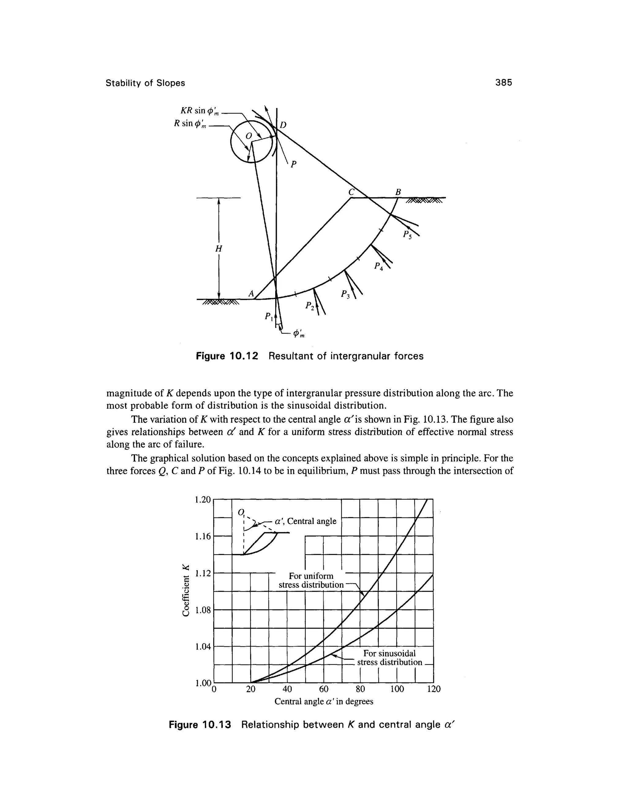
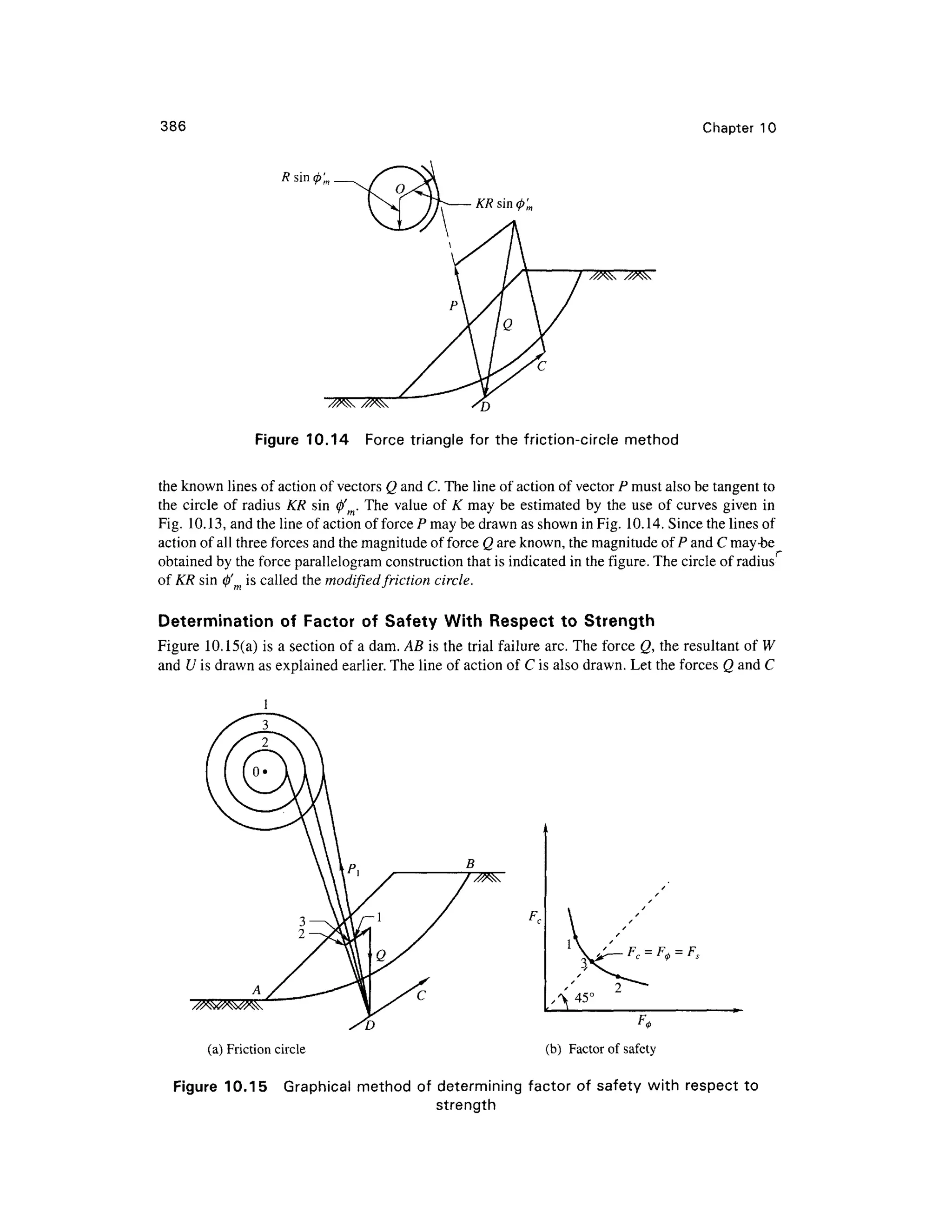
406. Stability o f Slope s 38 7
meet at point D. An arbitrary first trial using any reasonable $m value, which will be designated
by 0' ml i s given by th e us e o f circle 1 or radius KR si n <j)' ml. Subscrip t 1 is used fo r al l other
quantities of the first trial. The force Pl is then drawn through D tangent to circle 1 . Cl is parallel
to chord an d point 1 is the intersection of forces C { an d Pr Th e mobilized cohesio n i s equal
c'm]Lc. From thi s the mobilized cohesion c'ml i s evaluated. The factors of safety with respect to
cohesion and friction are determined from the expressions
c' tanfl'
F' = ——, an d F*,
These factors are the values used to plot point 1 in the graph in Fig. 10.15(b) . Similarly
other friction circles wit h radii KR sin <j/ m2, K R sin 0'm3. etc. may be drawn and the procedur e
repeated. Point s 2, 3 etc. ar e obtained as shown in Fig. 10.15(b). The 45° line , representing
Fc = F.,intersects the curve to give the factor of safety Fs for this trial circle.
Several trial circles must be investigated in order to locate the critical circle, which is the one
having the minimum value of F5.
Example 10.7
An embankment has a slope of 2 (horizontal) to 1 (vertical) with a height of 10 m. It is made of a
soil havin g a cohesio n o f 3 0 kN/m 2
, a n angl e o f interna l friction o f 5 ° an d a uni t weigh t of
20 kN/m3
. Consider any slip circle passing through the toe. Use the friction circle method to find
the factor of safety with respect to cohesion.
Solution
Refer to Fig. Ex. 10.7 . Let EFB be the slope and AKB be the slip circle drawn with center O and
radius R = 20 m.
Length of chord AB = Lc = 27 m
Take J as the midpoint of AB, then
Area AKBFEA = area AKBJA + area ABEA
= -ABxJK + -ABxEL
3 2
= -x27 x 5.3 + -x 27 x 2.0 =122.4 m2
3 2
Therefore th e weight of the soil mass = 122. 4 x 1 x 20 = 2448 kN
It will act through point G, the centroid of the mass which can be taken as the mid point of
FK.
Now, 0= 85° ,
314
Length of arc AKB = L = RO = 20 x 85 x—= 29.7 m
6
18 0
L 29. 7
Moment arm of cohesion, / = R— = 20 x —— = 22 m
L
c 21
From cente r O , at a distance / fl, dra w the cohesive force vector C , which is parallel to the
chord AB. Now from the point of intersection of C and W, draw a line tangent to the friction circle

407. 388 Chapter 1 0
1.74m
//=10m
Figure Ex. 10. 7
drawn at 0 wit h a radius of R sin 0' = 20 sin 5° = 1 .74 m. This line is the line of action o f the third
force F.
Draw a triangle of forces in which the magnitude and the direction fo r W is known and only
the directions o f the other two forces C and F are known.
Length ad gives the cohesive force C = 520 kN
Mobilized cohesion ,
c' = -
= —= 17.51 kN/m2
m
L 29. 7
Therefore the factor of safety with respect t o cohesion, Fc, is
F =11 =
^=1.713
FC will be 1 .7 13 if the factor of safety with respect to friction, F^ - 1 .0
tan5c
If, F = 1.5, the n 0' =
F.
= 0.058 rad; o r 0' = 3.34°

408. Stability of Slope s 38 9
The new radius of the friction circl e is
r{ = Rsin 0'm = 20 x sin 3.3° = 1.16 m.
The direction of F changes and the modified triangle of force abd' gives ,
cohesive force = C = length ad' = 600 kN
C 60 0
Mobilised cohesino, c' m = ~— - - 20. 2 kN/mr
LJ Z*yI /
c' 3 0
Therefore, F = — =
= 1.5
c
c' 20. 2
10.1 1 TAYLOR' S STABILIT Y NUMBE
R
If th e slop e angl e j8 , height o f embankmen t H , th e effectiv e unit weight o f materia l y , angle o f
internal friction</>' , and unit cohesion c' are known, the factor of safety may be determined. I n order
to make unnecessary the more or less tedious stability determinations, Taylor (1937) conceived th e
idea of analyzing the stability of a large number of slopes through a wide range of slope angles and
angles of internal friction, and then representing the results by an abstract number which he called
the "stability number". This number is designated as A^. The expression use d is
From this the factor of safety with respect to cohesion ma y be expressed a s
F
- = 7 < 10
-24
>
Taylor published his results in the form of curves which give the relationship between Ns and
the slop e angle s / ? for variou s values of 0 ' as shown in Fig. 10.16 . These curves ar e for circle s
passing throug h the toe , althoug h for value s of 13 less tha n 53°, i t has bee n foun d that th e mos t
dangerous circle passes below the toe. However, these curves may be used without serious error for
slopes dow n to fi = 14° . The stabilit y numbers are obtained fo r factor s of safety wit h respect t o
cohesion b y keeping th e factor of safety with respect t o friction (FJ equal to unity.
In slopes encountered in practical problems, the depth to which the rupture circle may extend
is usually limited by ledge or other underlying strong material as shown in Fig. 10.17 . The stability
number Ns fo r the case when 0 " = 0 is greatly dependent on the position of the ledge. The depth at
which the ledge or strong material occurs may be expressed i n terms of a depth factor nd which is
defined a s
»rf=;| (10-25 )
where D - dept h of ledge below the top of the embankment, H = height of slope above the toe.
For various value s o f nd an d for the 0 = 0 case th e char t i n Fig. 10.1 7 give s th e stabilit y
number NS fo r various values of slope angle ft. In this case the rupture circle may pass through the
toe o r belo w th e toe . Th e distanc e j c of th e ruptur e circle fro m th e to e a t th e to e leve l ma y b e
expressed b y a distance factor n whic h is defined as

409. •a
Stability
number
,
N
s
CD
H
°
|_cu
o
a
cr
-*
C
D
<°
o
^
^
C
CD
_j
O
O)
0)
o"
V)*
Q)
CT
(Q
C
Stability
number,
N,.
Q)
-.
<.
Q)
O
—
f
>
-
i
r-t-
>
CD
c
n
~"
w
—
J
r-
+
Q)
0
)
<
.
E
o
^
~
CD
C
co
3
->J
c
r
'**
CD
-^
cn
oee

410. Stability of Slope s 39 1
The chart in Fig. 10.1 7 shows the relationship between nd and nx. If there is a ledge or other
stronger material at the elevation of the toe, the depth factor nd for this case is unity.
Factor o f Safet y with Respec t to Strengt h
The development of the stability number is based o n the assumption that the factor of safety with
respect t o frictio n F,, i s unity . The curve s giv e directly th e facto r o f safet y F c wit h respect t o
cohesion only . If a true factor of safety Fs wit h respect t o strength is required, this factor should
apply equall y t o bot h cohesio n an d friction . Th e mobilize d shea r strengt h ma y therefor e b e
expressed as
s c ' a' tan(/)'
In the above expression, we may write
— = c'm, ta n(f>'m = —=—, o r # , = — (approx. ) (10 .27)
S 5 S
c'm and tf m may be described a s average values of mobilized cohesion and friction respectively.
Example 10. 8
The following particulars are given for an earth dam of height 39 ft. The slope is submerged and the
slope angle j3 =45°.
Yb = 69 lb/ft 3
c' = 550 lb/ft 2
0' = 20°
Determine the factor of safety FS.
Solution
Assume as a first trial Fs = 2.0
20
<t>'m
=
Y =
10
° (approx. )
For (j)' m = 10°, and (3 = 45° th e value of Ns fro m Fig. 10.1 6 is 0.1 1, we may writ e
c'
From Eq. (10.23) N = -
,substituting
55Q
2x69x#
or H = — = 36.2 3 ft
2x69x0.11
20
If F = 1.9, $= —= 10.53° and N = 0.105
5
1 9 *

411. 392 Chapte r 1 0
.40ft
1.9x69x0.105
The computed heigh t 40 ft is almost equal to the given height 39 ft. The computed factor of
safety i s therefore 1 .9.
Example 10. 9
An excavation is to be made in a soil deposit with a slope of 25° to the horizontal and to a depth of
25 meters. The soil has the following properties:
c'= 35kN/m2
, 0' = 15° and 7= 2 0 kN/m3
1 . Determin e the factor of safety of the slope assuming full frictio n i s mobilized.
2. I f the factor of safety wit h respect t o cohesion i s 1.5 , what would be th e factor of safety
with respect to friction?
Solution
1 .Fo r 0' = 15° and (3 = 25°, Taylor's stability number chart gives stability number Ns = 0.03.
-233
0.03x20x25
2. Fo r F = 1.5, N = -
- -
- -
— -
=0.047
J
F cxyxH 1.5x20x2 5
For A^ = 0.047 and (3 = 25°, we have from Fig. 10.16 , 0'm = 13
tan0' ta n 15° 0.26 8
Therefore, F , = -
—= -
= -
=1.16
0
tan 0 ta n 13° 0.23 1
Example 10.1 0
An embankment i s to be made from a soil having c' = 420 lb/ft 2
, 0 ' = 18 ° and y= 12 1 lb/ft3
. Th e
desired facto r o f safet y wit h respec t t o cohesio n a s wel l a s tha t wit h respect t o frictio n i s 1.5 .
Determine
1 . Th e safe height if the desired slope is 2 horizontal to 1 vertical.
2. Th e saf e slope angle if the desired height is 50 ft.
Solution
, 0.32 5
tan 0' = ta
n 18° =0.325, 0' m - ta n ' — -
= 12.23°
1. Fo r 0' = 12.23 ° an d (3 =26.6° (i.e. , 2 horizontal and 1 vertical) the chart give s Ns = 0.055
c' 42 0
Therefore, 0.05 5 =
FcyH1. 5 x121 x H

412. Stability o f Slopes 393
Therefore, # . =
420
2. Now , NS = •
safe
1.5x121x0.05 5
420
= 42 ft
= 0.046
FcyH 1.5x121x5 0
For N = 0.046 and 0' = 12.23°, slope angle P = 23.5C
10.12 TENSIO N CRACKS
If a dam is built of cohesive soil, tension cracks are usually present at the crest. The depth of such
cracks may be computed from the equation
r (10.28)
where z0 = depth of crack, c ' = unit cohesion, y = unit weight of soil.
The effective length of any trial arc of failure is the difference between the total length of arc
minus the depth of crack as shown in Fig. 10.18.
10.13 STABILIT Y ANALYSIS B Y METHOD O F SLICES FOR
STEADY SEEPAG E
The stabilit y analysi s wit h steady seepag e involve s the developmen t o f the por e pressur e hea d
diagram along the chosen trial circle of failure. The simplest of the methods for knowing the pore
pressure head at any point on the trial circle is by the use of flownets which is described below .
Determination of Por e Pressur e wit h Seepag e
Figure 10.1 9 shows the section of a homogeneous dam with an arbitrarily chosen trial arc. There is
steady seepag e flo w throug h the da m a s represented b y flo w an d equipotentia l lines . Fro m th e
equipotential lines the pore pressure may be obtained at any point on the section. For example at
point a in Fig. 10.19 the pressure head is h. Point c is determined by setting the radial distance ac
Tension crac k
Effective lengt h of
trial arc of failure
Figure 10.1 8 Tensio n crac k in dams built o f cohesiv e soil s

413. 394 Chapter 1 0
Trial circle
- ' 'R =
radius /
of trial circle/'
d/s sid e /
Phreatic line
Piezometer
Pressure head
at point a - h
Discharge fac e
- Equipotential lin e x
r ---- -'
Pore pressure head diagram -/
Figure 10.1 9 Determinatio n of por e pressur e wit h steady seepag e
equal to h. A number of points obtained in the same manner as c give the curved line through c
which is a pore pressure head diagram.
Method o f Analysi s (graphica l method )
Figure 10.20(a ) show s th e sectio n o f a da m wit h a n arbitraril y chosen tria l arc . The cente r of
rotation of the arc is 0. The pore pressure acting on the base of the arc as obtained from flo w nets is
shown in Fig. 10.20(b).
When the soil forming the slope has to be analyzed under a condition where full o r partial
drainage takes place the analysis must take into account both cohesive and frictional soil properties
based o n effective stresses. Since the effectiv e stres s actin g across each elementa l lengt h of the
assumed circular arc failure surface must be computed in this case, the method of slices is one of
the convenient methods for this purpose. The method of analysis is as follows.
The soil mass above the assumed slip circle is divided into a number of vertical slices of equal
width. The number of slices may be limited to a maximum of eight to ten to facilitate computation.
The forces used in the analysis acting on the slices are shown in Figs. 10.20(a ) and (c). The forces
are:
1 .Th e weight W of the slice.
2. Th e norma l an d tangential components of the weight W acting on the base o f the slice .
They are designated respectively as N and T.
3. Th e pore water pressure U acting on the base of the slice.
4. Th e effective frictiona l an d cohesive resistances actin g on the base o f the slice which is
designated as S.
The forces acting on the sides of the slices are statically indeterminate as they depend on the
stress deformation properties of the material, and we can make only gross assumptions about their
relative magnitudes.
In the conventional slice method of analysis the lateral forces are assumed equal on both sides
of the slice. This assumption is not strictly correct. The error due to this assumption on the mass as
a whole is about 1 5 percent (Bishop, 1955).

414. Stability of Slope s 395
(a) Total normal and tangential components
B ~ - - ^ C
(b) Pore-pressure diagram
Trial failure
surface
fl
/ 7 " U } = «,/,
Pore-pressure
diagram
U2 = M2/2
U3 = M3/3
(c) Resisting forces on the base of slice (d) Graphical representatio n o f all the forces
Figure 10.2 0 Stabilit y analysi s of slop e b y the metho d of slice s

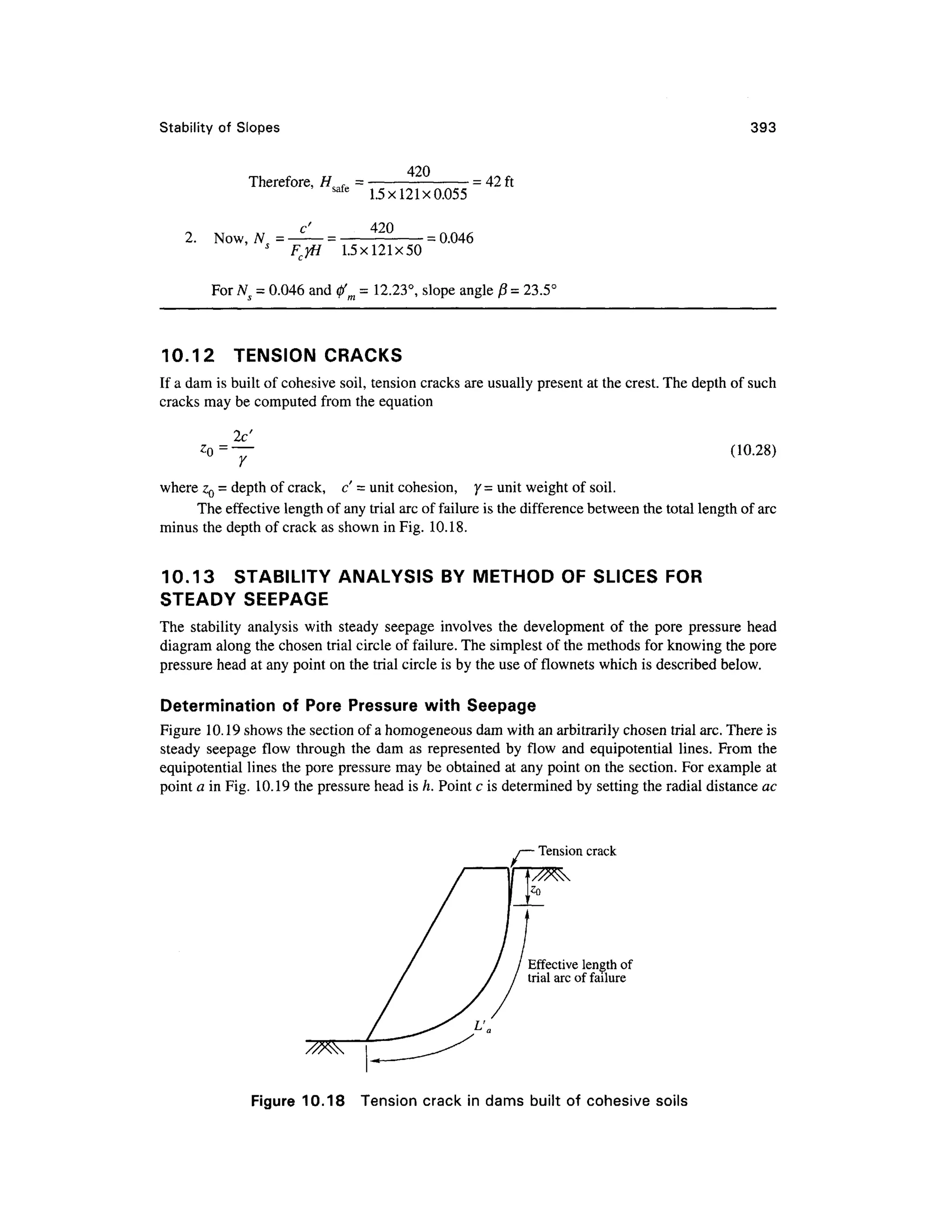
415. 396 Chapte r 1 0
The forces that are actually considered in the analysis are shown in Fig. 10.20(c) . The various
components ma y be determined as follows:
1 .Th e weight, W, of a slice per unit length of dam may be computed fro m
W=yhb
where, y = total unit weight of soil, h = average height of slice, b - widt h of slice.
If the widths of all slices are equal, and if the whole mass is homogeneous, th e weight W
can be plotted as a vector AB passing throug h the center of a slice as in Fig. 10.20(a) . AB
may be made equal to the height of the slice.
2. B y constructing triangle ABC, th e weight can be resolved int o a normal component N and
a tangential component T. Similar triangles can be constructed for all slices. The tangential
components of the weights cause the mass to slide downward. The sum of all the weight s
cause th e mass _ to slid e downward . The su m o f al l th e tangentia l component s ma y b e
expressed a s T= I.T. If the trial surface is curved upward near its lower end, the tangential
component of the weight of the slice will act in the opposite direction along the curve. The
algebraic su m of T should be considered.
3. Th e average pore pressure u acting on the base of any slice of length / may be found from
the pore pressure diagram shown in Fig. 10.20(b). The total pore pressure, U, on the base of
any slice is
U=ul
4. Th e effective normal pressure N' acting on the base of any slice is
N'=N- t/[Fig . 10.20(c)]
5. Th e frictional force Ff
actin g on the base of any slice resisting the tendency of the slice to
move downward is
F = (N - U ) tan 0'
where 0' is the effectiv e angl e o f friction. Similarl y th e cohesive forc e C " opposing th e
movement of the slice and acting at the base of the slice is
where c i s the effective unit cohesion. The total resisting force S acting on the base of the
slice is
S = C + F'= c'l + (N - U ) tan 0'
Figure 10.20(c ) shows the resisting forces actin g on the base of a slice.
The sum of all the resisting forces actin g on the base of each slice may be expressed a s
Ss = c'I,l+ tan 0' I(W- £/) = c'L + tan 0' X(N - U )
where £/ = L = length of the curved surface.
The moment s o f th e actuatin g an d resistin g force s abou t th e poin t o f rotatio n ma y b e
written as follows:
Actuating moment = R~LT
Resisting moment = R[c'L + tan 0' £(jV - U)]
The factor of safety F? may now be written as
(10.29)

416. Stability of Slope s 397
The variou s components shown in Eq. (10.29 ) can easily be represented graphicall y as
shown in Fig. 10.20(d) . The line AB represents to a suitable scale Z,(N - U) . BC is drawn
normal to AB at B and equal to c'L + tan 0' Z(N - U) . The line AD drawn at an angle 0'to
AB gives the intercept BD on BC equal to tan 0'Z(N- U). The length BE on BC is equal to
IT. Now
F =
BC
BE
(10.30)
Centers for Tria l Circle s Through Toe
The factor of safety Fs a s computed and represented by Eq. (10.29) applies to one trial circle. This
procedure is followed for a number of trial circles until one finds the one for which the factor of safety
is the lowest. This circle that gives the least Fs is the one most likely to fail. The procedure is quite
laborious. The number of trial circles may be minimized if one follows the following method.
For any given slope angle /3 (Fig. 10.21) , the center of the first tria l circle center O may be
determined as proposed by Fellenius (1927). The direction angles aA and aB may be taken fro m
Table 10.1. For the centers of additional trial circles, the procedure is as follows:
Mark point C whose position is as shown in Fig. 10.21 . Join CO. The centers of additional
circles lie on the line CO extended. This method is applicable for a homogeneous (c -</> ) soil. When
the soil is purely cohesive and homogeneous the direction angles given in Table 10.1 directly give
the center for the critical circle.
Centers for Tria l Circle s Belo w To e
Theoretically if the materials of the dam and foundation are entirely homogeneous, any practicable
earth dam slope may have its critical failure surface below the toe of the slope. Fellenius found that
the angle intersected at 0 in Fig. 10.22 for this case is about 133.5°. To find the center for the critical
circle below the toe, the following procedure is suggested.
Locus of centers
of critical circles
Curve of factor
of safet y
Figure 10.2 1 Locatio n of centers of critical circle passing through toe of dam

417. 398 Chapter 1 0
Figure 10.2 2 Center s o f tria l circles for bas e failur e
Table 10. 1 Directio n angle s a°A an d a°ofor center s o f critica l circle s
Slope Slope angl e Direction angles
0.6: 1
1 : 1
1.5: 1
2: 1
3: 1
5 : 1
60
45
33.8
26.6
18.3
11.3
29
28
26
25
25
25
40
37
35
35
35
37
Erect a vertical at the midpoint M of the slope. On this vertical will be the center O of the first
trial circle. In locating the trial circle use an angle (133.5°) between the two radii at which the circle
intersects th e surfac e of the embankment and the foundation. After the firs t tria l circle has bee n
analyzed the center is some what moved to the left, the radius shortened and a new trial circle drawn
and analyzed. Additional centers for the circles are spotted and analyzed.
Example 10.1 1
An embankment is to be made of a sandy clay having a cohesion o f 30 kN/m2
, angle of internal
friction o f 20° and a unit weight of 1 8 kN/m3
. The slope and height of the embankment are 1. 6 : 1
and 10m respectively. Determine the factor of safety by using the trial circle given in Fig. Ex. 10.11
by the method of slices.
Solution
Consider the embankment as shown in Fig. Ex.10.11. The center of the trial circle O is selected by
taking aA = 26° and aB = 35° from Table 10.1 . The soil mass above the slip circle is divided into 13
slices of 2 m width each. The weight of each slice per unit length of embankment is given by W =
haby;, where h a = average height of the slice, b = width of the slice, y t = unit weight of the soil.
The weigh t of each slic e may be represented by a vector of height ha if b and y, remain the
same for the whole embankment. The vectors values were obtained graphically. The height vectors

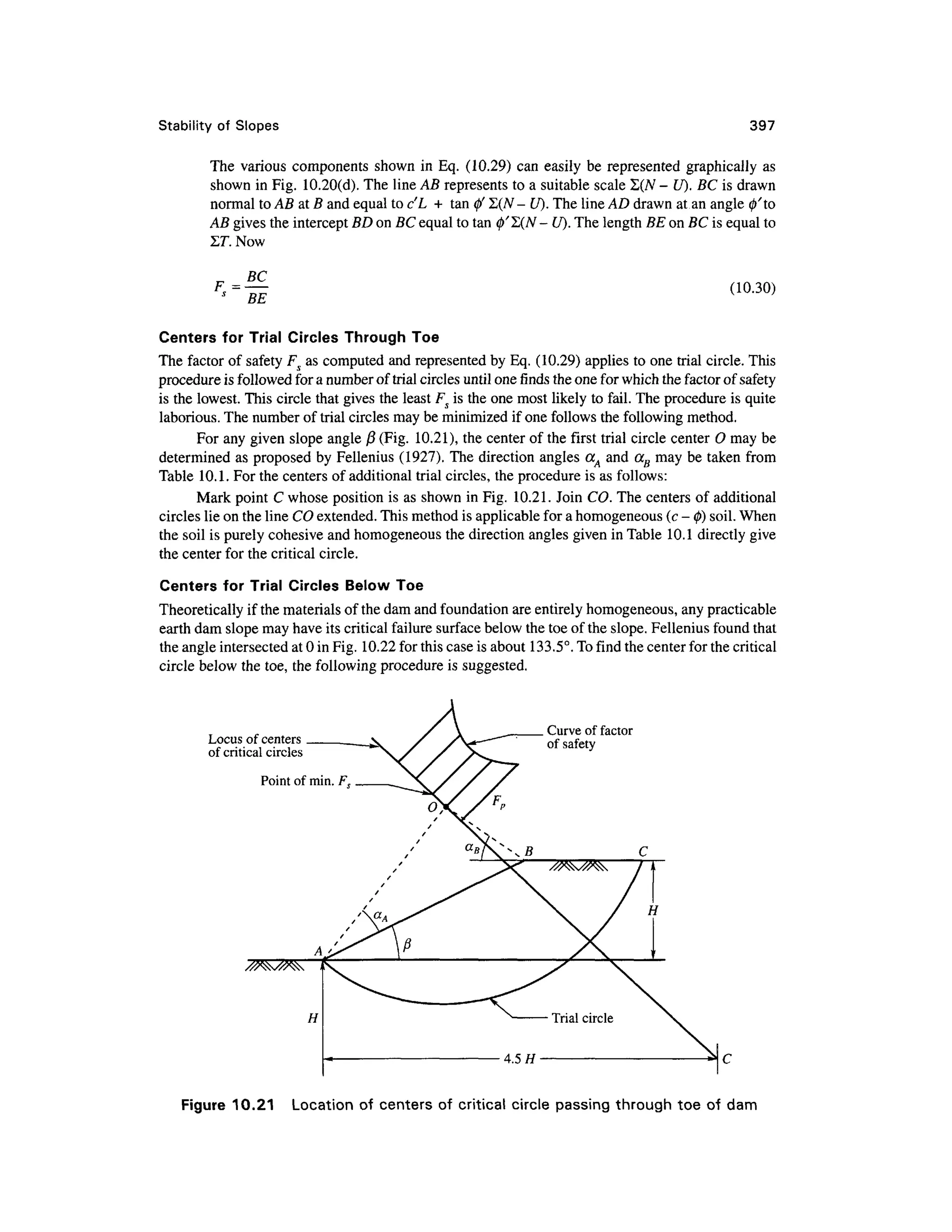
418. Stability of Slope s 399
Figure Ex. 10.11
may be resolved into normal components hn and tangential components h{. The values of ha, hn and
ht for the various slices are given below in a tabular form.
Values o f hal h n and /?,
o / v r
Slice No .
1
2
3
4
5
6
7
ha(m)
1.8
5.5
7.8
9.5
10.6
11.0
10.2
hn(m)
0.80
3.21
5.75
7.82
9.62
10.43
10.20
ht(m]
1.72
4.50
5.30
5.50
4.82
3.72
2.31
Slice No .
8
9
10
11
12
13
ha(m)
9.3
8.2
6.8
5.2
3.3
1.1
hn(m)
9.25
8.20
6.82
5.26
3.21
1.0
ht(m)
1.00
-0.20
-0.80
-1.30
-1.20
-0.50
The sum of these components hn and ht may be converted into forces ZN and Irrespectively
by multiplying them as given below
Sfcn = 81.57m, Ui t = 24.87m
Therefore, ZN = 81.57 x2 x 1 8 = 2937 kN
Zr = 24.87 x2x 1 8 =895kN
Length of arc = L = 31.8 m
'L + tonfiZ N 30x31. 8 + 0.364x2937
Factor of safety =
895
= 2.2
6

419. 400
10.14 BISHOP' S SIMPLIFIE D METHO D OF SLICES
Chapter 1 0
Bishop's metho d of slices (1955) is useful i f a slope consists of several types of soil with differen t
values of c and 0 and if the pore pressures u in the slope are known or can be estimated. The method
of analysis is as follows:
Figure 10.2 3 gives a section of an earth dam having a sloping surface AB. ADC is an assumed
trial circular failure surface with its center at O. The soil mass above the failure surface is divided
into a number of slices. The forces acting on each slice are evaluated from limit equilibrium of the
slices. The equilibrium of the entire mass is determined by summation of the forces on each of the
slices.
Consider fo r analysis a single slice abed (Fig . 10.23a ) which is drawn to a larger scal e in
Fig. 10.23(b) . The forces acting on this slice are
W = weight of the slice
N = total normal forc e on the failure surface cd
U = pore water pressure = ul on the failure surface cd
FR = shear resistance acting on the base of the slice
Er E2 - norma l forces on the vertical faces be and a
d
Tr T 2 = shear forces on the vertical faces be and ad
6 = the inclination of the failure surface cd to the horizontal
The syste m i s staticall y indeterminate . A n approximat e solutio n ma y b e obtaine d b y
assuming tha t the resultan t of £, an d T^ i s equal t o that of E 2 an d T 2, and thei r line s o f actio n
coincide. Fo r equilibrium of the system, the following equations hold true.
O
(a) (b )
Figure 10.2 3 Bishop' s simplified method of analysi s

420. Stability o f Slope s 40 1
N=Wcos6
(10.31)
where F( = tangentia l component of W
The unit stresses on the failure surface of length, /, may be expressed a s
Wcos6
normal stress, <r n = -
Wsin0 (10.32 )
shear stress, r n = -
The equation for shear strength, s, is
s = c' + cr'tan^' = c' + (cr-u)tan0'
where r f = effective normal stress
c' - effectiv e cohesio n
(ft = effective angle of friction
u = unit pore pressur e
The shearing resistance to sliding on the base of the slice is
si = c'l+ (Wcos9 -ul) tan $
where ul = U, the total pore pressure on the base of the slice (Fig 10.23b )
d = F
At - r R
The total resisting force and the actuating force on the failure surface ADC may be expressed
as
Total resisting force FR is
FR= [c 7 + (Wcos0-M/)tan0'] (10.33 )
Total actuating force Ft is
Ft = Wsm0 (10.34 )
The factor of safety Fs is then given as
F
Eq. (10.35) is the same as Eq. (10.29) obtained b y the conventional metho d of analysis .
Bishop (1955) suggest s tha t the accuracy of the analysis can be improved b y taking into
account the forces E and Ton the vertical faces of each slice. For the element in Fig. 10.23(b) , we
may writ e a n expressio n fo r al l th e force s actin g in th e vertica l directio n fo r th e equilibrium
condition as
N' co&0 = W + (T^ -T2)-ulcos0- F R sin# (10.36 )
If th e slop e i s no t o n th e verg e of failur e (Fs > 1), the tangentia l force F t i s equal t o th e
shearing resistance FR on cd divided by Fg.

421. 402 Chapter 1 0
c'l
(10.37)
where, N'=N-U,andU= ul.
Substituting Eq. (10.37) into Eq. (10.36) and solving for N we obtain
c'l
— sin< 9
F
cos<9 +
tan 0' sin 6
F..
(10.38)
where, AT= T{ - Tr
For equilibrium of the mass above the failure surface, we have by taking moments about O
Wsin0R = F RR (10.39 )
By substituting Eqs. (10.37) and (10.38) into Eq. (10.39) and solving we obtain an expression
forF a s
F
where,
tan(/>' sin 9
F
(10.40)
(10.41)
The factor of safety FS i s present in Eq. (10.40) on both sides. The quantity AT=T{ - T 2 has
to be evaluated by means of successive approximation . Trial value s of E^ an d T l tha t satisfy the
equilibrium of each slice, and the conditions
1.6
1.4
1.2
1.0
mf) = cos 6 + (sin 6tan d) )/F
i i i
Note: 0 is + when slope of failure
arc is in the same quadrant
as ground slope.
0.6
-40 -3 0 -2 0 -1 0 0 1 0 2 0
Values of 6 degrees
30 40
Figure 10.2 4 Value s of mfi (afte r Janbu et al., 1956 )

422. Stability of Slope s 403
(El-E2) = Q an d (r l-T2) = 0
are used. The value of Fs ma y then be computed by first assumin g an arbitrary value for Fs. The
value of Fs may then be calculated by making use of Eq. (10.40). If the calculated value of Fv differs
appreciably fro m th e assume d value , a secon d tria l i s mad e an d th e computatio n i s repeated .
Figure 10.24 developed by Janbu et al. (1956) helps to simplify th e computation procedure.
It is reported that an error of about 1 percent will occur if we assume Z(Tj - T" 2) tan0'= 0. But
if w e us e th e conventiona l method o f analysi s using Eq. (10.35 ) th e erro r introduce d i s abou t
15 percent (Bishop, 1955) .
10.15 BISHO P AND MORGENSTER N METHO D FOR SLOPE ANALYSIS
Equation (10.40) develope d base d on Bishop's analysi s of slopes, contains the term pore pressure
u. The Bishop and Morgenstern method (1960) proposes the following equation for the evaluation
of u
yh (10.42)
where, u = pore water pressure at any point on the assumed failure surface
Y= unit weight of the soil
h = the depth of the point in the soil mass below the ground surface
The pore pressure ratio ru is assumed to be constant throughout the cross-section, which is
called a homogeneous pore pressure distribution. Figur e 10.25 shows the various parameters use d
in the analysis.
The factor of safety F i s defined as
F_ = m - nr,. (10.43)
where, m, n = stability coefficients.
The m and n values may be obtained either from charts in Figs. B. 1to B.6 or Tables B1 to B6
in Appendix B. The depth factor given in the charts or tables is as per Eq. (10.25), that is nd = DIH,
where H = height of slope, an d D = depth of firm stratu m from th e top of the slope. Bishop and
Morgenstern (1960 ) limited their charts (o r tables) to values of c'ly H equal to 0.000, 0.025, and
0.050.
Center of failure surface
Failure surfac e
y = unit weight of soil
/^^^^^^^^//^f^^^
Figure 10.2 5 Specification s o f parameter s for Bishop-Morgenster n metho d of
analysis

423. 404 Chapter 1 0
Extension o f th e Bisho p an d Morgenster n Slop e Stabilit y Chart s
As stated earlier, Bisho p and Morgenstern (1960) charts o r tables cove r value s of c'lyH equa l t o
0.000, 0.025, and 0.050 only. These charts do not cover the values that are normally encountered in
natural slopes. O' Connor an d Mitchell (1977 ) extende d th e work of Bishop an d Morgenstern t o
cover values of c'lyH equa l to 0.075 an d 0.100 for various values of depth factors nd. The method
employed i s essentially th e same a s that adopted b y the earlier authors . The extended value s are
given in the form of charts and tables from Figs. B.7 to B.14 and Tables B7 to B14 respectively in
Appendix B.
Method o f Determinin g F s
1. Obtai n the values of ru and clyH
2. Fro m the tables in Appendix B, obtain the values of m and n for the known values ofc/yH,
0 and /3, and for nd - 0 , 1, 1.2 5 and 1.5.
3. Usin g Eq. (10.43), determine Fs for each value of nd.
4. Th e required value of Fs is the lowest of the values obtained in step 3.
Example 10.1 2
Figure Ex. 10.1 2 gives a typical section o f a homogeneous earth dam . The soi l parameters are:
0' = 30°, c' = 590 lb/ft2
, an d y = 120 lb/ft3
. Th e da m has a slope 4: 1 and a pore pressur e rati o
ru = 0.5. Estimate the factor of safety Fs b y Bishop and Morgenstern method for a height of dam
#=140 ft.
Solution
Height of dam H= 140f t
c' 59 0
120x140
= 0.035
Given: 0' = 30°, slope 4:1 and ru = 0.5.
Since c'lyH = 0.035, an d nd = 1.43 for H = 140 ft, the Fs fo r th e dam lie s between c'lyH
0.025 an d 0.05 and nd between 1. 0 and 1.5. The equation for Fs is
= m-nr
Using the Tables in Appendix B, the following table can be prepared for the given values of
c'lyH, 0 , and /3.
0'=30°
c' = 590psf
y - 12 0 pcf
/•„ = 0.5 0
D = 200 ft
Alluvium (same properties a s above)
Figure Ex. 10.12

424. Stability o f Slopes 40 5
From Tables B 2 and B3 for c'/yH = 0.02 5
n
d
1.0
1.25
From Table B4, B5
n
d
1.0
1.25
1.50
m
2.873
2.953
and B6 for c'ljH - 0.0 5
m
3.261
3.221
3.443
n
2.622
2.806
n
2.693
2.819
3.120
F,
1.562
1.55
F,
1.915
1.812
1.883
Lowest
Lowest
Hence n d = 1.2 5 i s the mor e critica l dept h factor . The valu e of F s fo r c'lyH = 0.035 lie s
between 1.5 5 (for c'lyH = 0.025) and 1.81 2 (for c'lyH = 0.05). By proportion F = 1.655.
10.16 MORGENSTER N METHO D O F ANALYSIS FO R RAPID
DRAWDOWN CONDITIO N
Rapid drawdown of reservoir wate r level is one of the critical state s in the design of earth dams.
Morgenstern (1963) developed the method of analysis for rapid drawdown conditions based on the
Bishop and Morgenstern method of slices. The purpose of this method is to compute the factor of
safety durin g rapid drawdown, which is reduced under no dissipation of pore water pressure. The
assumptions made in the analysis are
1. Simpl e slope of homogeneous materia l
2. Th e dam rests on an impermeable bas e
3. Th e slope is completely submerge d initially
4. Th e pore pressure doe s not dissipate during drawdown
Morgenstern use d the pore pressure parameter 5 a s developed b y Skempton (1954) whic h
states
5 = — (10.45 )
where cr , = y h
j- total unit weight of soil or equal to twice the unit weight of water
h = height of soil above the lower level of water after drawdown
The charts developed tak e into account the drawdown ratio which is defined as
(10.46)
where Rd = drawdown ratio
// = height of drawdown
H = height of dam (Fig. 10.26 )
All the potential sliding circles must be tangent to the base of the section.

425. 406 Chapter 1 0
Full reservoir level
" Drawdow n
/level H
Figure 10.2 6 Da m section for drawdow n condition s
The stability charts are given in Figs. 10.2 7 to 10.2 9 coverin g a range of stability numbers
c'/yH fro m 0.0125 to 0.050. The curves developed are for the values of 0'of 20°, 30°, and 40° for
different value s of B.
PL,
0.2 0. 4 0. 6 _0. 8
Drawdown ratio H/H
(a) 0 = 2:1
1.0 0 0. 2 0. 4 0. 6 _0. 8
Drawdown ratio H/H
<P
40°
30°
20°
0.2 0. 4 0. 6 _0. 8
Drawdown ratio H/H
1.0
Figure 10.2 7
0.2 0. 4 0. 6 _0. 8 1. 0
Drawdown ratio H/H
(d) ft = 5:1
Drawdown stabilit y char t for c'/yH = 0.012 5 (afte r Morgenstern ,
1963)

426. Stability of Slope s 407
40°
30°
20°
0.2 0. 4 0. 6 _0. 8 1. 0
Drawdown ratio H/H
(a) ft = 2:1
40°
30°
20°
0 0. 2 0. 4 0. 6 _0. 8 1. 0
Drawdown ratio H/H
(b) ft = 3:1
0.2 0. 4 0. 6 _0. 8
Drawdown ratio H/H
(c) ft = 4:1
<P
40°
30°
20°
1.0
i*,
>*
UH
(d) 0=5:
<P
40°
30°
20°
0 0. 2 0. 4 0. 6 _0. 8 1. 0
Drawdown ratio H/H
Figure 10.2 8 Drawdow n stabilit y chart fo r c'lyH = 0.02 5 (afte r Morgenstern ,
1963)
Example 10.1 3
It is required to estimate th e minimum factor of safety for the complete drawdow n of the sectio n
shown in Fig. Ex. 10.1 3 (Morgenstern, 1963 )
.*._./:
Water level befor e
drawdown
Water level afte r
drawdown
Figure Ex. 10.13

427. 408 Chapter 1 0
Solution
From the data given in the Fig. Ex . 10.1 3
N = —=
312
= 0.025
yH. 124.8x10 0
From Fig . 10.28 , fo r W = 0.025, 0=3:1,</> ' = 30°, an d H/ H = 1,
Fs = 1.20
It is evident than the critical circle is tangent to the base of the dam and no other level need be
investigated sinc e thi s woul d onl y rais e th e effectiv e valu e o f N S resultin g i n a higher facto r o f
safety.
10.17 SPENCE R METHO D O F ANALYSI S
Spencer (1967 ) develope d hi s analysi s base d o n th e metho d o f slice s o f Felleniu s (1927 ) an d
Bishop (1955) . Th e analysi s i s i n term s o f effectiv e stres s an d satisfie s tw o equation s o f
X
0.2 0. 4 0. 6 _0. 8
Drawdown ratio H/H
0 0.2 0. 4 0. 6 _0. 8
Drawdown ratio H/H
40°
30°
20°
1.0 0.2 0. 4 0. 6 _0. 8
Drawdown ratio H/H
n- 2
k
.
l
X
X
X
X
X
x
.^"•^
X
x^
»^_
—
——E^M
40°
30°
20°
0 0.2 0. 4 0. 6 _0. 8
Drawdown ratio H/H
1.0
(c) ft = 4:1 (d) ft = 5:1
Figure 10.2 9 Drawdow n stability chart for c'lyH = 0.0 5 (afte r Morgenstern , 1963 )

428. Stability o f Slope s 40 9
equilibrium, the first with respect to forces and the second with respect to moments. The interslice
forces are assumed to be parallel a s in Fig. 10.23 . The factor of safety Ff i s expressed a s
Shear strength available
F = CI O 47)
5
Shea r strength mobilized ' '
The mobilized angle of shear resistance and other factors are expressed as
(10.48)
u
pore pressure ratio, r = — n n 49)
yh^ ' '
c'
Stability factor, N S= —— (10.50 )
The charts developed by Spencer for different values of Ns, §'m and ru are given in Fig. 10.30.
The use of these charts will be explained with worked out examples.
Example 10.1 4
Find the slope corresponding t o a factor of safety of 1. 5 for an embankment 10 0 ft high in a soil
whose properties ar e as follows:
c' = 870 Ib/sq ft, y= 120 Ib/ft3,</> ' = 26°, ru = 0.5
Solution (b y Spencer's Method )
N = ^L= 87 0
5
F sytl 1.5x120x10 0
t ., tan f 0.48 8 _ „ _
tan 0 = -
—= -
=0.325
F 1. 5
Referring to Fig. 10.30c , for which r = 0.5 , the slope corresponding t o a stability number
of 0.048 is 3:1.
Example 10.1 5
What would be the change in strength on sudden drawdown for a soil element at point P which is
shown i n Fig. Ex . 10.15 ? Th e equipotential line passing throug h this element represent s los s of
water head of 1.2 m. The saturated unit weight of the fill is 21 kN/m3
.
Solution
The data given are shown in Fig. Ex. 10.15. Before drawdown,
The stresses at point P are:
% = /
A +
nA = 9.81 x 3 + 21 x4 =113 kN/m2
"o = Yw (hw + h
c- h'} = 9.81(3 + 4 - 1.2 ) = 57 kN/m2

429. 410 Chapter 1 0
4:1 3: 1 2:1
0.12
0.10
0.08
?L
^0.06
j
0.04
0.02
4:1 3: 1 2:1 1.5:
2 4 6 8 1 0 1 2 1 4 1 6 1 8 2 0 2 2 2 4 2 6 2 8 3 0 3 2 3 4
Slope angle/?, degrees
Figure 10.3 0 Stabilit y chart s (afte r Spencer, 1967 )

430. Stability of Slopes 411
Figure Ex. 10.15
Therefore tf 0 = (JQ - U Q = 113 - 5 7 =56 kN/m2
After drawdown,
o= ysathc = 21 x 4 = 84 kN/m2
u = yw (hc - h'} = 9.81(4 - 1.2 ) = 27.5 kN/m2
of
= a-u= S4-27.5 = 56.5 kN/m2
The change in strength is zero since the effective vertica l stress does not change.
Note: There is no change in strength due to sudden drawdown but the direction of forces of
the seepage water changes from an inward direction before drawdown to an outward direction afte r
drawdown and this is the main cause for the reduction in stability.
10.18 PROBLEM S
10.1 Fin d the critical height of an infinite slope having a slope angle of 30°. The slope is made of
stiff cla y having a cohesion 2 0 kN/m2
, angle of internal friction 20° , voi d ratio 0.7 and
specific gravity 2.7. Consider the following cases for the analysis.
(a) the soil is dry.
(b) the water seeps parallel to the surface of the slope.
(c) the slope is submerged.
10.2 A n infinite slope ha s a n inclination of 26° with the horizontal. I t is underlain by a firm
cohesive soi l havin g Gs = 2.72 and e = 0.52. Ther e i s a thin weak layer 20 ft below and
parallel to the slope (c' - 52 5 lb/ft2
, 0' = 16°). Compute the factors of safety when (a) the
slope is dry, and (b) ground water flows parallel to the slope at the slope level.
10.3 A n infinite slope is underlain with an overconsolidated clay having c' - 21 0 lb/ft2
, 0' = 8°
and ysat = 12 0 lb/ft3
. The slope is inclined at an angle of 10 ° to the horizontal. Seepage is
parallel t o the surface and the ground water coincides wit h the surface. If the slope fail s
parallel to the surface along a plane at a depth of 12 ft below the slope, determine the factor
of safety.
10.4 A deep cut of 1 0 m depth is made in sandy clay for a road. The sides o f the cut make an
angle o f 60 ° wit h th e horizontal . Th e shea r strengt h parameter s o f th e soi l ar e
c' - 2 0 kN/m2
, fi = 25°, and 7= 18. 5 kN/m3
. If AC is the failure plane (Fig Prob. 10.4) ,
estimate the factor of safety of the slope.

431. 412 Chapter 1 0
y= 18.5kN/m 3
Figure Prob . 10. 4
W = 1050 kN
Figure Prob. 10. 5
10.5 A 40° slope is excavated to a depth of 8 m in a deep layer of saturated clay having strength
parameters c = 60 kN/m2
, 0 = 0, and y= 19 kN/m3
. Determine the factor of safety for the
trial failure surface shown in Fig. Prob. 10.5 .
10.6 A n excavation to a depth of 8 m with a slope of 1: 1 was made in a deep layer of saturated
clay having cu = 65 kN/m2
and 0 M = 0. Determine the factor of safety for a trial slip circle
passing through the toe of the cut and having a center as shown in Fig. Prob. 10.6 . The unit
weight of the saturated clay is 1 9 kN/m3
. No tension crack correction i s required.
10.7 A 45° cu t was made in a clayey silt with c = 15 kN/m2
, 0 =0 and y = 19. 5 kN/m 3
. Sit e
exploration revealed th e presence o f a soft cla y stratum of 2 m thick having c = 25 kN/m2
and 0 = 0 as shown in Fig. Prob . 10.7 . Estimat e th e factor of safety o f the slop e fo r the
assumed failure surface .
10.8 A cut was made in a homogeneous clay soil to a depth of 8 m as shown in Fig. Prob. 10.8 . The
total uni t weigh t o f th e soi l i s 1 8 kN/m 3
, an d it s cohesiv e strengt h i s 2 5 kN/m 2
.

432. Stability of Slope s 413
<§)
Figure Prob. 10. 6
Figure Prob. 10. 7
Assuming a 0 =0 condition, determine the factor of safety with respect to a slip circle passing
through the toe. Consider a tension crack at the end of the slip circle on the top of the cut.
10.9 A deep cut of 1 0 m depth is made in natural soil for the construction o f a road. The soil
parameters are : c' = 35 kN/m2
, 0' = 15° and 7= 2 0 kN/m3
.
Figure Prob. 10. 8

433. 414 Chapter 1 0
Figure Prob . 10. 9
The sides of the cut make angles of 45° with the horizontal. Compute the factor of safet y
using friction circle method for the failure surface AC shown in Fig. Prob. 10.9 .
10.10 A n embankment is to be built to a height of 50 ft at an angle of 20° with the horizontal. The
soil parameters are: c' - 63 0 lb/ft2
, 0' = 18° and 7= 11 5 lb/ft3
.
Estimate the following;
1. Facto r of safety of the slope assuming full frictio n i s mobilized.
2. Facto r of safety with respect to friction if the factor of safety with respect to cohesion is
1.5.
Use Taylor's stability chart.
10.11 A cut was made in natural soil for the construction of a railway line. The soil parameter s
are: c' = 700 lb/ft2
, 0' = 20° and 7= 11 0 lb/ft3
.
Determine the critical height of the cut for a slope of 30° with the horizontal by making use
of Taylor's stability chart.
10.12 A n embankment i s to be constructed b y making us e of sandy cla y havin g the following
properties: c' = 35 kN/m2
, 0' = 25° and y= 19.5 kN/m3
.
The height of the embankment is 20 m with a slope of 30° with the horizontal as shown in
Fig. Prob . 10.12 . Estimate the factor of safety by the method o f slices fo r the trial circl e
shown in the figure.
10.13 I f an embankment of 10 m height is to be made from a soil having c' = 25 kN/m2
, 0' = 15°,
and 7=18 kN/m3
, what will be the safe angle of slope for a factor of safety of 1.5 ?
10.14 A n embarkmen t i s constructe d fo r a n eart h da m o f 8 0 f t hig h a t a slop e o f 3:1 . Th e
properties o f th e soi l use d fo r th e constructio n are : c - 77 0 lb/ft 2
, 0 ' = 30° , an d
7=110 lb/ft3
. The estimated pore pressuer ratio r = 0.5 . Determine the factor of safety by
Bishop and Morgenstern method.
10.15 Fo r the Prob. 10.14 , estimate the factor of safety for 0' =20°. All the other data remain the
same.
10.16 Fo r the Prob. 10.14 , estimate the factor of safety for a slope of 2:1 with all the oother data
remain the same.

434. Stability o f Slope s 415
Figure Prob. 10.12
10.17 A cu t o f 2 5 m dopt h i s mad e i n a compacted fil l havin g shea r strengt h parameter s o f
c = 25 kN/m2
, and 0' = 20°. The total unit weight of the material is 1 9 kN/m3
. The por e
pressuer ratio has an average value of 0.3. The slope of the sides is 3:1. Estimate the factor
of safety using the Bishop and Morgenstern method.
10.18 Fo r the Prob. 10.17 , estimate the factor of safety for 0'= 30°, with all the other data remain
the same.
10.19 Fo r the Prob. 10.17 , esatimate the factor of safety for a slope of 2:1 with all the other data
remaining the same.
10.20 Estimat e the minimum factor of safety for a complete drawdown condition for the section
of dam in Fig. Prob. 10.20 . The full reservoir level of 1 5 m depth is reduced t o zero after
drawdown.
10.21 Wha t is the safety factor if the reservoir level is brought down from 15 m to 5 m depth in
the Prob. 10.20 ?
10.22 A n earth dam to be constructed at a site has the following soil parameters: c' = 60 0 lb/ft2
,
y =110 lb/ft3
, an d 0' =20°. The height of of dam H = 50 ft.
The pore pressure ratio ru = 0.5. Determine the slope of the dam for a factor of safety of 1.5
using Spencer's method (1967) .
c' = 15 kN/m2
<f>' = 30 °
y = 20 kN/m3
Figure Prob. 10.2 0

435. 416 Chapter 1 0
O
R = 45 ft
15ft
Figure Prob . 10.2 4
10.23 I f the given pore pressure rati o is 0.25 i n Prob. 10.22 , what will be the slope o f the dam?
10.24 A n embankment has a slope of 1.5 horizontal to 1 vertical with a height of 25 feet. The soil
parameters are :
c - 60 0 lb/ft2
, 0 ' = 20°, and 7=11 0 lb/ft3
.
Determine the factor of safety using friction circle method for the failure surface AC shown
in Fig. Prob. 10.24 .
10.25 I t is required to construct an embankment for a reservoir t o a height of 20 m at a slope of
2 horizontal to 1 vertical. The soil parameters are :
c = 40 kN/m2
, f = 18°, and 7= 17. 5 kN/m3
.
Estimate th e following:
1. Factor o f safety of the slope assuming full frictio n i s mobilized.
2. Factor o f safety wit h respect to friction i f the factor of safety with respect to cohesion i s
1.5.
Use Taylor's stabilit y chart.
10.26 A cutting o f 40 ft depth i s to be mad e fo r a road a s shown i n Fig. Prob . 10.26 . The soi l
properties are :
c' = 500 lb/ft2
, 0 ' = 15° , and 7= 11 5 lb/ft 3
.
Estimate the factor of safety by the method of slices for the trial circle shown in the figure.
10.27 A n eart h da m i s t o b e constructe d fo r a reservior . Th e heigh t o f th e da m i s 6 0 ft . Th e
properties of the soil used in the construction are:
c = 400 lb/ft2
, 0 ° =20°, and 7= 11 5 lb/ft3
, an d ft = 2:1.
Estimate the minimum factor of safety for the complete drawn from the full reservior leve l
as shown in Fig. Prob. 10.2 7 by Morgenstern method.
10.28 Wha t is the factor of safety i f the water level is brought down from 60 ft to 20 ft above th e
bed level of reservoir in Prob. 10.27 ?

436. Stability of Slopes 417
c' = 5001b/ft2
0'=15°
y=1151b/ft3
Figure Prob. 10.2 6
Full reservoir level
1
Figure Prob . 10.2 7
10.29 Fo r the dam given in Prob. 10.27, determine the factor of safety for r«=0.5 by Spencer' s
method.

438. CHAPTER 11
LATERAL EARTH PRESSURE
11.1 INTRODUCTIO N
Structures that are built to retain vertical or nearly vertical eart h bank s or any other material are
called retaining walls. Retaining walls may be constructed of masonry or sheet piles. Some of the
purposes for which retaining walls are used are shown in Fig. 11.1 .
Retaining wall s may retain wate r also. The eart h retained ma y be natural soil o r fill. Th e
principal types of retaining walls are given in Figs. 11. 1 and 11.2.
Whatever ma y b e th e typ e o f wall , al l th e wall s liste d abov e hav e t o withstan d latera l
pressures either from earth or any other material on their faces. The pressures acting on the walls try
to move the walls from thei r position. The walls should be so designed a s to keep them stable in
their position. Gravit y walls resist movemen t because o f their heavy sections . The y ar e built of
mass concrete or stone or brick masonry. No reinforcement is required in these walls. Semi-gravity
walls are not as heavy as gravity walls. A small amount of reinforcement is used for reducing the
mass of concrete. The stems of cantilever walls are thinner in section. The base slab is the cantilever
portion. These walls are made of reinforced concrete . Counterfor t walls are similar to cantilever
walls excep t tha t th e ste m o f th e wall s spa n horizontall y betwee n vertica l bracket s know n a s
counterforts. Th e counterfort s ar e provided o n the backfill side . Buttresse d wall s are similar t o
counterfort wall s except th e brackets o r buttress walls are provide d o n th e opposite sid e o f the
backfill.
In all these cases, the backfill tries to move the wall from its position. The movement of the
wall is partly resisted b y the wall itself an d partly by soil in front of the wall.
Sheet pile walls are more flexible than the other types. The earth pressure on these walls is
dealt wit h i n Chapte r 20 . Ther e i s anothe r typ e o f wal l tha t i s gainin g popularity . Thi s i s
mechanically stabilize d reinforce d eart h retaining walls (MSE) whic h will be dealt with later on.
This chapter deals with lateral earth pressures only.
419

439. 420 Chapter 1 1
(c) A bridge abutment (d) Water storage
.VI
(e) Flood walls (f) Sheet pile wall
Figure 11. 1 Us e of retainin g wall s
11.2 LATERA L EART
H PRESSURE THEOR
Y
There are two classical earth pressure theories. They are
1. Coulomb' s earth pressure theory.
2. Rankine' s earth pressure theory.
The firs t rigorou s analysi s of th e proble m o f latera l eart h pressur e wa s published
by Coulom b i n (1776) . Rankin e (1857 ) proposed a different approac h t o th e problem .
These theories propose to estimate the magnitudes of two pressures called active earth pressure
and passive earth pressure as explained below.
Consider a rigi d retainin g wall wit h a plan e vertica l face , a s show n i n Fig . 11.3(a), i s
backfilled wit h cohesionless soil . If the wall does no t move even after bac k filling , th e pressur e
exerted o n the wall is termed a s pressure for the at rest condition o f the wall. If suppose the wall
gradually rotates about point A and moves away from th e backfill, the unit pressure on the wall is
gradually reduced and after a particular displacement of the wall at the top, the pressure reaches a
constant value. The pressure is the minimum possible. This pressure is termed the active pressure
since the weight of the backfill is responsible for the movement of the wall. If the wall is smooth,

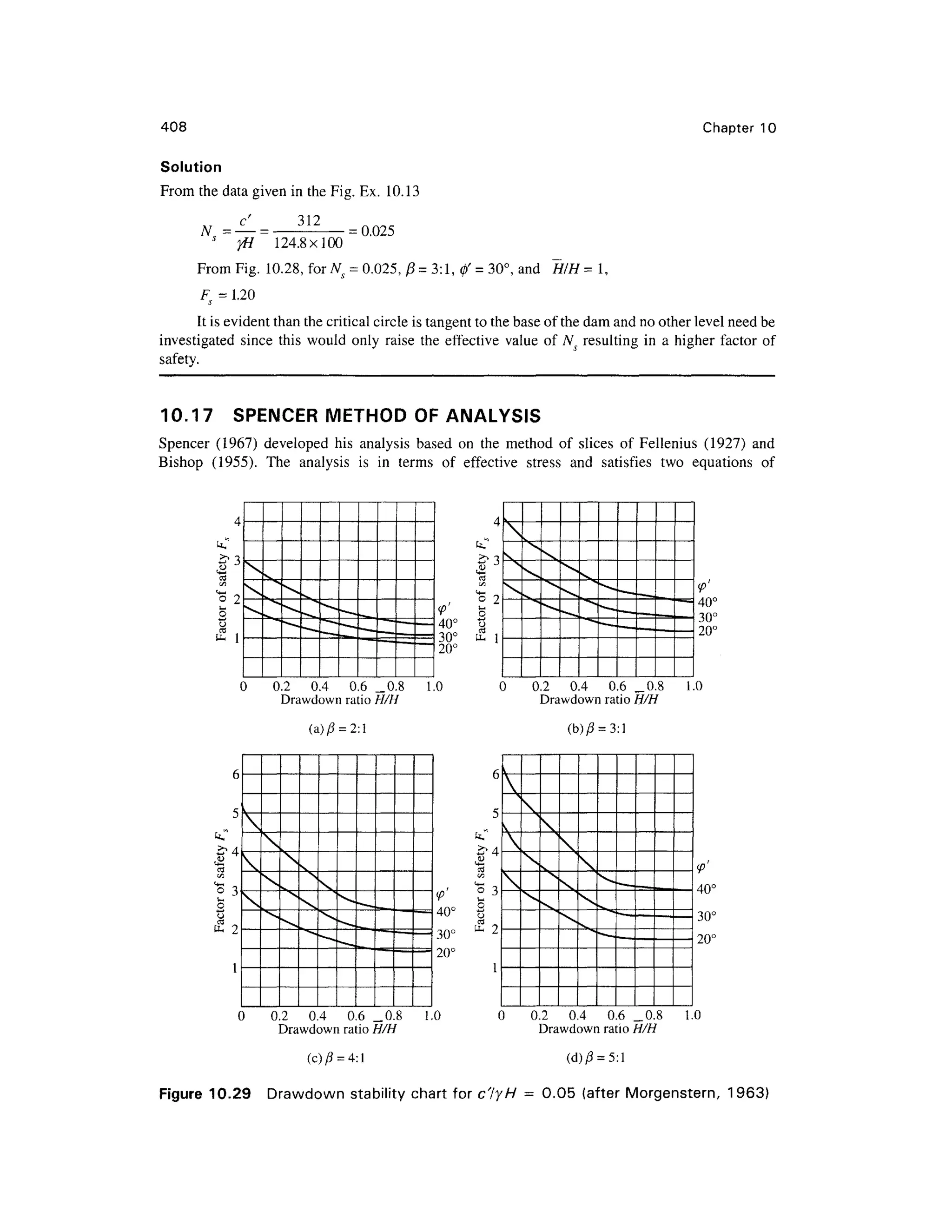
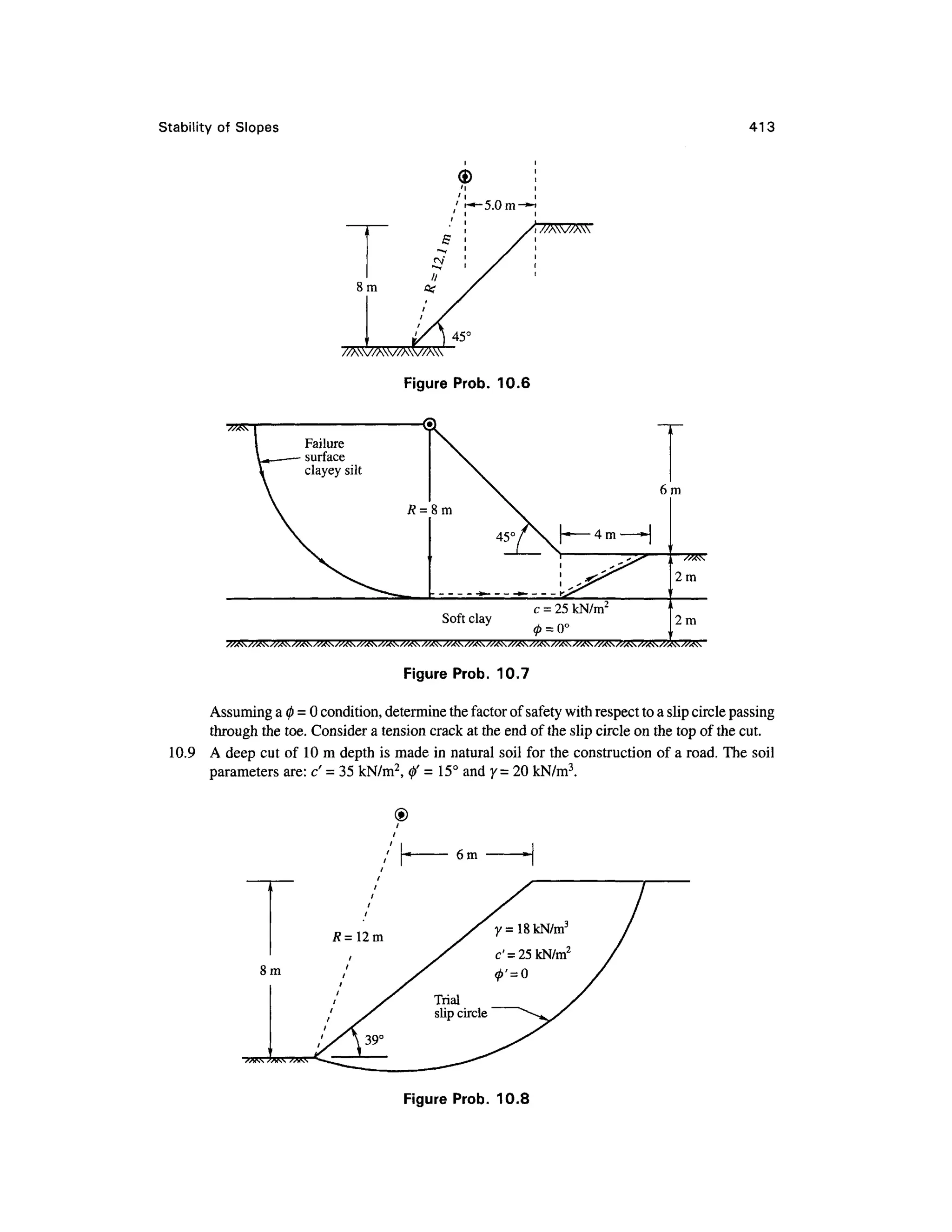
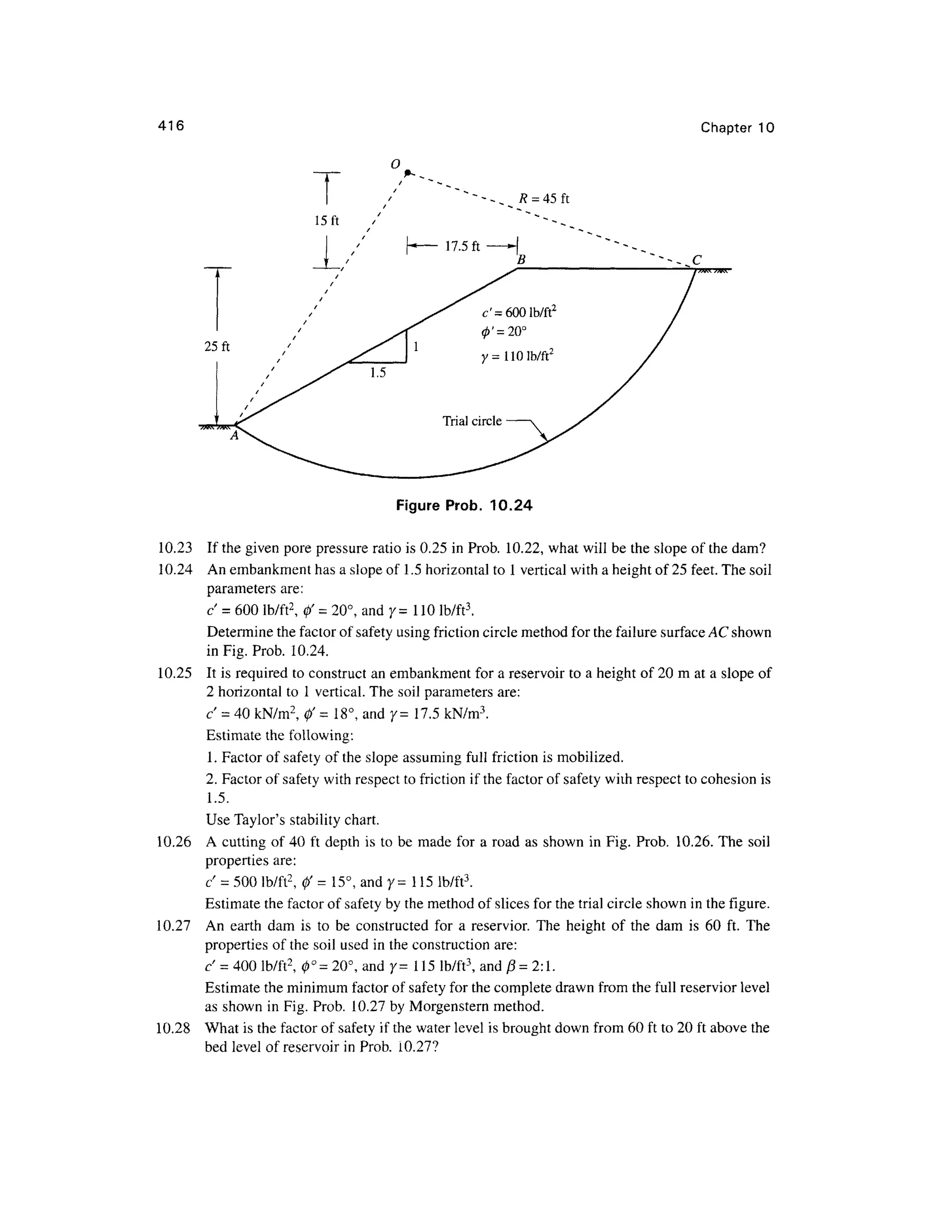
440. Lateral Eart h Pressure 421
Base sla b
Heel
(a) Gravity walls (b) Semi-gravity walls (c) Cantilever walls
Backfill Counterfort Fac e of wall —i
— Buttres s
Face
of wall
(d) Counterfort walls (e) Buttressed walls
Figure 11. 2 Principa l types of rigid retaining wall s
the resultant pressure acts normal to the face of the wall. If the wall is rough, it makes a n angle< 5
with the normal on the wall. The angle 8 is called the angle of wall friction.A s the wall moves away
from the backfill, the soil tends to move forward. When the wall movement is sufficient, a soil mass
of weight W ruptures along surface ADC shown in Fig. 11.3(a) . This surface is slightly curved. If
the surface is assumed to be a plane surface AC, analysis would indicate tha t this surface would
make an angle of 45° + 0/2 with the horizontal.
If the wall is now rotated about A towards the backfill, th e actual failure plane ADC is also a
curved surface [Fig. 11.3(b)]. However, if the failure surface is approximated as a plane AC, this
makes an angle 45° - 0/ 2 with the horizontal and the pressure on the wall increases from the value
of the at rest condition to the maximum value possible. The maximum pressure P tha t is developed
is terme d th e passive earth pressure. Th e pressure i s called passiv e becaus e th e weigh t o f the
backfill opposes the movement of the wall. It makes an angle 8 with the normal if the wall is rough.
The gradual decrease or increase of pressure on the wall with the movement of the wall from
the at rest condition may be depicted as shown in Fig. 11.4 .
The movement A require d to develop the passive state is considerably larger than AQ required
for the active state .
11.3 LATERA L EARTH PRESSURE FO R AT RES T CONDITION
If the wall is rigid and does not move with the pressure exerted on the wall, the soil behind the wall
will be in a state of elastic equilibrium. Consider a prismatic element E in the backfill at depth z
shown in Fig. 11.5 .
Element E is subjected to the following pressures.
Vertical pressure = crv= yz; latera l pressure = <J h

441. 422 Chapter 1 1
(a) Active earth pressure
(b) Passive earth pressure
Figure 11. 3 Wal l movemen t fo r the development o f activ e an d passive eart h
pressures
where yis the effective unit weight of the soil. If we consider the backfill is homogeneous then both
cry and oh increase linearly with depth z. In such a case, the ratio of ah to<J V remains constant with
respect to depth, that is
—- = —-= constant = AT ,
cr y z (11-1)
where KQ is called the coefficient o f earth pressure for th e at rest condition or at rest earth pressure
coefficient.
The lateral earth pressure oh acting on the wall at any depth z may be expressed a s
cr, - (11.la)

442. Lateral Earth Pressur e 423
Passive pressure
Away from backfil l Into backfil l
Figure 11.4 Developmen t o f active an d passive earth pressure s
H
z z
H/3
L
A
Ph = K
tiYZ
(a) (b )
Figure 11.5 Latera l earth pressur e for a t rest condition
The expression fo r oh at depth H, the height of the wall, is
The distribution of oh on the wall is given in Fig. 11.5(b) .
The total pressure PQ for the soil for the at rest condition is
(11.Ib)
(11.lc)

443. 424 Chapte r 1 1
Table 11. 1 Coefficient s o f earth pressur e for a t rest conditio n
Type o f soi l / K Q
Loose sand, saturated
Dense sand, saturated
Dense sand , dry (e =0.6) -
Loose sand, dry (e =0.8) -
Compacted cla y 9
Compacted cla y 3 1
Organic silty clay, undisturbed (w { = 74%) 4 5
0.46
0.36
0.49
0.64
0.42
0.60
0.57
The valu e of KQ depends upon the relative density of the sand and the process by which the
deposit was formed. If this process does not involve artificial tamping the value of KQ ranges fro m
about 0.40 for loose sand to 0.6 for dense sand. Tamping the layers may increase it to 0.8.
The value of KQ may also be obtained on the basis of elastic theory. If a cylindrical sample of soil
is acted upon by vertical stress CT
, an
d horizontal stress ah, the lateral strain e{ may be expressed as
(11.2)
where E = Young's modulus, n = Poisson's ratio.
The lateral strain e{ = 0 when the earth is in the at rest condition. For this condition, we may
write
a
h V
or — = —(11.3 )
where ~T^~ = KQ, cr v= yz (11.4 )
According t o Jaky (1944), a good approximatio n for K0 is given by Eq. (11.5).
KQ=l-sin0 (11.5 )
which fits most of the experimental data.
Numerical values of KQ for some soils are given in Table 11.1 .
Example 11. 1
If a retaining wall 5 m high is restrained from yielding , what will be the at-rest earth pressure pe r
meter length of the wall? Given: the backfill is cohesionless soi l having 0 = 30° and y =18 kN/m3
.
Also determine the resultant force for the at-rest condition.
Solution
From Eq. (11.5)
KQ = l-sin^= l-sin30° =0.5
From Eq. (1 Lib), ah = KjH- 0. 5 x 18 x5 = 45 kN/m2

444. Lateral Eart h Pressur e 425
From Eq. (ll.lc)
PQ = -KQy H2
= ~x 0.5 x18 x52
= 112.5 kN/m length of wall
11.4 RANKINE' S STATE S O F PLASTIC EQUILIBRIU M FO R
COHESIONLESS SOIL S
Let AT in Fig. 11.6(a) represent th e horizontal surfac e of a semi-infinite mass of cohesionless soil
with a unit weight y. The soil is in an initial state of elastic equilibrium. Consider a prismatic block
ABCD. Th e dept h of the block i s z an d th e cross-sectional are a o f the block i s unity . Since th e
element is symmetrical with respect to a vertical plane, the normal stress on the base AD is
°V=YZ (11.6 )
o~v is a principal stress. The normal stress o h on the vertical planes AB o r DC at depth z may be
expressed as a function of vertical stress.
<rh
=
f(°v) = K
orz (H.7 )
where KQ is the coefficient of earth pressure for the at rest condition which is assumed as a constant
for a particular soil. Th e horizontal stres s oh varies fro m zer o a t the ground surface t o K Qyz a t
depth z.
Expansion 45° +
D A
T TTT T
Direction o f
major principa l
stress Stres s lines
(a) Active state
Compression
X
K0yz
— K pyz
Direction o f
minor principa l
stress
(b) Passive stat e
Direction of
minor principa l
stress
Direction o f
major principa l
stress
Figure 11.6(a , b) Rankine' s condition for activ e an d passive failures i n a semi-
infinite mass of cohesionles s soil

445. 426 Chapter 1 1
B' B C B B' C
Failure
plane
H
45° + 0/2
Failure
plane
45°-0/2
(c) Local activ e failure (d ) Local passiv e failure
A45°+0/2
Cn
(e) Mohr stres s diagra m
Figure 11.6(c , d, e) Rankine' s condition for activ e an d passiv e failures i n a semi-
infinite mas s of cohesionles s soi l
If we imagine that the entire mass is subjected to horizontal deformation, such deformation is
a plane deformation. Every vertical section through the mass represents a plane of symmetry for the
entire mass. Therefore, th e shear stresses on vertical and horizontal sides of the prism are equal to
zero.
Due to the stretching, the pressure on vertical sides AB and CD of the prism decreases until
the condition s o f plastic equilibrium ar e satisfied , whil e the pressur e o n th e bas e A D remain s
unchanged. Any further stretching merely causes a plastic flow without changing the state of stress.
The transition from the state of plastic equilibrium t o the state of plastic flow represents th e failure
of th e mass . Sinc e th e weigh t o f th e mas s assist s i n producin g a n expansio n i n a horizonta l
direction, the subsequent failure is called active failure.
If, on the other hand, the mass of soil is compressed, as shown in Fig. 11.6(b) , in a horizontal
direction, the pressure on vertical sides AB and CD of the prism increases while the pressure on its
base remains unchange d a t yz. Since the lateral compression o f the soil is resisted by the weight of
the soil, the subsequent failure by plastic flow i s called a passivefailure.

446. Lateral Earth Pressur e 42 7
The proble m no w consists of determining the stresses associate d wit h the state s o f plastic
equilibrium in the semi-infinite mass and the orientation of the surface of sliding. The problem was
solved by Rankine (1857).
The plastic states which are produced by stretching or by compressing a semi-infinite mass of
soil parallel to its surface are called active and passive Rankine states respectively. The orientation
of the planes may be found by Mohr's diagram.
Horizontal stretchin g or compressing o f a semi-infinite mass t o develop a state of plastic
equilibrium is only a concept. However, local state s of plastic equilibriu m in a soil mass can be
created by rotating a retaining wall about its base either away from the backfill for an active state or
into the backfill for a passive state in the way shown in Figs. 1 1.3(c) and (d) respectively. In both
cases, the soil within wedge ABC will be in a state of plastic equilibrium and line AC represents the
rupture plane.
Mohr Circl e for Activ e and Passiv e State s of Equilibriu m in Granular Soil s
Point P{ o n the d-axis in Fig. 1 1.6(e) represents the state of stress on base AD of prismatic element
ABCD in Fig. 1 1.6(a). Since the shear stress on AD is zero, the vertical stress on the base
is a principal stress. OA and OB are the two Mohr envelopes which satisfy the Coulomb equation of
shear strength
j =crtan^ (11.9 )
Two circles Ca and C ca n be drawn passing through Pl an d at the same time tangential to the Mohr
envelopes OA and OB. When the semi-infinite mass is stretched horizontally, the horizontal stress
on vertical faces AB and CD (Fig. 1 1.6 a) at depth z is reduced to the minimum possible and this
stress is less than vertical stress ov. Mohr circle Ca gives the state of stress on the prismatic element
at depth z when the mass is in active failure. The intercepts OPl an d OP2 are the major and minor
principal stresses respectively.
When the semi-infinite mass is compressed (Fig . 1 1.6 b), the horizontal stress on the vertical
face of the prismatic elemen t reaches th e maximum value OP3 an d circle C i s the Mohr circle
which gives that state of stress.
Active Stat e o f Stress
From Mohr circle Ca
Major principal stress = OP{ = crl = yz
Minor principal stres s = OP2 = <7 3
(7, + <J~, <J, — (To
nn —
JJ, —
1
2
cr. — <TT <j, + CT-,
From triangle 00, C,, —
= — si ni
1 J
2 2
( 1 + sin 0|
"
Therefore, p a = cr3 =— -
=yzKA (U.ll)
'V
where a, = yz, KA = coefficient o f earth pressure for the active state = tan2
(45° - 0/2) .

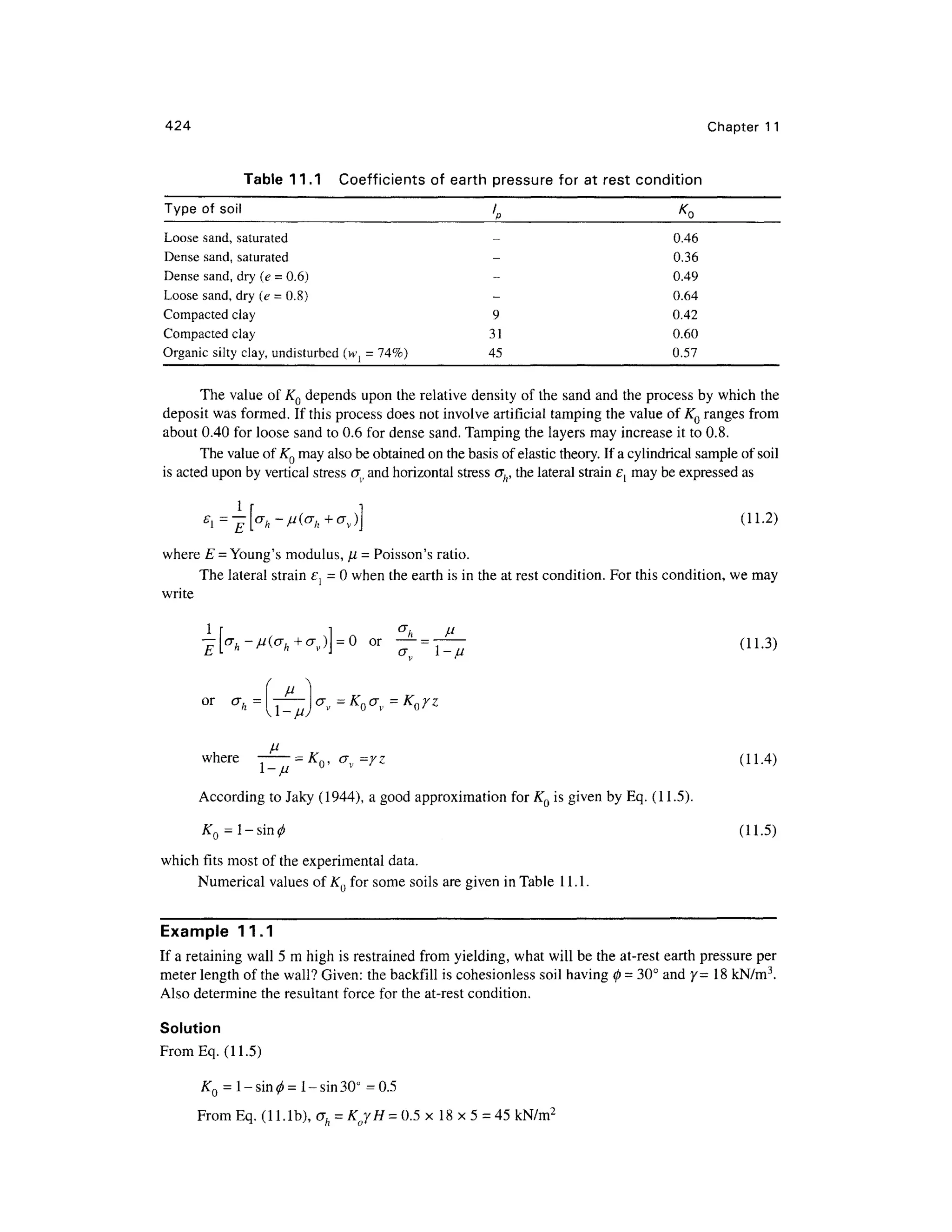
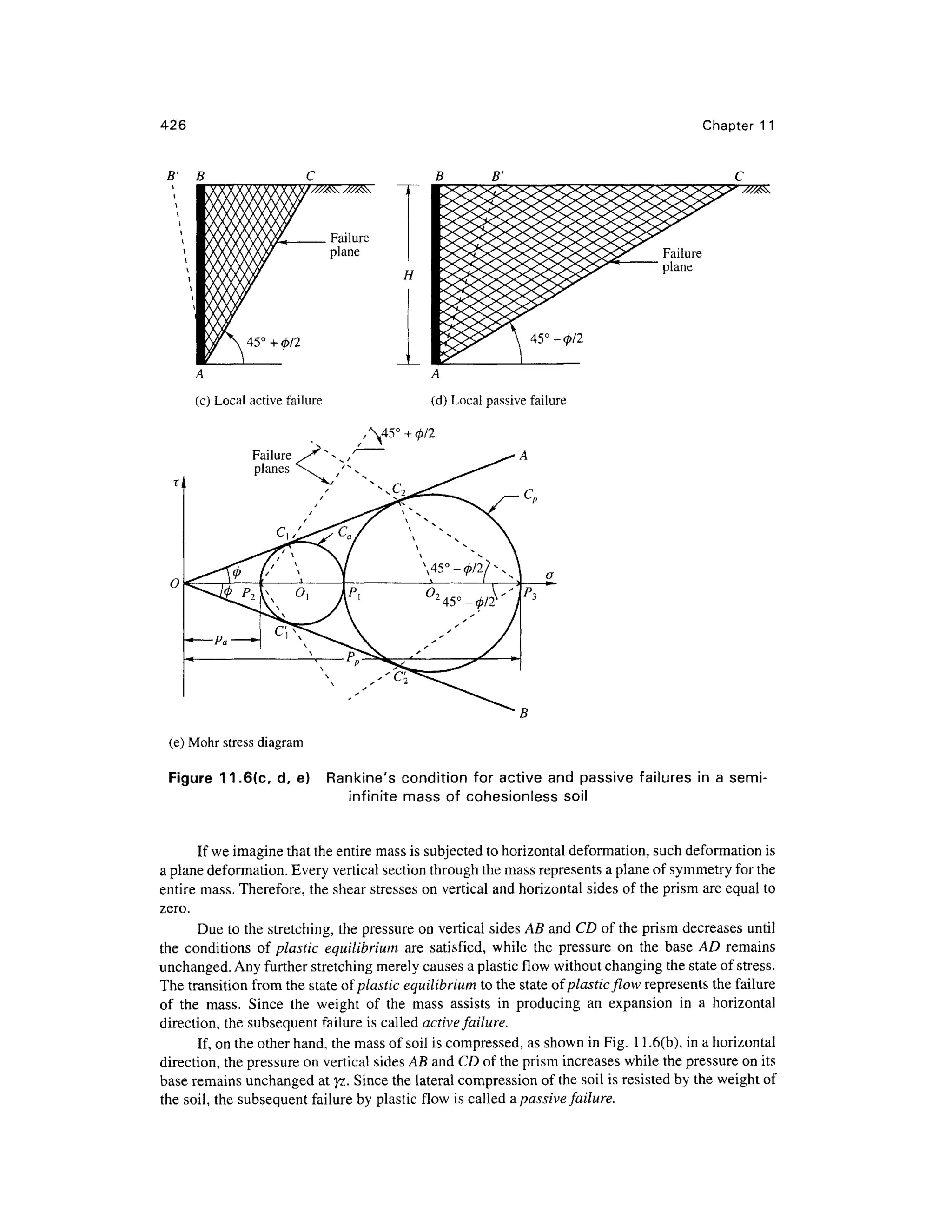
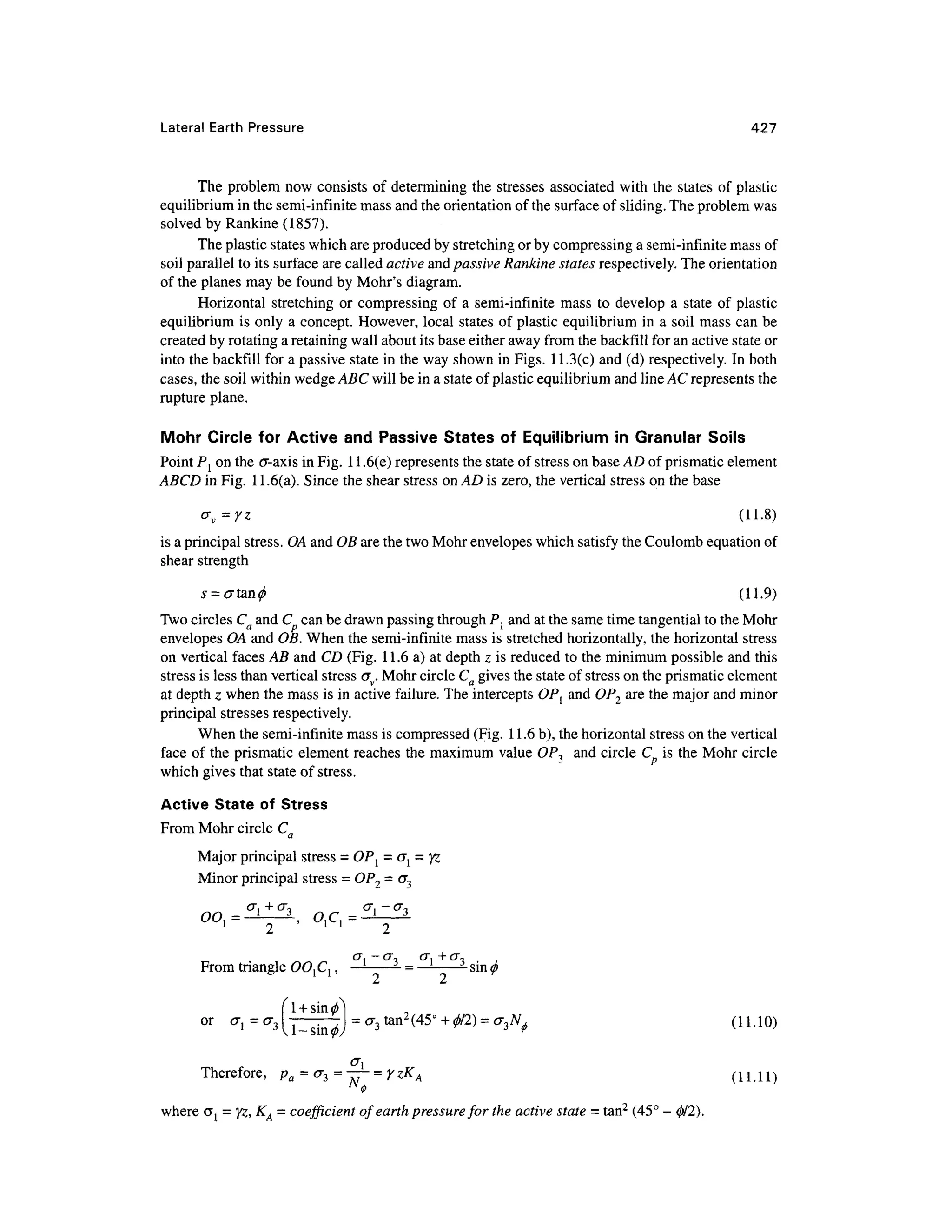
447. 428 Chapter 1 1
From point Pr draw a line parallel to the base AD on which (7 { acts . Since this line coincide s
with the cr-axis, point P9 is the origin of planes. Lines P2C{ an d P^C giye tne
orientations of the
failure planes. They make an angle of 45° + 0/2 with the cr-axis. The lines drawn parallel to the lines
P2Cj and P2C'{ i n Fig. 11.6(a ) give the shear lines along which the soil slips in the plastic state. The
angle between a pair of conjugate shear lines is (90° - 0).
Passive Stat e o f Stress
C i s the Mohr circle in Fig. (11.6e) for the passive state and P3 is the origin of planes.
Major principal stress = (j } = p= OP^
Minor principal stress = (73 = OPl = yz.
From triangle OO^C2, o{ = yzN^
Since <J l - p an d<J 3 = yz, we have
n -yzN:-r7K (] ] ]?}
i n * Q) i f t L L * . £ j
where K = coefficient o f earth pressure for th e passive state = tan2
(45° + 0/2).
The shea r failur e line s are P3C2 an d P3C^ an d they make a n angle o f 45° - 0/ 2 with the
horizontal. The shea r failure line s are drawn parallel to P3C2 an d P3C'2 i n Fig. 11.6(b) . The angle
between any pair of conjugate shear lines is (90° + 0).
11.5 RANKINE' S EARTH PRESSUR E AGAINST SMOOTH
VERTICAL WALL WITH COHESIONLES S BACKFIL L
Backfill Horizontal-Activ e Eart h Pressur e
Section AB i n Fig. 11.6(a ) in a semi-infinite mass is replaced by a smooth wall AB in Fig. 11.7(a) .
The latera l pressure actin g against smooth wal l AB i s due t o the mass o f soi l ABC abov e
failure lin e A C whic h make s a n angl e o f 45 ° + 0/ 2 wit h th e horizontal . Th e latera l pressur e
distribution o n wal l AB o f heigh t H increase s i n simpl e proportio n t o depth . The pressur e act s
normal to the wall AB [Fig . 11.7(b)] .
The lateral active pressure at A is
(11.13)
B' B
W
45° +
(a) (b )
Figure 11. 7 Rankine' s activ e eart h pressur e i n cohesionless soi l

448. Lateral Earth Pressur e 429
The total pressure o n AB is therefore
HH
z d Z = K
(11.14)
o o
where, K A = tan2
(45° -
1 +sin^ V i
Pa acts at a height H/3 above the base of the wall.
Backfill Horizontal-Passiv e Eart h Pressur e
If wall AB is pushed into the mass to such an extent as to impart uniform compression throughout
the mass, soil wedge ABC in Fig. 11.8(a ) will be in Rankine's passive state of plastic equilibrium.
The inner rupture plane AC makes an angle 45° + 0/2 with the vertical AB. The pressure distribution
on wall AB is linear as shown in Fig. 11.8(b) .
The passive pressure p a t A is
PP=YHKp
the total pressure against the wall is
P
P= (11.15)
where, K p = tan2
(45° +
1 +sin ^
1 -sin 6
Relationship between Kp and KA
The ratio of Kp an d KA may be written as
Kp tan 2
(45c
KA tan 2
(45c (11.16)
B B'
Inner rupture plane
' W
(a) (b)
Figure 11.8 Rankine' s passive earth pressure in cohesionless soil

449. 430 Chapter 1 1
H
P + P
1
a Tr
w
45° + 0/2
(a) Retaining wall
'-*
H- v bnKA
(b) Pressure distribution
H
Figure 1 1.
9 Rankine' s active pressure under submerged conditio n in cohesionless
soil
For example, if 0 = 30°, we have,
K
P
-7T1
= tan4
600
= 9 , o r K p= 9KA
KA
This simple demonstration indicates that the value of Kp i s quite large compared t o K A.
Active Eart h Pressure-Backfill Soi l Submerged with the Surfac e Horizontal
When the backfill is fully submerged , two types of pressures act on wall AB. (Fig . 1 1.9) They are
1. Th e active earth pressure due to the submerged weight of soil
2. Th e lateral pressure due to water
At any depth z the total unit pressure on the wall is
At depth z = H, we have
~p~ = y,HK. + y H
r a ID A ' w
where y b i s the submerge d uni t weight of soil and y w th e unit weight of water. The tota l pressur e
acting on the wall at a height H/3 above the base is
(11.17)
Active Eart h Pressure-Backfill Partly Submerged with a Uniform Surcharg e Load
The groun d water table is at a depth of Hl belo w th e surface and the soil abov e thi s level has an
effective moist unit weight of y. The soil below the water table is submerged with a submerged unit
weight yb. In this case, the total unit pressure may be expressed a s given below.
At depth Hl a t the level of the water table

450. Lateral Earth Pressur e 431
At depth H we have
or (11.18)
The pressure distribution is given in Fig. 1 1.10(b). It is assumed that the value of 0 remains
the same throughout the depth H.
From Fig. 1 1.10(b), we may say that the total pressure P a actin g per unit length of the wall
may be written as equal to
(11.19)
The point of application of P a abov e the base of the wall can be found by taking moments of
all the forces acting on the wall about A.
Sloping Surface-Activ e Eart h Pressur e
Figure 1 1.1 1(a) shows a smooth vertical wall with a sloping backfill of cohesionless soil . As in the
case of a horizontal backfill, the active state of plastic equilibrium can be developed i n the backfill
by rotating the wall about A away from the backfill. Let AC be the rupture line and the soil within
the wedge ABC be in an active state of plastic equilibrium.
Consider a rhombic element E within the plastic zone ABC which is shown to a larger scal e
outside. The base of the element is parallel to the backfill surface which is inclined at an angle /3 to
the horizontal. The horizontal width of the element is taken as unity.
Leto~ v = the vertical stress acting on an elemental length ab =
(7l = the lateral pressure acting on vertical surface be of the element
The vertical stresso~ v can be resolved into components<3 n the normal stress and t the shear
stress on surface ab of element E. We may now write
H
g/unit area
I I I 1 I I
I
Pa (total) =
(a) Retaining wall (b) Pressure distribution
Figure 11.10 Rankine' s active pressure in cohesionless backfill unde r partl y
submerged conditio n with surcharge load

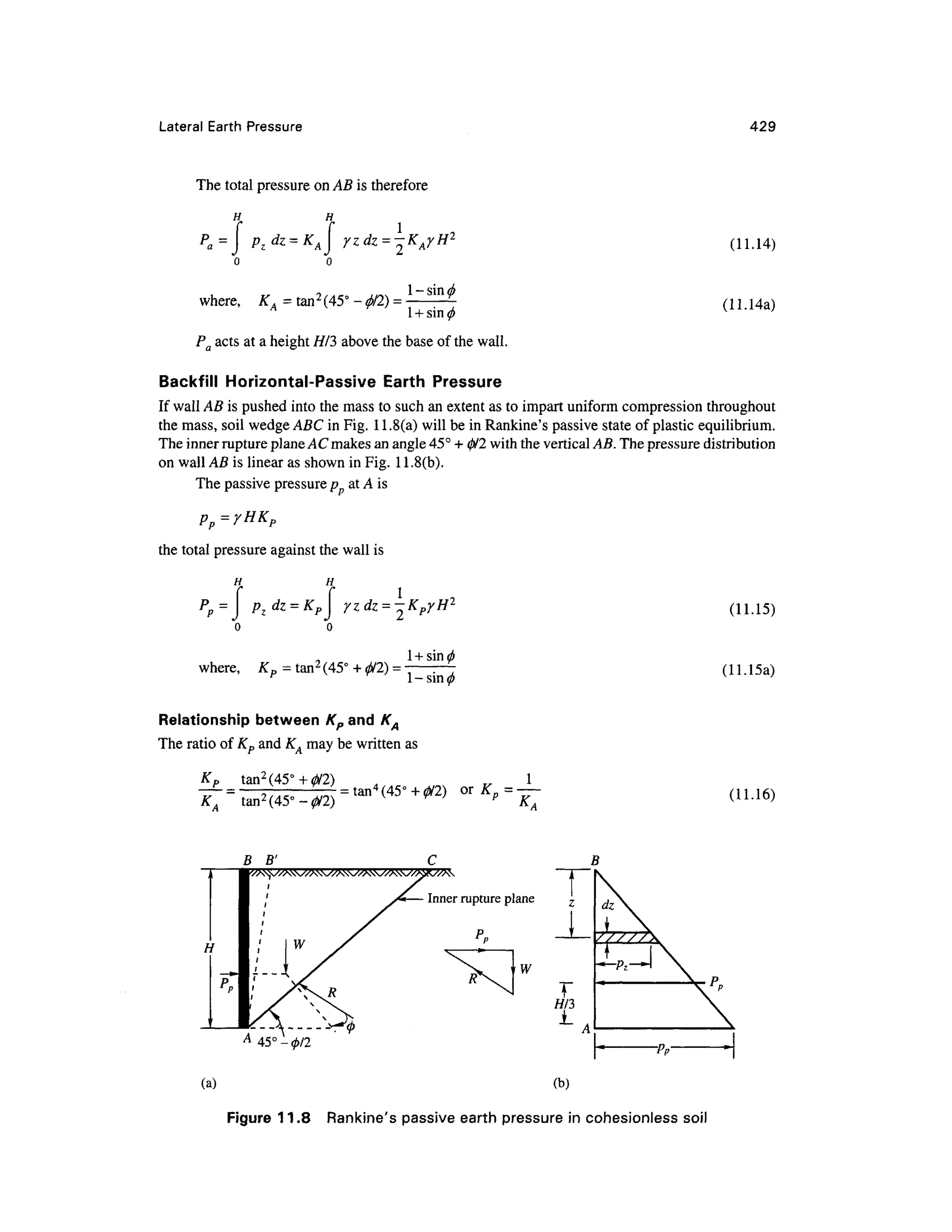
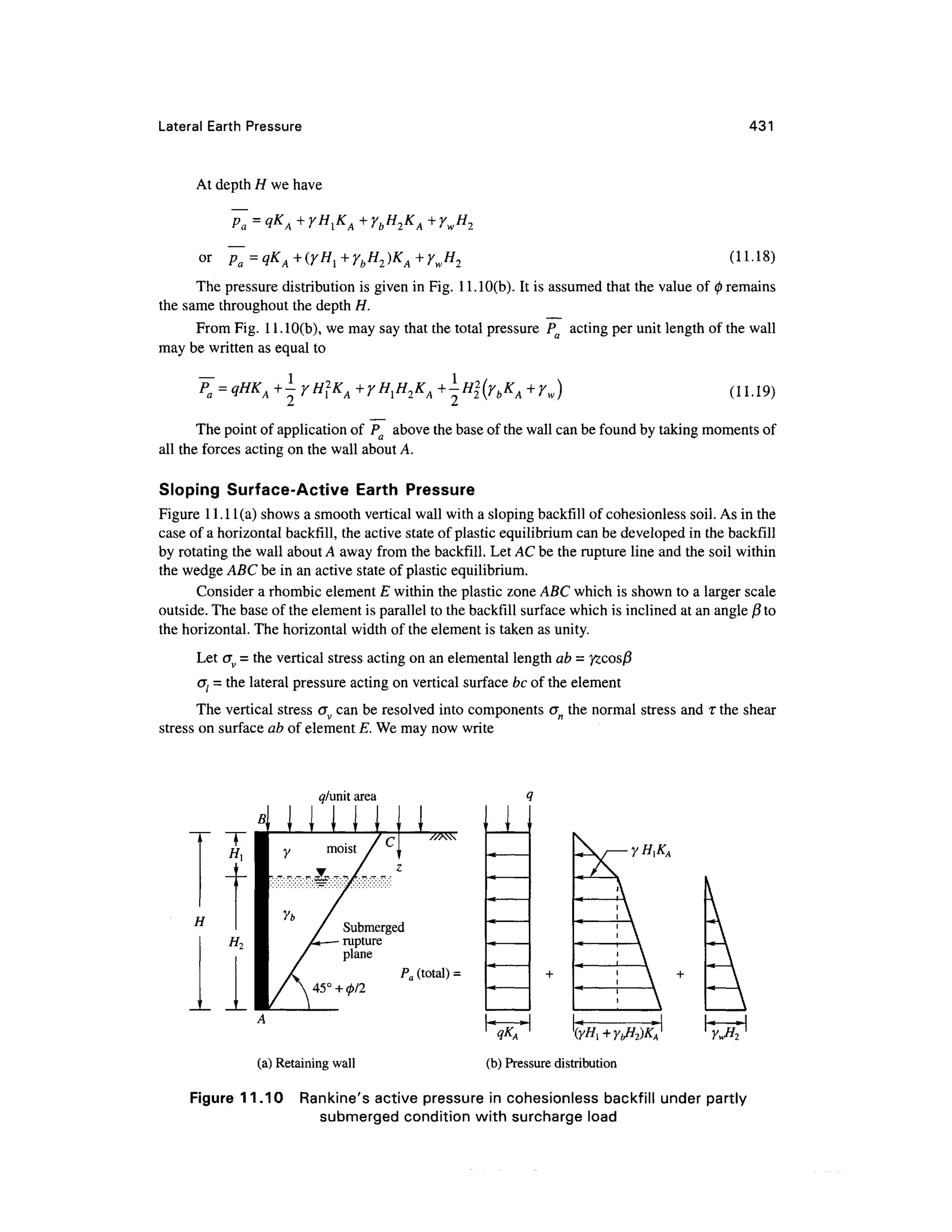
451. 432 Chapter 1 1
H
(a) Retaining wall (b) Pressure distribution
O CT 3 0 , O n O]
(c) Mohr diagram
Figure 11.1 1 Rankine' s active pressur e for a sloping cohesionles s backfil l
n - <J v cos fi = yz cos /?cos fl= y z cos 2
j3
T = a sin/ ? =
(11.20)
(11.21)
A Mohr diagram can be drawn as shown in Fig. 11. 1 l(c). Here , length OA = yzcos/3 make s
an angle (3 with the (T-axis. OD = on - yzcos 2
/3 and AD = T=yzcosf} sin/3 . OM is the Mohr envelope
making an angle 0 with the <7-axis. Now Mohr circle C} can be drawn passing through point A and
at the same time tangential to envelope OM. This circle cuts line OA at point B and the CT-axi
s a
t E
andF.
Now OB = the lateral pressure ol =pa in the active state.
The principal stresses are
OF = CTj and O E = a3
The following relationships can be expressed wit h reference to the Mohr diagram.
BC = CA =
— -
l -sm2
j3

452. Lateral Earth Pressure 433
= OC-BC =
2
cr, +CT , cr, + cr,
i
2 2
Now we have (after simplification)
cos 0 -
T] cos2
ft -cos
crv yzcosfi cos 0+J cos2
fi -cos2
0
or
cos B- A/cos2
/?- cos2
(b
- v
cos/?+cos2
/?-cos
where, K. = cos fi x
(11.22)
(11.23)
(11.24)
is calle d a s th e coefficient o f earth pressure fo r th e activ e stat e o r th e activ e eart h pressur e
coefficient.
The pressure distribution on the wall is shown in Fig. 1 1 . 1l(b). The active pressure at depth H
is
which acts parallel to the surface. The total pressure PQ per unit length of the wall is
(11.25)
which act s a t a height H/3 fro m th e bas e o f the wal l and paralle l t o th e slopin g surfac e o f th e
backfill.
(a) Retaining wall (b ) Pressure distribution
Figure 11.1 2 Rankine' s passive pressure in sloping cohesionless backfil l

453. 434 Chapter 1 1
Sloping Surface-Passiv e Eart h Pressur e (Fig . 11.12 )
An equation for P fo r a sloping backfill surface can be developed i n the same way as for an active
case. The equation for P ma y be expressed as
(11.26)
n cos fi +Jcos2
fl- cos 2
0
where, K p
= cos]3x/
cos /3 - ^cos2
j3- cos2
0
P act s at a height H/3 abov e point A and parallel to the sloping surface.
(11.27)
Example 11. 2
A cantilever retaining wall of 7 meter height (Fig. Ex. 11.2) retains sand. The properties o f the sand
are: e - 0.5 , 0 =30° and G^ = 2.7. Using Rankine's theory determine the active earth pressure at the
base when the backfill is (i) dry, (ii) saturated and (iii) submerged, and also the resultant active force
in each case . In addition determine the total water pressure under the submerged condition.
Solution
e = 0.
5 an
d G= 2.7, y, = -^= —— x 9.81 =17.66 kN/m3
d
l + e1 + 0.5
Saturated unit weight
Backfill submerge d
Backfill saturate d
Water pressur e
pa = 48.81 kN/m"
= 68.67 kN/m2
= Pw
Figure Ex. 11.2

454. Lateral Earth Pressur e 43 5
=
sat
l + e1 + 0.5
Submerged unit weight
rb = rsal -rw= 20.92-9.81 =11.1 kN/m3
l-sin^ 1 - sin 30° 1
For* =30, * A
Active earth pressure at the base is
(i) fo r dry backfill
Pa =
P = -K
A r,H 2
= -
x 41.2x7 =144.2 kN/mofwall
a r A ' a rj
(ii) fo r saturated backfil l
Pa = K
A Ysat H = -x20.92 x 7 = 48.8 1kN/m2
p = -x 48.8 1x7 = 170.85 kN/ m of wall
a
2
(in) fo r submerged backfill
Submerged soi l pressure
Pa
= K
/JbH
= -x 11.1 x7=25.9 kN/m2
P = - x 25.9 x 7 =90.65 kN/ m of wall
a
2
Water pressure
pw = ywH = 9.8 1x 7=68.67 kN/m 2
Pw=-YwH2
= -x 9.81 x72
=240.35 kN/mofwal l
Example 11. 3
For the earth retaining structure shown in Fig. Ex. 11.3, construct the earth pressure diagram for the
active state and determine the total thrust per unit length of the wall.
Solution
1-sin 30° 1
For<z)=30°, K A : - = -
G Y 265 i
Dry unit weight YH = —^
^ = —: x
62.4 =100.22 lb/ fr
y d
l + e1 + 0.6
5

455. 436 Chapter 1 1
q = 292 lb/ft 2
J I U J J H J
E--
//A
|
=i
32.8ft> >
1
1
J
1
9.8ft
Sand G s =2.65
e = 0.65
0 = 30°
(a) Given syste m
Pl Pi P3
(b) Pressure diagram
Figure Ex . 11.3
(Gs-l)yw 2.65- 1
7b =-^—- =T
-^X 62.4 =62.4 ,b/f,3
Assuming the soil above the water table is dry, [Refer to Fig. Ex. 11.3(b)] .
P! = KAydHl = - x 100.22x9.8 = 327.39 lb/ft 2
p2 = KAybH2 = -x 62.4 x 23 =478.4 lb/ft 2
p3 = KAxq = -x292= 97.33 lb/ft 2
P4 = (K
A^wrw
H
2 = 1x62.4x23 =1435.2 lb/ft 2
Total thrust = summation of the areas of the different part s of the pressure diagra m
1 1 1
= ^PiHl+plH2+-p2H2+p3(Hl+H2) + -p4H2
= -x 327.39 x9.8 + 327.39 x 23 + -
x 478.4 x 23 + 97.33(32.8) + -
x 1435.2x23
2 2 2
= 34,333 lb/f t = 34.3 kips/ft o f wall
Example 11. 4
A retaining wall with a vertical back of height 7.32 msupports a cohesionless soil of unit weight
17.3 kN/m 3
an d a n angle o f shearing resistance 0 = 30°. The surfac e o f th e soi l i s horizontal .
Determine th e magnitud e an d directio n o f th e activ e thrus t pe r mete r o f wal l usin g Rankin e
theory.

456. Lateral Earth Pressure 437
Solution
For the condition given here, Rankine's theory disregards the friction between the soil and the back
of the wall.
The coefficient of active earth pressure KA i s
1-sind l-sin30 ° 1
Tf T_
A
1 + sin^ 1 +sin 30° 3
The lateral active thrust Pa is
Pa = -K
AyH2
= -x-
x 17.3(7.32)2
= 154.5 kN/m
Example 11. 5
A rigid retaining wall 5 m high supports a backfill of cohesionless soi l with 0= 30°. The water table
is below th e base o f the wall. The backfill is dry and has a unit weight of 1 8 kN/m3
. Determine
Rankine's passive earth pressure per meter length of the wall (Fig. Ex. 11.5).
Solution
FromEq. (11.15a)
Kp =
1 + sin^ 1 + sin 30° 1 + 0.5
in^ l-sin30 ° 1-0. 5
At the base level, the passive earth pressure is
pp = K pyH = 3x18x5 = 270 kN/m2
FromEq. (11.15 )
Pp=- KPy H = -x 3 x1 8 x5 = 675 kN/m length of wall
The pressure distributio n is given in Fig. Ex. 1 1.5.
Pressure distributio n
Figure Ex. 11.5

457. 438 Chapte r 1 1
Example 11. 6
A counterfor t wall o f 1 0 m heigh t retains a non-cohesive backfill . The voi d rati o an d angl e o f
internal friction of the backfill respectively are 0.70 and 30° in the loose state and they are 0.40 and
40° in the dense state. Calculate and compare active and passive earth pressures fo r both the cases.
Take the specific gravity of solids as 2.7.
Solution
(i) In the loose state, e - 0.7 0 which gives
/""* - .
r i—j
= _I^L = _ _ x 9 gj =15 6 kN/m3
d
l + e1 + 0.7
c j. ™ ° v l-sin 0 1-si n 30° 1 1
For 0 =3 0, K , - =
= — ,and^ 0 =
= 3
' A - i * ' 1 * O /" o O i TS
1 +sin 30 3 K,
Max. pa = KAydH = - x 15.6 x 10 =52 kN/m2
Max. p = KpydH = 3 x 15.6 x 10 =468 kN/m2
(ii) In the dense state, e = 0.40, which gives,
Y = -22—x9.81 =18.92 kN/m3
d
1 + 0.4
1-sin 40° 1
For 0 = 40°, K= - — — = 0.217, K p = - — = 4.6
y A
1 +sin 40° p
K. f
Max.pfl = K AydH = 0.217x18.92x10 = 41.1 kN/m2
and Max. p= 4.6 x 18.92 x 10 =870.3 kN/m2
Comment: Th e compariso n o f the results indicate s tha t densification of soi l decrease s th e
active earth pressure and increases the passive earth pressure. This is advantageous in the sense that
active earth pressure is a disturbing force and passive earth pressure is a resisting force.
Example 11. 7
A wall of 8 m height retains san d having a density of 1.936 Mg/m3
and an angle of internal frictio n
of 34°. If the surface of the backfill slopes upwards at 15° to the horizontal, fin d the active thrust per
unit length of the wall. Use Rankine's conditions.
Solution
There can be two solutions: analytical and graphical. The analytical solution can be obtained fro m
Eqs. (11.25 ) and (11.24) viz.,

458. Lateral Earth Pressure 439
Figure Ex. 11.7 a
where K. = cos ft x
cos/?- ycos2
ft - cos 2
COS/?+ yCOS2
ft - COS 2
(f)
where ft = 15°, cos/? = 0.9659 an d cos 2
ft = 0.933
and ^ = 34° give s cos 2
(/) = 0.688
0.966 -VO.933- 0.688
= 0.3 11
Hence K A = 0.966 x .
A
0.96 6 + VO.933 -0.688
y = 1.936x9.81 =19.0 kN/m3
Hence P a = -x0.311x!9(8)2
= 189 kN/ m wall
Graphical Solutio n
Vertical stress at a depth z = 8 m is
7/fcos/?=19x8xcosl5° = 147 kN/m2
Now draw the Mohr envelope at an angle of 34° and the ground line at an angle of 15 ° with
the horizontal axis as shown in Fig. Ex. 1 1.7b.
Using a suitable scale plot OPl = 147 kN/m2
.
(i) th e center of circle C lies on the horizontal axis,
(ii) th e circle passes through point Pr and
(iii) th e circle is tangent to the Mohr envelope

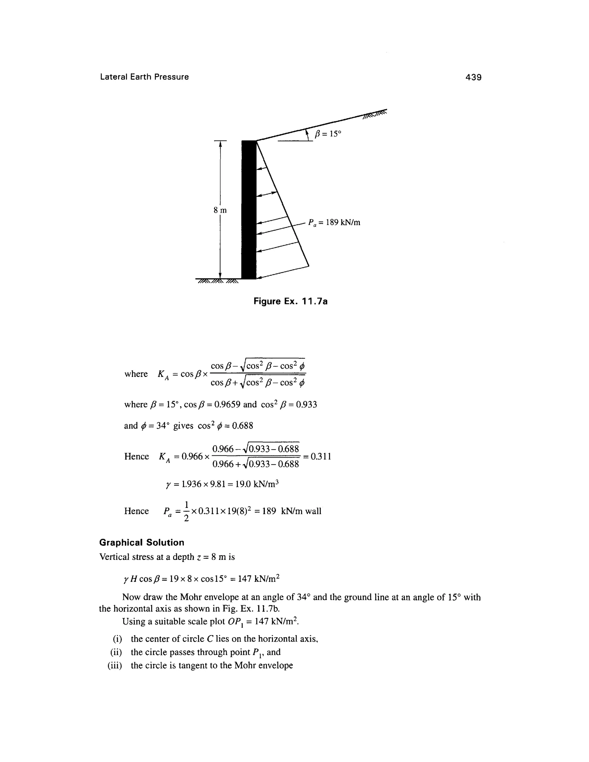
459. 440 Chapter 1 1
Ground line
16 18 x 1 0
Pressure kN/m
Figure Ex. 11.7 b
The point P2 at which the circle cuts the ground line represents the lateral earth pressure. The length
OP2 measures 47.5 kN/m 2
.
Hence the active thrust per unit length, P a = -x 47.5 x 8 =190 kN/m
1 1 .
6 RANKINE' S ACTIVE EARTH PRESSURE WIT H COHESIVE
BACKFILL
In Fig. 1 1.1 3(a
) is shown a prismatic element in a semi-infinite mass with a horizontal surface. The
vertical pressure on the base AD of the element at depth z is
The horizontal pressure on the element when the mass is in a state of plastic equilibrium may
be determined b y making use of Mohr's stres s diagram [Fig. 1 1.13(b)]
.
Mohr envelopes O'A and O'E for cohesive soils are expressed by Coulomb's equation
s - c +tan 0 (11.28)
Point P j o n the cr-axi s represents th e stat e of stres s o n the base of the prismati c element .
When the mass is in the active state cr, is the major principal stress Cfj . The horizontal stress oh is the
minor principal stres s <7 3. The Moh r circle of stress C a passing throug h P{ an d tangentia l to th e
Mohr envelope s O'A an d O'B represent s th e stres s condition s i n th e activ e state . Th e relatio n
between the two principal stresses may be expressed by the expression
(11.29)
(11.30)
<7, = <7, A
1 J V v y
SubstitutingO" , = 72,<7 3 =pa and transposin g we have
rz 2 c

460. Lateral Eart h Pressur e 441
45° + 0/2
Stretching
45° + 0/2
D B
C A
'" ,-; ,-" ,-",-• ; t -
^A'-^ i" j Z:J A'
Tensile
zone
Failure shear lines
(a) Semi-infinite mass
Shear lines
(b) Mohr diagram
Figure 11.1 3 Activ e eart h pressure of cohesive soil with horizontal backfil l o n a
vertical wal l
The active pressure pa = 0 when
yz 2c rt
(11.31)
that is, pa i s zero at depth z, such that
At depth z = 0, the pressure pa i s
2c
Pa - JTf ^
(11.32)
(11.33)

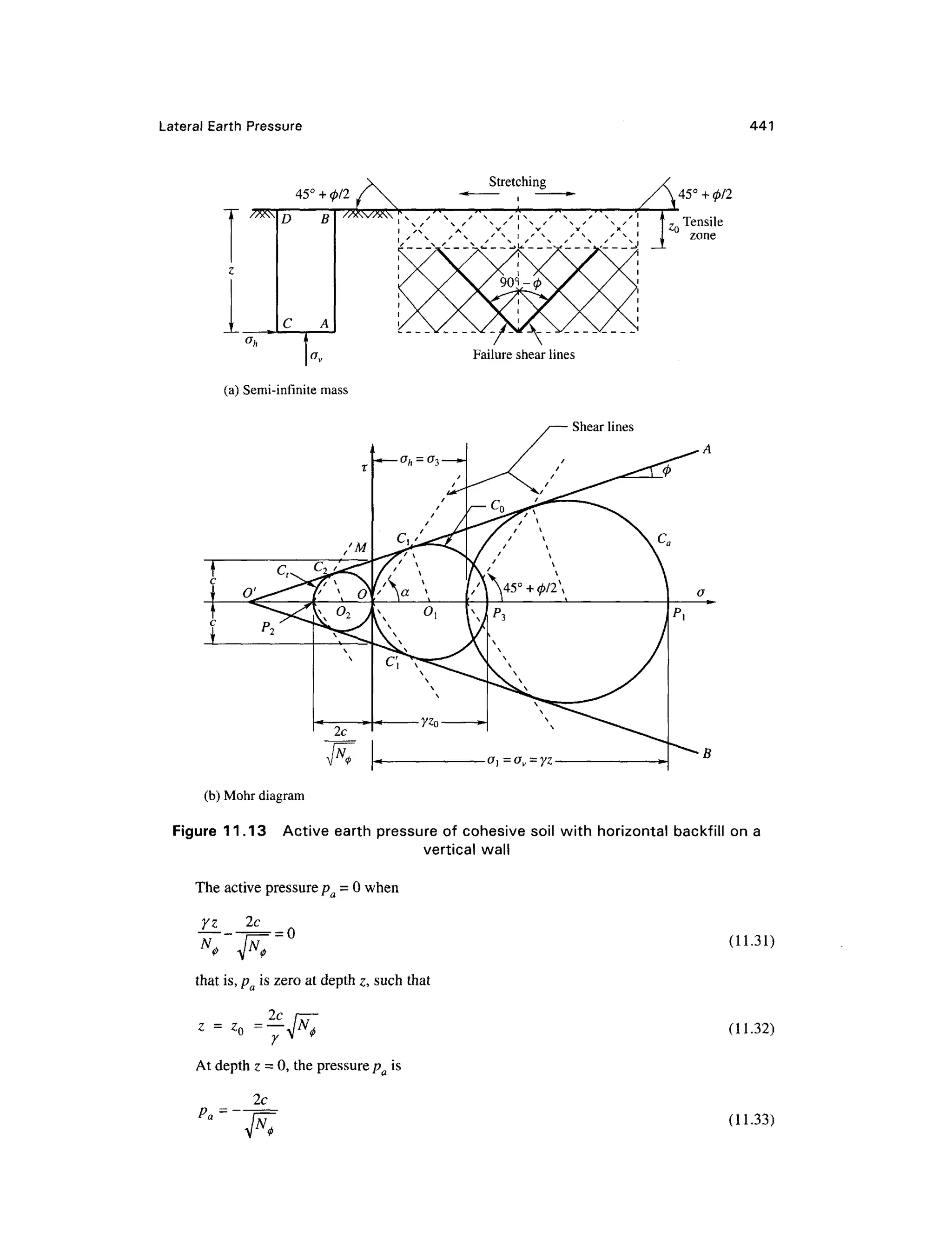
461. 442 Chapte r 1 1
Equations (1 1 .32) and (1 1.33) indicate that the active pressure pa i s tensile between dept h 0
and ZQ. The Eqs. ( 1 1.32) and (1 1.33) can also be obtained fro m Mohr circles CQ and Ct respectively .
Shear Line s Patter n
The shear lines are shown in Fig. 1 1 . 13(a). Up to depth ZQ they are shown dotted to indicate that this
zone is in tension.
Total Active Eart h Pressur e o n a Vertical Sectio n
If AB is the vertical section [1 1.14(a)], the active pressure distribution against this section of height
H is shown in Fig. 11.1 4(b) as per Eq. (1 1.30). The total pressure against the section i s
H H H
yz 2c
Pa = PZdz
= ~dz- -r
= = dz
o 0 ' 0 V A
0
H
The shaded are a in Fig. 1 1.14(b) gives the total pressure Pa. If the wall has a height
the total earth pressure is equal to zero. This indicates that a vertical bank of height smaller than H
can stand without lateral support. //, is called the critical depth. However , the pressure agains t the
wall increases fro m - 2c/JN^ a t the top to + 2c/jN^ a t depth //,, whereas on the vertical face of
an unsupported bank the normal stress is zero at every point. Because of this difference, the greatest
depth of which a cut can be excavated without lateral support for its vertical sides is slightly smaller
than H c.
For soft clay, 0 =0, and N^= 1
therefore, P a
= ±yH2
-2cH (11.36 )
4c
and HC
=
~^ (1L37 )
Soil does not resist any tension and as such it is quite unlikely that the soil would adhere to the
wall within the tension zone of depth z0 producing cracks i n the soil. It is commonl y assume d that
the active eart h pressure is represented b y the shaded are a in Fig. 1 1.14(c).
The tota l pressure o n wal l AB i s equal to the are a o f the triangle in Fig. 11.14(c) whic h is
equal to
1 yH 2c
D 1 yH 2c „ 2c
or F =
" H
"

462. Lateral Eart h Pressure 443
Surcharge load q/unit area
B l l C
2c
8
jH 2c
q
q
%v %N
*
(a) (b ) (c ) (d )
Figure 11.1 4 Activ e eart h pressur e on vertical sections in cohesive soil s
Simplifying, w e have
1 2c 2
2 N
*
For soft clay, 0 = 0
Pa = -yHl
It may be noted that KA = IN^
(11.38c)
(11.39)
Effect o f Surcharg e an d Water Tabl e
Effect o f Surcharge
When a surcharge load q per unit area acts on the surface, the lateral pressur e o n the wall due to
surcharge remain s constan t wit h dept h a s show n i n Fig. 11.14(d ) fo r th e activ e condition . Th e
lateral pressure due to a surcharge under the active state may be written as
The total active pressure due to a surcharge load is,
n _&
(11.40)
Effect o f Wate r Tabl e
If the soil is partly submerged, the submerged uni t weight below the water table will have to be
taken into account in both the active and passive states .

463. 444 Chapter 1 1
Figure 11.15(a) shows the case of a wall in the active state with cohesive material as backfill.
The water table is at a depth of Hl belo w the top of the wall. The depth of water is //2.
The lateral pressure on the wall due to partial submergence is due to soil and water as shown
in Fig. 11.15(b) . The pressure due to soil = area of the figure ocebo.
The total pressure due to soil
Pa = oab + acdb+ bde
1 2c
NA JN.
2c
N (11.41)
2C r—
After substituting for zn = — N
and simplifying we have
1
p ( v jr2 , ,
A — » • » , / - - * - * 1 l t
2c
The total pressure on the wall due to water is
p v JJ2
~ n
2c2
(11.42)
(11.43)
The poin t o f applicatio n o f P a ca n b e determine d withou t an y difficulty . Th e poin t o f
application P W i s at a height of H2/3 fro m the base of the wall.
Cohesive soil
7b
T
H2/3
_L
Pressure due
to water
(a) Retaining wall (b) Pressure distribution
Figure 11.1 5 Effec t o f wate r table o n lateral earth pressur e

464. Lateral Earth Pressur e 44 5
If the backfill material is cohesionless, th e terms containing cohesion c in Eq. (11.42) reduce
to zero.
Example 11. 8
A retaining wall has a vertical back and is 7.32 m high. The soil is sandy loam of unit weight 17.
3
kN/m3
. It has a cohesion o f 1 2 kN/m2
and 0 = 20°. Neglecting wall friction, determine the active
thrust on the wall. The upper surface of the fill is horizontal.
Solution
(Refer to Fig. 11.14 )
When th e materia l exhibit s cohesion , th e pressur e o n th e wal l a t a dept h z i s give n b y
(Eq. 11.30 )
where K J_^iT = — = 0.49, I K 0 .7
v A
1-sin 20°
1 +sin 20°
When the depth is small the expression fo r z is negative because of the effect o f cohesion u p to a
theoretical dept h z0. The soil is in tension and the soil draws away from the wall.
-— I —-—I
y v Y
1 + sin(f) i
where K p = 7- 7 =2.04, an d JK P = 1.43
p
- * p
2x12
Therefore Z Q = "TTT" x
1-43 =1-98 m
The lateral pressure at the surface (z = 0) is
D = -2cJxT = -2 x 12 x0.7 =-16.8 kN/m2
* u V •* »
The negative sign indicates tension .
The lateral pressure at the base of the wall (z = 7.32 m) is
pa = 17.3 x7.32 x 0.49 -16.8 =45.25 kN/m2
Theoretically th e area of the upper triangle i n Fig. 11.14(b ) to the left o f the pressure axis
represents a tensile force which should be subtracted from the compressive forc e on the lower part
of the wall below the depth ZQ. Since tension cannot be applied physically between the soil and the
wall, this tensile force is neglected. It is therefore commonly assumed that the active earth pressure
is represented b y the shaded area in Fig. 1 1 . 14(c). The total pressure on the wall is equal to the area
of the triangle in Fig. 1 1.14(c).
= -(17.3 x7.32 x 0.49 - 2 x12 x0.7) (7.32- 1.98) = 120.8 kN/m

465. 446 Chapter 1 1
Example 11. 9
Find the resultant thrust on the wall in Ex. 11.8 if the drains are blocked and water builds up behind
the wall until the water table reaches a height of 2.75 m above the bottom of the wall.
Solution
For details refer to Fig. 11.15 .
Per this figure,
Hl = 7.32 - 2.75 = 4.57 m, H2 = 2.75 m, H, - Z 0 = 4.57 -1.98 = 2.59 m
The base pressure is detailed in Fig. 11.15(b )
(1) Y SatH
K
A - 2c
JK~A = !7.3x4.57x0.49-2x12x0.7 = 21.94 kN/m2
(2) 7 bH2KA - (17.3 -9.8l)x 2.75x0.49 =10.1 kN/m2
(3) y w H2 = 9.81 x2.75 = 27 kN/m2
The total pressure = Pa = pressure due to soil + water
From Eqs. (11.41), (11.43), and Fig. 11.15(b )
Pa = oab + acdb+ bde+ bef
1 1 1
= - x 2.59 x 21.94 + 2.75 x21.94 + -x 2.75 x10.1 + - x 2.75 x 27
= 28.41 + 60.34 + 13.89 +37.13 = 139.7 kN/m or say 14 0 kN/m
The point of application of Pa may be found by taking moments of each area and Pa about the
base. Let h be the height of Pa above the base. Now
1 97 5 97 5 3713x97 5
140x^ = 28.41 -X2.5 9 +2.75 + 60.34 x —
+ 13.89 x —
+
3 2 3 3
16.8 kN/m2
ysat= 17.3 kN/m
0 = 20
°
c= 1 2 kN/m2
P,, =14 0 kN/m
Figure Ex. 11.9

466. Lateral Earth Pressure 447
or
= 102.65 +83.0 +12.7 +34.0 = 232.4
232.4
140
= 1.66m
Example 11.1 0
A rigid retaining wall 19.69 ft high has a saturated backfill of soft cla y soil. The properties of the
clay soil are ysat = 111.76 lb/ft3
, and unit cohesion cu = 376 lb/ft2
. Determine (a) the expected depth
of the tensile crack in the soil (b) the active earth pressure before the occurrence of the tensile crack,
and (c) the active pressure after the occurrence of the tensile crack. Neglect the effect o f water that
may collect in the crack.
Solution
At z = 0, p a = -2c = -2 x 376 = -752 lb/ft 2
sinc e 0 =0
Atz = H,p a = yH-2c=l.16x19.6 9 - 2 x 376 =1449 lb/ft2
(a) From Eq. (11.32), the depth of the tensile crack z0 is (for 0=0)
_2c _ 2x376
Z
° ~ y~ 111.7 6
= 6.73 ft
(b) The active earth pressure before the crack occurs.
Use Eq. (11.36) for computing Pa
1
19.69 f t
y=111.76 lb/ft3
cu = 376 lb/ft2
752 lb/ft 2
6.73 f t
1449 lb/ft 2
(a) (b)
Figure Ex. 11.10

467. 448 Chapte r 1 1
since KA = 1 for 0 = 0. Substituting, we have
Pa = -
x 1 1 1.76x(19.69)
2
-2 x 376x19.69 = 21,664 -14,807 = 6857 lb/ ft
(c) Pa after the occurrence o f a tensile crack.
UseEq. (11.38a),
Substituting
pa = 1(
1 11.76 x 19.69- 2 x 376) (19.69- 6.73) = 9387 Ib/f t
Example 11.1 1
A rigid retaining wall of 6 m height (Fig. Ex. 11.11 ) has two layers of backfill. The top layer to a
depth of 1.5 m is sandy clay having 0=20°, c= 12.15 kN/m
2
and y-16.4 kN/m3
. The bottom layer
is sand having 0 = 30°, c= 0, and y- 17.25 kN/m3
.
Determine the total active earth pressure acting on the wall and draw the pressure distribution
diagram.
Solution
For the top layer,
70 1
KA = tan2
45 ° - — = 0.49, K p = —5— = 2.0
4
A
2 p
0.4 9
The dept h of the tensile zone, Z Q is
2c r— 2X12.15VI0 4
16.4
=112m
Since th e dept h o f th e sand y cla y laye r i s 1. 5 m, whic h i s les s tha n Z Q, th e tensil e crac k
develops onl y to a depth of 1. 5 m.
KA fo r the sandy layer is
At a depth z= 1.5, the vertical pressure G V is
crv = yz= 16.4 x 1.5 = 24.6 kN/m2
The active pressure is
p = KAvz = -x24.6 =8.2 kN/m2
a A
3
At a depth of 6 m, the effective vertical pressure is

468. Lateral Earth Pressure 449
GL
V/V/AV/V/
1.5m
4.5m
Figure Ex . 11.11
<jv = 1.5 x 16.4 + 4.5 x17.25 = 24.6 + 77.63 = 102.23 kN/m2
The active pressure pa i s
pa = KA av = -x 102.23 = 34.1 kN/m2
The pressure distribution diagram is given in Fig. Ex. 11.11 .
8.2 kN/m2
•34.1 kN/m2
1 1 .
7 RANKINE' S PASSIV E EART H PRESSUR E WITH COHESIV E
BACKFILL
If the wall AB in Fig. 1 1 . 16(a) is pushed towards the backfill, the horizontal pressure ph on the wall
increases an d becomes greate r than the vertical pressure cr y. When the wall is pushed sufficientl y
inside, the backfill attains Rankine's stat e of plastic equilibrium. The pressure distributio n on the
wall may be expressed b y the equation
In the passive state, the horizontal stress Gh is the major principal stress G I an d the vertical
stress ov is the minor principal stress a3. Since a3 = yz, the passive pressure at any depth z may be
written as
(11.44a)
At depth z = O, p= 2c
At depth z = H, p= rHN:+ 2cjN, = 7HKp+ 2cJK f (11.44b)

469. 450 Chapter 1 1
q/unii are a
UMJil I I I
H/2
(a) Wall (b ) Pressure distributio n
Figure 11.1 6 Passiv e earth pressure on vertical sections i n cohesive soils
The distributio n of pressure wit h respec t t o depth is shown in Fig. 11.16(b). The pressur e
increases hydrostatically. The total pressure on the wall may be written as a sum of two pressures P'
o
This acts at a height H/3 from the base.
H
p
;= 0
This acts at a height of H/2 from the base.
The passive pressure due to a surcharge load of q per unit area is
Ppq =
The total passive pressure due to a surcharge load is
which acts at mid-height of the wall.
It may be noted here that N . = Kp.
(11.45a)
(11.45b)
(11.45c)
(11.46)
Example 11.1 2
A smoot h rigi d retaining wall 19.6 9 ft high carries a uniform surcharg e loa d o f 25 1 lb/ft 2
. Th e
backfill i s clayey sand with the following properties:
Y = 102 lb/ft3
, 0 = 25°, and c = 136 lb/ft 2
.
Determine the passive earth pressure and draw the pressure diagram.

470. Lateral Earth Pressure 451
251 lb/ft 2 1047.5 lb/ft2
19.69 ft
,
V/AvV/AV/V/
0 = 25°
c= 136 lb/ft2
y= 102 lb/ft3
Clayey sand
7.54 ft
Figure Ex. 11.12
Solution
For 0 =25°, the value of Kp i s
1 +sin^ 1 + 0.423 1.42 3
TS
~
1-0.423" 0.577
From Eq. (1 1.44a), p a t any depth z is
pp = yzKp
At depth z = 0,av = 25 lib/ft2
pp = 25 1x 2.47 +2 x 136Vl47 = 1047.5 Ib/ ft2
At z = 19.69 ft, a- v = 25 1+ 19.69 x 102 = 2259 Ib/ ft2
pp = 2259 x 2.47 + 2 x 136^247 = 6007 Ib/ ft2
The pressure distribution is shown in Fig. Ex. 11.12.
The total passive pressure Pp acting on the wall is
Pp = 1047.5 x19.69 + -
x 19.69(6007 -1047.5) = 69,451 Ib/ ft of wall * 69.5 kips/ft of wall.
Location of resultan t
Taking moments about the base
P x h =-x (19.69)2
x 1047.5 + - x (19.69)2
x 4959.5
p
2 6
= 523,51 8Ib.ft.

471. 452 Chapter 1 1
or h =
523,518 _ 523,51 8
~~Pn ~ 69.45 1
= 7.54f t
11.8 COULOMB' S EART H PRESSURE THEORY FOR SAN D
FOR ACTIVE STAT E
Coulomb made the following assumptions in the development of his theory:
1. Th e soil is isotropic an d homogeneou s
2. Th e rupture surface is a plane surface
3. Th e failure wedge is a rigid body
4. Th e pressure surfac e is a plane surfac e
5. Ther e is wall friction o n the pressure surfac e
6. Failur e i s two-dimensional an d
7. The soil is cohesionless
Consider Fig . 11.17 .
1. A B is the pressure fac e
2. Th e backfill surface BE is a plane inclined at an angle /3 with the horizontal
3. a i s the angle made by the pressure face AB with the horizontal
4. H i s the height of the wall
5. A C i s the assumed rupture plane surface, and
6. 6 i s the angle made by the surface AC with the horizontal
If A C i n Fig . 17(a ) i s th e probabl e ruptur e plane, th e weigh t of th e wedg e W
length of the wall may be written as
W = yA, where A = area of wedge ABC
per unit
(180°-d7-(y)
a -d = a>
W
(a) Retaining wall (b) Polygon of force s
Figure 11.1 7 Condition s fo r failure unde r activ e condition s

472. Lateral Earth Pressur e 45 3
Area of wedge ABC = A= 1/2 AC x BD
where BD is drawn perpendicular to AC.
From the law of sines, we have
H
AC = AB~—~~ , B D =A5sin(a + 9A B =
sm(# — p)
Making the substitution and simplifying we have,
yH
W=vA = .. ~—sin( a + >)-7—-— — (1147 )
/
2sm 2
a sm(#-/? ) ^ ii
^')
The various forces that are acting on the wedge are shown in Fig. 11.17(a) . As the pressure
face AB moves away from the backfill, there will be sliding of the soil mass along the wall from B
towards A. The sliding of the soil mass is resisted by the friction of the surface. The direction of the
shear stress is in the direction from A towards B. lfPn i s the total normal reaction of the soil pressure
acting on face AB, the resultant of Pn and the shearing stress is the active pressure P a making an
angle 8 with the normal. Sinc e the shearing stres s act s upwards, the resulting Pa dip s below the
normal. The angle 5 for this condition is considered positive.
As the wedge ABC ruptures along plane AC, it slides along this plane. This is resisted by the
frictional forc e actin g between th e soi l a t res t belo w AC , and the slidin g wedge . Th e resistin g
shearing stress is acting in the direction fro m A towards C . If Wn is the normal component of the
weight o f wedg e W on plane AC, the resultan t of the norma l W n an d th e shearin g stres s i s the
reaction R. This makes an angle 0 with the normal since the rupture takes place within the soil itself.
Statical equilibrium requires that the three forces Pa, W, and R meet at a point. Since AC is not the
actual rupture plane, the three forces do not meet at a point. But if the actual surface of failure AC'C
is considered, al l three forces meet at a point. However, the error due to the nonconcurrence of the
forces is very insignificant and as such may be neglected.
The polygon of forces is shown in Fig. 11.17(b) . From the polygon of forces, we may write
°rP
* =
°- - < 1L48
>
In Eq. (11.48), the only variable is 6 and all the other terms for a given case are constants.
Substituting for W, we have
yH2
sin( 0 . ,
P = -*—; - - - -
— -
sm( a +
a
2sin 2
a sin(180 ° -a-
The maximum value for Pa is obtained by differentiating Eq. (11.49) with respect to 6 and
equating the derivative to zero, i.e.
The maximum value of Pa so obtained may be written as
(11.50)

473. 454 Chapter 1 1
Table 11 . 2a Activ e eart h pressur e coefficient s K A fo r
0°
8 =
8 =
8 =
8 =
15
0 0.5 9
+0/2 0.5 5
+/2/30 0.5 4
+0 0.5 3
20 2 5
0.49 0.4 1
0.45 0.3 8
0.44 0.3 7
0.44 0.3 7
30
0.33
0.32
0.31
0.31
Table 1 1.2b Activ e eart h pressur e coefficient s K A fo r 8 =
+ 30° an d a fro m 70 ° t o 110 °
0=
<t>=
0 =
0 =
-30° -12 °
20° a = 70 °
80°
90°
100
110
30° 70 °
80°
90°
100
110
40° 7 0
80
0.54
0.49
0.44
0.37
0.30
0.32 0.4 0
0.30 0.3 5
0.26 . 0.3 0
0.22 0.2 5
0.17 0.1 9
0.25 0.3 1
0.22 0.2 6
90 0.1 8 0.2 0
100 0.1 3 0.1 5
110 0.1 0 0.1 0
0°
0.61
0.54
0.49
0.41
0.33
0.47
0.40
0.33
0.27
0.20
0.36
0.28
0.22
0.16
0.11
(3 = 0 an d
35
0.27
0.26
0.26
0.26
0,13 varies
+ 12°
0.76
0.67
0.60
0.49
0.38
0.55
0.47
0.38
0.31
0.23
0.40
0.32
0.24
0.17
0.12
a = 90°
40
0.22
0.22
0.22
0.22
from -30 ° t o
+ 30 °
-
-
-
-
-
1.10
0.91
0.75
0.60
0.47
0.55
0.42
0.32
0.24
0.15
where KA i s the active earth pressure coefficient.
sin2
asin(a-S)
— —
J
t
sin(a - 8) sin(a + /?)
2
The total normal component Pn of the earth pressure on the back of the wall
1 2
p
n = Pacos --yH 1 f,COS*
(11.51)
is
(11.52)
If the wall is vertical and smooth, and if the backfill is horizontal, we have
J3=S = 0and a = 90°
Substituting these values in Eq. (11.51), we have
1-sin^ _ f <f 1
K. = — 7 = tan2
45°-- J =
A
I 2 ) N , (11.53)

474. Lateral Earth Pressure 455
where = tan 2
1 45 ° + —
2 (11.54)
The coefficient KA in Eq. (11.53) is the same as Rankine's. The effect of wall friction is frequently
neglected where active pressures are concerned. Table 11.2 makes this clear. It is clear from this table
that KA decreases with an increase of 8 and the maximum decrease is not more than 10 percent.
11.9 COULOMB' S EART
H PRESSURE THEOR
Y FO
R SAND FOR
PASSIVE STAT
E
In Fig. 11.18 , the notations used are the same as in Fig. 11.17 . As the wall moves into the backfill,
the soil trie s t o move up on the pressure surface AB whic h is resisted b y friction of the surface .
Shearing stres s o n thi s surfac e therefor e act s downward . The passiv e eart h pressur e P i s th e
resultant of the normal pressure P an d the shearing stress. The shearing force is rotated upward
with an angle 8 which is again the angle of wall friction. In this case S is positive.
As the rupture takes place along assumed plane surface AC, the soil tries to move up the plane
which is resisted by the frictional force acting on that line. The shearing stress therefore, acts downward.
The reaction R makes an angle 0 with the normal and is rotated upwards as shown in the figure.
The polygon of forces is shown in (b) of the Fig. 11.18 . Proceeding i n the same way as for
active earth pressure, we may write the following equations:
(11.55)
(11.56)
Differentiating Eq . (11.56 ) wit h respect t o 0 and settin g th e derivativ e t o zero , give s th e
minimum value of P a s
2
2 sin2
a
.
sm(#-/?)
6 + a = a)
(a) Forces on the sliding wedge (b ) Polygon of forces
Figure 11.18 Condition s for failur e unde r passiv e state

475. 456 Chapte r 1 1
(11.57)
where K i s called the passive earth pressure coefficient.
Kp =
sin2
asin(a (11.58)
Eq. (11.58) is valid for both positive and negative values of ft and 8.
The total normal component of the passive earth pressure P o n the back of the wall is
(11.59)
<•-- / ,
For a smooth vertical wall with a horizontal backfill, we have
N
t (11.60 )
Eq. (11.60) is Rankine's passive earth pressure coefficient. We can see from Eqs. (11.53) and
(11.60) that
1
Kp =
" l< y ^ j - . ^ i y
Coulomb slidin g wedg e theor y of plane surface s of failure is valid with respect to passiv e
pressure, i.e., to the resistance of non-cohesive soils only. If wall friction is zero for a vertical wall
and horizonta l backfill , the valu e of K p ma y b e calculate d usin g Eq. (11.59) . I f wal l friction is
considered i n conjunctio n wit h plan e surface s o f failure , muc h to o high , .and therefor e unsaf e
values o f eart h resistanc e wil l b e obtained , especiall y i n th e cas e o f hig h frictio n angle s 0 . For
example for 0= 8 = 40°, and for plane surfaces of failure, Kp = 92.3, wherea s for curved surfaces of
failure K p = 17.5 . However , i f S is smalle r than 0/2 , th e differenc e betwee n th e rea l surfac e of
sliding and Coulomb's plan e surface is very small and we can compute the corresponding passiv e
earth pressure coefficient by means of Eq. (11.57). If S is greater than 0/2, th e values of Kp shoul d
be obtained by analyzing curved surfaces of failure.
11.10 ACTIV E PRESSUR E BY CULMANN'S METHO D FOR
COHESIONLESS SOILS
Without Surcharg e Lin e Loa d
Culmann's (1875 ) method is the same as the trial wedge method. In Culmann's method , th e force
polygons are constructed directly on the 0-line AE taking AE as the load line. The procedure i s as
follows:
In Fig. 11.19(a ) AB i s the retaining wall drawn to a suitable scale. The variou s steps i n the
construction of the pressure locus are:
1. Dra w 0 -lin e AE at an angle 0 to the horizontal.
2. La y off on AE distances, AV, A1, A2, A3, etc. to a suitable scale to represent the weights of
wedges ABV, A51, AS2, AS3 , etc . respectively.

476. Lateral Eart h Pressure 457
Rupt
Vertical
(a) (b )
Figure 11.1 9 Activ e pressure by Culmann's method for cohesionles s soil s
3. Dra w lines parallel to AD from points V, 1, 2, 3 to intersect assumed rupture lines AV, Al,
A2, A3 at points V", I',2', 3', etc. respectively.
4. Joi n points V, 1' , 2' 3' etc. by a smooth curve which is the pressure locus .
5. Selec t poin t C'on th e pressure locu s suc h that the tangent to the curve at this point is
parallel to the 0-line AE.
6. Dra w C'C paralle l t o the pressure lin e AD. The magnitude of C'C i n its natural units
gives the active pressure Pa.
7. Joi n AC" and produce to meet the surface of the backfill at C. AC is the rupture line.
For the plane backfill surface, the point of application of Pa is at a height ofH/3 fro m the base
of the wall.
Example 11.1 3
For a retainin g wal l system , th e followin g dat a wer e available : (i ) Heigh t o f wal l = 7 m ,
(ii) Properties o f backfill: yd = 16 kN/m3
, 0 = 35°, (iii) angle of wall friction, 8 = 20°, (iv) back of
wall is inclined at 20° to the vertical (positive batter), and (v) backfill surface is sloping at 1 : 10.
Determine the magnitude of the active earth pressure by Culmann's method.
Solution
(a) Fig . Ex. 11.13 shows the 0 line and pressure lines drawn to a suitable scale.
(b) Th e trial rupture lines Bcr Bc2, Bcy etc. are drawn by making Acl = CjC2 = c2c3, etc.
(c) Th e length of a vertical line from B to the backfill surface is measured.
(d) Th e areas of wedges BAcr BAc2, BAcy etc. are respectively equal to l/2(base lengths Ac},
Ac2, Acy etc.) x perpendicular length.

477. 458 Chapter 1 1
Rupture plane
= 90 - ( 0 +<5) = 50°
Pressure lin e
Figure Ex . 11.13
(e) Th e weight s of th e wedge s i n (d) abov e pe r mete r lengt h of wall may b e determine d b y
multiplying the areas by the unit weight of the soil. The results are tabulated below:
Wedge
BAc^
BAc2
BAc3
Weight, kN
115
230
345
Wedge
BAc4
BAc5
Weight, kN
460
575
(f) Th e weights of the wedges BAc}, BAc2, etc. ar e respectively plotted are Bdv Bd 2, etc. on
the 0-line .
(g) Line s ar e draw n paralle l t o th e pressur e lin e fro m point s d {, d 2, d 3 etc . t o mee t
respectively th e trial rupture lines Bcr Bc2, Bc^ etc . at points e }, e2, ey etc .
(h) Th e pressure locu s is drawn passing through points e, e2, ey etc .
(i) Lin e zz is drawn tangential to the pressure locu s at a point a t which zz is parallel t o the 0
line. This point coincides wit h the point ey
(j) e 3d^ give s the active earth pressure whe n converted to force units.
Pa = 180 kN pe r mete r length of wall,
(k) Bc 3 i s the critical ruptur e plane.
11.11 LATERA L PRESSURES BY THEORY O F ELASTICIT Y FO R
SURCHARGE LOAD S O N TH E SURFAC E OF BACKFILL
The surcharge s o n th e surfac e o f a backfill paralle l t o a retaining wal l ma y b e an y on e o f th e
following
1. A concentrated loa d
2. A line load
3. A strip load

478. Lateral Earth Pressure 459
_x = mH_ | Q
Pressure distribution
(a) Vertical section (b ) Horizontal section
Figure 11.2 0 Latera l pressure against a rigid wall due to a point load
Lateral Pressur e at a Point in a Semi-Infinite Mass due to a Concentrated
Load o n the Surfac e
Tests by Spangle r (1938) , an d others indicat e that lateral pressure s o n the surfac e of rigid
walls ca n b e compute d fo r variou s type s o f surcharge s b y usin g modifie d form s o f th e
theory o f elasticit y equations . Latera l pressur e o n a n elemen t i n a semi-infinit e mass a t
depth z from the surface may be calculated by Boussinesq theory for a concentrated load Q
acting at a point on the surface. The equation may be expressed a s (refer to Section 6. 2 for
notation)
Q
cos2
/?
1 T I I — ^Ll ^(J5>
3 sin2
ft cos2
ft -± ^
1 +cosft (11.62)
as
If we write r = x in Fig. 6.1 and redefine the terms as
jc = mH and, z = nH
where H - heigh t of the rigid wall and take Poisson's ratioJL = 0.5, we may write Eq. (11.62)
3<2 m n
2xH2
(m2
+n2
f2 (11.63)
Eq. (11.63 ) i s strictl y applicabl e fo r computin g latera l pressure s a t a point i n a semi-
infinite mass . However, thi s equation has to be modified if a rigid wall intervenes and breaks
the continuit y of th e soi l mass . Th e modifie d form s ar e give n belo w fo r variou s type s o f
surcharge loads.
Lateral Pressur e on a Rigid Wall Due to a Concentrated Load on the Surfac e
Let Q be a point load acting on the surface as shown in Fig. 11.20. The various equations are
(a) For m > 0.4
Ph =
1.77(2
H2 (11.64)
(b) For m < 0.4

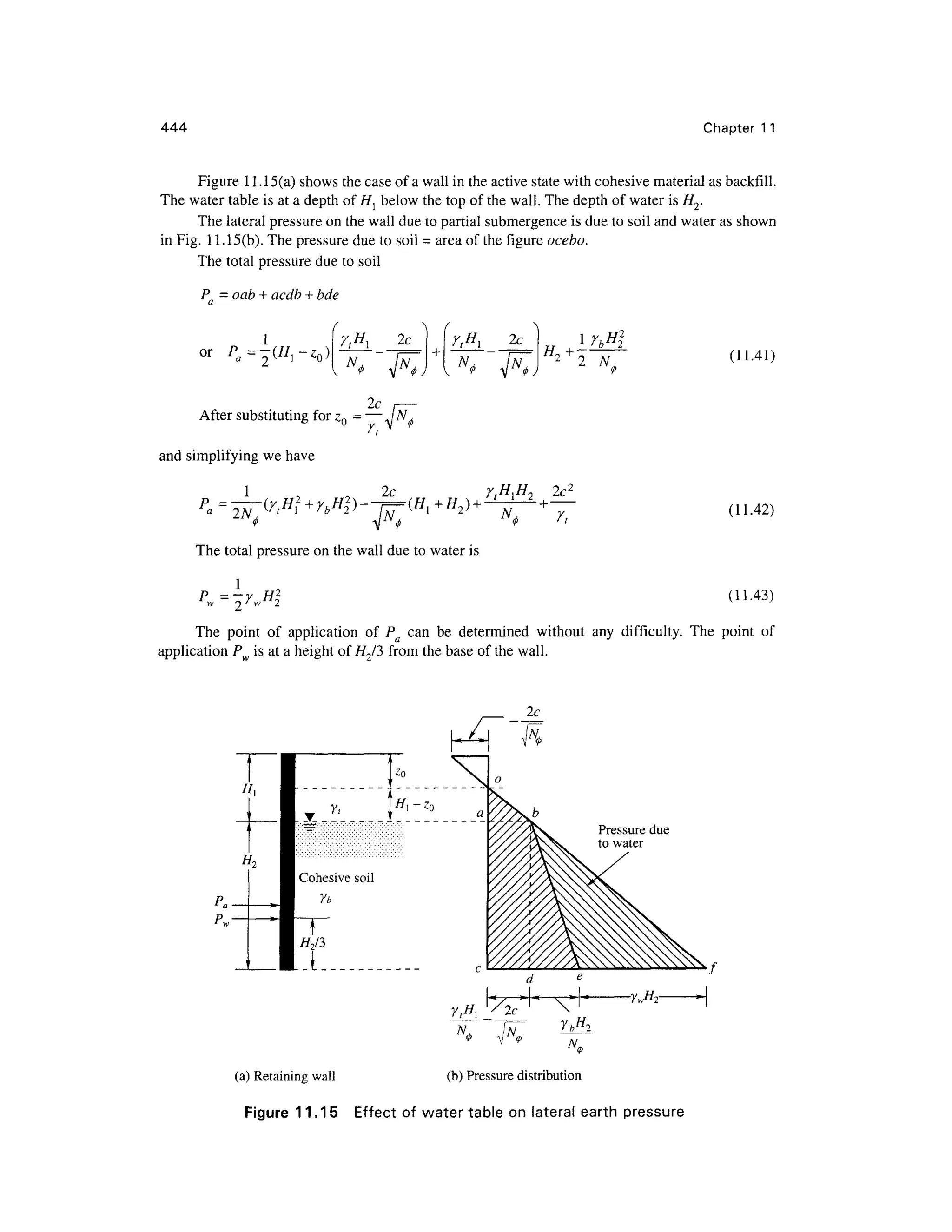
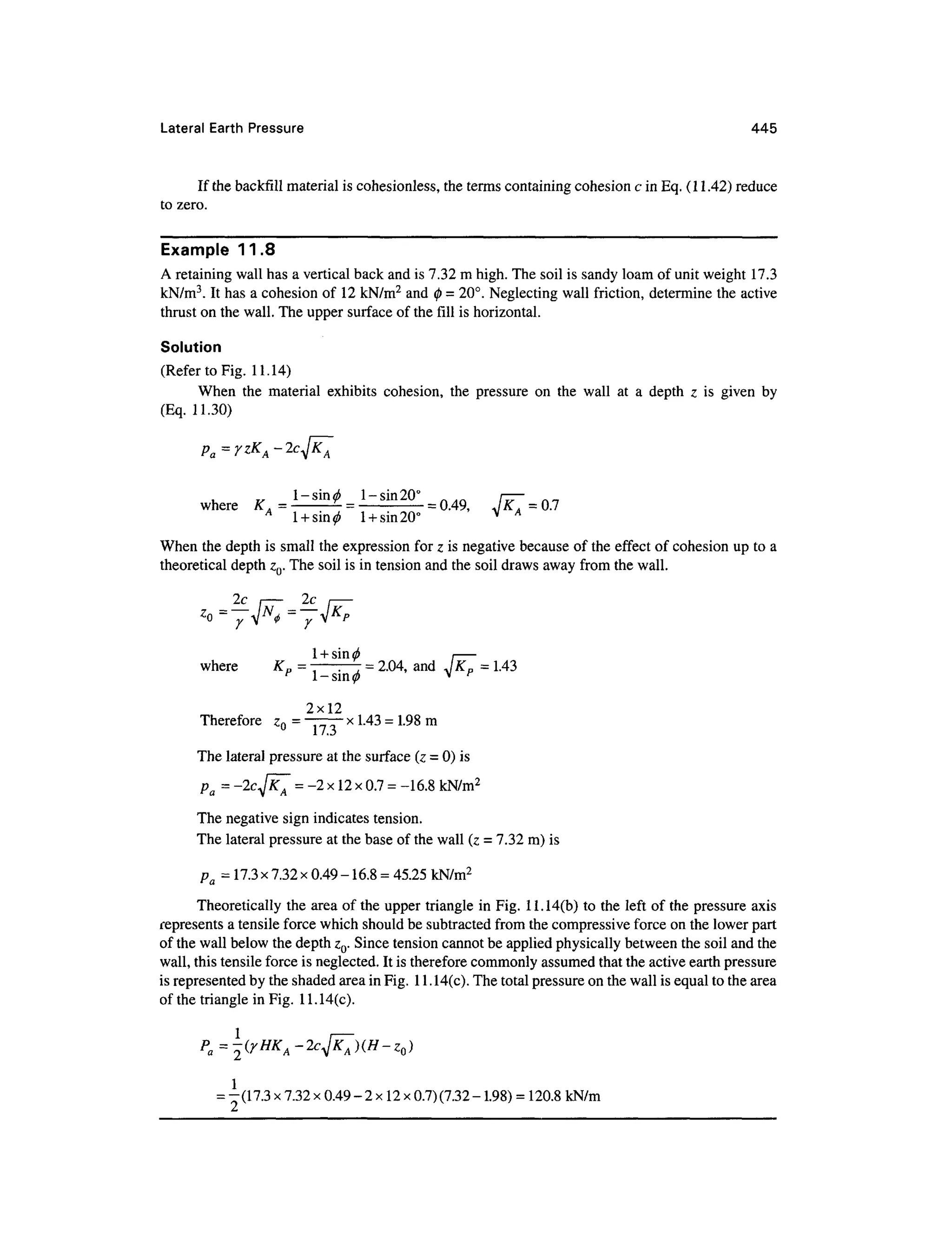
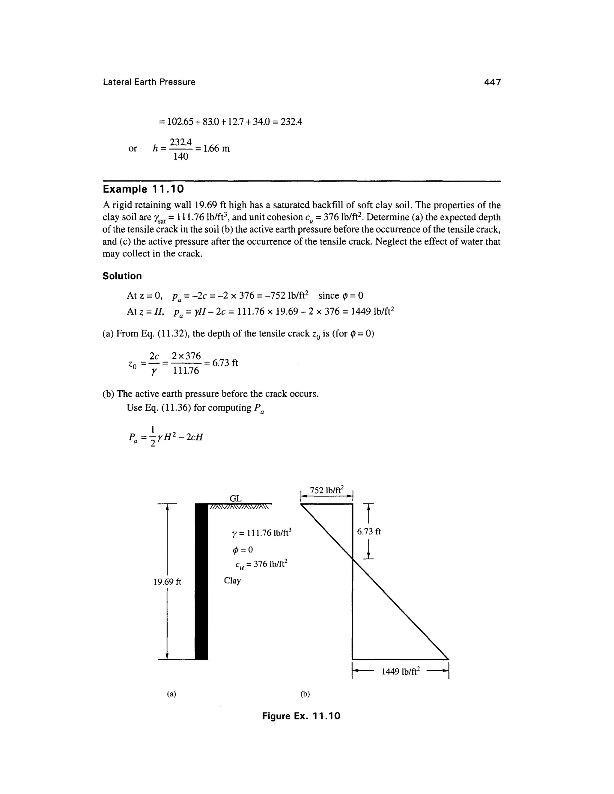
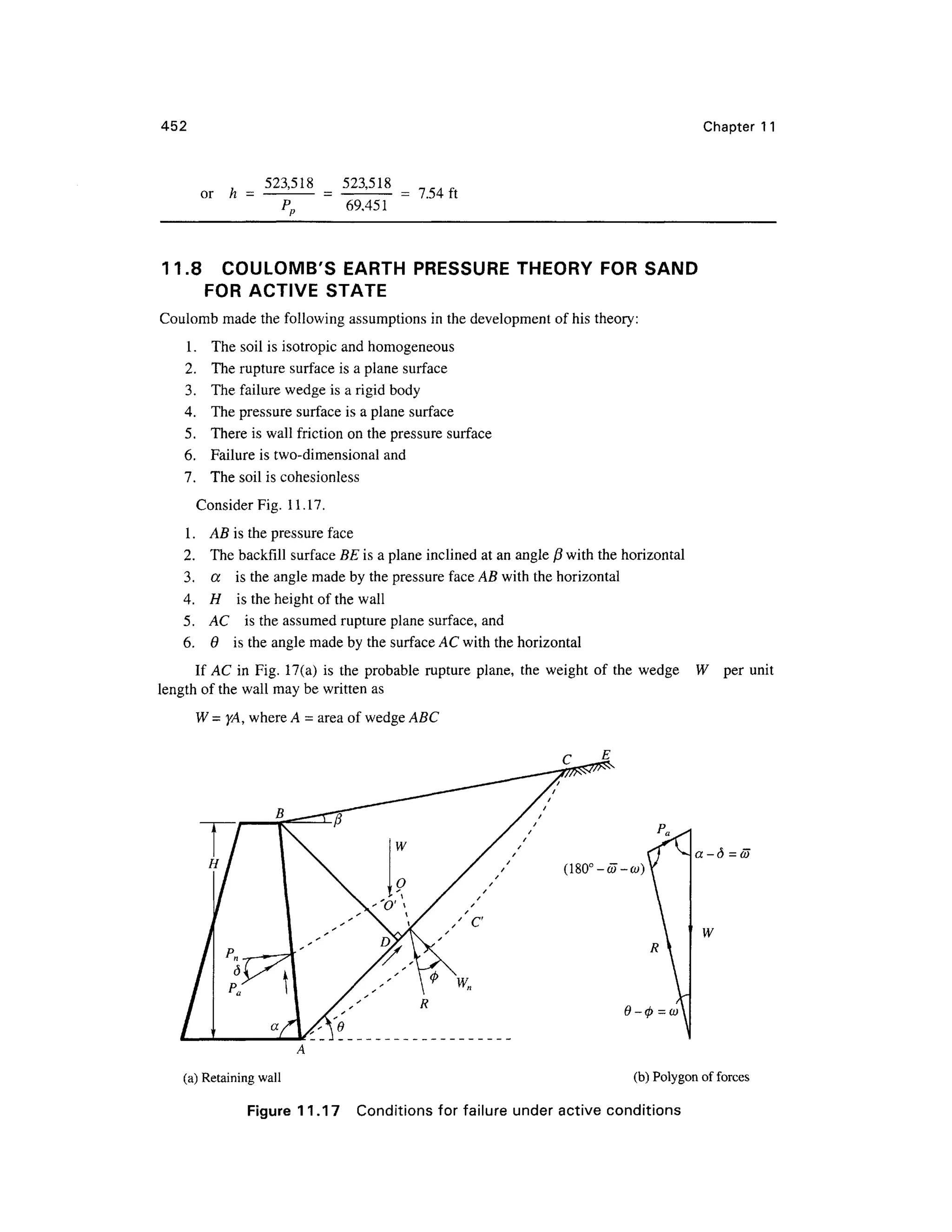
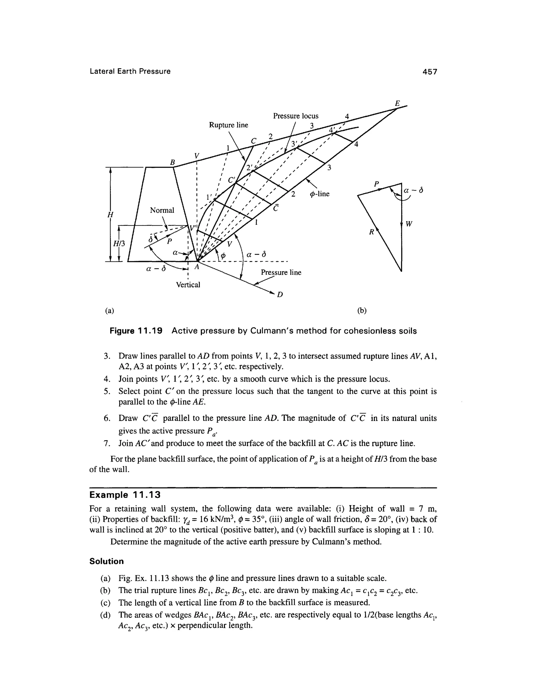
479. 460 Chapter 1 1
0.28Q n 2
H2
(0.1 6 + n2
)3 (11.65)
(c) Latera l pressur e a t point s alon g th e wal l o n eac h sid e o f a perpendicula r fro m th e
concentrated load Q to the wall (Fig. 11.20b )
Ph = Ph cos2
(l.la) (11.66)
Lateral Pressur e o n a Rigi d Wal l du e t o Lin e Loa d
A concrete block wall conduit laid on the surface, or wide strip loads may be considered a s a series of
parallel line loads as shown in Fig. 11.21 . The modified equations for computing ph ar e as follows:
(a) For m > 0.4
Ph= n H
(a) For m < 0.4
2x2 (11.67)
Ph =
0.203n
(0.16+ n2
)2 (11.68)
Lateral Pressur e o n a Rigi d Wal l du e t o Stri p Loa d
A stri p loa d i s a loa d intensit y with a finit e width , such a s a highway , railwa y lin e o r eart h
embankment which is parallel to the retaining structure. The application of load is as given in Fig.
11.22.
The equation for computing ph i s
ph = — (/?-sin/?cos2«r) (11.69a)
The tota l lateral pressure per uni t length of wall due to strip loading ma y b e expressed a s
(Jarquio, 1981 )
x = mH
*"] q/unit length
x
H
q/unit are a
Figure 11.2 1 Latera l pressure against a Figur e 11.22 Latera l pressure against a
rigid wall due to a line loa d rigi d wal l due to a strip load

480. Lateral Eart h Pressur e 461
(11.69b)
where a, = tan l
— an d cc~ = tan'
i H 2
A + B
Example 11.1 4
A railway line is laid parallel to a rigid retaining wall as shown in Fig. Ex. 11.14. The width of the
railway track and its distance from the wall is shown in the figure. The height of the wall is 10m.
Determine
(a) The unit pressure at a depth of 4m from the top of the wall due to the surcharge load
(b) Th e total pressure acting on the wall due to the surcharge load
Solution
(a)FromEq(11.69a)
The lateral earth pressure ph at depth 4 m is
2q
ph =—(/?-sin/?cos2a)
2x60 18.44
3.14 18 0
x 3.14 - sin 18.44° cos 2x36.9 = 8.92 kN/m2
(b)FromEq. (11.69b)
where, q = 60 kN/m2
, H = 10 m
2m . 2 m
»T*
= A
= B
Figure Ex . 11.14 "

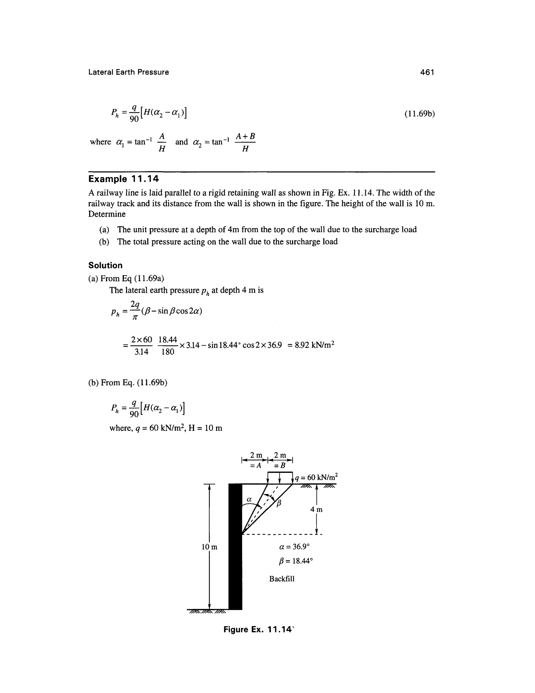
481. 462 Chapte r 1 1
, A
, 2
a, = tan"1
— = tan"1
— = 11.31°
H 1 0
T1
— ^tan" 1
—= 21.80 C
H 1 0
=—[10(21.80-11.31)] « 70 kN/m
11.12 CURVE D SURFACE S O F FAILURE FO R COMPUTING
PASSIVE EART H PRESSUR E
It is customary practice to use curved surfaces of failure for determining the passive earth pressur e
P o n a retaining wall with granular backfill if § is greater than 0/3. If tables or graphs are available
for determining K fo r curved surfaces of failure the passive earth pressure P ca n be calculated. If
tables or graphs are not available for this purpose, P ca n be calculated graphically by any one of
the following methods.
1 .Logarithmi c spira l method
2. Frictio n circle method
In bot h thes e methods , th e failur e surfac e clos e t o th e wal l i s assume d a s th e par t o f a
logarithmic spira l or a part of a circular arc with the top portion of the failure surfac e assumed as
planar. Thi s statemen t i s vali d fo r bot h cohesiv e an d cohesionles s materials . Th e method s ar e
applicable fo r bot h horizonta l an d incline d backfil l surfaces . However , i n th e followin g
investigations it will be assumed that the surface of the backfill i s horizontal.
Logarithmic Spira l Metho d o f Determinin g Passiv e Eart h Pressur e o f Idea l
Sand
Property o f a Logarithmi c Spira l
The equation of a logarithmic spiral may be expressed as
(11.70)
where
rQ = arbitrarily selected radius vector for reference
r = radius vector of any chosen point on the spiral making an angle 0 wit h rQ.
<j) = angle of internal friction o f the material .
In Fig. 11.23a O is the origi n o f the spiral . Th e propert y o f the spira l i s that every radius
vector suc h as Oa makes a n angle of 90°-0 to the tangent of the spiral at a or in other words, the
vector Oa makes an angle 0 with the normal to the tangent of the spiral at a.
Analysis o f Force s fo r th e Determinatio n o f Passiv e Pressur e P p
Fig. 1 1 .23b gives a section through the plane contact face AB of a rigid retaining wall which rotates
about poin t A int o the backfill o f cohesionless soi l wit h a horizontal surface. B D is drawn at an
angle 45°- 0/2 to the surface. Let Ol be an arbitrary point selected o n the line BD as the center of
a logarithmic spiral, and let O}A be the reference vecto r r Q. Assume a trial slidin g surface Aelcl
which consists of two parts. The first part is the curved part Ael which is the part of the logarithmic

482. Lateral Eart h Pressur e 463
0
Tangent
V,
(a) Properties of logarithmic spiral
Curve C
(c) Polygon of forces
-0/2 /
B
(b) Methods of analysis
Figure 11.23 Logarithmi c spiral method of obtaining passive earth pressure of sand
(After Terzaghi, 1943 )
spiral with center at Ol an d the second a straight portion elcl whic h is tangential to the spiral at
point e{ on the line BD.
e^c meets the horizontal surface at Cj at an angle 45°- 0/2. O
lel is the end vector rt of the
spiral which makes an angle 6l with the reference vector rQ . Line BD makes an angle 90°- 0 with
line ^Cj which satisfies the property of the spiral.
It is now necessary t o analyze the forces actin g on the soil mass lyin g above th e assumed
sliding surface A^jCj.
Within the mass of soil represented by triangle Belcl the state of stress is the same as that in
a semi-infinite mass in a passive Rankine state. The shearing stresse s along vertical section s ar e
zero in this triangular zone. Therefore, w e can replace the soil mass lying in the zone eldlcl b y a
passive earth pressure Pd acting on vertical section eldl a t a height hgl/3 wher e hg] i s the height of
the vertical section e{d{ . This pressure is equal to
p =
e (11.71)

483. 464 Chapte r 1 1
where W 0 = tan2
(45° + 0/2 )
The body of soil mass BAe]dl (Fig . 1 1.23b) is acted on by the following forces:
1. Th e weight Wj o f the soil mass acting through the center of gravity of the mass havin g a
lever arm /2 with respect to Or the center of the spiral.
2. Th e passive earth pressure /^acting on the vertical section el d} havin g a lever arm /3.
3. Th e passive earth pressure Pj acting on the surface AB at an angle S to the normal and at a
height H/3 abov e A having a lever arm l{ .
4. Th e resultant reaction forc e F l o n the curved surface Ae{ an d passing through the center
Determination o f th e Forc e />
1 Graphically
The directions of all the forces mentioned above except that of Fl ar e known. In order to determine
the direction o f F, combin e th e weight W { an d the force P el whic h gives th e resultant /?, (Fig .
1 1.23c). This resultant passes through the point of intersection nl of W{ and Pel i n Fig. 1 1.23b and
intersects forc e P { a t poin t n2. Equilibrium requires tha t forc e F { pas s throug h th e sam e point .
According t o th e propert y o f th e spiral , it mus t pass throug h th e sam e point . According t o th e
property of the spiral, it must pass through the center Ol o f the spiral also. Hence, the direction of
Fj is known and the polygon of forces shown in Fig. 1 1.23c can be completed. Thus we obtain the
intensity of the force P} require d to produce a slip along surface Aelcl .
Determination o f /* , b y Moment s
Force Pl ca n be calculated by taking moments of all the forces abou t the center O { o f th e spiral .
Equilibrium of the system requires that the sum of the moments o f all the forces mus t be equal to
zero. Since the direction of Fl i s now known and since it passes through Ol , it has no moment. The
sum of the moments o f all the other forces may be written as
P1 /1 +W1 /2 +J P1 /3 =0 (11.72 )
Therefore,P
=
-7(^2 + P
^) (11.73 )
l
i
Pl i s thus obtained fo r an assumed failure surface Ae^c^. The next step consists in repeating
the investigation for more tria l surfaces passing through A which intersect line BD at points e2, e3
etc. The values of Pr P 2 P 3 etc so obtained may be plotted as ordinates dl d{ , d2 d'2 etc., as shown
in Fig. 1 1 .23b and a smooth curve C is obtained by joining points d{ , d' 2 etc . Slip occurs along the
surface correspondin g t o th e minimu m value P whic h i s represente d b y th e ordinat e dd'. Th e
corresponding failur e surface is shown as Aec i n Fig. 1 1.23b.
11.13 COEFFICIENT S OF PASSIVE EARTH PRESSURE TABLES
AND GRAPH S
Concept o f Coulomb' s Formul a
Coulomb (1776 ) computed the passive earth pressure o f ideal sand on the simplifying assumptio n
that the entire surface of sliding consists of a plane through the lower edge A of contact face AB as
shown in Fig. 1 1.24a. Line AC represents a n arbitrary plane section throug h this lower edge. The
forces actin g on this wedge and the polygon of forces ar e shown in the figure. The basic equatio n
for computing the passive earth pressure coefficient ma y be developed a s follows:

484. Lateral Earth Pressure 465
Consider a point on pressure surface AB at a depth z from point B (Fig 11.24a) . The normal
component of the earth pressure per unit area of surface AB may be expressed by the equation,
Ppn = yzKp (11.74 )
where Kp i s the coefficient of passive earth pressure. The total passive earth pressure normal
to surface AB, P n, is obtained from Eq. (11.74) as follows,
zdz
sin asi n a
o o
pn
sm«
(11.75)
where a is the angle made by pressure surface AB with the horizontal.
Since the resultant passive earth pressure P act s at an angle 8 to the normal,
p = pn
- —
p
cos<5 2
K
s
sin cc cos o
(11.76)
H/3
(a) Principles of Coulomb's Theory of passive earth pressure of sand
30C
^ 20 °
"=3
<4-l
o
o i
35C
10 1 5
Values of K P
40C
20 25
(b) Coefficient of passive earth pressure K P
Figure 11.24 Diagra m illustrating passive earth pressure theory o f san d and
relation betwee n (j) , 8 and Kp (After Terzaghi, 1 943)

485. 466 Chapte r 1 1
Table 11. 3 Passiv e earth pressur e coefficient K' p for curve d surface s o f failur e
(After Caquo t an d Kerisel 1948).
0 =
3=0
(5=0/2
(5=0
8 = -0/2
10°
1.42
1.56
1.65
0.73
15°
1.70
1.98
2.19
0.64
20°
2.04
2.59
3.01
0.58
25°
2.56
3.46
4.29
0.55
30°
3.0
4.78
6.42
0.53
35°
3.70
6.88
10.20
0.53
40°
4.6
10.38
17.50
0.53
Eq. (11.76) may also be expressed a s
(11-77)
Kr,
where K' p = £— - (11.78 )
sin #cost)
Passive Eart h Pressur e Coefficien t
Coulomb develope d a n analytical solution for determining Kp base d on a plane surface of failure
and this is given in Eq. (11.57). Figure 11.24(b) gives curves for obtaining Coulomb's value s of K p
for various values of 8 and 0 for plane surfaces of failure with a horizontal backfill. They indicat e
that fo r a give n valu e o f 0 th e valu e of K p increase s rapidl y wit h increasin g value s o f 8 . The
limitations o f plan e surface s o f failur e ar e give n in Sectio n 11.9 . Curve d surface s o f failur e are
normally used for computing P o r Kp whe n the angle of wall friction 8 exceeds 0/3. Experienc e
indicates that the curved surface of failure may be taken either as a part of a logarithmic spiral or a
circular arc. Caquot an d Kerisel (1948 ) compute d K' p by making use of curved surfaces of failure
for various values of 0, 8, 0 and /3. Caquot and Kerisel's calculations for determining K' p for curved
surfaces of failure are available in th e form of graphs.
Table 11. 3 gives th e value s of K' pfor variou s values of 0 and 8 for a vertical wal l wit h a
horizontal backfill (after Caquot and Kerisel, 1948) .
In the vast majority of practical cases the angle of wall friction has a positive sign, that is, the
wall transmit s t o a soi l a downwar d shearin g force . Th e negativ e angl e o f wal l frictio n migh t
develop i n the case of positive batter piles subjecte d t o lateral loads , an d also in the case of pier
foundations for bridges subjecte d to lateral loads.
Example 11.1 5
A gravity retaining wall is 10 ft high with sand backfill. The backface of the wall is vertical. Given
8= 20°, and 0 = 40°, determin e the total passive thrust using Eq. (11.76) and Fig. 11.2 4 for a plane
failure. What is the passive thrust for a curved surface of failure? Assume y= 18. 5 kN/m3
.
Solution
From Eq. (11.76 )
1 K
P' = -Y H 2p
- wher e a = 90°
' 2 si n acos S
From Fig. 11.2 4 (b) for 8 = 20°, and 0 = 40°, we have Kp = 11

486. Lateral Earth Pressure 46 7
P = -xl8.5x!02
= 10,828 kN/m
p
2 si n 90 cos 20°
From Tabl e 11.3 K' p fo r a curved surface of failure (Caquot and Kerisel. 1948 ) for 0 = 40°
and 8 =20° is 10.38.
From Eq. (11.77)
p = -yH 2
K' = -x 18.5 x 102
x 10.38
p
2 p
2
= 9602kN/m
Comments
For S = $2, the reduction in the passive earth pressure due to a curved surface of failure is
10,828-9602
Reduction = — — x 100 =11.32%
Example 11.1 6
For th e dat a give n i n Exampl e 11.15 , determin e th e reductio n i n passiv e eart h pressur e fo r a
curved surface of failure if 8 = 30°.
Solution
For a plane surface of failure P fro m Eq. (11.76) is
P = -xl8.5x!02
x — = 22,431 kN/m
p
2 sin90°cos30 °
where, K = 21 from Fig. 11.24 for § = 30° and</ > = 40 °
From Table 11. 3 for 8 = 30° and</ » = 40°
K.f = 10.38 +17.50
From Eq(l 1.77)
P = -
x 18.5x!02
x 13.94 =12,895 kN/ m
p
2
o A .• • • 22,431-12,89 5 „„__ ,
Reduction i n passive pressure =
= 42.5%
22,431
It is clear fro m the abov e calculations , that the soil resistance unde r a passive stat e give s
highly erroneous values for plane surfaces of failure with an increase in the value of S. This erro r
could lead to an unsafe condition because the computed values of P woul d become highe r than
the actual soil resistance .
11.14 LATERA L EART H PRESSUR E O N RETAININ G WALL S
DURING EARTHQUAKE S
Ground motions durin g an earthquake tend t o increase th e earth pressur e abov e th e static eart h
pressure. Retaining walls with horizontal backfills designed with a factor of safety of 1.5 for static

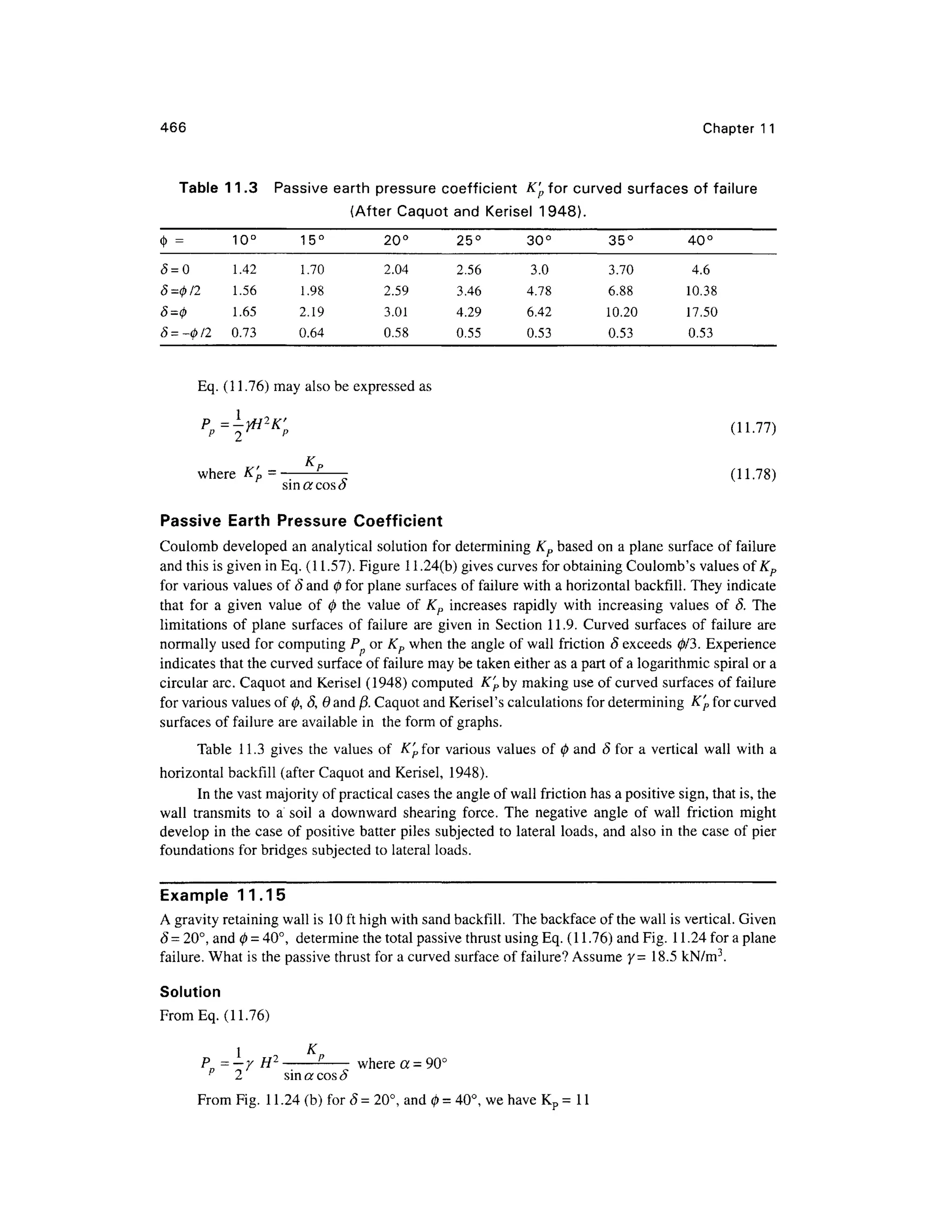
487. 468 Chapter 1 1
loading are expected t o withstand horizontal accelerations u p to 0.2g. For larger accelerations, and
for wall s with sloping backfill , additiona l allowances shoul d be made for the earthquake forces .
Murphy (1960) shows that when subjected to a horizontal acceleration a t the base, failure occurs in
the soil mass along a plane inclined at 35° from the horizontal . The analysis of Mononobe (1929 )
considers a soil wedge subjected to vertical and horizontal accelerations t o behave as a rigid body
sliding over a plane slip surface.
The current practice for earthquake design of retaining walls is generally based on design rules
suggested b y See d an d Whitman (1970). Richard s e t al. (1979) discus s the design an d behavior of
gravity retainin g wall s wit h unsaturate d cohesionless backfill. Most o f th e paper s mak e us e o f the
popular Mononobe-Okabe equations as a starting point for their own analysis. They follow generally the
pseudoplastic approac h fo r solving the problem. Solution s are available for both the active and passive
cases with as granular backfill materials. Though solutions for (c-0) soils have been presented by some
investigators (Prakas h an d Saran , 1966 , Saran and Prakash, 1968) , thei r findings have not yet been
confirmed, and as such the solutions for (c-0) soils have not been taken up in this chapter.
Earthquake Effec t o n Active Pressur e wit h Granula r Backfil l
The Mononobe-Okab e metho d (1929 , 1926 ) for dynamic lateral pressur e o n retaining walls is a
straight forward extensio n o f the Coulomb slidin g wedge theory. The forces tha t act on a wedge
under the active state are shown in Fig. 11.25
In Fig. 11.25 AC i n the slidin g surface o f failure of wedg e ABC havin g a weigh t W with
inertial components k v W and khW. The equation for the total active thrust Pae acting on the wall AB
under dynamic force conditions as per the analysis of Mononobe-Okabe i s
(11.79)
in which
K. = •
Ae
cos //cos2
<9cos(#+ 0+77) 1+
cos( 8+ 9+ /7)cos(/?- 9]
(11.80)
Figure 11.2 5 Activ e forc e on a retaining wal l with earthquake force s

488. Lateral Earth Pressure 469
where P ae =dynamic component of the total earth pressure P ae o r Pae = Pa + Pae
KAe = the dynamic earth pressure coefficient
77 = tan" (11.81)
Pa = active earth pressure [Eq . (11.50)]
kh = (horizontal acceleration)/g
kv ^(vertical acceleration)/g
g = acceleration due to gravity
y= unit weight of soil
0 = angle of friction of soil
8 = angle of wall friction
/3 =slope of backfill
6 = slop e o f pressur e surfac e o f retainin g wal l wit h respec t t o vertica l a t poin t B
(Fig. 11.25 )
H = height of wall
The total resultant active earth pressure Pae due to an earthquake is expressed as
P - P +P
L
ae L
a ^ l
ae (11.82)
The dynamic component P ae is expected to act at a height 0.6H abov e the base whereas the
static earth pressure acts at a height H/3. For all practical purposes it would be sufficient to assume
that the resultant force Pae acts at a height H/2 above the base with a uniformly distributed pressure.
0.7
0.6
0.5
50.4
c
0.2
0.1
= 0,0 = 0,0 =
= 1/2 0
'0 = 30C
'0 = 35<
0 0. 1 0. 2 0. 3 0. 4 0. 5
kh
(a) Influence of soil frictio n
on soil dynamic pressure
u. /
n f
O c
"O n A
T3
C
v? A a
O 9
0 1
A
°(
//,
^x
) 0
0
/
/
//
X
1 0
= 20°
/ ft
A
//
/ s
2 0
/
= 10°
ft =
/=
kv-0
d = l
/2
3 0
/
°v
-10°
:o
6> - 0
0
4 0 .
(b) Influence of backfill slop e on
dynamic lateral pressure
Figure 11.26 Dynami c latera l active pressur e (after Richards et al., 1979 )

489. 470 Chapter 1 1
It has been show n that the active pressure i s highly sensitive to both the backfill slope (3, and th e
friction angl e 0 of the soil (Fig. 11.26) .
It is necessary t o recognize the significance of the expressio n
(11.83)
given under the root sign in Eq. (11.80).
a. Whe n Eq. (1 1.83) is negative no real solution is possible. Henc e fo r stability, the limiting
slope of the backfill mus t fulfill th e condition
P<(tp-ri)
b. Fo r no earthquake condition, r| = 0. Therefore fo r stability we have
p<q>
c. Whe n the backfill i s horizontal (3 = 0. For stability we have
ri<(p
d. B y combining Eqs. (1 1.81) and (1 1.86), we have
(11.84a)
(11.85)
(11.86)
(11.87a)
From Eq. ( 1 1.87a), we can define a critical value for horizontal acceleration k* h a s
^=(l-fcv )tan^ (11.87b )
Values of critical accelerations ar e given in Fig 11.2 7 which demonstrates th e sensitivity of
the various quantities involved.
0.7
0.6
0.5
0.2
0.1
10 2 0 3 0 4 0
0 degrees
Figure 11.2 7 Critica l value s of horizonta l acceleration s

490. Lateral Eart h Pressure 47 1
Effect o f Wal l Latera l Displacemen t o n the Desig n of Retainin g Wall
It is the usual practice of some designers to ignore the inertia forces of the mass of the gravity
retaining wal l i n seismi c design . Richard s an d Elm s (1979 ) hav e show n tha t thi s approac h i s
unconservative since it is the weight of the wall which provides most of the resistance t o lateral
movement. Taking into account all the seismic forces acting on the wall and at the base they have
developed a n expression fo r th e weigh t of the wal l Ww under the equilibriu m condition as (for
failing by sliding)
Ww=±yH2
(l-kv)KAeCIE (11.88 )
in which,
cos(S +6>) - sin(£ +6>) tan S
1E
(l-& v)(tan£-tan77) (11.89 )
where W w= weight of retaining wall (Fig. 11.25 )
8
= angle of friction between the wall and soil
Eq. (11.89) is considerably affected by 8. If the wall inertia factor is neglected, a designer will
have to go to an exorbitant expense to design gravity walls.
It is clear that tolerable displacement of gravity walls has to be considered i n the design. The
weight of the retaining wall is therefore required to be determined to limit the displacement to the
tolerable limit. The procedure is as follows
1. Se t the tolerable displacement Ad
2. Determin e the design value of kh by making use of the following equation (Richards et al., 1979)
0.2 A,2
^
where Aa, AV = acceleration coefficients used in the Applied Technology Counci l (ATC) Building
Code (1978) for various regions of the United States. M is in inches.
3. Usin g the values of kh calculated above, and assuming kv - 0 , calculate KAe from Eq (11.80)
4. Usin g the value of KAe, calculate the weight, Ww, of the retaining wall by making use of
Eqs. (11.88) and (11.89)
5. Appl y a suitable factor of safety, say, 1.5 to Ww.
Passive Pressur e Durin g Earthquake s
Eq. (11.79 ) gives a n expression fo r computing seismic activ e thrust which is based o n the well
known Mononobe-Okabe analysi s for a plane surface of failure. The corresponding expression for
passive resistance is
Ppe=2
^-k
^K
Pe (11.91 )
KPe= —
cosrjcos2
0cos(S-0+Tj) 1- .

491. 472 Chapter 1 1
Figure 11.2 8 Passiv e pressure on a retaining wal l during earthquake
Fig. 11.2 8 gives the various forces acting on the wall under seismic conditions. All the other
notations in Fig. 11.2 8 are the same as those in Fig. 11.25 . The effect o f increasing the slope angle
P is to increase the passive resistance (Fig. 11.29). The influence of the friction angle of the soil (0)
on the passive resistance is illustrated the Fig. 11.30 .
Figure 11.2 9 Influenc e o f backfil l slope angle on passive pressure

492. Lateral Eart h Pressure 473
0 0. 2 0. 4 0. 6
Figure 11.30 Influenc e o f soil friction angle on passive pressure
It ha s bee n explaine d i n earlie r section s o f thi s chapte r tha t th e passiv e eart h pressure s
calculated on the basis of a plane surface of failure give unsafe results if the magnitude of 6 exceeds
0/2. The erro r occur s becaus e th e actua l failure plane i s curved , with th e degre e o f curvatur e
increasing wit h an increas e i n th e wal l frictio n angle . The dynami c Mononobe-Okabe solutio n
assumes a linear failure surface, as does the static Coulomb formulation.
In order to set right this anomaly Morrison and Ebelling (1995) assumed the failure surface as
an arc of a logarithmic spira l (Fig . 11.31 ) and calculated th e magnitud e of the passive pressur e
under seismic conditions.
It i s assume d her e tha t th e pressur e surfac e i s vertica l (9= 0) an d th e backfil l surfac e
horizontal (j3 =0). The following charts have been presented by Morrison and Ebelling on the basis
of their analysis.
Logarithmic spira l
Figure 11.31 Passiv e pressure from lo g spiral failure surface during earthquake s

493. 474 Chapter 1 1
LEGEND
Mononobe-Okabe
Log spiral
0 0.1 0 0.2 0 0.3 0 0.4 0 0.5 0 0.6 0
Figure 11.3 2 K pe versu s kh, effect o f 8
LEGEND
Mononobe-Okabe
Log spiral
kv = 0,6= (2/3)0
0.60
Figure 1 1.33 K pe versus kh, effect of
1 . Fig . 1 1 .32 gives the effect o f 5 on the plot Kpe versu s kh with kv = 0, for 0 =30°. The values
of § assumed are 0, 1/ 2 (())) and(2/3<j)) . The plo t shows clearly th e difference between th e
Mononobe-Okabe an d lo g spira l values. The differenc e betwee n the tw o approache s i s
greatest at kh = 0

494. Lateral Earth Pressur e 47 5
2. Fig . 11.33 show s th e effec t o f 0 o n K pg. Th e figur e show s th e differenc e betwee n
Mononobe-Okabe and log spiral values of K versu s kh with 8=( 2/30) and kv = 0. It is also
clear from the figure the difference between the two approaches is greatest for kh - 0 and
decreases with an increase in the value of kh.
Example 11.1 7
A gravity retaining wall is required to be designed for seismic conditions for the active state. The
following data are given:
Height of wall =8 m 0= 0° , 0=0, 0=30°, &= 15°, £, =0, kh = 0.25 and y=19kN/m3
. Determine
Pae and the approximate point of application. What is the additional activ e pressure caused b y th e
earthquake?
Solution
From Eq. (11.79)
Pae=rH2
(l-kv)KAe=^yH^KAe, sinc e *y = 0
For 0 = 30°, 5= 15° and kh = 0.25, we have from Fig. 11.26 a
KAe = 0.5. Therefore
pag = -?-19x82
x 0.5 =304 kN/m
1 9
From Eq. (11.14) P a= -y H 2
KA
2
° -2
where K A = tan2
(45° - ^ 2) = tan2
30° =0.33
Therefore P a = - x 19 x 82
x0.33 = 202.7 kN/m
&Pae = the additional pressure du e to the earthquake = 304 -202. 7 = 101.3 kN/m
For all practical purposes, the point of application of Pae may be taken as equal to H/2 above
the base of the wall or 4 m above the base in this case.
Example 11.1 8
For th e wal l give n i n Exampl e 11.17 , determin e th e tota l passiv e pressur e P e unde r seismi c
conditions. What is the additional pressure due to the earthquake?
Solution
From Eq. (11.91),
Pae = rH*(l-k v)Kpe = 7H*K pe, sinc e *v =0
From Fig 1 1.32, (from M-O curves), Kpe = 4.25 for 0 = 30°, and 8= 15°
Now/3
= -/H 2
K= -x!9x8 2
x 4.25 = 2584 kN/ m
pe 2 P e
9

495. 476 Chapter 1 1
FromEq. (11.15 )
p = -7H2
K = - x ! 9 x 8 2
x 3 =
p
2 p
2
30
where # = tan2
45° + — | = tan2
60° =3
= (P
pe - P
Pe) = 2584
~ 182
4 =76
° k
N
/
11.15 PROBLEM S
11.1 Fig . Prob. 11.1 shows a rigid retaining wall prevented fro m lateral movements . Determin e
for thi s wall the lateral thrus t for the at-rest conditio n an d the point of application o f the
resultant force .
11.2 Fo r Prob 11.1, determine the active earth pressure distributio n for the following cases :
(a) when the water table i s below the base and 7= 17 kN/rn3
.
(b) when the water table is at 3m below ground level
(c) when the water table is at ground level
11.3 Fig . Prob . 11. 3 gives a cantilever retaining wall with a sand backfill. The properties o f the
sand are :
e = 0.56, 0 = 38°, and G^ = 2.65.
Using Rankin e theory , determin e th e pressur e distributio n wit h respec t t o depth , th e
magnitude and the point of application of the resultant active pressure wit h the surcharg e
load bein g considered .
Ground surface
.:''. .'•: ..'Sand •:'.'•.*•/ .
3 m . ' . ' - ' ' ' " " ' ,
:•••.•• :y=1 7 kN/m3
-..'• .-.•..'• : ..'Sand •''.•':.:'
4.5m V ;
'.';
' :•".' ' '- .
./ y sat
= 19.8kN/m3
:•.'•••'••
= 34 °
Surcharge, q = 500 lb/ft2
1 1 1
Saturated sand
= 0.56
= 38° G s =2.65
Figure Prob. 11.1 Figure Prob . 11.3

496. Lateral Eart h Pressure 477
11.4 A smooth vertical wall 3.5m high retains a mass of dry loose sand. The dry unit weight of
the sand is 15.6 kN/m3
and an angle of internal friction 0is 32°. Estimate the total thrust per
meter acting against the wall (a) if the wall is prevented from yielding, and (b) if the wall is
allowed to yield.
11.5 A wall of 6 m height retains a non-cohesive backfill of dry unit weight 1 8 kN/m3
and an
angle of internal friction o f 30°. Use Rankine's theory and find the total active thrust per
meter lengt h o f th e wall . Estimat e th e chang e i n th e tota l pressur e i n th e following
circumstances:
(i) Th e top of the backfill carrying a uniformly distributed load of 6 kN/m2
(ii) Th e backfill under a submerged condition with the water table at an elevation of 2 m
below the top of the wall. Assume Gs -2.65 , and the soil above the water table being
saturated.
11.6 Fo r the cantilever retaining wall given in Fig. Prob 11. 3 with a sand backfill, determin e
pressure distribution with respect to depth and the resultant thrust. Given:
Hl = 3m, H2 = 6m, ysat = 19.5 kN/m3
q =25 kN/m2
, and 0= 36 °
Assume the soil above the GWT is saturated
11.7 A retaining wall of 6 m height having a smooth back retains a backfill made up of two strata
shown in Fig . Prob . 11.7 . Construc t the activ e eart h pressur e diagra m and fin d the
magnitude and point of application of the resultant thrust. Assume the backfill above WT
remains dry.
11.8 (a ) Calculate the total active thrust on a vertical wall 5 m high retaining sand of unit weight
17 kN/m3
for which 0 = 35°. The surfac e is horizontal an d the water table i s below th e
bottom of the wall, (b) Determine the thrust on the wall if the water table rises to a level 2 m
below the surface of the sand. The saturated unit weight of the sand is 20 kN/m3
.
11.9 Figur e Problem 11. 9 shows a retaining wall with a sloping backfill. Determine the active
earth pressure distribution, the magnitude and the point of application of the resultant by
the analytical method.
Cinder
H,-2m £. = «
•
XVVVvXX/'WVS
Figure Prob. 11. 7 Figure Prob . 11. 9

497. 478 Chapter 1 1
j |
j g =50kN/m:
A ~ ~
Soil A 6 m H l
• SO U t i I i
Figure Prob . 11.1 0
11.10 Th e soi l condition s adjacen t to a rigid retaining wall ar e show n i n Fig . Prob . 11.10 , A
surcharge pressure of 50 kN/m2
is carried on the surface behind the wall. For soil (A) above
the water table, c'= 0, 0' =38°, y' =18 kN/m3
. For soil (B) below the WT, c'= 1 0 kN/m2
,
0'= 28°, and ysat = 20 kN/m3
. Calculate the maximum unit active pressure behind the wall,
and the resultant thrust per unit length of the wall.
11.11 Fo r the retaining wall given in Fig. Prob. 11.10 , assume the following data:
(a) surcharg e load = 100 0 lb/ft 2
, and (b) Hl = 10 ft, H2 = 20 ft,
(c) Soi l A: c'= 50 0 lb/ft2
, 0' = 30°, y =110 lb/ft3
(d) Soi l B: c'= 0 , 0'= 35°, y sat = 120 lb/ft3
Required:
(a) Th e maximum active pressure at the base of the wall.
(b) Th e resultant thrust per unit length of wall.
11.12 Th e depth s o f soi l behin d an d i n fron t o f a rigi d retainin g wal l ar e 2 5 f t an d 1 0 f t
respectively, bot h th e soi l surface s bein g horizonta l (Fig . Pro b 11.12) . The appropriat e
'A //A //
0 = 22°
c = 600 lb/ft2
y =110 lb/ft 3
Figure Prob. 11.12

498. Lateral Eart h Pressur e 479
shear strengt h parameters fo r the soil are c = 600 lb/ft2
, an d 0 = 22°, and the unit weight
is 110 lb/ft3
. Using Rankine theory, determine the total active thrust behind the wall and the
total passive resistance i n front of the wall. Assume the water table is at a great depth.
11.13 Fo r the retaining wall given in Fig. Prob. 11.12 , assume the water table is at a depth of 10 ft
below the backfill surface. The saturated unit weight of the soil is 120 lb/ft3
. The soil above
the GWT is also saturated. Compute the resultant active and passive thrusts per unit length
of the wall.
11.14 A retaining wall has a vertical back face and is 8 m high. The backfill has the following
properties:
cohesion c = 15 kN/m2
, 0 = 25°, y =18.5 kN/m 3
The wate r tabl e i s a t grea t depth . The backfill surfac e i s horizontal. Dra w th e pressur e
distribution diagra m an d determin e th e magnitud e an d th e poin t o f applicatio n o f th e
resultant active thrust .
11.15 Fo r the retaining wall given in Prob. 11.14 , the water table is at a depth of 3 m below the
backfill surface. Determine the magnitude of the resultant active thrust.
11.16 Fo r the retaining wall given in Prob. 11.15, compute the magnitude of the resultant active
thrust, if the backfill surface carries a surcharge load of 30 kN/m2
.
11.17 A smooth retaining wall is 4 m high and supports a cohesive backfill with a unit weight of
17 kN/m3
. The shear strengt h parameters o f the soil ar e cohesion = 1 0 kPa and 0 = 10° .
Calculate the total active thrust acting against the wall and the depth to the point of zero
lateral pressure .
11.18 A rigid retaining wall is subjected to passive earth pressure. Determin e th e passive eart h
pressure distribution and the magnitude and point of application o f the resultant thrust by
Rankine theory.
Given: Heigh t o f wal l = 1 0 m ; dept h o f wate r tabl e fro m groun d surfac e = 3 m ;
c - 2 0 kN/m2
, 0 = 20° and ysat = 19. 5 kN/m3
. The backfill carries a uniform surcharge of
20 kN/m2
.
Assume the soil above the water table is saturated.
11.19 Fig . Prob. 11.19 gives a retaining wall with a vertical back face and a sloping backfill . All
the other data are given in the figure. Determine the magnitude an d point of application of
resultant active thrust by the Culmann method.
y =115 lb/ft 3
0 = 38
°
d = 25°
Figure Prob . 11.1 9

499. 480 Chapter 1 1
6 ft **
- 8f t — |
q= 12001b/ft 2
5ft
25ft
Figure Prob. 11.20
11.20 Fig . Prob. 11.20 gives a rigid retaining wall with a horizontal backfill. The backfill carries
a strip load of 120 0 lb/ft 2
a s shown in the figure. Determine the following:
(a) Th e uni t pressure o n the wal l at poin t A at a depth o f 5 ft below th e surfac e du e t o th e
surcharge load .
(b) Th e total thrust on the wall due to surcharge load.
11.21 A gravity retaining wall with a vertical back face is 1 0 m high . The followin g dat a ar e
given:
0=25°, S= 15°, and y= 19kN/m 3
Determine th e total passive thrus t using Eq (11.76). What is the total passive thrus t for a
curved surface of failure?
11.22 A gravit y retaining wall is required t o b e designed fo r seismi c condition s fo r th e activ e
state. The back face is vertical. The following data are given:
Height of wall = 30 ft, backfill surface is horizontal; 0 = 40°, 8 = 20°, kv = 0, kh = 0.3, y =
120 lb/ft 3
.
Determine th e total active thrust on the wall. What is the additional lateral pressure due to
the earthquake?
11.23 Fo r the wall given in Prob 11.22 , determine the total passive thrust during the earthquake
What is the change in passive thrust due to the earthquake? Assume $ = 30° and 8 = 15°.

500. CHAPTER 12
SHALLOW FOUNDATIO N I :
ULTIMATE BEARIN G CAPACIT Y
12.1 INTRODUCTIO N
It is the customary practice to regard a foundation as shallow if the depth of the foundation is less
than or equal to the width of the foundation. The different types of footings that we normally come
across ar e give n i n Fig. 12.1 . A foundation is a n integral part o f a structure. The stabilit y of a
structure depends upo n the stability of the supportin g soil. Two important factor s tha t are to be
considered ar e
1. Th e foundation must be stable against shear failure of the supporting soil.
2. Th e foundation must not settle beyond a tolerable limit to avoid damage to the structure.
The other factors that require consideration are the location and depth of the foundation. In
deciding the location and depth, one has to consider the erosions due to flowing water, underground
defects such as root holes, cavities, unconsolidated fills, ground water level, presence of expansive
soils etc.
In selecting a type of foundation, one has to consider the functions of the structure and the
load it has to carry, the subsurface condition of the soil, and the cost of the superstructure.
Design load s als o pla y a n importan t part i n th e selectio n o f th e typ e o f foundation . The
various load s tha t ar e likel y t o b e considere d ar e (i ) dead loads , (ii ) live loads , (iii ) wind and
earthquake forces, (iv) lateral pressures exerted by the foundation earth on the embedded structural
elements, and (v) the effects o f dynamic loads.
In additio n t o th e abov e loads , th e load s tha t ar e du e t o th e subsoi l condition s ar e als o
required t o be considered. They ar e (i) lateral o r uplift force s on the foundation elements du e to
high water table, (ii) swelling pressures on the foundations in expansive soils, (iii) heave pressures
481

501. 482 Chapter 1 2
(c) (d)
Figure 12. 1 Type s of shallo w foundations : (a) plain concrete foundation,
(b) steppe d reinforce d concrete foundation, (c ) reinforced concrete rectangula r
foundation, and (d) reinforced concrete wall foundation .
on foundations in areas subjected to frost heave and (iv) negative frictional drag on piles where pile
foundations are used in highly compressible soils .
Steps for th e Selectio n o f th e Typ e o f Foundatio n
In choosing the type of foundation, the design engineer must perform five successive steps .
1. Obtai n the required information concerning the nature of the superstructure and the load s
to be transmitted to the foundation.
2. Obtai n the subsurface soil conditions.
3. Explor e th e possibilit y o f constructin g any on e o f th e type s o f foundatio n under th e
existing conditions by taking into account (i) the bearing capacity of the soil to carry the
required load, an d (ii) the adverse effects o n the structure due to differential settlements.
Eliminate in this way, the unsuitable types.
4. Onc e one or two types of foundation are selected on the basis of preliminary studies, make
more detaile d studies . These studies may require mor e accurat e determinatio n o f loads ,
subsurface condition s and footing sizes. It may als o b e necessary t o make more refined
estimates of settlement in order to predict the behavior of the structure.

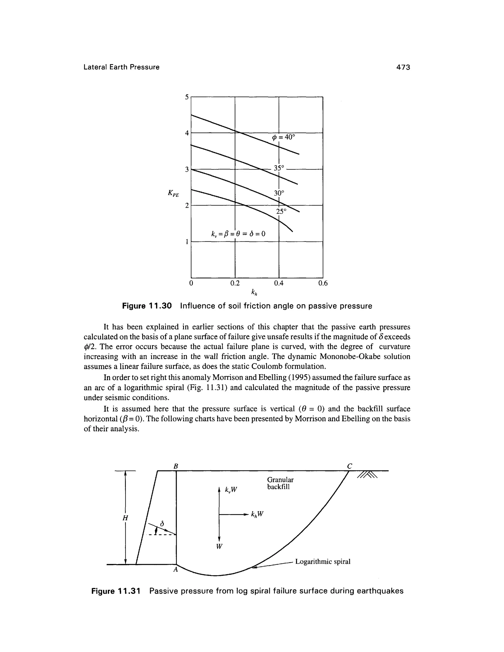
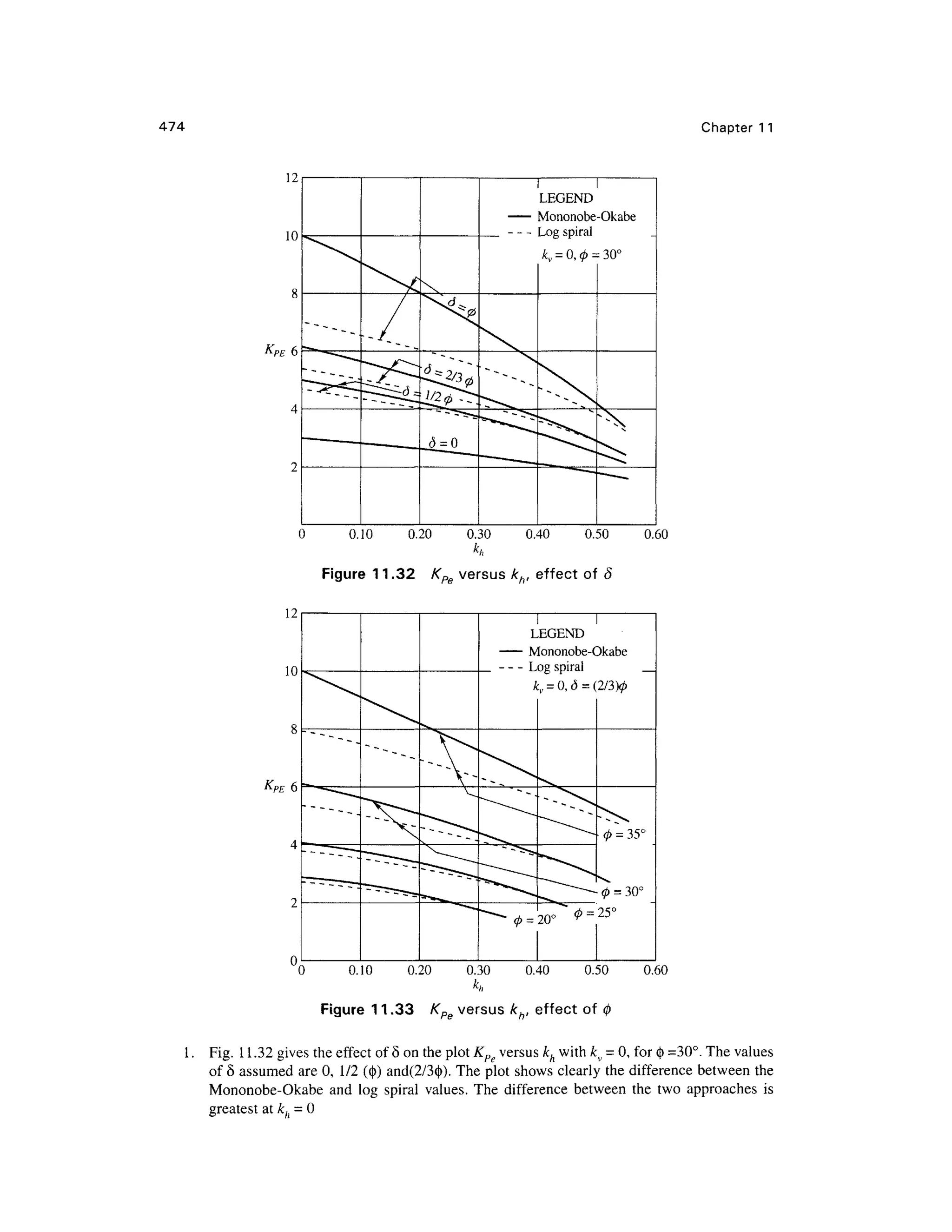
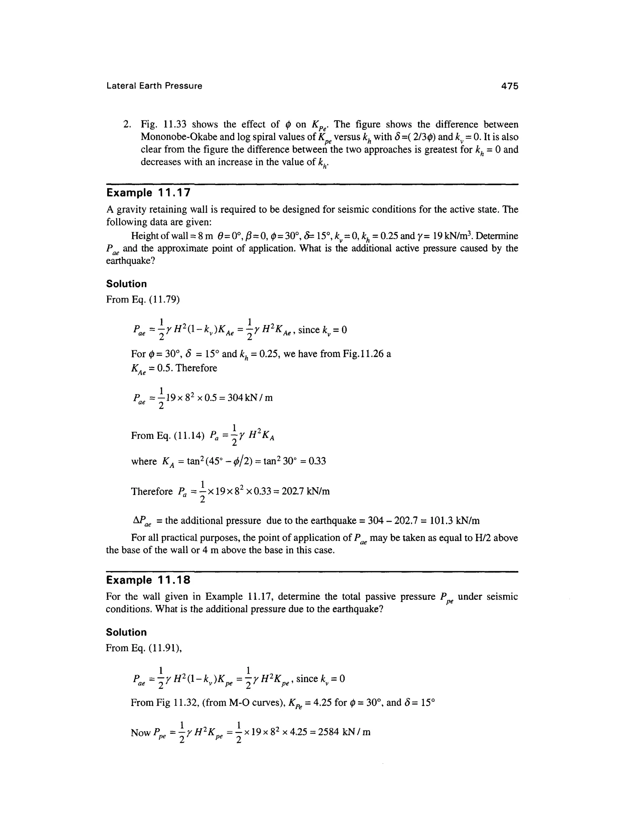
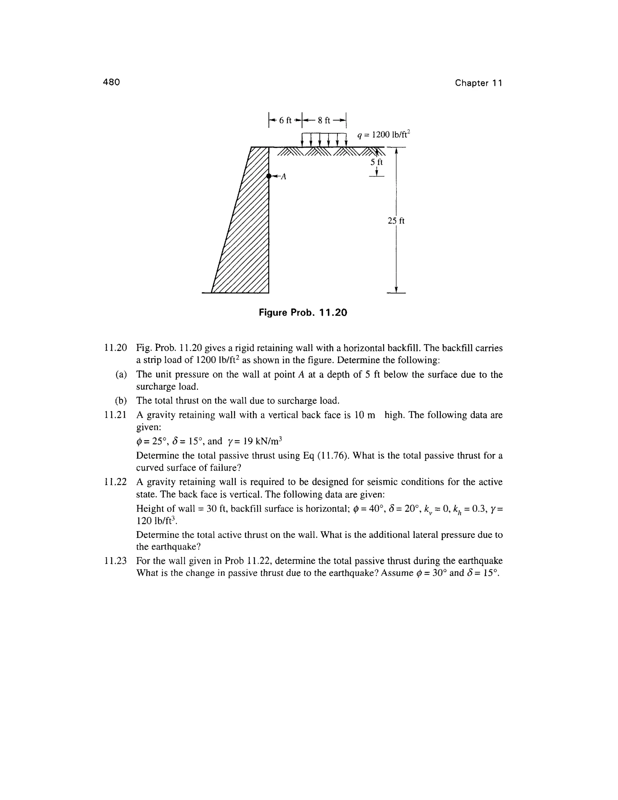
502. Shallow Foundatio n I: Ultimate Bearin g Capacit y 483
5. Estimat e the cost of each of the promising types of foundation, and choose th e type that
represents the most acceptable compromise between performance and cost.
12.2 TH E ULTIMAT E BEARIN G CAPACITY O F SOIL
Consider the simplest case of a shallow foundation subjected to a central vertical load. The footing
is founded at a depth Df below the ground surface [Fig. 12.2(a)] . If the settlement, 5, of the footing
is recorded against the applied load, Q, load-settlement curves, similar in shape to a stress-strain
curve, may be obtained as shown in Fig. 12.2(b) .
The shap e o f th e curv e depend s generall y o n th e siz e an d shap e o f th e footing , th e
composition o f the supporting soil, and the character, rate, and frequency o f loading. Normally a
curve will indicate the ultimate load Qu that the foundation can support. If the foundation soil is a
dense sand or a very stiff clay, the curve passes fairly abruptly to a peak value and then drops down
as shown by curve Cl in Fig. 10.2(b) . The peak load Q u is quite pronounced in this case. On the
other hand, if the soil is loose sand or soft clay, the settlement curve continues to descend on a slope
as show n by curv e C 2 whic h show s tha t the compressio n o f soi l i s continuousl y takin g plac e
without giving a definite value for Qu. On such a curve, Qu may be taken at a point beyond which
there is a constant rate of penetration.
12.3 SOM E O F THE TERMS DEFINE D
It will be useful to define, at this stage, some of the terms relating to bearing capacity of foundations
(refer to Fig. 12.3) .
(a) Tota l Overburden Pressur e q0
qo is the intensity of total overburden pressure due to the weight of both soil and water at the base
level of the foundation.
a — vD+ v D {"191 1
^n I U
MU ~ I int^w i
^-i
).
Q
L
Quit Load
(a) Footing (b ) Load-settlement curve s
Figure 12. 2 Typica l load-settlemen t curve s

503. 484 Chapter 1 2
Df
GL
/ZXSs/^X^
GWT
V
v^-XvX-X-
III
,
'
Qu,,
^
15.1
GL
7
/sat
<?'o
in
(Df-Dwl) = Dw, y - uni t weight of soil above GWT
ysat = saturated uni t weight of soil below GWT
Vb =
(/sat ~ 7w> - submerge d uni t weight of soil
yw = unit weight of water
Figure 12.3 Tota l an d effective overburde n pressure s
(b) Effectiv e Overburden Pressure qr' 0
<?« is the effective overburden pressur e a t the base level of the foundation .
when O,q 'Q = yDw{= yDf .
(12.2)
(c) Th e Ultimat e Bearin g Capacity of Soil, qu
qu is the maximum bearing capacity of soil at which the soil fails by shear .
(d) Th e Ne t Ultimat e Bearin g Capacity, qnu
qnu is the bearing capacity in excess of the effective overburden pressure q' Q, expressed a s
(e) Gross Allowable Bearin g Pressure, qa
qa is expressed a s
3a-jr
where Fs = factor of safety.
(f) Ne t Allowabl e Bearin g Pressure, qna
q i s expressed a s
(12.3)
(12.4)
_qnu
(12.5)

504. Shallow Foundation I: Ultimate Bearin g Capacity 485
(g) Saf e Bearing Pressure, qs
qs is defined as the net safe bearing pressure which produces a settlement of the foundation which
does not exceed a permissible limit.
Note: In the design of foundations, one has to use the least of the two values of qna and qs.
12.4 TYPE S OF FAILURE IN SOI L
Experimental investigation s hav e indicate d tha t foundation s o n dens e san d wit h relativ e
density greate r tha n 7 0 percen t fai l suddenl y with pronounce d pea k resistanc e whe n th e
settlement reache s abou t 7 percent o f the foundation width. The failur e is accompanied b y
the appearance o f failure surfaces and by considerable bulging of a sheared mas s of sand as
shown in Fig. 12.4(a) . This type of failure is designated as general shear failure by Terzaghi
(1943). Foundations on sand of relative density lying between 35 and 70 percent do not show
a sudden failure. As the settlement exceeds abou t 8 percent of the foundation width, bulging
of sand starts at the surface. At settlements of about 15 percent of foundation width, a visible
boundary of sheared zone s at the surface appears. However, the peak of base resistance may
never b e reached . Thi s typ e o f failur e i s terme d loca l shea r failure , Fig . 12.4(b) , b y
Terzaghi (1943) .
(a) General shear failure
(b) Local shear failure
Quit
Load
Load
Load
(c) Punching shear failure
Figure 12. 4 Mode s of bearin g capacity failure (Vesic , 1963 )

505. 486 Chapter 1 2
Foundations on relatively loose sand with relative density less than 35 percent penetrate into
the soi l withou t an y bulgin g o f th e san d surface . Th e bas e resistanc e graduall y increase s a s
settlement progresses . The rat e o f settlement , however, increases an d reache s a maximu m at a
settlement o f abou t 1 5 to 2 0 percen t o f th e foundatio n width . Sudden jerks o r shear s ca n b e
observed as soon as the settlement reaches about 6 to 8 percent of the foundation width. The failure
surface, which is vertical or slightly inclined and follows the perimeter of the base, never reaches
the san d surface . This typ e of failure is designated a s punching shear failure by Vesic (1963) as
shown in Fig. 12.4(c) .
The thre e type s o f failure described abov e wer e observe d b y Vesic (1963) during tests on
model footings . I t may be noted here that as the relative depth/width rati o increases, th e limiting
relative densities at which failure types change increase. The approximate limits of types of failure
to be affected as relative depth DJB, an d relative density of sand, Dr, vary are shown in Fig. 12. 5
(Vesic, 1963) . Th e sam e figur e show s tha t ther e i s a critica l relativ e dept h belo w whic h only
punching shear failure occurs. For circular foundations, this critical relative depth, DJB, is around
4 and for long rectangular foundations around 8.
The surface s o f failure s as observed b y Vesic are for concentri c vertica l loads . An y smal l
amount of eccentricity in the load application changes the modes of failure and the foundation tilts
in the direction o f eccentricity. Tilting nearly always occurs in cases of foundation failures because
of the inevitable variatio n in the shear strengt h and compressibility o f the soil fro m one point to
another and causes greater yielding on one side or another of the foundation. This throws the center
of gravity of the load towards the side where yielding has occurred, thus increasing the intensity of
pressure on this side followed by further tilting.
A footing founded on precompressed clay s or saturated normally consolidated clay s will fail
in general shea r if it is loaded s o that no volume change can take place and fails by punching shear
if the footing is founded on soft clays.
o
.c
D- 7
<U*J
T3
O
Relative densit y o f sand, Dr
0.2 0. 4 0. 6 0. 8 1.0
Punching
shear
Local
shear
General
shear
Figure 12. 5 Mode s o f failur e o f mode l footing s in sand (afte r Vesic, 1963 )

506. Shallow Foundatio n I: Ultimate Bearin g Capacity 48 7
12.5 A N OVERVIE W O F BEARING CAPACIT Y THEORIE S
The determinatio n o f bearin g capacit y o f soi l base d o n th e classica l eart h pressur e theor y o f
Rankine (1857) began with Pauker, a Russian military engineer (1889), and was modified by Bell
(1915). Pauker's theory was applicable only for sandy soils but the theory of Bell took into account
cohesion also . Neithe r theor y too k int o accoun t th e widt h o f th e foundation . Subsequen t
developments led to the modification of Bell's theory to include width of footing also.
The methods of calculating the ultimate bearing capacity of shallow strip footings by plastic
theory develope d considerabl y over th e years sinc e Terzaghi (1943) firs t propose d a method by
taking int o account th e weigh t of soi l b y th e principl e of superposition . Terzagh i extende d th e
theory of Prandtl (1921). Prandtl developed an equation based on his study of the penetration of a
long har d meta l punc h int o softe r material s fo r computin g th e ultimat e bearin g capacity . H e
assumed the material was weightless possessing only cohesion and friction. Taylor (1948) extended
the equation o f Prandtl by taking int o account the surcharge effec t o f the overburden soi l at the
foundation level .
No exact analytical solution for computing bearing capacity of footings is available at present
because th e basic syste m of equations describing the yield problems i s nonlinear. On account of
these reasons, Terzaghi (1943) first proposed a semi-empirical equatio n for computing the ultimate
bearing capacity of strip footings by taking into account cohesion, friction and weight of soil, and
replacing th e overburde n pressur e wit h a n equivalen t surcharg e loa d a t th e bas e leve l o f th e
foundation. Thi s metho d wa s fo r th e genera l shea r failur e conditio n an d th e principl e o f
superposition wa s adopted. Hi s work was an extension of the work of Prandtl (1921) . Th e fina l
form of the equation proposed by Terzaghi is the same as the one given by Prandtl.
Subsequent to the work by Terzaghi, many investigators became interested i n this problem
and presente d thei r ow n solutions . Howeve r th e for m o f th e equatio n presente d b y al l thes e
investigators remained the same as that of Terzaghi, but their methods of determining the bearing
capacity factors were different .
Of importanc e i n determining th e bearin g capacit y o f stri p footings i s the assumptio n of
plane strain inherent in the solutions of strip footings. The angle of internal friction as determined
under an axially symmetric triaxial compression stress state, 0f, is known to be several degrees less
than that determined under plane strain conditions under low confining pressures. Thus the bearing
capacity of a strip footing calculated b y the generally accepted formulas , using 0r, is usually less
than the actual bearing capacit y a s determined by the plane strai n footing tests whic h leads to a
conclusion that the bearing capacity formulas are conservative
The ultimate bearing capacity, or the allowable soil pressure, can be calculated eithe r fro m
bearing capacity theories or from som e of the in situ tests. Each theory has its own good an d bad
points. Some of the theories are of academic interest only. However, it is the purpose of the author
to presen t her e onl y suc h theorie s whic h ar e o f basi c interes t t o student s i n particula r an d
professional engineer s in general. The application of field test s for determining bearing capacity
are als o presente d whic h ar e o f particula r importanc e t o professiona l engineer s sinc e presen t
practice i s to rely more o n field test s for determining the bearing capacit y o r allowable bearin g
pressure of soil.
Some of the methods that are discussed in this chapter are
1. Terzaghi' s bearing capacity theory
2. Th e general bearing capacity equation
3. Fiel d tests

507. 488
12.6 TERZAGHI' S BEARIN G CAPACITY THEORY
Chapter 1 2
Terzaghi (1943 ) use d the same form of equation as proposed b y Prandtl (1921) an d extended hi s
theory to take into account the weight of soil and the effect o f soil above the base of the foundation
on th e bearin g capacit y o f soil . Terzagh i mad e th e followin g assumption s fo r developin g a n
equation for determining qu for a c-0 soil.
(1) The soil is semi-infinite, homogeneous and isotropic, (2) the problem is two-dimensional,
(3) the base of the footing is rough, (4) the failure is by general shear, (5) the load is vertical and
symmetrical, (6) the ground surface is horizontal, (7) the overburden pressure at foundation level is
equivalent to a surcharge load q'0 = yD^ where y is the effective unit weight of soil, and D,, the depth
of foundation less than the width Bof the foundation, (8) the principle of superposition is valid, and
(9) Coulomb's la w is strictly valid, that is, <J- c + crtan</>.
Mechanism of Failure
The shapes of the failure surfaces under ultimate loading conditions are given in Fig. 12.6. The zones
of plastic equilibrium represented in this figure by the area gedcfmay b e subdivided into
1 .Zon e I of elastic equilibrium
2. Zone s I I of radial shear state
3. Zone s III of Rankine passive state
When load qu per unit area acting on the base of the footing of width B with a rough base is
transmitted int o th e soil , th e tendenc y of th e soi l locate d withi n zone I i s t o sprea d bu t thi s is
counteracted b y frictio n and adhesio n betwee n th e soi l an d the bas e of th e footing . Du e t o th e
existence of this resistance against lateral spreading, the soil located immediately beneath the base
remains permanently in a state of elastic equilibrium, and the soil located within this central Zone I
behaves as if it were a part of the footing and sinks with the footing under the superimposed load .
The dept h o f this wedge shape d body o f soil abc remains practicall y unchanged , ye t the footing
sinks. Thi s proces s i s onl y conceivabl e i f th e soi l locate d jus t belo w poin t c move s verticall y
downwards. This type of movement requires that the surface of sliding cd (Fig. 12.6) through point
c should start from a vertical tangent. The boundary be of the zone of radial shear bed (Zone II) is
also the surface of sliding. As per the theory of plasticity, the potential surfaces of sliding in an ideal
plastic material intersec t each othe r in every point of the zone o f plastic equilibrium at an angle
(90° - 0) . Therefore th e boundary be must rise at an angle 0 to the horizontal provide d the friction
and adhesion between the soil and the base of the footing suffice t o prevent a sliding motion at the
base.
45°-0/2 45°-0/2
Logarithmic spiral
Figure 12. 6 Genera l shear failure surfac e as assumed b y Terzaghi fo r a strip
footing

508. Shallow Foundatio n I: Ultimate Bearin g Capacit y 48 9
The sinking of Zone I creates two zones of plastic equilibrium, II and III, on either side of the
footing. Zon e II is the radial shear zone whose remote boundaries bd and a/meet th e horizontal
surface at angles (45° - 0/2) , whereas Zone III is a passive Rankine zone. The boundaries de and/g
of these zones are straight lines and they meet the surface at angles of (45° - 0/2) . The curved parts
cd an d c f i n Zon e II ar e part s o f logarithmi c spiral s whos e center s ar e locate d a t b an d a
respectively.
Ultimate Bearin g Capacit y o f Soi l
Strip Footings
Terzaghi developed his bearing capacity equation for strip footings by analyzing the forces acting
on the wedge abc in Fig. 12.6 . The equation for the ultimate bearing capacity qu is
where Qult = ultimate load per unit length of footing, c = unit cohesion, /the effective unit weight of
soil, B = width of footing, D,=depth of foundation, Nc, Nq and Ny are the bearing capacity factors.
They are functions o f the angle of friction, 0.
The bearing capacity factors are expressed by the following equations
N =
2 cos2
(45°+0/2)
: a ~ = <?/
7tan
«*. n = (Q.75n:-d/2)
(12.7)
q
2 cos2
(45°+0/2)
where a = er
>**n
*,
Nv =-
r
2
where Kp = passive earth pressure coefficient
Table 12. 1 gives th(
same in a graphical form.
Table 12. 1 gives the values of Nr, N an d N fo r various values of 0 and Fig. 12. 7 gives the
Table 12. 1 Bearin g capacity factors of Terzaghi
0° N C N N Y
0
5
10
15
20
25
30
35
40
45
50
5.7
7.3
9.6
12.9
17.7
25.1
37.2
57.8
95.7
172.3
347.5
1.0
1.6
2.7
4.4
7.4
12.7
22.5
41.4
81.3
173.3
415.1
0.0
0.14
1.2
1.8
5.0
9.7
19.7
42.4
100.4
360.0
1072.8

509. 490 Chapter 1 2
o
SO C O —
Values of N c
o o o
(N r o r f
o
o o o
vO O O —
HO
c/j 4 0
<u
2
S1
1 5
3
-©-
a? J "
o
03
•" O C
W5
2
tiD i n
03
J= I S
•5 °
<*-,
O
01 1 n
00
c
< s
Vi
c
/
3
3
*•
o
C
'
O
5
/
/
^
i
/
/
q r
Nc
/
^
/
^C ^
y
/
X
/
oT
/
^*^
t
/
,
/
VJ
/
-
/
0
''
s
oo
/
y^
/
0 C
»— r
X
"
3 C
^ r
^
2 C
1 r
3 C
fI /
^
3
1
X
v,
x
t
/
s
s
|
^
y
2 C
5 C
H r
^^
3 C
3 C
-J o
3 C
3 C
1 T
3 C
3 C
t i /
§ S
1 C
Values of N an d
Figure 12.7 Terzaghi' s bearin g capacit y factor s fo r genera l shea r failur e
Equations for Square , Circular , an d Rectangula r Foundation s
Terzaghi's bearin g capacit y Eq . (12.6 ) ha s bee n modifie d fo r othe r type s o f foundation s b y
introducing the shape factors. The equations are
Square Foundations
qu = l.3cNc + yDf
Circular Foundation s
qu = 3cNc + YDfNq + 0.3yBNy
Rectangular Foundations
(12.8)
(12.9)
D
:Yj+/D/A^+-rBA^l-0.2x-J (12.10 )
where B — width or diameter, L = length of footing.
Ultimate Bearin g Capacit y fo r Loca l Shea r Failur e
The reasons as to why a soil fails under local shear have been explained under Section 12.4 . When
a soil fail s b y loca l shear , th e actual shea r parameter s c and 0 are to be reduced a s per Terzagh i
(1943). The lower limiting values of c and 0 are

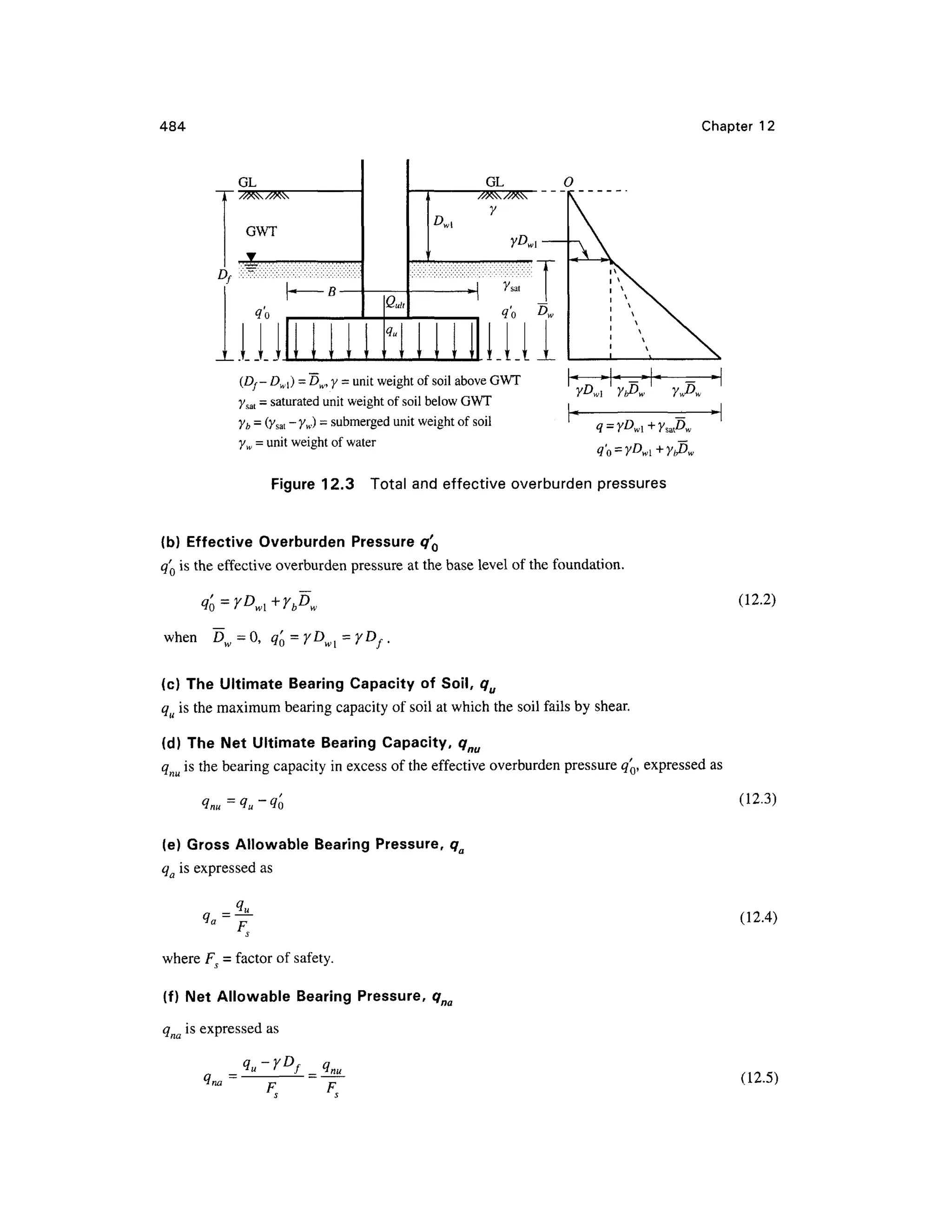
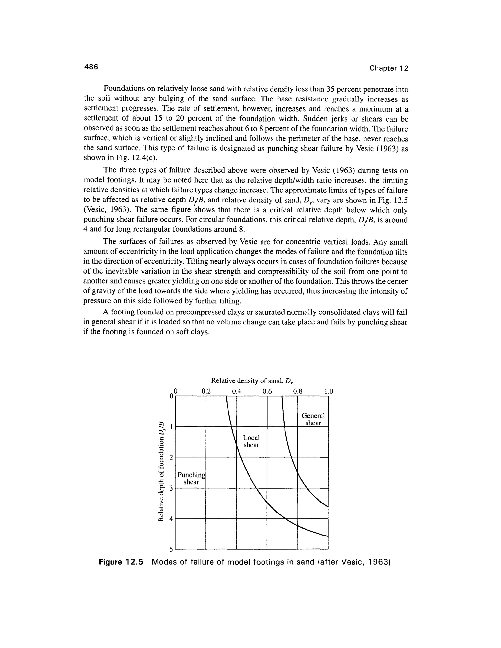
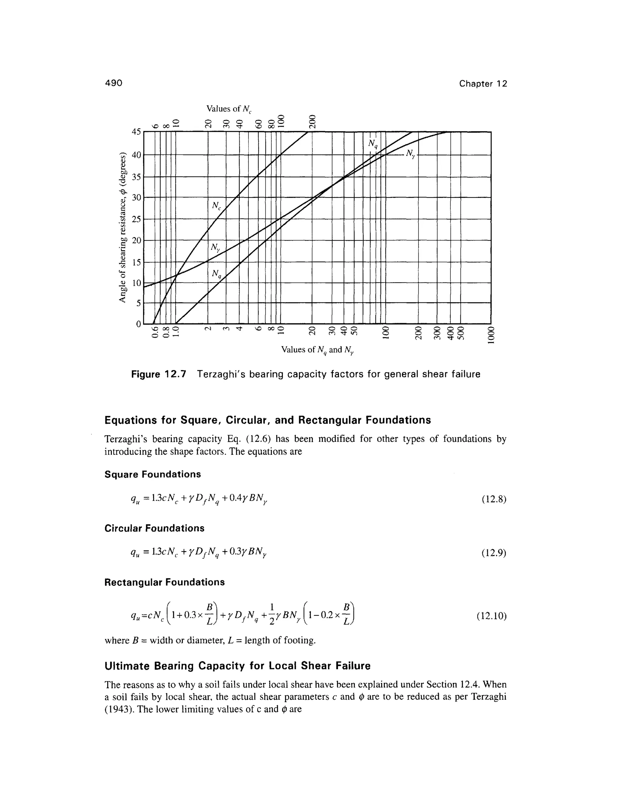
510. Shallow Foundatio n I : Ultimate Bearin g Capacity 49 1
c = 0.67 c
and ta n 0 = 0.67 tan</> o r 0 = tan'1
(0.67 tan<fi) (12.11 )
The equations for the lower bound values for the various types of footings are as given below.
Strip Foundatio n
qu = 0.61cNc+yDfNc/ + yBN y (12.12 )
Square Foundatio n
q + OAyBNy (12.13 )
Circular Foundatio n
qu = O.S61cNc+yDfN(] + 03yBNy (12.14 )
Rectangular Foundatio n
qu=Q.61c l + 0.3x
| N C +yD fNq +±yBN y l-02x | (12 .15)
where N , N an d N ar e the reduced bearing capacity factors for local shear failure. These factors
may be obtained either from Table 12.1 or Fig. 12.7 by making use of the friction angl e(f> .
Ultimate Bearin g Capacit y q u in Purely Cohesionles s an d Cohesiv e Soil s
Under Genera l Shea r Failur e
Equations for the various types of footings for (c - 0 ) soil under general shea r failure have been
given earlier. The same equations can be modified to give equations for cohesionless soil (for c = 0)
and cohesiv e soils (for</ > = 0) as follows.
It may be noted here that for c = 0, the value of Nc = 0, and for 0=0, the value of NC = 5.7 for
a strip footing and N = 1 .
a) Stri p Footin g
Forc = 0, q u= yDfNq+-yBNy (12.16 )
For 0 = 0, q u =5.7c + yDf
b) Squar e Footin g
For c = 0, q u = yDfNq+OAyBNr (12.17 )
For 0 =0, q u = 7.4c + yDf
c) Circula r Footin g
For c = 0, q u = yDfNq +Q3yBN y (12.18 )

511. 492 Chapter 1 2
For 0 = 0, q u = 7.4c + yDf
d) Rectangula r Footin g
For c = 0, q ii= yDfNq+-yBNY l-0.2 x — (12.19)
For 0-0 , o = 5.7 c l + 0.3x— + YD,
" L f
Similar types of equations as presented for general shea r failure can be developed fo r loca l
shear failure also.
Transition from Local to Genera l Shear Failure in Sand
As already explained, local shear failure normally occurs in loose an d general shea r failure occurs
in dense sand. There is a transition from loca l to general shear failure as the state of sand changes
140
120
100
1' 1 '
^
/ery Loose
- Loos e
Medium
Nm-
•^
>
y
/
"^
^v
/
/
Dense Ver y Dense
/
I/
V
^
N
/
//
/
^
/
/jAs
o
o
^
j
a
-
L
f
t
-
f
^
(
j
J
K
>
^
o
o
o
o
o
o
o
o
o
Standard
penetration
test
value,
N
cor
60
40
20
°28 3 0 3 2 3 4 3 6 3 8 4 0 4 2 4 4 4 6
Angle of internal friction, 0
Figure 12. 8 Terzaghi' s bearing capacit y factor s whic h take car e of mixe d stat e o f
local and general shear failures in sand (Pec k et al., 1974 )

512. Shallow Foundatio n I : Ultimate Bearin g Capacity 49 3
from loose to dense condition. There is no bearing capacity equation to account for this transition
from loose to dense state. Peck et al., (1974) have given curves for N an d N whic h automatically
incorporate allowance for the mixed state of local and general shear failures as shown in Fig. 12.8 .
The curves for N an d N ar e developed on the following assumptions.
1. Purel y local shear failure occurs when 0 < 28°.
2. Purel y general shear failure occurs when 0 > 38°.
3. Smoot h transition curves for values of 0 between 28° and 38° represent the mixed state of
local and general shear failures.
N an d Ny for values of 0 > 38° are as given in Table 12. 1. Values of N q an d N y fo r 0 < 28°
may be obtained from Table 12 . 1by making use of the relationship(f> - tan" 1
(2/3) tantf> .
In the case of purely cohesive soi l loca l shea r failur e may be assume d t o occur in sof t t o
medium stiff clay with an unconfined compressive strength qu < 100 kPa.
Figure 12. 8 als o give s the relationship between SP T valu e Ncor an d th e angl e o f internal
friction 0 by means of a curve. This curve is useful to obtain the value of 0 when the SPT value is
known.
Net Ultimat e Bearin g Capacit y an d Safety Facto r
The net ultimate bearing capacity qnu is defined as the pressure at the base level of the foundation in
excess of the effective overburden pressure q'Q = yD,as defined in Eq. (12.3). The net qnu for a strip
footing is
Similar expressions can be written for square, circular, and rectangular foundations and also
for local shear failure conditions.
Allowable Bearing Pressur
e
Per Eq. (12.4), the gross allowable bearing pressure is
1a=
^~ (12.21a )
In the same way the net allowable bearing pressure qna is
a Vu-yDf q nu
Vna - - p - - -p- (12.21b )
i S
where Fs = factor of safety which is normally assumed as equal to 3.
12.7 SKEMPTON' S BEARIN G CAPACIT Y FACTO R N C
For saturated cla y soils, Skempton (1951) proposed the following equation for a strip foundation
qu=cNc+yDf (12.22a )
or
4 m =4U- y°= cN
c (12.22b )

513. 494 Chapter 1 2
Figure 12. 9 Skempton' s bearin g capacit y facto r N c for cla y soil s
<lna=
-p- =
-J-(12.22C )
s s
The Nc values for strip and square (or circular) foundations as a function of the DJB ratio are
given in Fig. 12.9 . The equation for rectangular foundation may be written as follows
0.84 +0.16 x (12.22d)
where (NC)R = NC for rectangular foundation, (Nc)s = Nc for square foundation.
The lower and upper limiting values of Nc for strip and square foundations may be written as
follows:
Type of foundation
Strip
Square
Ratio D fIB
0
>4
0
>4
Value ofN c
5.14
7.5
6.2
9.0
12.8 EFFEC T O F WATER TABL E O N BEARIN G CAPACIT Y
The theoretica l equation s develope d fo r computin g th e ultimat e bearing capacit y q u o f soi l ar e
based on the assumption tha t the water table lies at a depth below th e base of the foundation equa l
to o r greate r tha n th e widt h B of the foundatio n or otherwise th e dept h o f the wate r tabl e fro m
ground surface is equal to or greater than (D,+ B). In case the water table lies at any intermediat e
depth less than the depth (D,+ B), the bearing capacity equations are affected due to the presence of
the water table .

514. Shallow Foundatio n I : Ultimate Bearin g Capacity 49 5
Two cases may be considered here .
Case 1. When the water table lies above the base of the foundation.
Case 2. When the water table lies within depth B below the base of the foundation.
We will consider th e two methods for determining the effect o f the water table on bearing
capacity as given below.
Method 1
For any position of the water table within the depth (ZX + B), we may write Eq. (12.6) as
qu=cNc+rDfNqRwl+±yBNyRw2 (12.23 )
where Rwl = reduction factor for water table above the base level of the foundation,
Rw2 = reduction factor for water table below the base level of the foundation,
7
= 7sat for all practical purposes in both the second and third terms of Eq. (12.23).
Case 1 : When th e wate r table lie s abov e th e bas e leve l o f the foundatio n or whe n Dwl/Df < 1
(Fig. 12.10a ) the equation for Rwl ma y be written as
For Dwl/Df= 0 , we have Rwl = 0.5, and for Dwl/Df= 1.0 , we have Rwl = 1.0.
Case 2: When the water table lies below the base level or when Dw2/B < 1 (12.1 Ob) the equation for
(12
'24b)
For Dw2/B = 0, we have Rw2 = 0.5, and for Dw2/B = 1.0, we have Rw2 = 1.0.
Figure 12.1 0 shows in a graphical form the relations Dwl/D,vs. Rwl an d Dw2/B v s Rw2.
Equations (12.23a) and (12.23b) are based on the assumption that the submerged unit weight
of soi l i s equa l t o hal f o f th e saturate d uni t weight and th e soi l abov e th e wate r tabl e remain s
saturated.
Method 2 : Equivalen t effective unit weigh t metho d
Eq. (12.6) for the strip footing may be expressed a s
Vu = cN
c+
YeiD
fN
q+re2BNY (12.25 )
where y el = weighted effective uni t weight of soil lying above the base level of the foundation
X?2 =
weighte d effectiv e uni t weigh t o f soi l lyin g withi n th e dept h B belo w th e bas e
level of the foundation
7 = moist or saturated unit weight of soil lying above WT (case 1 or case 2)

515. 496 Chapter 1 2
GWT
T i
D
Df
l.U
0.9
0.8
0.7
0.6
0.5(
/
/
/
/
/
) 0. 2 0. 4 0. 6 0. 8 1
(a) Water table above base level of foundation
Df
GWT
i.U
0.9
0.8
0.7
0.6
0.5(
^/
/
/
/
/
) 0. 2 0. 4 0. 6 0. 8 1
Submerged
(b) Water table below base level of foundation
Figure 12.1 0 Effec t o f W T o n bearin g capacit y
7sat = saturated unit weight of soil below the WT (case 1 or case 2)
Yb = submerged unit weight of soil = ysat - Y w
Case 1
An equation for yel ma y be written as
+ D^
' e ' b £)
f
(12.26a)
Case 2
Y e ~ y m

516. Shallow Foundatio n I : Ultimate Bearin g Capacity 497
Av2 /
' e2 > b f t 'm
v
-Yb) (12.26b)
Example 12. 1
A strip footing of width 3 m is founded at a depth of 2 m below the ground surface in a (c - 0 ) soil
having a cohesion c = 30 kN/m2
and angle of shearing resistance 0 = 35°. The water table is at a
depth of 5 m below ground level. The moist weight of soil above the water table is 17.25 kN/m3
.
Determine (a) the ultimate bearing capacity of the soil, (b) the net bearing capacity, and (c) the net
allowable bearing pressure and the load/m for a factor of safety of 3. Use the general shear failure
theory of Terzaghi.
Solution
2m
5m
0 1 CO
= 35
Y= 17.25 kN/m3
c = 30 kN/m2
Figure Ex. 12. 1
For 0 =35°
, N
c =57.8
, N=41.4, an
d N
y =42.
4
From Eq
. (12.6)
,
= 30 x57.8 +17.25 x 2 x41.4 + -x 17.25 x 3 x42.4 = 4259 kN/m2
^ =qu-yDf= 425 9 -17.25 x2 -4225 kN/m2
=
= 140
8 x3=422
5 kN/m

517. 498 Chapte r 12
Example 12.2
If the soil in Ex. 12. 1 fails b y local shear failure, determine the net safe bearing pressure. All the
other data given in Ex. 12. 1 remain the same.
Solution
For local shear failure :
0 = tan "'0.67 tan 35° =25°
c = 0.67'c = 0.67 x30 = 20 kN/m 2
From Table 12.1, fo r 0 = 25°, Nc = 25.1, N = 12.7, Ny = 9.7
Now from Eq . (12.12)
qu = 20 x25.1 +17.25 x2x 12.7 + -
x 17.25x3x9.7 = 1191 kN/m2
qm =1191-17.25x2 =1156.5 kN/m2
1156.50
*« = — = 385.5 kN/m2
Qa = 385.5x3 = 1156.5 kN/m
Example 12. 3
If the water table in Ex. 12. 1 rises to the ground level, determine the net safe bearing pressure of the
footing. All the other data given in Ex. 12. 1 remain the same. Assume the saturated unit weight of
the soil ysat= 18.5 kN/m3
.
Solution
When the WT is at ground level we have to use the submerged unit weight of the soil .
Therefore y , = y - y = 18.5 -9.81 =8.69 kN/m3
' u ' Sa l * W
The net ultimate bearing capacity is
qnu = 30 x 57.8 + 8.69 x 2(41.4 - 1 ) + -x 48.69 x 3 x42.4 «2992 kN/m2
2992
qm=—^- = 997.33 kN/m2
Q = 997.33x 3 = 2992 kN/m
Example 12. 4
If th e wate r tabl e i n Ex . 12. 1 occupies an y o f th e position s (a ) 1.2 5 m belo w groun d leve l o r
(b) 1.2 5 m below th e base level of the foundation, what will be the net safe bearing pressure ?
Assume ysat = 18.5 kN/m3
, /(above WT) = 17.5 kN/m3
. All the other data remain the same as
given in Ex. 12.1 .

518. Shallow Foundation I: Ultimate Bearing Capacity 49 9
Solution
Method 1 —By making use of reduction factors Rwl an d Rw2 and using Eqs. (12.20 ) an d (12.23) ,
we may write
1
nu c f q w 2 '
Given: N = 41.4, Ny = 42.4 and Nc = 57.8
Case I—When the WT is 1.25 m below the GL
From Eq. (12.24), we get Rwl = 0.813 for Dw/Df= 0.625 , Rw2 = 0.5 for Dw2/B = 0.
By substituting the known values in the equation for qnu, we have
qm = 30x57.8 + 18.5x2x40.4x0.813 + -xl8.5x3x42.4x0.5 = 3538 kN/m2
= 1179 kN/m2
3
Case 2—When the WT is 1.25 m below the base of the foundation
R , = 1.0 for D ,/Z X =1, R , =0.71 fo r D JB = 0.42.
wl w l / ' w 2 w2
Now the net bearing capacity is
qm = 30x57.8 + 18.5x2x40.4xl + -xl8.5x3x42.4x0.71 =4064 kN/m2
= 1355
Method 2 —Usin
g the equivalent effective uni t weight method.
Submerged unit weight yb = 18.5 - 9.8 1 = 8.69 kN/m3
.
Per Eq. (12.25 )
The net ultimate bearing capacit y i s
q = c N + y , D f ( N -l) + -y7 BNV
"nu c ' el f ^ q ' n ' e2 y
Case I—When D wl = 7.25 m (Fig. Ex. 12.4)
From Eq. (12.26a)
f
where y - y . =18.5 kN/m3
' 77 1 * Sal
125
yel = 8.69 +— (18.5-8.69) = 14.82 kN/m3
re2=rb =8.69 kN/m3
o= 30 x57.8 +14.82 x 2 x40.4 + -x 8.69 x 3 x42.4 = 3484 kN/m2

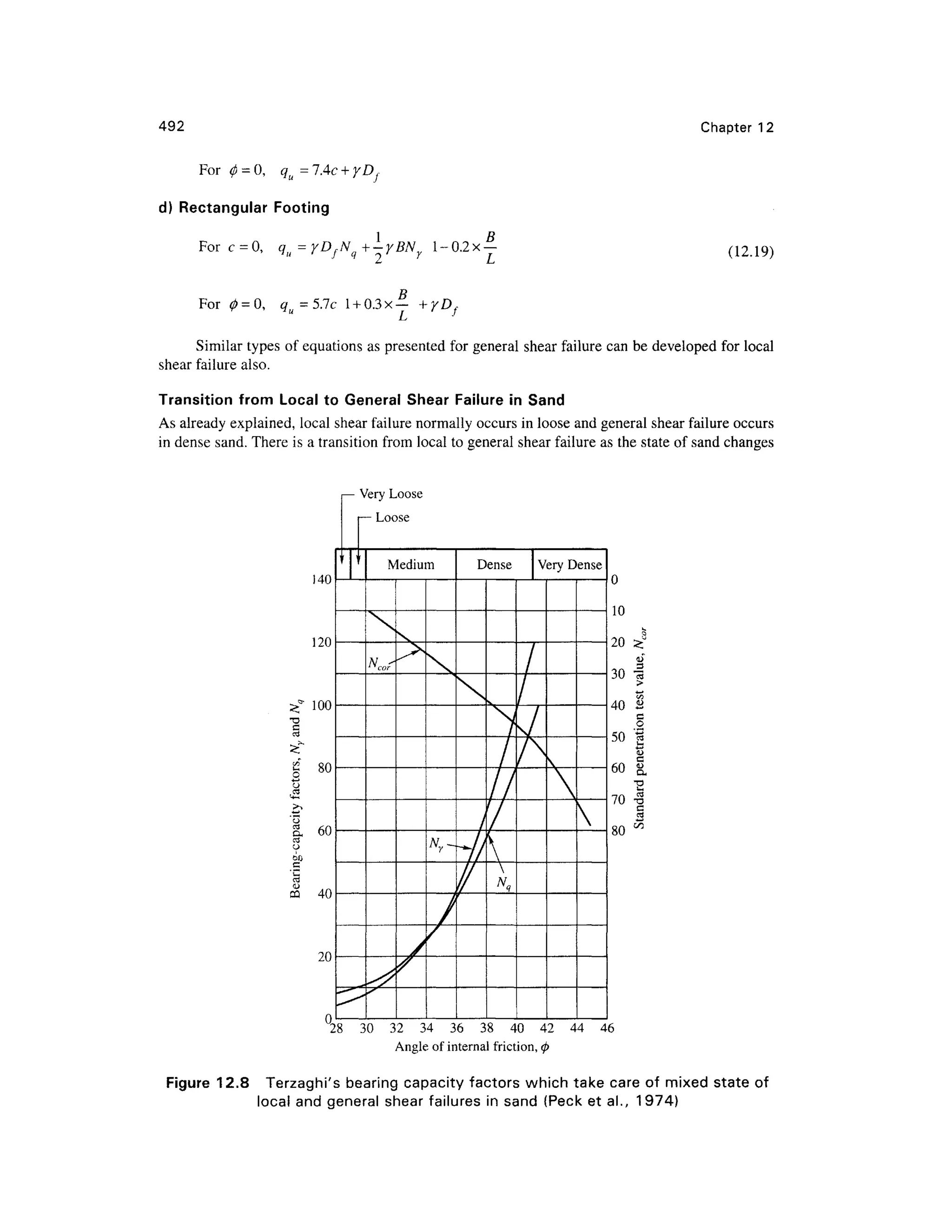
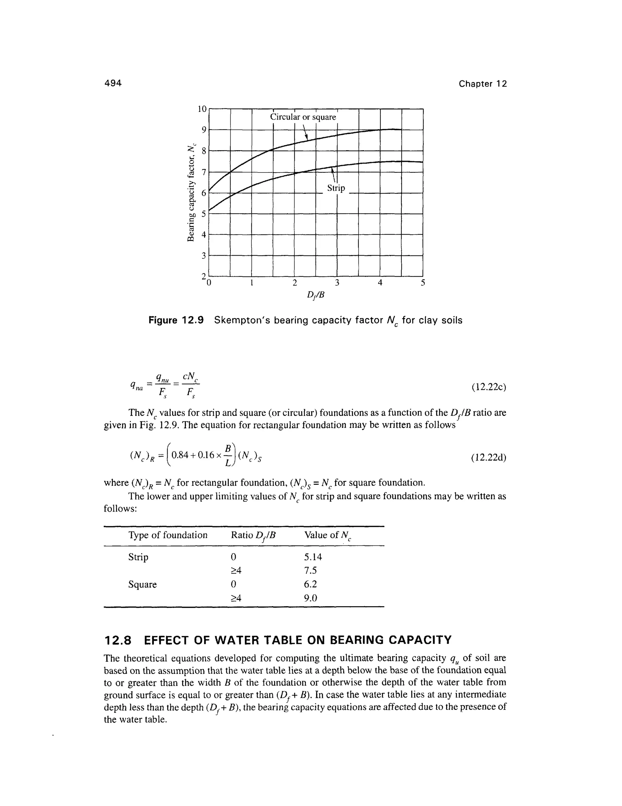
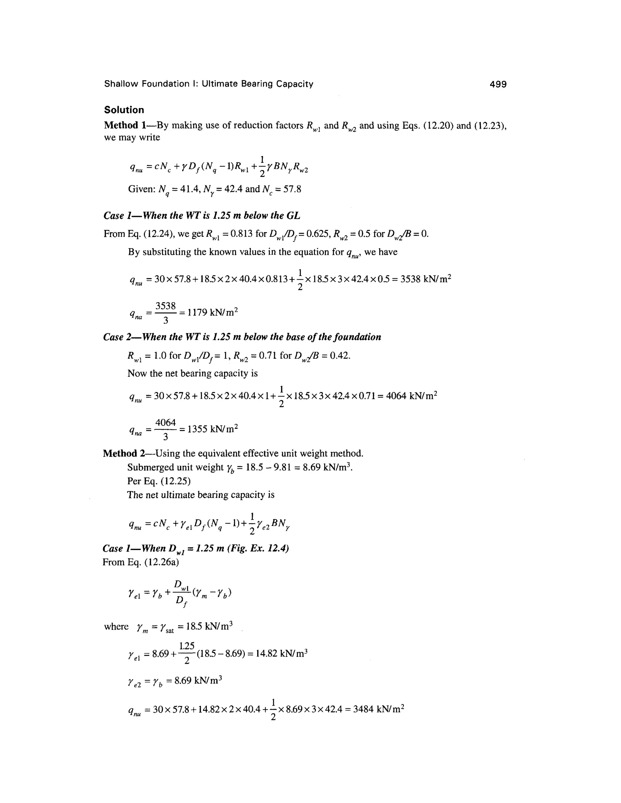
519. 500 Chapter 1 2
GL
"1
2
1
m
J
'
s S/K
L
-* —- 3 m - _HC,., =1.25m
1 . T f
t
Dw2= 1.25m
T 1
K
Case 1
Case 2
Figure Ex. 12. 4 Effec t of W T o n bearing capacit y
3484
Case 2—When Dw2 = 1.25 m (Fig. Ex. 12.4)
FromEq. (12.26b)
y=y = 18.5kN/m 3
* el ' m
1.25
y , =8.69 + —-(18.5- 8.69) = 12.78 kN/m3
€ L 4.
= 30x57.8 +18.5x2x40.4+ -
x 12.78x3x42.4 = 4042 kN/m2
4042
= 1347 kN/m2
Example 12. 5
A squar e footin g fail s b y genera l shea r i n a cohesionles s soi l unde r a n ultimat e loa d o f
Quh - 1687. 5 kips. The footing is placed at a depth of 6.5 ft below ground level. Given 0 =35°, and
7=110 Ib/ft3
, determin e the size of the footing if the water table is at a great depth (Fig. Ex. 12.5).
Solution
For a square footing [Eq. (12.17)] for c = 0, we have
For 0= 35° , Nq = 41.4, and Wy= 42.4 from Table 12.1 .

520. Shallow Foundatio n I: Ultimate Bearin g Capacit y 501
6.5ft
Qul!= 1687. Skip s
0 = 35°, c = 0
y= 11 0 lb/ft3
BxB - |
Figure Ex. 12. 5
_ Q u _ 1687.5xlO 3
qu
~~B^~ 5 2
By substituting known values, we have
1 87
'5xl
— = 110 x 6.5 x 41.4 + 0.4 x110 x 42.45
/?
= (29.601 +1.8665)103
Simplifying and transposing, we have
53
+ 15.86352
-904.34 = 0
Solving this equation yields, 5 = 6.4 ft.
Example 12. 6
A rectangular footing of size 1 0 x 20 ft is founded at a depth of 6 ft below the ground surface in a
homogeneous cohesionles s soi l having an angle of shearing resistance 0 =35°. The water table is at
a great depth. The unit weight of soil 7= 114 lb/ft3
. Determine: (1) the net ultimate bearing capacity,
y= 114 lb/ft3
- 10x2 0 ft
Figure Ex. 12. 6

521. 502 Chapte r 1 2
(2) the net allowable bearing pressure for FV = 3, and (3) the allowable load Qa the footing can carry.
Use Terzaghi's theory. (Refer to Fig. Ex. 12.6)
Solution
Using Eq. (12.19) and Eq. (12.20) fo r c - 0 , the net ultimate bearing capacity for a rectangular
footing i s expressed a s
From Table 12.1 , N = 41.4, Ny = 42.4 for 0 = 35°
By substituting the known values,
q= 114x6(41.4-l ) + -xll4xlOx42.4 l-0.2x — = 49,38 5
2 2 0
49 385
qna = —
= 16,462 lb/ft 2
Qa = (B x L)qna = 10 x 20 x 16,462- 3,292 xlO3
I b = 3292 kip s
Example 12. 7
A rectangular footing of siz e 1 0 x 2 0 ft is founded at a depth of 6 ft below th e groun d level in a
cohesive soil (0 = 0) which fails b y general shear. Given: ysal =114 lb/ft3
, c = 945 lb/ft2
. The water
table i s close t o the ground surface. Determine q , q an d qna by (a) Terzaghi's method , and (b)
Skempton's method . Use Fv = 3.
Solution
(a) Terzaghi's metho d
Use Eq. (12.19)
For 0= 0° , Nc = 5.7, N = I
qu=cNc l+0.3x | +y hDf
Substituting the known values ,
qu = 945x5. 7 l + 0.3x— +(114-62.4)x 6 ='6,504 lb/ft 2
qm = (qu ~ yb Df) = 6504 - (11 4 - 62.4 ) x 6 =6195 lb/ft 2
lb/ft2
™ F y 3
(b) Skempton's method
From Eqs . (12.22a) and (12.22d) we may write

522. Shallow Foundatio n I : Ultimate Bearin g Capacit y 50 3
where Ncr = bearing capacity factor for rectangular foundation.
Ncr = 0.8 4 + 0.16 x — xN
where Ncs = bearing capacit y factor for a square foundation.
From Fig. 12.9, Ncs = 7.2 for Df/B = 0.60.
Therefore N c = 0.8 4 + 0.16 x— x 7.2 =6.62
20
Now q u = 945 x6.62 + 114 x6 = 6940 lb/ft 2
qnu =(qu-YD") = 6940 -114x6 = 6,256 lb/ft 2
= 2
Note: Terzaghi's an d Skempton's values are in close agreement for cohesive soils .
Example 12.
8
If the soil in Ex. 12. 6 is cohesionless ( c = 0), and fails in local shear , determin e (i ) the ultimate
bearing capacity, (ii) the net bearing capacity, and (iii) the net allowable bearing pressure. All the
other data remain the same.
Solution
From Eq. (12.15) and Eq. (12.20), the net bearing capacity for local shear failure for c - 0 is
q^bu-YDf^YDfWq-D + ^YBNy l~0.2x |
whereJZ > = tan"1
0.67 tan 35° -25°, J V = 12.7, an d N = 9.7 fo r 0 = 25° fro m Table 12.1.
By substituting known values, we have
tfn=114x6(12.7-l) + -xll4xlOx9.7 l-0.2 x — = 12,979 lb/ft 2
tnu 2 2 0
12979
V = - = 4326 lb/ft2
12.9 TH E GENERAL BEARIN G CAPACIT Y EQUATIO N
The bearing capacity Eq. (12.6) developed b y Terzaghi i s for a strip footing under general shea r
failure. Eq . (12.6) has been modifie d for other types of foundations such as square, circula r and
rectangular by introducing shape factors. Meyerhof (1963 ) presented a general bearing capacit y
equation whic h takes int o accoun t th e shap e an d th e inclinatio n of load . Th e genera l for m of
equation suggested by Meyerhof for bearing capacity is

523. 504 Chapte r 1 2
where c - uni t cohesion
g'o = effectiv e overburde n pressure at the base level of the foundation = Y®f
y= effectiv e uni t weight above the base level of foundation
7 = effectiv e uni t weight of soil below the foundation base
D, = dept h of foundation
sc, s , s= shap e factors
dc, d , d= dept h factor
/c, / , i= loa d inclination factors
B = widt h of foundatio n
Nc, N , N= bearin g capacity factors
Hansen (1970 ) extende d the work of Meyerhof b y including in Eq. (12.27 ) two additional
factors to take care of base tilt and foundations on slopes. Vesic (1973, 1974) used the same form of
equation suggested by Hansen. All three investigators use the equations proposed by Prandtl (1921)
for computing the values of Nc an d N wherei n the foundation base is assumed as smooth with the
angle a = 45° + 0/2 (Fig. 12.6). However, the equations used by them for computing the values of
N ar e different. Th e equations for Nc, N an d N ar e
Table 12. 2 Th e values of A/ , /V . and Meyerhof (M) , Hanse n (H ) and Vesic (V ) N
c q 7
Factors
0
0
5
10
15
20
25
26
28
30
32
34
36
38
40
45
50
N
c
5.14
6.49
8.34
10.97
14.83
20.71
22.25
25.79
30.13
35.47
42.14
50.55
61.31
72.25
133.73
266.50
Nq
1.0
1.6
2.5
3.9
6.4
10.7
11.8
14.7
18.4
23.2
29.4
37.7
48.9
64.1
134.7
318.50
/VX(H)
0.0
0.1
0.4
1.2
2.9
6.8
7.9
10.9
15.1
20.8
28.7
40.0
56.1
79.4
200.5
567.4
/Vr(M)
0.0
0.1
0.4
1.1
2.9
6.8
8.0
11.2
15.7
22.0
31.1
44.4
64.0
93.6
262.3
871.7
A/y(V)
0.0
0.4
1.2
2.6
5.4
10.9
12.5
16.7
22.4
30.2
41.0
56.2
77.9
109.4
271.3
762.84
Note: NC and N ar e the same for al l the thre e methods. Subscripts identify th e autho r for N .

524. Shallow Foundation I: Ultimate Bearing Capacit y 505
Table 12. 3 Shape , depth and load inclination factors o f Meyerhof , Hansen and
Vesic
Factors Meyerhof Hansen Vesic
1 + 0.2N,—
<* L
1 +0.1A^ — fo r <f»Q°
L
s = s fo r 0>IQ°
s — s= 1 fo r 0 =0
i— D f
/ —D
f
1 +O.UA^ —*- fo r
dy = dq fo r</> > 10°
d=d = l fo r ^ =
1 a
*
1 fo r any
90
iq = ic fo r any 0
1- — fo r
ir=0 fo r ^ =
5
1 +— tan^
1-0.4-
L
1 +0.4
B
1 fo r al l<f>
Note; Vesic's s and Jfactors
= Hansen's s and d factors
for 0>0
g
N - 1
iT
±
0.5 1--^- 2
for 0 =0
The shape and depth factors
of Vesic are the same as those
of Hansen.
Same as Hansen for > 0
1--
Ny = (Nq - 1) tan(1.40) (Meyerhof )
Ny = l.5(Nq - 1) tan 0(Hansen )
Ny=2(Nq+l)ten</> (Vesic )
Table 12.2 gives th e values of the bearing capacit y factors. Equation s fo r shape , dept h an d
inclination factors are given in Table 12.3 . The tilt of the base and the foundations on slopes are not
considered here .
In Table 12. 3 The following terms are defined with regard t o the inclination factors
Qh = horizonta l componen t o f the inclined load
Qu = vertica l component of the inclined load

525. 506 Chapte r 1 2
ca = uni t adhesion on the base of the footing
A, = effectiv e contac t area of the footing
_
m
~ m
~
_
m
~ m
~
_
B ~ i +B/Lwit h Qh parallel to B
2 + B/L
l + B/Lwit h Qh parallel to L
The general bearin g capacity Eq. (12.27) has not taken into account the effect o f the water
table positio n o n th e bearin g capacity . Hence , Eq . (12.27 ) has t o be modifie d accordin g t o the
position of water level in the same way as explained in Section 12.7 .
Validity o f th e Bearin g Capacit y Equation s
There is currently no method of obtaining the ultimate bearing capacity of a foundation other than
as an estimate (Bowles, 1996). There has been little experimental verification of any of the methods
except by using model footings. Up to a depth of Df~ B the Meyerhof q u is not greatly differen t
from th e Terzaghi valu e (Bowles, 1996) . The Terzaghi equations, being th e firs t proposed , hav e
been quite popular with designers. Both the Meyerhof and Hansen methods are widely used. Th e
Vesic method has not been much used. It is a good practice to use at least two methods and compare
the computed values of qu. If the two values do not compare well , use a third method.
Example 12. 9
Refer to Example 12.1 . Compute using the Meyerhof equation (a) the ultimate bearing capacity of
the soil, (b) the net bearing capacity, and (c) the net allowable bearing pressure. All the other data
remain the same.
Solution
Use Eq. (12.27). For i = 1 the equation for net bearing capacity is
- }s qdq
From Table 12. 3
D
sc - 1 + 0.2A — = 1 for strip footing
n
5 = 1 +Q.N — = 1 fo r strip footing
JLv
d = l + 0.2/v7 — -= l + 0.2tan 45°+ — - = 1.25 7
B
^ cr
=1 +0.
1 tan 45°+ — - = 1.12 9
2 3
dy=dq=U29

526. Shallow Foundatio n I : Ultimate Bearin g Capacity 50 7
From Ex. 12.1, c= 30 kN/m2
, y =17.25 kN/m3
, Df= 2 m , B = 3 m.
From Table 12.2 for 0= 35 ° we have A/c = 46.35,AT = 33.55, Ny= 37.75 . Now substituting the
known values, we have
qm = 30 x46.35 x 1 x 1.257 +17.25 x 2 x(33.55 -1) x 1 x1.129
+ - x 17.25 x 3 x37.75 x 1 x1.129
2
= 1,748 + 1,268 +1,103 =4,1 19 kN/m2
1na=—^ = 1373 kN/m2
There is very close agreement between Terzaghi's and Meyerhof 's methods.
Example 12.10
Refer to Example 12.6. Compute by Meyerhof 's method the net ultimate bearing capacity and the
net allowable bearing pressure for Fs = 3. All the other data remain the same.
Solution
From Ex. 12.6 we have B = 10 ft, L = 20 ft, Df= 6 ft, and y= 1 14 lb/ft3
. From Eq. (12.27) for c = 0
and / = 1 , we have
From Table 12.3
D O C 1 f
sa = 1 +0.1AL - = 1 +0.1 tan2
45°+ — — = 1.18 5
q
* L 2 2 0
d = l + O.L/A/7 -^ = l + 0.1tan 45°+ — — = 1.11 5
v V 0 B 2 1 0
^=^=1.115
From Table 12. 2 for</ > = 35°, we have N = 33.55, N = 37.75. By substitutin g the known
values, we have
qm =114x6(33.55-l)xl.l85xl.ll5 + -xll4xlOx37.75xl.l85xl.ll5
= 29,417 + 28,431 =57,848 lb/ft 2
lb/ft2
By Terzaghi's method qm = 16,462 lb/ft 2
.
Meyerhof's method gives a higher value for qna by about 17%.

527. 508 Chapte r 1 2
Example 12.1 1
Refer to Ex. 12.1 . Compute by Hansen's metho d (a) net ultimate bearing capacity, an d (b) the net
safe bearing pressure. All the other data remain the same.
Given for a strip footing
B = 3 m, Df = 2m, c = 30 kN/m2
and y =17.25 kN/m3
, Fs - 3 .
From Eq . (12.27 ) for / = 1 , we have
From Table 12. 2 for Hansen's method, we have for 0 = 35c
Nc = 46.35, N q = 33.55, an d Ny= 34.35 .
From Tabl e 12. 3 we have
o
s = 1 H — — = 1 fo r a strip footing
N L
D
s = 1H— tan(/) = 1 fo r a strip footing
D
s - 1 - 0.4— = 1 fo r astrip footing
D
f 2
d = 1 + 0.4-^- = l + 0.4x- = 1.267
0
B 3
Df
-^
= l + 2tan35°(l-sin35°)2
x-=l + 2x0.7(1- 0.574)2
x-=1.17
Substituting the known values, we have
qnu = 30 x46.35 x 1 x 1.267 +1 7.25 x 2 x(33.55 -1) x 1 x1.1 7
+ -Xl7.25x3x34.35xlxl
2
= 1,762 +1,3 14 + 889 = 3,965 kN/m 2
= U22 kN/m2
The values of qna by Terzaghi, Meyerhof and Hansen methods are
Example Autho r q na kN/m2
12J Terzagh i 1,40 8
12.9 Meyerho f 1,37 3
12.11 Hanse n 1,32 2

528. Shallow Foundatio n I : Ultimate Bearin g Capacity 50 9
Terzaghi's method is higher than Meyerhof 's by 2.5% and Meyerhof 's higher than Hansen's by
3.9%. The difference between the methods is not significant. Any of the three methods can be used.
Example 12.1 2
Refer to Example 12.6 . Compute the net safe bearing pressure by Hansen's method. All the other
data remain the same.
Solution
Given: Size 1 0 x 20 ft, Df= 6 ft, c = 0, 0 = 35°, y= 1 14 lb/ft3
, Fs = 3.
For 0 = 35° we have from Table 12.2 , Nq = 33.55 and Ny = 34.35
From Table 12. 3 we have
/? 1 0
5 = 1 +— tan0=
l + — xtan35° = 1.35
q
L 2 0
D i n
sv = 1-0.4 — =l-0.4x — = 0.80
7
L 2 0
dq = 1+ 2tan 35° (1 - sin 35° )2
x — = 1.153
Substituting the known values, we have
-l)Sqdg +
= 1 14 x6(33.55 -1) x1.35 x1.153 +-x 114 x10 x 34.35 x 0.8 x 1
2
= 34,655 +15,664 = 50,319 lb/ft2
50,319
The values of qna by other methods are
Example Autho r q kN/m 2
12.6 Terzagh i 16,46 2
12.10 Meyerho f 19,28 3
12.12 Hanse n 16,77 3
It can be seen from the above, the values of Terzaghi and Hansen are very close to each other,
whereas the Meyerhof value is higher than that of Terzaghi by 1 7 percent.
12.10 EFFEC T O F SOIL COMPRESSIBILIT Y O N BEARIN G
CAPACITY O F SOI L
Terzaghi (1943) develope d Eq . (12.6) based on the assumption that the soil is incompressible. I n
order to take into account the compressibility of soil, he proposed reduced strength characteristics
c and 0 defined by Eq. (12.11). As per Vesic (1973) a flat reduction of 0 in the case of local and

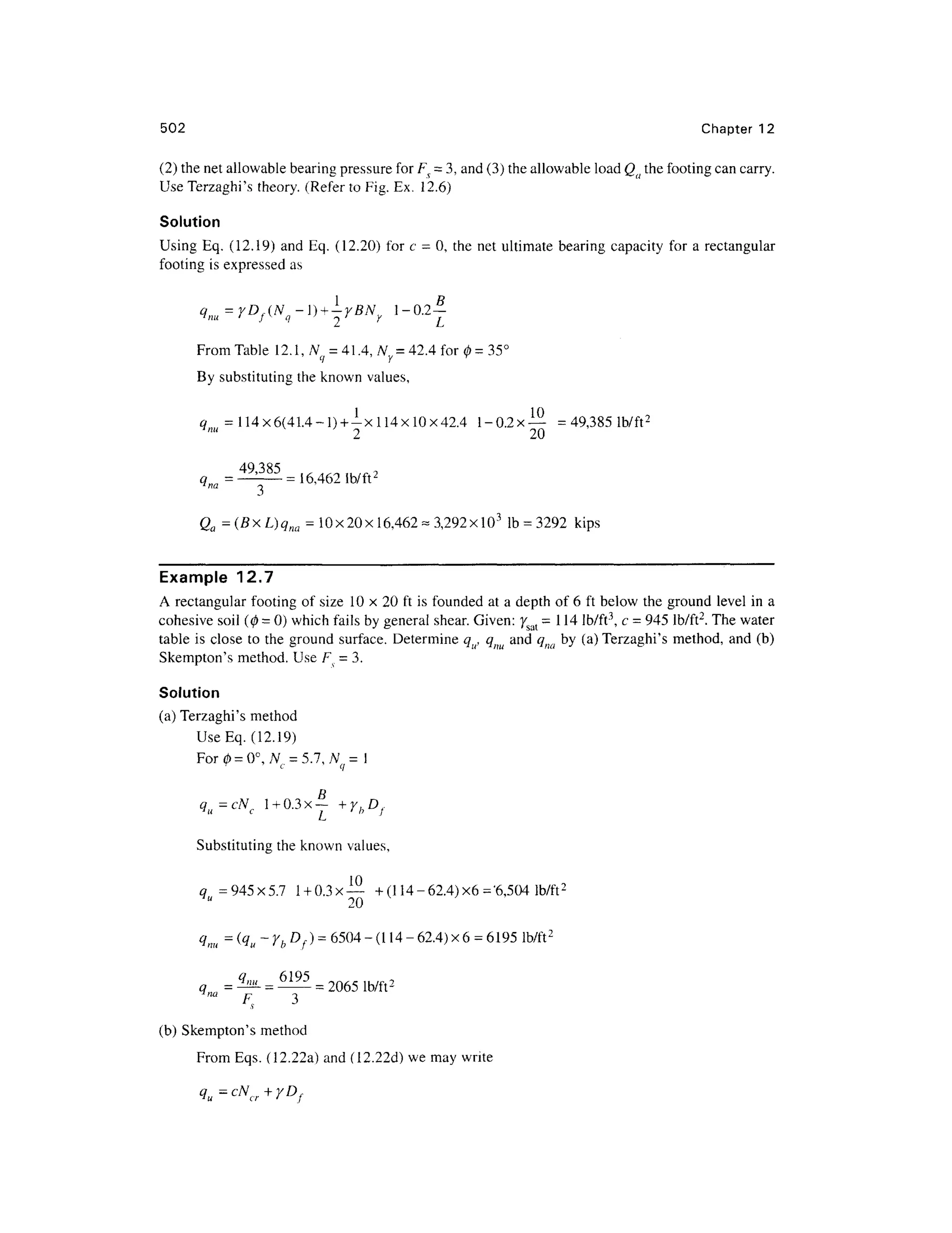
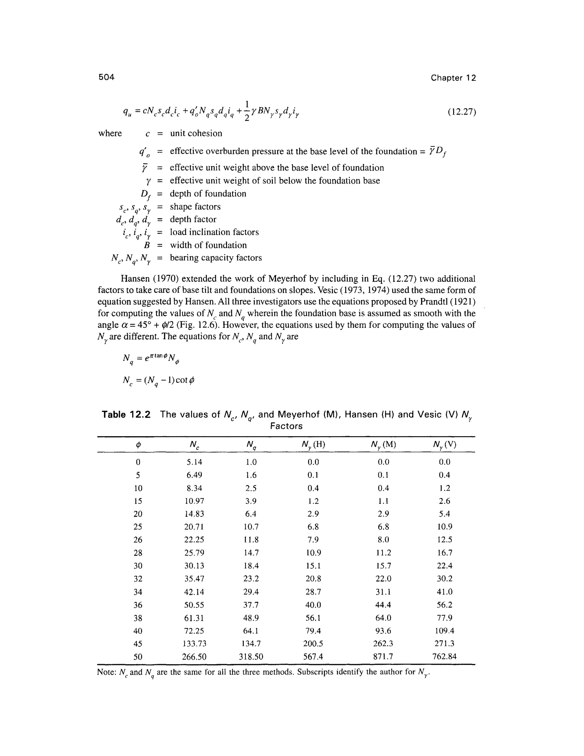
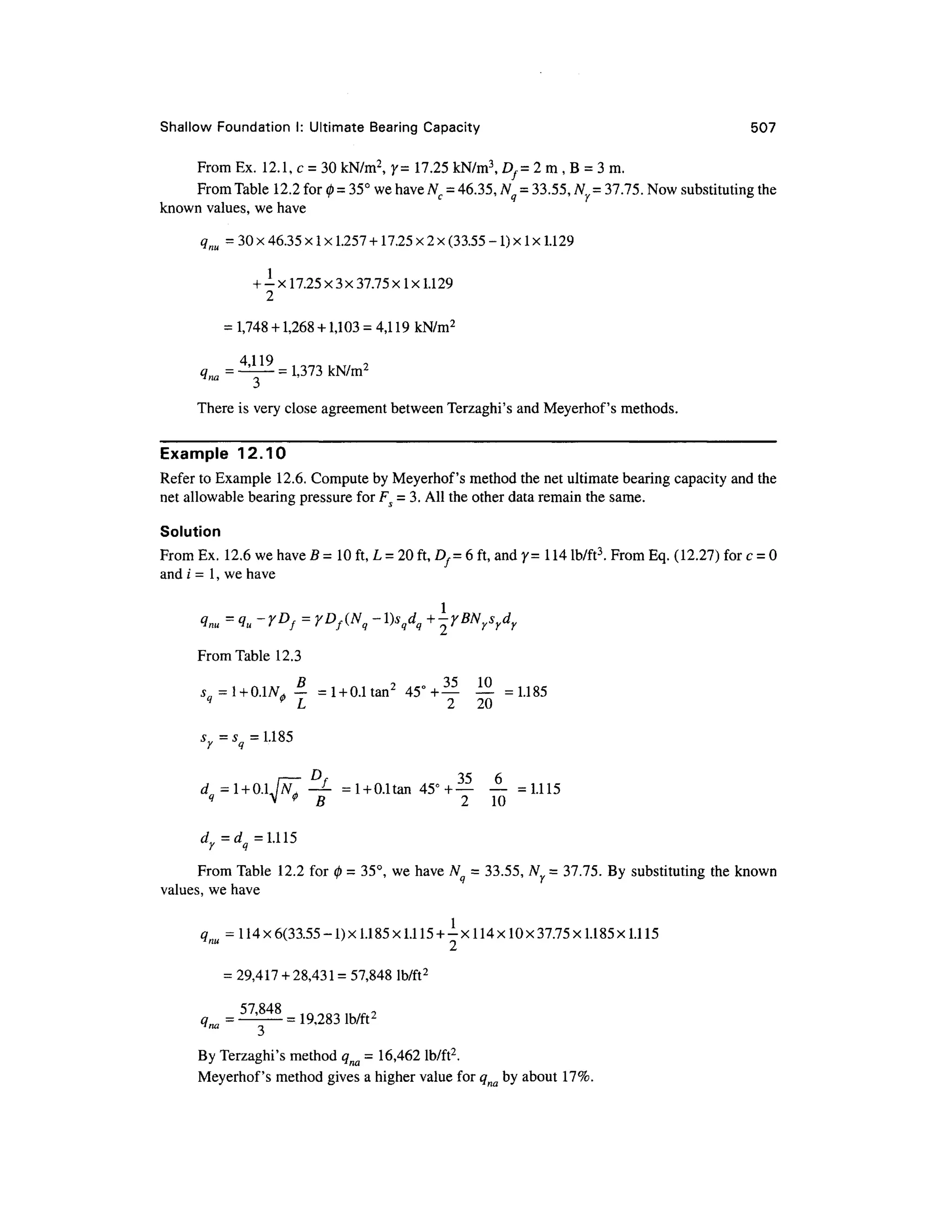
529. 510 Chapter 1 2
punching shear failure s i s too conservative and ignores th e existence o f scale effects. It has bee n
conclusively established tha t the ultimate bearing capacity qu of soil does not increase in proportion
to the increase i n the size of the footing as shown in Fig. 12.1 1 or otherwise the bearing capacit y
factorA f decrease s with the increase in the size of the footing as shown in Fig. 12.12 .
In order to take into account the influence of soil compressibility and the related scale effects ,
Vesic (1973 ) propose d a modificatio n o f Eq . (12.27 ) b y introducin g compressibilit y factor s a s
follows.
qu = cN
cdcscCc+q'oNqdqsqCq + (12.28)
where, C c, C an d C ar e the soil compressibility factors. The other symbol s remain th e same as
before.
For th e evaluatio n o f the relativ e compressibilit y o f a soi l mas s unde r loade d conditions,
Vesic introduced a term called rigidity index Ir, which is defined as
/ =
c + qtar0 (12.29)
where, G = shea r modulu s of soil = ^( +u]
Es = modulu s of elasticity
q = effectiv e overburden pressure at a depth equal to (ZX + 5/2 )
600
400
200
100
80
60
3 4 0
20
10
8
6
4
2
1
I I T
Circular footing s
Chattahoochee san d (vibrated)
Dry unit weight, 96.4 lb/ft 3
Relative density, Dr = 0.79
Standard triaxial, 0= 39°
Deep penetration resistanc e
(Measured) (Postulated ) V ;
Test plate size s
Dutch cone size - * *
II I I I I I
Usual footing size s
I I I I I I
0.2 0.40.60.81. 0 2 4 6 8 10
Footing size, ft
20 40 608010 0 20 0
Figure 12.1 1 Variatio n o f ultimat e resistanc e o f footings with size
(after Vesic , 1969 )

530. Shallow Foundatio n I: Ultimate Bearin g Capacit y 511
800
600
400
200
Gent, yk = 1.674 ton/m3
Vesic,
yk= 1.538 ton/m3
Meyerhof,
y k= 1.70ton/m 3
vv s Golder ,
Circular plates
Square plates
Rectangular plates
-> Gent , yk = 1.619 ton/m3
Gent,yfc= 1.50 9 ton/m3
® Meyerhof , yk = 1.62 ton/m3
Meyerhof, yk = 1.485 ton/m3
0
Vesic , yk = 1.440 ton/m3
yk = 1.76 ton/m
C* /—vai n
•Vandeperre, yk = • 1.647 ton/m
Meischeider, yk =1/788 ton/m3
'
A
Muhs
0.01 0.02 0.03 0.0 4
yB, kg/cm2
0.05 0.06 0.07 •M,
100
Figure 12.1 2 Effec t of size on bearing capacity o f surface footings in sand (After
De Beer, 1965)
^ = Poisson' s ratio
c, 0 = shea r strength parameters
Eq. (12.29) was developed o n the basis of the theory of expansion of cavities in an infinit e
solid wit h th e assume d idea l elasti c propertie s behavio r o f soil . I n orde r t o tak e car e o f th e
volumetric strai n A i n th e plasti c zone , Vesi c (1965 ) suggeste d tha t th e valu e o f I r, give n by
Eq. (12.29), be reduced by the following equation.
I=FrI (12.30 )
where F. =reduction factor =
/ A
It is known that Ir varies with the stress level and the character of loading. A high value of Irr,
for example over 250, implies a relatively incompressible soil mass, whereas a low value of say 10
implies a relatively compressible soi l mass.
Based on the theory of expansion of cavities, Vesic developed the following equation for the
compressibility factors.
B 3.0 7 sinolog 21
C = ex p -4. 4 +0.6— tan0 + ^ 5 r
q
L l +sin<z>
For 0 > 0, one can determine fro m the theorem of correspondenc e
C = C -
c
For 0 = 0, we have
C = 0.3 2 +0.12— + 0.6 log/
L
(12.31)
(12.32)
(12.33)

531. 512 Chapter 1 2
/ =
G
r
c+qtan(j>
0
10 20 20
30 4 0 5 0 0 1 0
Angle o f shearin g resistance,(J >
Figure 12.1 3 Theoretica l compressibilit y factor s (afte r Vesic , 1970 )
For all practical purposes , Vesic suggest s
C = C.. (12.34)
Equations (12.30 ) throug h Eq. (12.34) ar e valid as long as the values of the compressibilit y
factors ar e less tha n unity. Fig. 12.1 3 shows graphically the relationship betwee n C ( = C ) and 0
for two extreme cases ofL/B > 5 (strip footing) and B/L = 1 (square) for different values of Ir (Vesic
1970). Vesi c gives another expression calle d the critical rigidity index (I r)cr expresse d a s
Table 12. 4 Value s o f critica l rigidit y inde x
Angle of shearin g resistance Critica l rigidity index fo r
Strip foundation Squar e foundation
(t) B/L = 0 B/L = 1
0
5
10
15
20
25
30
35
40
45
50
13
18
25
37
55
89
152
283
592
1442
4330
8
11
15
20
30
44
70
120
225
486
1258

532. Shallow Foundatio n I: Ultimate Bearin g Capacity 51 3
(Ur=f*p 3.3-0.45- ? cot(45-0/2 ) (1 2 35)
The magnitud e of (I) cr fo r any angle of 0 and any foundation shape reduces th e bearing
capacity because of compressibility effects. Numerical values of (l)cr fo r two extreme cases ofB/L
= 0 and BIL = 1 are given in Table 12. 4 for various values of 0.
Application of /, (or /„) an d (/r)crit
1 .I f lr (or Irr) > (/r)crit, assume the soil is incompressible and C, = C = C = I i n Eq. (12.28).
2. I f Ir (o r Irr) < (/r)crit, assume the soil i s compressible. I n such a case the compressibilit y
factors Cc, C and C are to be determined and used in Eq. (12.28).
The concept and analysis developed above by Vesic (1973) are based on a limited number of
small scale model tests and need verification in field conditions.
Example 12.1
3
A square footing of size 1 2 x 1 2 ft is placed a t a depth of 6 ft in a deep stratum of medium dense
sand. The following soil parameters ar e available:
Y = 100 lb/ft3
, c = 0, 0 = 35°, Es = 100 t/ft2
, Poissons' rati o n = 0.25
.
Estimate the ultimate bearing capacity by taking into account the compressibility o f the soil
(Fig. Ex. 12.13) .
Solution
E
Rigidity / = -
s
- -
fo r c= 0from Eq. (12.29)
r
q = y(Df + 5/2) = 100 6 +—= 1,200 lb/ft2
= 0.6 ton/ft 2
Neglecting the volume change in the plastic zone
/,= _
!° ° _
= 95
r
2( 1 +0.25)0.6 tan 35°
From Table 12.4 , (7r)crit = 120 for 0 = 35°
Since /. < (/r)crit, the soil is compressible.
From Fig. 12.13, Cq (= Cy) = 0.90 (approx) for square footing for 0 = 35° and /. =95.
From Table 12.2, Nq = 33.55 and Wy = 48.6 (Vesic's value)
Eq. (12.28) may now be written as
I
2
From Table 12.3
u = q'0NqdqsqCq +-yBN ydrsrCr
D
s = 1 + —tan^=
l + tan35° =1.7 fo r B = L
j = 1-0.4 = 0.6 forf i = L

533. 514 Chapter 1 2
dn =
q
2tan35°(l-sin35°)2
x— = 1.127
12
<7o = 100x6 = 600 lb/ft 2
Substituting
qu = 600 x33.55 x1.1 27 x 1.7 x 0.90 + -x 100 x1 2 x48.6 x 1.0 x 0.6 x0.90
= 34,710 + 15,746 = 50,456 lb/ft 2
If the compressibility factors are not taken into account (That is, C = C = 1) the ultimate
bearing capacity qu is
qu = 38,567 + 17,496 = 56,063 lb/ft 2
,
6
1
ft
«=.
— *
c = 0,y=10 0 lb/ft
3
,
0 = 35°, £,= 100 ton/ft
2
ju = 0.25
— 1 2 x 12f t'•
Figure Ex . 12.1 3
Example 12.1 4
Estimate the ultimate bearing capacity of a square footing of size 1 2 x 1 2 ft founded at a depth of 6
ft in a deep stratum of saturated clay of soft to medium consistency. The undrained shear strength of
the cla y i s 40 0 lb/ft 2
( = 0. 2 t/ft 2
) Th e modulu s o f elasticit y E s = 1 5 ton/ft 2
unde r undrained
conditions. Assume ^ = 0.5 and y =100 lb/ft3
.
Solution
Rigidity I r =
15
= 25
2(1 +0.5)0.2
From Table 12.4 , (/.)crit = 8 for 0 = 0
Since /. > (/.)crit, the soil is supposed to be incompressible. Use Eq. (12.28) for computing qu
by putting Cc = Cq = 1 for 0 = 0

534. Shallow Foundatio n I: Ultimate Bearin g Capacity 51 5
From Table 12. 2 for 0 =0, Nc = 5.14, and Nq - 1
N
B 1
5 4
From Table 12. 3 s
c =
d = 1 +0.4-^- = 1 + 0.4— = 1. 2
B 1 2
Substituting and simplifying, we have
qu = 400 x 5.14 x 1.2 x1.2 +100 x 6 x(1)(1)(1)
= 2,960 + 600 = 3,560 lb/ft 2
= 1.78 to n / ft2
12.11 BEARIN G CAPACIT Y O F FOUNDATIONS SUBJECTE D TO
ECCENTRIC LOAD S
Foundations Subjecte d t o Eccentri c Vertica l Load s
If a foundation is subjected to lateral loads and moments in addition to vertical loads, eccentricity in
loading results . The poin t o f applicatio n o f th e resultan t of al l the load s woul d lie outsid e th e
geometric cente r o f th e foundation , resulting i n eccentricit y i n loading . Th e eccentricit y e i s
measured from the center of the foundation to the point of application normal to the axis of the
foundation. Th e maximu m eccentricity normall y allowe d i s B/ 6 wher e B i s th e widt h o f th e
foundation. The basic problem is to determine the effect of the eccentricity on the ultimate bearing
capacity of the foundation. When a foundation is subjected to an eccentric vertical load, as shown in
Fig. 12.14(a) , it tilts towards the side of the eccentricity and the contact pressure increases on the
side of tilt and decreases on the opposite side. When the vertical load Qult reaches the ultimate load,
there will be a failure of the supporting soil on the side of eccentricity. As a consequence, settlement
of th e footing wil l be associate d wit h tilting of the base toward s the sid e of eccentricity. I f the
eccentricity is very small, the load required to produce this type of failure is almost equal to the load
required for producing a symmetrical general shea r failure. Failure occurs du e to intense radial
shear on one side of the plane of symmetry, while the deformations in the zone of radial shear on the
other side are still insignificant. For this reason the failure is always associated wit h a heave on that
side towards which the footing tilts.
Research an d observation s o f Meyerho f (1953 , 1963 ) indicate tha t effectiv e footin g
dimensions obtained (Fig. 12.14 ) as
L' = L-2e
x, B' = B-2ey (12.36a )
should be used in bearing capacity analysis to obtain an effective footing area defined as
A' = B'L' (12.36b )
The ultimate load bearing capacity of a footing subjected to eccentric loads may be expressed
as
Q'ult=^' (12-36 0
where qu = ultimate bearing capacity of the footing with the load acting at the center of the footing.

535. 516 Chapter 1 2
-- X
(a) (b)
- L'
A' = Shaded are a
(c) (d ) (e )
Figure 12.1 4 Eccentricall y loade d footing (Meyerhof , 1953 )
Determination o f Maximu m an d Minimum Bas e Pressure s Unde r Eccentri c
Loadings
The method s o f determining the effective are a o f a footing subjected to eccentric loading s have
been discusse d earlier . I t is now necessary t o know the maximum and minimum base pressure s
under the same loadings. Consider the plan of a rectangular footing given in Fig. 12.1 5 subjected to
eccentric loadings .
Let the coordinate axes XX and YY pass through the center O of the footing. If a vertical load
passes through O, the footing is symmetrically loaded. If the vertical load passes through Ox on the
X-axis, the footing is eccentrically loaded wit h one way eccentricity. The distance of Ox from O ,
designated a s ex, is called the eccentricity in the X-direction. If the load passes through O o n the
7-axis, the eccentricity is e i n the F-direction. If on the other hand the load passes through 0th e
eccentricity i s called two-way eccentricity o r double eccentricity.
When a footin g i s eccentricall y loaded , th e soi l experience s a maximu m or a minimum
pressure at one of the corners or edges of the footing. For the load passing through O (Fig . 12.15) ,
the points C and D at the corners of the footing experience th e maximum and minimum pressures
respectively.

536. Shallow Foundatio n I : Ultimate Bearin g Capacity 517
Mr
Section Q Q
Plan
X —
D
Ty
*~" "T
-UJSSu.
i e.
-X B
' B
I
Q
Section
Figure 12.1 5 Footin g subjecte d t o eccentri c loading s
The general equation for pressure may be written as
nr
°r
Q , M X M
= ± — -X±—
A I
A l
X± — -
V
(12.37a)
(12.37b)
where q = contac t pressure at a given point (x, y)
Q= tota l vertical load
A= are a of footing
Qex= M x = moment about axis YY
Qe
= M = moment about axis XX
/ , /
= momen t of inertia of the footing about XX and YY axes respectively
for
we have
and <7min at points C and D respectively ma y be obtained by substituting in Eq. (12.37)
12 12
L B
= —, y = —
2 2
(12.39a)
(12.39b)
Equation (12.39) may also be used for one way eccentricity by putting either ex = 0, or e = 0.

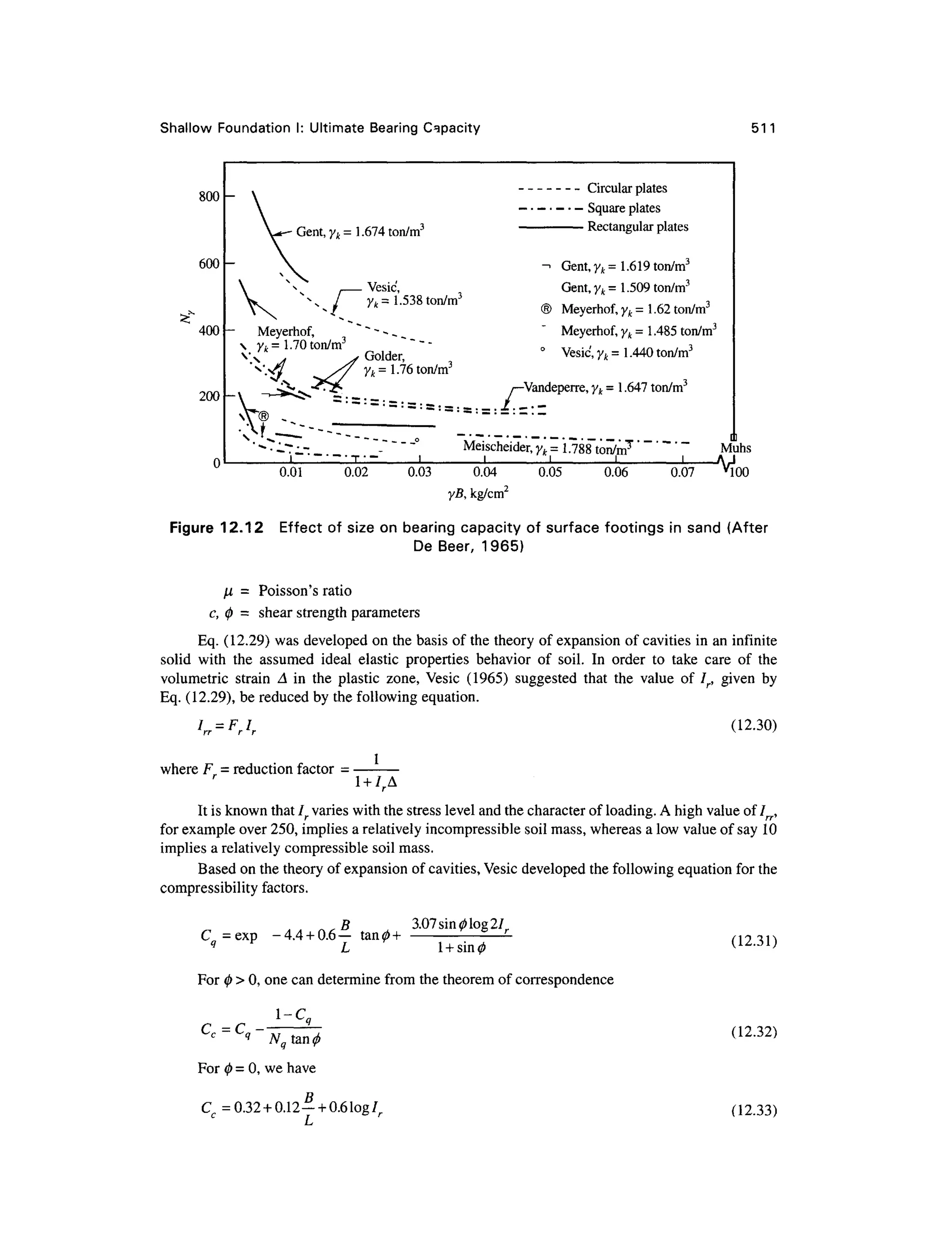
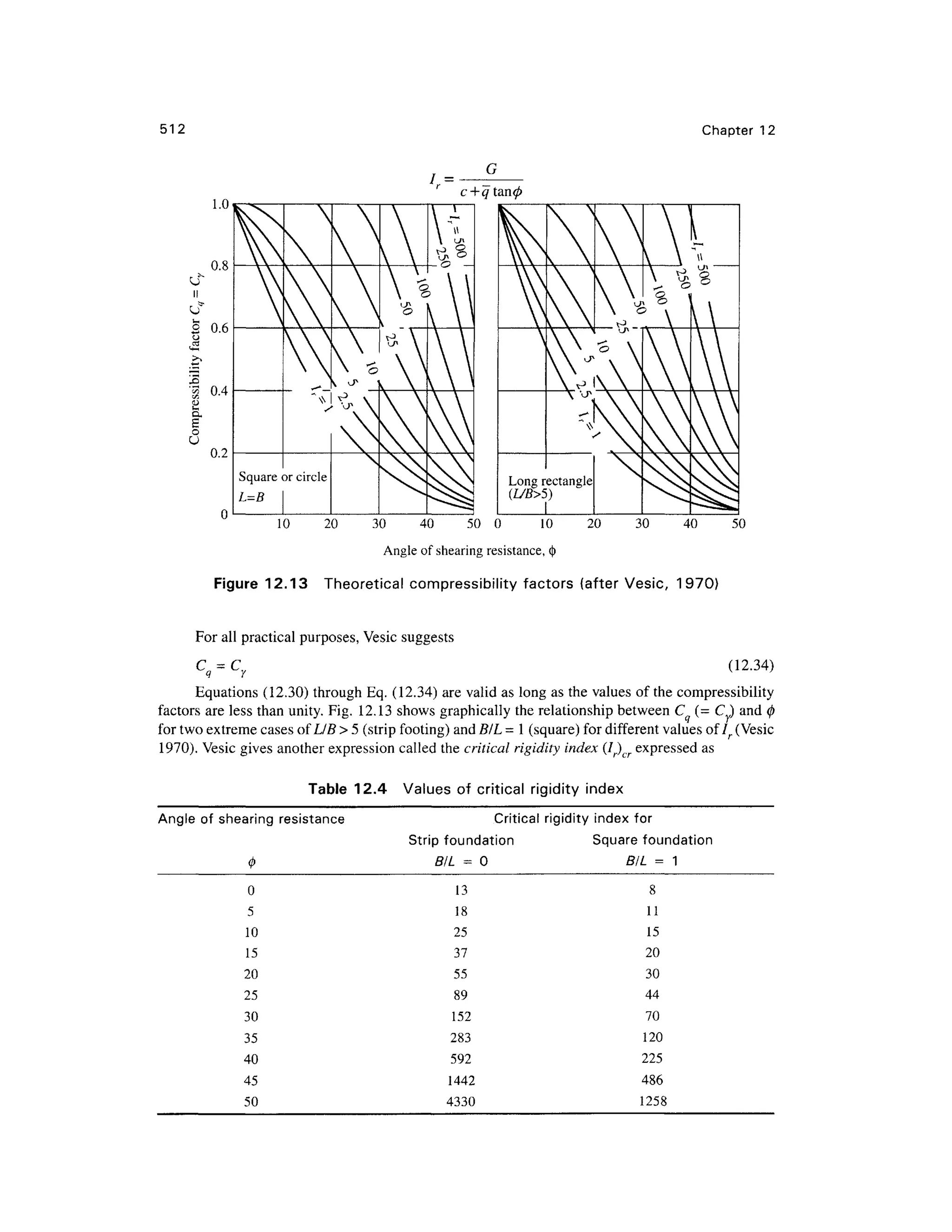
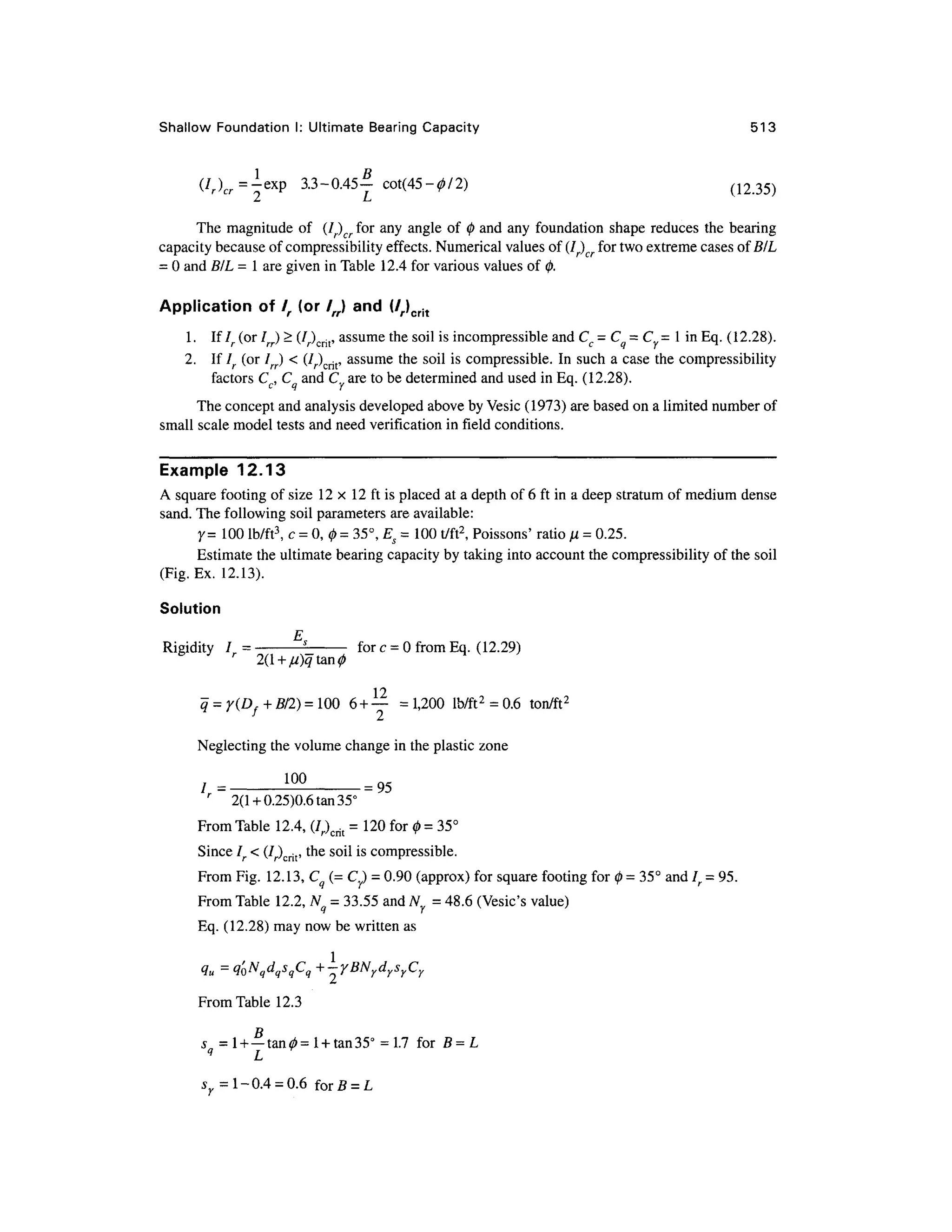
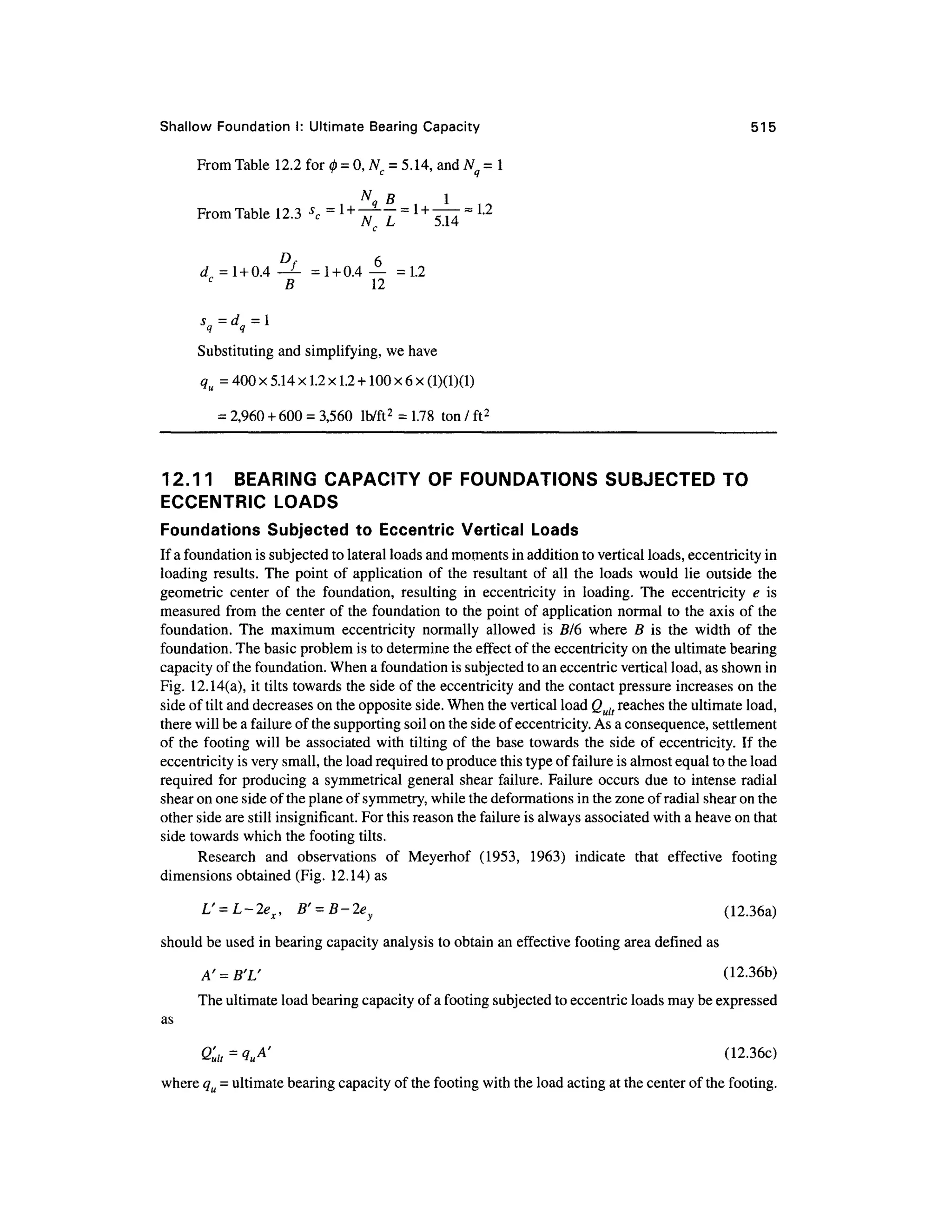
537. 518 Chapte r 1 2
When ex or e excee d a certain limit, Eq. (12.39) gives a negative value of q which indicates
tension between th e soil and the bottom of the footing. Eqs (12.39) ar e applicable onl y when the
load is applied within a limited area which is known as the Kern as is shown shaded in Fig 12.15 so
that the load may fall within the shaded area to avoid tension. The procedure for the determination
of soil pressur e whe n the load i s applied outside the kern is laborious and as such not dealt with
here. However, chart s are available for ready calculation s in references suc h as Teng (1969 ) an d
Highter and Anders (1985).
12.12 ULTIMAT E BEARIN G CAPACIT Y O F FOOTINGS BASE D O N
SPT VALUE S (N]
Standard Energ y Rati o Res Applicable to N Value
The effects of field procedures an d equipment on the field values of N were discussed in Chapter 9.
The empirical correlations establishe d in the USA between N and soil properties indicat e the value
of N conforms to certain standard energy ratios. Some suggest 70% (Bowles, 1996 ) and others 60%
(Terzaghi et al. , 1996) . I n order t o avoid this confusion, the autho r uses Ncor i n this book a s the
corrected value for standard energy.
Cohesionless Soil s
Relationship Betwee n Ncor and<| >
The relation between A^ and 0 established b y Peck e t al., (1974) is given in a graphical form in
Fig. 12.8 . The value ofNcor t o be used for getting 0 is the corrected valu e for standard energy. The
angle 0 obtained by this method can be used for obtaining the bearing capacity factors , and hence
the ultimate bearing capacity of soil.
Cohesive Soil s
Relationship Betwee n Ncor and qu (Unconfined Compressive Strength)
Relationships hav e been develope d betwee n Ncor an d qu (the undrained compressive strength ) for
the 0 = 0 condition . Thi s relationshi p give s th e valu e o f c u fo r an y know n valu e o f Ncor. Th e
relationship may be expressed a s [Eq. (9.12)]
tf^^jA^CkPa) (12-40 )
where the value of the coefficient& ma y vary from a minimum of 1 2 to a maximum of 25. A low
value of 1 3 yields qu given in Table 9.4 .
Once q u i s determined , th e ne t ultimat e bearing capacit y an d th e ne t allowabl e bearin g
pressure can be found following Skempton's approach.
12.13 TH E CR T METHO D O F DETERMINING ULTIMAT E BEARIN G
CAPACITY
Cohesionless Soil s
Relationship Between qc, Dr and 0
Relationships betwee n th e stati c con e penetratio n resistanc e q c an d 0 hav e bee n develope d b y
Robertson and Campanella (1983b) , Fig. 9.15. The value of $ can therefore be determined with the
known valu e of q . With the known value of 0 , bearing capacit y factor s ca n be determine d an d

538. Shallow Foundatio n I: Ultimate Bearin g Capacity 519
hence the ultimate bearing capacity. Experience indicates that the use of qc for obtaining 0 is more
reliable than the use of N.
Bearing Capacit y o f Soi l
As per Schmertmann (1978), the bearing capacity factors N an d N fo r use in the Terzaghi bearing
capacity equation can be determined by the use of the equation
N = (12.41)
where qc = cone point resistance in kg/cm2
(or tsf) averaged over a depth equal to the width below
the foundation.
Undrained Shea r Strengt h
The undrained shear strengt h cu under 0 = 0 condition ma y be related t o the stati c con e point
resistance qc as [Eq. (9.16)]
qc = N
kc
u+
Po
or c,, = (12.42)
where N k = con e factor , ma y b e take n a s equa l t o 2 0 (Sanglerat , 1972 ) bot h fo r normall y
consolidated an d preconsolidated clays .
po = tota l overburden pressure
When onc e c u i s known, the value s o f qm an d qna ca n b e evaluate d a s pe r th e method s
explained in earlier sections .
Example 12.1 5
A water tank foundation has a footing of size 6 x 6 m founded at a depth of 3 m below ground level
in a medium dense sand stratum of great depth. The corrected average SPT value obtained from the
site investigation is 20. The foundatio n is subjected to a vertical load a t an eccentricity o f fi/10
along one of the axes. Figure Ex. 12.15 gives the soil profile with the remaining data. Estimate the
ultimate load, Qult, by Meyerhof's method .
s/* //^
m
—1
QuU
^ €B -
SPT
c = 0,y=18.5kN/m3
,
0 = 33°, Ncor = 20
Medium dense san d
B
10
fix5 = 6 x 6m -H
Figure Ex. 12.1 5

539. 520 Chapte r 1 2
Solution
From Fig . 12.8 , 0=33° for N = 20.
e ' r
cor
B' = B-2e = 6- 2(0.6 ) -4.8 m
L' = L= B= 6m
For c = 0 and i = 1, Eq. (12.28) reduces to
From Table 12. 2 for 0 = 33° we have
Nq = 26.3, NY = 26.55 (Meyerhof )
From Tabl e 12. 3 (Meyerhof)
s = l +0.1Af — = l + 0.1tan2
45°+ — (1 ) =
1.34
q
* L 2
^=^=1.34 fo r 0> 10°
/ —D
f 3
d=l + Q.LN. -L
= 1 +0.1x1.84 — = 1.11 5
q V * B ' 4. 8
Substituting d y= dq = 1.1 15 fo r 0 > 10°
q'u = 18.5 x 3 x26.3 x1.34 x1.1 15 + -x 18.5 x 4.8 x26.55 x 1.34 x1.1 15
= 2,1 81+1,76 1=3,942 kN/m 2
Q'ult = BxB'xq' u = 6x4.8x3942= 113,53 0 kN-11 4 M N
Example 12.16
Figure Ex. 12.16 gives the plan of a footing subjected to eccentric loa d with two way eccentricity.
The footing is founded at a depth 3 m below the ground surface. Given ex =0.60 m and e = 0.75 m,
determine Q u[[. The soil properties are : c = 0, Ncgr = 20, y =18.5 kN/m3
. The soil is medium dense
sand. Use N(Meyerhof) fro m Table 12. 2 and Hansen's shape and depth factors from Table 12.3 .
Solution
Figure Ex . 12.1 6 show s th e two-wa y eccentricity . Th e effectiv e length s an d breadth s o f th e
foundation from Eq. (12.36a) is
B' = B-2e = 6- 2 x 0.75 = 4.5 m.
L' = L- 2e x = 6 - 2 x 0.6 =4.8 m.
Effective area , A' = L' x B' = 4.5 x 4.8 = 21.6 m2
As in Example 12.1 5

540. Shallow Foundatio n I: Ultimate Bearing Capacit y 521
6 m
ey = 0.75 m
e = 0.6 m
y
6 m -
Figure Ex . 12.16
For 0 = 33°, Nq = 26.3 and Ny = 26.55 (Meyerhof)
From Table 12. 3 (Hansen)
B' 4 5
5 = 1 + —tan33° = l +—x 0.65 = 1.61
q
L ' 4. 8
R' 4 5
sv =1-0.4—=1-0.4 x— = 0.63
Y
L' 4. 8
da = l + 2tan33°(l-sin33°)2
x —
* 4. 5
= 1 + 1.3x0.21x0.67 =1.183
Substituting
1
q'u = 18.5x3x26.3xl.61xl.l83+-xl8.5x4.5x26.55x0.63x(l )
= 2,780 + 696 = 3,476 kN/m 2
Quh = A'q'u = 21.6 x3,476 = 75,082 k N
12.14 ULTIMAT E BEARIN G CAPACITY O F FOOTINGS RESTIN G
ON STRATIFIE D DEPOSIT S O F SOIL
All the theoretical analysis dealt with so far is based on the assumption that the subsoil is isotropic
and homogeneou s t o a considerable depth . In nature , soil i s generall y non-homogeneou s with
mixtures of sand, silt and clay in different proportions . In the analysis, an average profile of such
soils is normally considered. However, if soils are found in distinct layers of different composition s
and strength characteristics, the assumption of homogeneity to such soils is not strictly valid if the
failure surface cuts across boundaries of such layers.

541. 522 Chapte r 1 2
The present analysis is limited to a system of two distinct soil layers. For a footing located in
the upper layer at a depth D, below the ground level, the failure surfaces at ultimate load may either
lie completely i n the uppe r layer or may cross the boundary o f the two layers . Further , w e may
come across the upper layer strong and the lower layer weak or vice versa . In either case, a general
analysis for (c - 0 ) will be presented and will show the same analysis holds true if the soil layers are
any one of the categories belongin g to sand or clay.
The bearin g capacit y o f a layere d syste m wa s firs t analyze d b y Butto n (1953 ) wh o
considered onl y saturate d cla y ( 0 = 0). Later o n Brown an d Meyerho f (1969 ) showe d tha t th e
analysis o f Butto n lead s t o unsaf e results . Vesic (1975 ) analyze d th e tes t result s o f Brow n an d
Meyerhof an d others an d gave his own solution to the problem .
Vesic considered bot h the types of soil in each layer, that is clay and (c - 0 ) soils. However ,
confirmations of the validity of the analysis of Vesic and others are not available. Meyerhof (1974 )
analyzed the two layer system consisting of dense sand on soft clay and loose sand on stiff clay and
supported hi s analysi s with som e mode l tests . Again Meyerho f an d Hanna (1978 ) advanced th e
earlier analysi s o f Meyerhof (1974 ) to encompass ( c - 0 ) soil an d supported thei r analysis with
model tests. The present section deals briefly wit h the analyses of Meyerhof (1974 ) and Meyerhof
and Hanna (1978) .
Case 1 : A Stronge r Laye r Overlyin g a Weaker Deposi t
Figure 12.16(a ) shows a strip footing of width B resting at a depth D, below groun d surfac e in a
strong soil layer (Layer 1) . The depth to the boundary of the weak layer (Layer 2) below the base of
the footing is H. If this depth H is insufficient to form a full failure plastic zone in Layer 1 under the
ultimate load conditions, a part of this ultimate load will be transferred t o the boundary leve l mn.
This load will induce a failure condition in the weaker layer (Layer 2). However, if the depth H is
relatively larg e the n th e failur e surfac e wil l b e completel y locate d i n Laye r 1 a s show n i n
Fig. 12.16b .
The ultimate bearing capacities of strip footings on the surfaces of homogeneous thic k beds
of Layer 1 and Layer 2 may be expressed a s
Layer 1
q=c
N
c+
-YBN
r (12.43 )
Layer 2
1 „. ,
Ny2 (12.44 )
where Ncl, N . - bearin g capacity factors for soil in Layer 1 for friction angle 0 j
Nc2, Ny2 = bearing capacity factors for soil in Layer 2 for friction angl e 02
For th e footing founded at a depth ZX , if the complete failur e surface lie s within the upper
stronger Layer 1 (Fig. 12.16(b) ) an expression for ultimate bearing capacity of the upper layer may
be written as
qu = v< =c
iN
ci+
VoN
qi+
^riBN
n (12.45 )
If q is much greate r that q2 and if the depth H is insufficient t o form a full failur e plasti c
condition in Layer 1 , then the failure of the footing may be considered du e to pushing of soil within
the boundary ad and be through the top layer into the weak layer. The resisting force for punching
may be assumed t o develop o n the faces ad and be passing throug h the edges of the footing. The
forces that act on these surfaces are (per unit length of footing),

542. Shallow Foundatio n I : Ultimate Bearin g Capacit y 523
^ f <*^<*r^<0^
D
f
1
,
Q
.t
?«
1
,
,
a b
^^^^^^^^
ca
i Laye r 1 : stn
. X i
H
Layer 2: weaker y 2> 02'C
2
(b)
Figure 12.1 6 Failur e of soi l belo w stri p footing under vertica l loa d on strong layer
overlying wea k deposi t (afte r Meyerhof an d Hanna, 1978 )
Adhesive force, C a =caH
Frictional force, F, = P si n (12.46)
where ca = unit cohesion, P - passiv e earth pressure per unit length of footing, and<5 = inclination
of Pp with the normal (Fig 12.16(a)) .
The equation for the ultimate bearing capacity qu for the two layer soil system may now be
expressed as
2(Ca+P sin<5 )
•q = q.+ -
a
- -
p
~ -- yH
"u "b T) ' I
where, qb - ultimat e bearing capacity of Layer 2
The equation for P ma y be written as
(12.47)
H (12.48)

543. 524 Chapter 1 2
40
35
30
25
^--J
I 2 0
i15
u
10
Approx. bearing
capacity rati o
0.4
0.2
0
20° 25 ° 30 ° 35 ° 40 ° 45 ° 50 °
0i (deg)
Figure 12.1 7 Coefficient s of punchin g shea r resistance under vertica l loa d (after
Meyerhof an d Hanna, 1978 )
1.0
0.9
§ 0. 7
CU
0.6
0.2 0. 4 0. 6 0. 8
Bearing capacit y rati o q~Llql
1.0
Figure 12.1 8 Plo t o f ca/c1 versus q2lq^ (afte r Meyerho f an d Hanna, 1978 )

544. Shallow Foundatio n I : Ultimate Bearin g Capacit y 52 5
Substituting for P an d Ca, the equation for qu may be written as
2caH r^H 2 2D
f
^=^+
-|- +
-y
- 1 +
-^
- KptanS-r,H (1249 )
In practice, i t is convenient to use a coefficient K s o f punching shearing resistanc e o n th e
vertical plane through the footing edges so that
Ks tan ^= Kp ta n 8 (12.50 )
Substituting, the equation for qu may be written as
2cH ,H 2
2D
Figure 12.17 gives the value of Ks for various values of 0j as afunction of <?2/gr The variation
i with q^ql i s shown in Fig. 12.18.
Equation (12.45 ) for qt an d qb in Eq. (12.51 ) ar e for strip footings. These equations wit h
shape factors may be written as
-Y,BNnsn (12.52 )
,2 +Y2BN
Y2s
n. (12.53 )
where sc, s an d s ar e th e shap e factor s fo r th e correspondin g layer s wit h subscript s 1 and 2
representing layers 1 and 2 respectively.
Eq. (12.51) can be extended to rectangular foundations by including the corresponding shape
factors.
The equation for a rectangular footing may be written as
2c H B Y<H 2
2D , B
4u=<lb+ ~
1 + Y +-y - l + -
~ 'l + -
Case 2 : To p Layer Dens e Sand and Bottom Layer Saturate d Soft Cla y (02 = 0 )
The value of qb for the bottom layer from Eq. (12.53) may be expressed a s
^b=C
2N
c2S
c2+
r^D
f+H
'> (12-55 )
From Table (12.3), sc2 = (1+0.2 B/L) (Meyerhof , 1963 ) and Nc = 5.14
for 0 = 0. Therefore
qb= 1 + 0.2- 5.Uc 2+ri(Df+H) (12 .56)
LJ
For C j = 0, q t from Eq. (12.52) is
<?, = r^/^V,
! +
riBN
ns
n (12-57 )

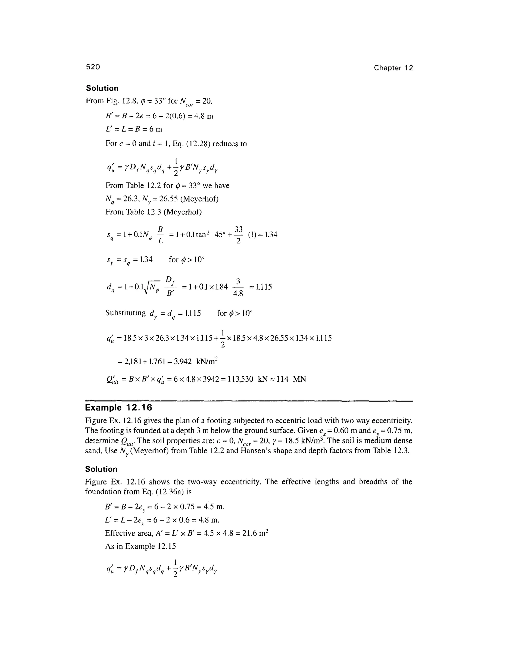
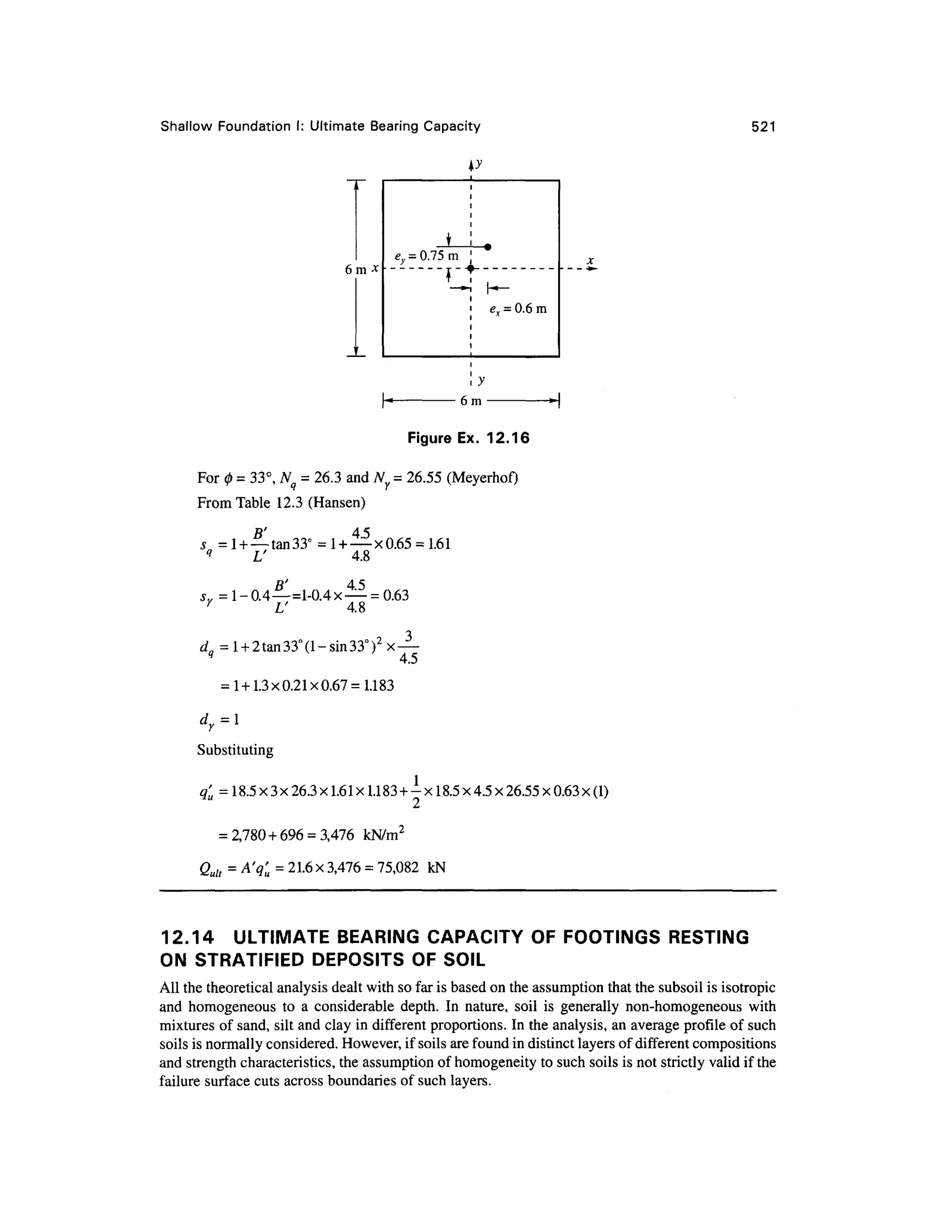
545. 526 Chapte r 1 2
We may now write an expression for qu from Eq . (12.54) as
B y,H 2
2D f B
q = 1 + 0.2— 5.14c ?+^ -
1+ — Li + _K tan0 ,
" L 2
B H L s l
+ ylDf<y]DfNqlS(il+~ylBNrlsn (12.58 )
The ratio of q1lql ma y be expressed by
C
^ 5.14 c
The value of Ks ma y be found fro m Fig. (12. 17).
Case 3 : Whe n Laye r 1 is Dense Sand and Layer 2 is Loose Sand (c 1 = c 2 = 0 )
Proceeding i n the same way as explained earlier the expression for qu for a rectangular footing may
be expressed as
qu= Y, f
y.H2
B 2 D
- ~ (1260)
where q t = Y^f^s^ +-Y^BN nsn (12.61 )
<12
-62)
Case 4 : Laye r 1 is Stiff Saturate d Cla y (01 = 0 ) an d Layer 2 i s Saturated Sof t
Clay (0 2 = 0 )
The ultimate bearing capacity of the layered system can be given as
qu= 1 + 0.2-5.Uc 2+ 1 + | ^- + y
]Df<qt (12 .63)
D
q,= 1 + 0.2
- 5.14c,+y,D / (12.64 )
L
q2 _ 5.1 4 c2 _
(12.65)
Example 12.1 7
.
A rectangular footing of size 3 x 2 m is founded at a depth of 1. 5 m in a clay stratum of very stif f
consistency. A clay laye r of medium consistency is located a t a depth o f 1. 5 m ( = H) belo w th e
bottom of the footing (Fig. Ex. 12.17) . The soil parameters of the two clay layers are as follows:
Top clay layer: c = 175 kN/m2

546. Shallow Foundatio n I : Ultimate Bearin g Capacity 527
;^:v4^>-i;y^v---f-
Df= 1.5m"' '
:
''V'y'i''v^-.'-V'' '•':'*i.;':
-:
''.;
•..' Ver y stiff clay
Soft clay
Layer 2 c 2 = 40 kN/m2
y2 = 17.0 kN/m3
Figure Ex. 12.1
7
7t = 17.5 kN/m3
Bottom layer: c 2 = 40 kN/m2
y2 = 17.0 kN/m3
Estimate the ultimate bearing capacity and the allowable bearing pressure on the footing with
a factor of safety of 3.
Solution
The solutio n t o thi s proble m come s unde r Case 4 i n Sectio n 12.14 . W e have t o conside r her e
Eqs (12.63), (12.64 ) an d (12.65).
The data given are:
fl = 2m,L = 3m, H= 1.5m (Fig. 12.16a),D/= 1.5m, ^ = 17.5 kN/m
3
.
From Fig. 12.18, for q2lql = c2/cl = 40/175 = 0.23,
the value of cjcl = 0.83 or ca = 0.83^ = 0.83 x175 =145.25 kN/m 2
.
From Eq. (12.63 )
B B 2 c H
q = 1 + 0.2— 5.14c ~ + 1 + — -^— + y,Df<q,
u
L L B }
Substituting the known values
2xl45
-25x1
-5
q = 1 + 0.2X- 5.14x40 + 1 + -
y
" 3 3
+n.5xl.5
= 233 + 364 + 26 = 623 kN/m 2

547. 528 Chapte r 1 2
FromEq. (12.64)
D
qt = 1 + 0.2— 5.14c , + y}Df
= l + 0.2x- 5.14x17 5 + 17.5x1.5
3
-1020 + 26-1046 kN/m 2
It is clear fro m the above that qu < q( an d as such qu is the ultimate bearing capacity to be
considered. Therefor e
kN/m2
Example 12.1 8
Determine the ultimate bearing capacity of the footing given in Example 12.1 7 in dense sand with
the bottom layer being a clay of medium consistency. The parameters of the top layer are:
/! = 18. 5kN/m3
, 0j = 39°
All the other data given in Ex. 12.17 remain the same. Use Meyerhof's bearing capacity and
shape factors.
Solution
Case 2 of Section 12.1 4 is required to be considered here.
Given: Top layer: y, = 18.5 kN/m3
, 01 = 39°, Bottom layer: y2 = 17.0 kN/m3
, c2 = 40 kN/m2
.
From Table 12. 2 Nyl (M) = 78.8 for 0j = 39°.
FromEq. (12.59)
<? 5.14 c 5.14x4 0
ql (XSj^flA fj 0.5x18.5x2x78. 8
From Fig. 12.1 7 Ks = 2.9 for 0 = 39°
Now from Eq . (12.58) we have
B y H 2
2 D B
q - 1 + 0.2— 5.14c , +— 1 + —
- 1 + —K
L 2
B H L *
7 1 8 S v n 5^ 7 x 1 ^ 7
= 1 + 0.2X- 5.14x40 + V ;
+ =——1 + -
2.9tan39°+18.5x1.5
3 2 1. 5 3
-233 +245 +28 = 506 kN/m 2
qu - 506 kN/m2
From Eq. (12.58) the limiting value qt is
qt =

548. Shallow Foundatio n I: Ultimate Bearing Capacity 52 9
where ^ = 18.5 kN/m3
, Df= 1.5m , B = 2 m.
From Table 12. 2 Nyl = 78.8 and Nql = 56.5
B 3 9 2
From Table 12. 3 ^ =1 +0.1
^ — =l + 0.1xtan2
45°+ — x - = l29 = syl
/_> £ J
Now <? r = 18.5 x 1.5 x56.5 x1.29 +-
x 18.5 x 2x78.8 x1.29 = 3903 kN/m 2
> qu
Hence<= 506 kN/m 2
12.15 BEARIN G CAPACIT Y OF FOUNDATIONS ON TO P O F A
SLOPE
There are occasions where structures are required to be built on slopes or near the edges of slopes.
Since full formations of shear zones under ultimate loading conditions are not possible on the sides
close to the slopes or edges, the supporting capacity of soil on that side get considerably reduced.
Meyerhof (1957 ) extende d hi s theorie s t o includ e th e effec t o f slope s o n th e stabilit y o f
foundations.
Figure 12.1 9 shows a section of a foundation with the failure surfaces under ultimate loading
condition. The stability of the foundation depends on the distance b of the top edge of the slop e
from th e face of the foundation.
The for m o f ultimat e bearing capacit y equatio n fo r a stri p footin g ma y b e expresse d a s
(Meyerhof, 1957 )
1
(12.66)
The uppe r limi t of the bearing capacit y o f a foundation in a purely cohesive soi l ma y b e
estimated fro m
qu = cN c +yD f (12.67 )
The resultan t bearing capacit y factors Ncq an d N depen d on the distance b » A 0 an
d th e
DJB ratio. These bearing capacity factors are given in Figs 12.2 0 and 12.2 1 for strip foundation in
purely cohesive and cohesionless soils respectively. It can be seen from the figures that the bearing
capacity factors increase with an increase of the distance b • Beyond a distance of about 2 to 6 times
the foundatio n width B, th e bearing capacit y is independent of the inclination of the slope , an d
becomes the same as that of a foundation on an extensive horizontal surface.
For a surcharg e ove r th e entir e horizonta l to p surfac e o f a slope , a solutio n o f th e slop e
stability has been obtained on the basis of dimensionless parameters called the stability number Ns,
expressed as
NS
=^H (12
-68)
The bearin g capacit y o f a foundatio n o n purel y cohesiv e soi l o f grea t dept h ca n b e
represented by Eq. (12.67) where the Nc facto r depends on b a s well as ft, and the stability number
N. Thi s bearin g capacit y factor , whic h i s give n i n th e lowe r part s o f Fig . 12.20 , decreas e
considerably wit h greater heigh t and to a smaller exten t with the inclination of the slope. For a
given heigh t and slope angle , th e bearing capacit y facto r increase s wit h an increase i n b . an
d

549. 530 Chapter 1 2
90°-
Figure 12.1 9 Bearin g capacity o f a strip footing on top o f a slope (Meyerhof ,
1957)
beyond a distance of about 2 to 4 times the height of the slope, the bearing capacity is independent
of the slope angle. Figure 12.2 0 shows that the bearing capacity of foundations on top of a slope is
governed b y foundatio n failure fo r smal l slop e heigh t (A ^ approachin g infinity ) an d b y overal l
slope failure for greater heights.
The influenc e of ground water and tension cracks (i n purely cohesive soils ) should also be
taken into account i n the study of the overall stability of the foundation .
Meyerhof (1957 ) has not supported his theory with any practical examples of failure as any
published data were not available for this purpose.
Bearing
capacity
factor
N
cq
*—
•
t
O
U
>
-P
^
Lf
i
O
N
-~
J
O
_
X
7-f
30^
"60°
i?
/ j
<r/
30V
/
/
A!
-30°
Incli
si
0°
10°'
X
X
)0
PS.'
, .S'
'/
/
°/
/
^°:
^90
natio
ope/
X
•9-- '
''6C
/•
/
^
<f
/
/
90°
^
D
/
/ 0°
/I
^
f~^'
_9
/
/*
n of
3
-'_
X
9
/
'
f
^
^
X"
3° '
/
^
s^-
^
''
s
s
s
^^"^
<*>***
,
'
,'"
SI
" >
W,=
ope stabil
factor yv s
/co
0.5
j
r
/0.25
yO.18
S
- 0 0
ity
Foundation depth/width
Df/B = 0
Df/B=l
0 1 2 3 4 5 6
Distance of foundation fro m edg e of slope b/B
Figure 12.2 0 Bearin g capacity factor s for stri p foundation on top o f slop e of
purely cohesiv e materia l (Meyerhof , 1957 )

550. Shallow Foundatio n I : Ultimate Bearin g Capacit y 531
400
300
200
100
50
25
10
,'"
X
'.-•
A
/
/
II
X
^•0°
^*
^
30U
£^1
iclin
slo
20
"'
atior
pe^
3°
r'
40 V
x I
^^
90
^-*-
of
^* *
**•"**
^--
^ —
^-*^
_ — -
F
£
£
L
ii
Ang
„--
^=
— ~ "
oundation depth/width
fit) — U
) / D 1
/•//5 — 1
inear inte
itermedia
leof
Ticti<
j
„ - -
40°
^=^
30
*
30
intei
Dn 0
f
_ -
^^
rpolation for
te depths
nal
0 1 2 3 4 5 6
Distance of foundation fro m edg e of slope b/B
Figure 12.21 Bearin g capacity factors for stri p foundation o n top o f slop e of
cohesionless materia l (Meyerhof , 1957 )
Example 12.1 9
A strip footing is to be constructed on the top of a slope as per Fig. 12.19 . The following data are
available:
B = 3m,Df= 1.5m , b = 2m, H=8 m, p=30°, y= 18.5 kN/m3
, 0 = 0 and c = 75 kN/m2
,
Determine the ultimate bearing capacity of the footing.
Solution
PerEq. (12.67) qu for 0 = 0 is
From Eq. (12.68)
c 15
yH 18.5x 8
= 0.51
and — = — =0.
From Fig. 12.20 , N = 3.4 for N = 0.51 , A/f i = 0.67, an d j8= 30°
D ' C q $ ' c /•" r~
Therefore
a = 75 x 3.4 + 18.5 x 1. 5 = 255+28 = 283 kN/m2
.

551. 532 Chapte r 1 2
12.16 FOUNDATION S O N ROC K
Rocks encountere d i n nature might be igneous, sedimentary or metamorphic. Granit e and basalt
belong t o the first group . Granite is primarily composed o f feldspar, quartz and mica possesses a
massive structure . Basal t i s a dark-colore d fin e graine d rock . Bot h basal t an d granit e unde r
unweathered condition s serv e a s a ver y goo d foundatio n base. Th e mos t importan t rock s tha t
belong to the second group are sandstones, limestones and shales. These rocks are easily weathered
under hostile environmental conditions and arsuch, the assessment o f bearing capacity o f these
types requires a little care. In the last group come gneiss, schist, slate and marble. Of these rock s
gneiss serves as a good bearing material whereas schist and slate possess poor bearing quality.
All rocks weather under hostile environments. The ones that are close to the ground surface
become weathered mor e than the deeper ones. If a rocky stratum is suspected close to the ground
surface, the soundness or otherwise of these rocks must be investigated. The quality of the rocks is
normally designated by RQD as explained in Chapter 9.
Joints are common in all rock masses. This word joint is used by geologists fo r any plane of
structural weakness apart from faults within the mass. Within the sedimentary rock mass the joints
are lateral in extent and form what are called bedding planes, and they are uniform throughout any
one be d withi n igneous roc k mass . Coolin g joint s ar e mor e closel y space d neare r th e groun d
surface with wider spacings at deeper depths. Tension joints and tectonic joints might be expecte d
to continu e depth wise . Withi n metamorphi c masses , ope n cleavage , ope n schistos e an d ope n
gneissose plane s ca n b e o f considerabl y furthe r latera l exten t tha n th e beddin g plane s o f th e
sedimentary masses .
Faults an d fissure s happe n i n roc k masse s du e t o interna l disturbances . Th e joint s wit h
fissures and faults reduces the bearing strength of rocky strata.
Since mos t unweathere d intact rocks ar e stronger an d less compressibl e tha n concrete, th e
determination o f bearin g pressure s o n suc h material s ma y no t b e necessary . A confine d roc k
possesses greater bearing strength than the rocks exposed at ground level.
Bearing Capacit y o f Rock s
Bearing capacities of rocks are often determine d by crushing a core sample in a testing machine.
Samples used for testing must be free from cracks and defects.
In the rock formation wher e bedding planes, joints and other planes o f weakness exist, the
practice tha t i s normall y followe d i s t o classif y th e roc k accordin g t o RQ D (Roc k Qualit y
Designation). Table 9.2 gives the classification of the bearing capacity of rock according to RQD
.
Peck et al, (1974) have related the RQD to the allowable bearing pressure qa as given in Table 12.5
The RQD for use in Table 12. 5 should be the average within a depth below foundation level
equal to the width of the foundation, provided the RQD is fairly uniform within that depth. If the
upper part of the rock, within a depth of about 5/4, is of lower quality, the value of this part should
be used.
Table 12. 5 Allowabl e Bearin g Pressure q o n Jointed Rock
RQD
100
90
75
50
25
0
qg Ton/ft 2
300
200
120
65
30
10
qg MP a
29
19
12
6.25
3
0.96

552. Shallow Foundatio n I: Ultimate Bearing Capacity 533
Table 12. 6 Presumptiv e allowabl e bearin g pressures on rock s (MPa ) as
recommended b y various building codes in USA (after Peck et al., 1974 )
Rock type Building Codes
BOCA Nationa l Unifor m LO S Angeles
(1968) (1967 ) (1964 ) (1959 )
1. Massive crystalline bedrock,
including granite diorite, gneiss, 1 0
basalt, hard limestone and dolomite
2. Foliated rocks such as schist or
slate in sound condition 4
3. Bedded limestone in sound condition
sedimentary rocks including hard 2. 5
shales and sandstones
4. Soft o r broken bedrock
10 0.2 q*
1.5 0-29.
1.0
0.4
0.3
(excluding shale) and sof t
limestone
5. Soft shale
1.0
0.4
0.2 qu
0.2 qu
* q = unconfined compressive strength.
Another practic e tha t i s normall y followe d i s t o bas e th e allowabl e pressur e o n th e
unconfined compressive strength, qu, of the rock obtained in a laboratory on a rock sample. A factor
of safety of 5 to 8 is used on qu to obtain qa. Past experience indicates that this method is satisfactory
so long as the rocks in situ do not possess extensive cracks and joints. In such cases a higher factor
of safety may have to be adopted.
If rock s clos e t o a foundatio n base ar e highl y fissured/fractured , they ca n b e treate d b y
grouting which increases the bearing capacity of the material.
The bearing capacity of a homogeneous, and discontinuous rock mass cannot be less than the
unconfined compressiv e strengt h of the rock mass around the footing and this can be taken as a
lower bound for a rock mass with constant angle of internal friction 0 and unconfined compressive
strength qur. Goodman (1980) suggests the following equation for determining the ultimate bearing
capacity qu.
(12.69)
whereA f = tan2
(45° + 0/2), q ur = unconfined compressive strengt h of rock.
Recommendations b y Buildin g Code s
Where bedroc k ca n b e reache d b y excavation , th e presumptiv e allowabl e bearin g pressur e i s
specified by Building Codes. Table 12.7 gives the recommendations of some buildings codes in the
U.S.
12.17 CAS E HISTORY O F FAILURE OF THE TRANSCON A
GRAIN ELEVATOR
One o f th e bes t know n foundatio n failure s occurre d i n Octobe r 191 3 a t Nort h Transcona ,
Manitoba, Canada . I t wa s ascertaine d late r o n tha t th e failur e occurred whe n th e foundation

553. 534 Chapte r 1 2
Figure 12.2 2 Th e tilted Transcona grai n elevator (Courtesy: UMA Engineering
Ltd., Manitoba , Canada )
Figure 12.2 3 Th e straightened Transcona grain elevator (Courtesy : UM A
Engineering Ltd. , Manitoba , Canada )

554. Shallow Foundatio n I: Ultimate Bearin g Capacit y 535
Ground leve l
Organi clay fill
and silty caly
Varved brown clay
with horizontal strati-
fication
Greyish silty
clay with
calcareous sil t
Grey silt y clay with
calcareous silt pocket s
Silty gravel
770
760
750
740
730
720
Refusal
(a) Classification fro m
test boring
0 1. 0 2. 0 3. 0
Unconfmed compressive strengt h (TSF )
(b) Variation of unconfmed compressiv e
strength with depth
Figure 12.2 4 Result s of test borin g a t site of Transcon a grain elevato r (Pec k and
Byrant, 1953 )
pressure a t the base was about equal to the calculated ultimate bearing capacity of an underlaying
layer of plastic clay (Peck and Byrant,1953), and was essentially a shearing failure.
The construction of the silo started i n 191 1 and was completed i n the autumn of 1913 . The
silo is 77 ft by 19 5 ft in plan and has a capacity of 1,000,000 bushels. It comprises 6 5 circular bins
and 48 inter-bins. The foundation was a reinforced concrete raft 2 ft thick and founded at a depth of
12 ft below the ground surface. The weight of the silo was 20,000 tons, which was 42.5 percent of
the total weight, when it was filled. Filling the silo wit h grain started i n September 1913 , and in
October when the silo contained 875,000 bushels, and the pressure on the ground was 94 percent of
the design pressure, a vertical settlement of 1 ft was noticed. The structure began to tilt to the west
and within twenty four hours was at an angle of 26.9° fro m th e vertical, the west side being 24 ft
below an d th e eas t sid e 5 f t abov e th e origina l leve l (Szechy , 1961) . Th e structur e tilte d a s a
monolith and there was no damage to the structure except for a few superficial cracks. Figure 12.2 2
shows a view of the tilted structure . The excellent qualit y of the reinforced concret e structur e is
shown by the fact that later it was underpinned and jacked u p on new piers founded on rock. The

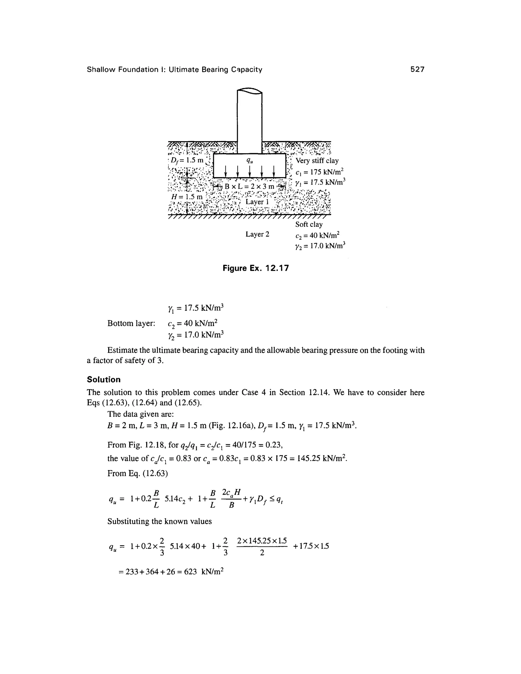
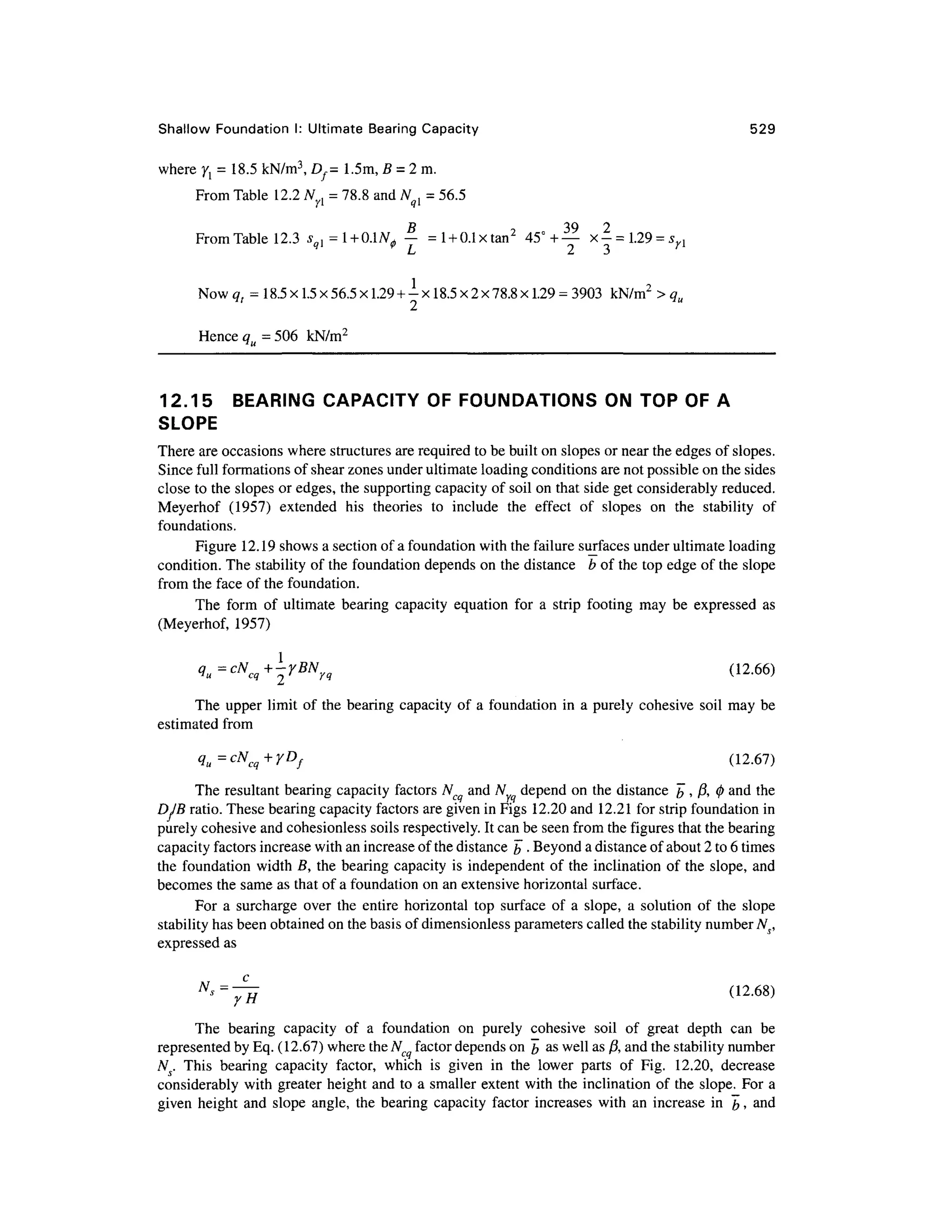
555. 536 Chapter 1 2
level of the new foundation is 34 ft below th e ground surface. Figure 12.2 3 shows the view of the
silo after it was straightened in 1916 .
During the period whe n the silo was designed and constructed, soil mechanics as a scienc e
had hardly begun. The behavior of the foundation under imposed loads was not clearly understood.
It was only during the year 1952 that soil investigation was carried out close to the silo and the soil
properties were analyze d (Peck an d Byrant, 1953) . Figure 12.2 4 give s the soi l classificatio n and
unconfmed compressiv e strengt h o f th e soi l wit h respec t t o depth . Fro m th e examinatio n o f
undisturbed sample s o f th e clay, it was determined tha t the averag e wate r content o f successiv e
layers of varved clay increased wit h their depth from 40 percent to about 60 percent. The average
unconfmed compressive strength of the upper stratum beneath th e foundation was 1.1 3 tsf, that of
the lower stratum was 0.65 tsf, and the weighted average was 0.93 tsf. The average liquid limit was
found to be 105 percent; therefore the plasticity index was 70 percent, which indicates that the clay
was highly colloidal an d plastic. The average unit weight of the soil was 12 0 lb/ft3
.
The contact pressure due to the load from the silo at the time of failure was estimated as equal to
3.06 tsf. The theoretical values of the ultimate bearing capacity by various methods are as follows.
Methods a., tsf
Terzaghi[Eq. (12.19)]
Meyerhof [Eq . (12.27)]
Skempton [Eq . (12.22)]
3.68
3.30
3.32
The above values compare reasonabl y well with the actual failure load 3.0 6 tsf . Perloff and
Baron (1976) give details of failure of the Transcona grain elevator.
12.18 PROBLEM S
12.1 Wha t will be the gross and net allowable bearing pressures of a sand having 0 = 35° and an
effective uni t weight of 1 8 kN/m3
under the following cases: (a) size of footing 1 x 1 m
square, (b ) circular footing of 1 m dia., and (c) 1 m wide strip footing.
The footing is placed at a depth of 1 m below the ground surface and the water table is at
great depth. Use F^ = 3. Compute by Terzaghi's genera l shear failure theory.
1 m :
Sand ••'•:
.•...;•-.;..• y = 1 8 kN/m3
12.2 A strip footing is founded at a depth of 1. 5 m below the ground surface (Fig. Prob. 12.2) .
The wate r tabl e i s clos e t o groun d leve l an d th e soi l i s cohesionless . Th e footin g i s
supposed to carry a net safe load of 400 kN/m2
with F = 3. Given y= 20.85 kN/m3
and

556. Shallow Foundatio n I: Ultimate Bearin g Capacity 537
0 = 35°, fin d th e require d widt h of th e footing , using Terzaghi's genera l shea r failure
criterion.
.' '•..';:. ' San d
1.5m • •' •• ' •'• •
I i i
•-'v':.- 0 = 35°
;';;.•' y sat = 20.85 kN/m3
i i I
Figure Prob . 12. 2
12,3 A t what depth should a footing of size 2 x 3 m be founded to provide a factor of safety of 3
if the soil is stiff clay having an unconfined compressive strength of 12 0 kN/m2
? The unit
weight of the soil is 18 kN/m3
. The ultimate bearing capacity of the footing is 425 kN/m2
.
Use Terzaghi's theory. The water table is close to the ground surface (Fig. Prob. 12.3) .
Dt=l
Stiff clay
qu = 120 kN/m2
y= 1 8 kN/m3
0 = 0
B xL = 2 x 3m *- |
Figure Prob. 12. 3
12.4 A rectangular footing is founded at a depth of 2 m below the ground surface in a (c -0 ) soil
having the following properties: porosity n = 40%, Gs =2.67, c = 15 kN/m2
, and 0 = 30°.
The water table is close to the ground surface. If the width of the footing is 3 m, what is the
length required to carry a gross allowable bearing pressure qa = 455 kN/m2
with a factor of
safety = 3? Use Terzaghi's theory of general shear failure (Figure Prob. 12.4).

557. 538 Chapter 1 2
V
n 9 m
L)f z m
1
#J
1 1
n = 40%
G, = 2.67
1 c
= 15kN/ m
(jj -30
h- Bx L = 3xL - H
Figure Prob. 12.4
12.5 A square footing located a t a depth of 5 ft below the ground surface in a cohesionless soil
carries a column load of 130 tons. The soil is submerged having an effective unit weight of
73 lb/ft3
an d an angle of shearing resistance o f 30°. Determin e th e size of the footing for
F = 3 by Terzaghi's theory of general shear failure (Fig. Prob. 12.5) .
D/=5ft;
i I 1
' San d
1
1
;: y b = 73 lb/ft 3
;• '0 = 30 °
|-« B x B ^
Figure Prob . 12. 5
12.6 A footin g o f 5 f t diamete r carrie s a saf e loa d (includin g it s sel f weight ) o f 8 0 ton s i n
cohesionless soi l (Fig. Prob. 12.6). The soil has an angle of shearing resistance</ > = 36° an d
an effective unit weight of 80 lb/ft3
. Determine the depth of the foundation for Fs = 2.5 by
Terzaghi's genera l shear failure theory.
£>,=
i I i. •
80 ton
yh = 80 lb/ft3
0 = 36°
5ft
Figure Prob . 12. 6

558. Shallow Foundatio n I : Ultimate Bearin g Capacit y 539
12.7 I f the ultimate bearing capacity of a 4 ft wide strip footing resting on the surface of a sand
is 5,25 0 lb/ft2
, wha t will be th e ne t allowabl e pressur e tha t a 1 0 x 1 0 ft squar e footing
resting o n th e surfac e can carr y wit h FS = 37 Assume that the soi l i s cohesionless. Us e
Terzaghi's theory of general shear failure.
12.8 A circular plate of diameter 1.05 m was placed on a sand surface of unit weight 16.5 kN/m3
and loade d t o failure . The failur e load wa s foun d to giv e a pressur e o f 1,50 0 kN/m 2
.
Determine the value of the bearing capacity factor N . The angle of shearing resistance of
the san d measure d i n a triaxial test wa s found to be 39° . Compar e thi s valu e with the
theoretical value of N . Use Terzaghi's theory of general shear failure.
12.9 Fin d the net allowable bearing load per foot length of a long wall footing 6 ft wide founded
on a stiff saturate d clay at a depth of 4 ft. The unit weight of the clay is 110 lb/ft3
, an d the
shear strengt h i s 250 0 lb/ft 2
. Assum e th e loa d i s applie d rapidl y suc h tha t undrained
conditions (0 = 0) prevail. Use F = 3 and Skempton's method (Fig. Prob. 12.9) .
l&%$J0^-#f$&?i
= 11 0 lb/ft3
(vc; c u = 2500 lb/ft2
• v .
t t 1
6ft
Figure Prob. 12. 9
12.10 Th e tota l colum n loa d o f a footin g nea r groun d leve l i s 500 0 kN. Th e subsoi l i s
cohesionless soil with 0=38° and y= 19.5 kN/m3
. The footing is to be located at a depth of
1.50m below ground level. For a footing of size 3 x 3 m, determine the factor of safety by
Terzaghi's genera l shear failure theory if the water table is at a depth of 0.5 m below the
base level of the foundation.
.5 m
0.5m
(2 =5000 kN
•'.;•;';.•.'.'.."•.' '-: : San d
•i - '( • y = 19. 5 kN/m3
3m
GWT
Figure Prob. 12.10

559. 540 Chapter 1 2
12.11 Wha t wil l b e th e factor s o f safet y if the wate r tabl e i s me t (i ) a t th e bas e level o f th e
foundation, and (ii) at the ground level in the case of the footing in Prob. 12.10 , keeping all
the othe r condition s th e same ? Assum e tha t th e saturate d uni t weigh t o f soi l
7sat = 19. 5 kN/m3
, an d th e soi l abov e th e base o f the foundatio n remains saturate d eve n
under (i) above.
12.12 I f the factors of safety in Prob. 12.11 are other than 3, what should be the size of the footing
for a minimum factor of safety o f 3 under the worst condition?
12.13 A footing of size 1 0 x 1 0 ft is founded at a depth of 5 ft in a medium stiff clay soil having
an unconfmed compressive strength of 2000 lb/ft2
. Determine the net safe bearing capacity
of the footing with the water table at ground level by Skempton's method. Assume Fs = 3.
12.14 I f the average static cone penetration resistance, qc, in Prob. 12.1 3 is 10 t/ft2
, determine qna
per Skempton's method. The other conditions remain the same as in Prob. 12.13. Ignore the
effect o f overburden pressure .
12.15 Refe r to Prob. 12.10 . Compute by Meyerhof theory (a ) the ultimate bearing capacity, (b)
the net ultimate bearing capacity, and (c) the factor o f safety for the load comin g on th e
column. All the other data given in Prob. 12.1 0 remain the same.
12.16 Refe r t o Prob . 12.10 . Comput e b y Hansen' s metho d (a ) th e ultimat e bearin g capacity ,
(b) the net ultimate bearing capacity, an d (c) the factor of safety for the column load. All
the othe r data remai n the same. Commen t on the results using the methods o f Terzaghi,
Meyerhof and Hansen.
12.17 A rectangular footing of size (Fig. 12.17 ) 12 x 24 ft is founded at a depth of 8 ft below the
ground surface in a (c - 0 ) soil. The following data are available: (a) water table at a depth
of 4 ft below groun d level, (b ) c = 600 lb/ft2
, 0 = 30°, an d 7= 11 8 lb/ft3
. Determin e th e
ultimate bearing capacity by Terzaghi and Meyerhof's methods .
f
8 ft
M m M
,
c = 600 lb/ft2
y = 11 8 lb/ft3
B x L = 12x24 ft >- |
Figure Prob. 12.17
12.18 Refe r to Prob. 12.1 7 and determine the ultimate bearing capacity by Hansen's method . All
the other data remain the same.
12.19 A rectangular footing of size (Fig. Prob. 12.19 ) 16 x 24 ft is founded at a depth of 8 ft in a
deep stratum of (c - 0 ) soil with the following parameters:
c = 300 lb/ft2
, 0 = 30°, Es = 15 t/ft2
, 7 = 10 5 lb/ft3
,fj. = 0.3.
Estimate the ultimate bearing capacity by (a) Terzaghi's method, and (b) Vesic's method by
taking into account the compressibility factors.

560. Shallow Foundation I: Ultimate Bearing Capacity 541
D/ =8ft
UL1
5xL= 16x24f t
(c -<p) soil
c = 300 lb/ft2
^ = 30°
7 = 105 lb/ft3
^ = 0.3
E, =75 t/ft2
Figure Prob. 12.19
12.20 A footing of size 10 x 15 ft (Fig. Prob. 12.20) is placed at a depth of 10 ft below the ground
surface in a deep stratum of saturated clay of soft to medium consistency. The unconfme d
compressive strength of clay under undrained conditions is 600 lb/ft2
andJL = 0.5. Assume
7= 9 5 lb/ft3
an d Es = 12 t/ft2
. Estimat e the ultimate bearing capacit y o f the soi l by the
Terzaghi and Vesic methods by taking into account the compressibility factors.
M i .
£/;•: 4 U = 600 lb/ft2
>•••:V: 7 = 95 lb/ft 3
Figure Prob. 12.2 0
12.21 Figur e Problem 12.2 1 gives a foundation subjected to an eccentric loa d i n one direction
with all the soil parameters. Determine the ultimate bearing capacity of the footing.
Df=Bft
M i l-
e = 1 ft
M
L= 10x2 0 ft
Medium dense sand
7 =110 lb/ft3
»- x
Figure Prob. 12.2 1

561. 542 Chapter 1 2
12.22 Refe r to Fig. Prob. 12.22 . Determine the ultimate bearing capacity of the footing if ex = 3ft
and e = 4 ft. What is the allowable load fo r F = 3?
25ft
*_,ifr4ft
~~"~ "TT = 3 ft
-1
Dense sand
D y = 8 f t
c = 0, 0 = 40C
x
y
= 12Ulb/tt 3
Figure Prob . 12.2 2
12.23 Refe r t o Fig. Prob . 12.22 . Compute th e maximum an d minimum contact pressure s fo r a
column loa d o f Q = 800 tons.
12.24 A rectangular footin g (Fig. Prob. 12.24 ) of size 6 x 8 m is founded a t a depth o f 3 m in a
clay stratum of very stiff consistency overlying a softer clay stratum at a depth of 5 m from
the ground surface . The soil parameters of the two layers of soil are :
Top layer: c, = 200 kN/m2
, ^ = 18.5 kN/m 3
Bottom layer: c2 = 35 kN/m2
, y2 = 16. 5 kN/m3
Estimate the ultimate bearing capacity of the footing.
Df=3m
Very stiff cla y
c, = 200 kN/m2
y, = 18.5 kN/m3
flxL=6x8m
H=2m
Soft clay
c2 = 35 kN/m2
y2= 16.5 kN/m3
Figure Prob. 12.2 4

562. Shallow Foundatio n I: Ultimate Bearin g Capacit y 543
12.25 I f the top layer in Prob. 12.2 4 is dense sand, what is the ultimate bearing capacity of the
footing? The soil parameters of the top layer are:
yt = 19.5 kN/m3
, 0! = 38°
All the other data given in Prob. 12,2 4 remain the same.
12.26 A rectangular footing of size 3 x 8 m is founded on the top of a slope of cohesive soil as
given in Fig. Prob. 12.26. Determin e the ultimate bearing capacity of the footing.
3m
b = 2 m~
^^Nf
- 1 5 m
1 mm I
= 30
(Not to scale)
H=6m
c = 60 kN/m2
,0 = 0
Y= 17.5 kN/m3
Figure Prob . 12.2 6

564. CHAPTER 1
3
SHALLOW FOUNDATION II:
SAFE BEARIN
G PRESSUR
E AND
SETTLEMENT CALCULATIO
N
13.1 INTRODUCTIO N
Allowable and Safe Bearing Pressure s
The methods of calculating the ultimate bearing capacity of soil have been discussed at length in
Chapter 12 . The theorie s use d i n tha t chapter ar e based o n shea r failur e criteria . The y d o no t
indicate the settlement that a footing may undergo under the ultimate loading conditions. From the
known ultimat e bearing capacit y obtaine d fro m an y on e o f th e theories , th e allowabl e bearing
pressure can be obtained by applying a suitable factor of safety to the ultimate value.
When we design a foundation, we must see that the structure is safe on two counts. They are,
1. Th e supporting soil should be safe from shear failure due to the loads imposed on it by the
superstructure,
2. Th e settlement of the foundation should be within permissible limits.
Hence, we have to deal with two types of bearing pressures. They are,
1. A pressure that is safe from shea r failure criteria,
2. A pressure that is safe from settlement criteria.
For the sake of convenience, let us call the first the allowable bearing pressure and the second
the safe bearing pressure.
In al l ou r design , w e us e onl y th e ne t bearin g pressur e an d a s suc h w e cal l q na th e ne t
allowable bearing pressure and qs the net safe bearing pressure. In designing a foundation, we use
545

565. 546 Chapte r 1 3
the least of the two bearing pressures. I n Chapter 1 2 we learnt that qna is obtained b y applying a
suitable factor of safety (normally 3) to the net ultimate bearing capacity of soil. In this chapter we
will learn how to obtain qs. Even without knowing the values of qna and qs, it is possible to say from
experience whic h of th e tw o value s should b e used i n design base d upo n th e compositio n an d
density of soil and the size of the footing. The composition and density of the soil and the size of the
footing decide th e relative values of qna and qs.
The ultimate bearing capacity of footings on sand increases with an increase in the width, and
in the same way the settlement of th e footing increases with increases in the width. In other words
for a given settlemen t 5p the corresponding uni t soi l pressur e decrease s with an increase i n the
width of the footing. It is therefore, essential to consider that settlement will be the criterion for the
design o f footing s i n san d beyon d a particula r size . Experimenta l evidenc e indicate s tha t fo r
footings smaller than about 1.20 m, the allowable bearing pressure q i s the criterion for the design
of footings, whereas settlement i s the criterion for footings greater than 1. 2 m width.
The bearing capacity of footings on clay is independent of the size of the footings and as such
the unit bearing pressure remains theoretically constant in a particular environment. However, the
settlement o f th e footin g increase s wit h a n increas e i n th e size . I t i s essentia l t o tak e int o
consideration bot h the shear failure and the settlement criteria together t o decide th e safe bearin g
pressure.
However, footings on stiff clay, hard clay, and other firm soils generally require no settlement
analysis if the design provides a minimum factor of safety of 3 on the net ultimate bearing capacity
of th e soil . Sof t clay , compressibl e silt , an d othe r wea k soil s wil l settl e eve n unde r moderat e
pressure an d therefore settlement analysis is necessary.
Effect o f Settlemen t o n the Structur e
If the structure as a whole settles uniformly into the ground there will not be any detrimental effec t
on th e structur e a s such . The onl y effect i t ca n hav e i s o n th e servic e lines , suc h a s wate r an d
sanitary pipe connections, telephone an d electric cable s etc . whic h can break i f the settlement is
considerable. Suc h uniform settlement is possible onl y if the subsoil is homogeneous an d the load
distribution i s uniform . Building s in Mexic o Cit y hav e undergon e settlement s a s larg e a s 2 m.
However, th e differentia l settlemen t i f i t exceeds th e permissibl e limit s wil l have a devastating
effect o n the structure.
According t o experience, the differentia l settlemen t between parts o f a structure may not
exceed 7 5 percen t o f th e norma l absolut e settlement . Th e variou s way s b y whic h differentia l
settlements ma y occu r i n a structur e ar e shown i n Fig. 13.1 . Table 13. 1 give s th e absolut e an d
permissible differentia l settlements for various types of structures.
Foundation settlement s mus t b e estimate d wit h grea t car e fo r buildings , bridges , towers ,
power plant s an d simila r hig h cos t structures . Th e settlement s fo r structure s suc h a s fills ,
earthdams, levees , etc. can be estimated with a greater margin of error.
Approaches for Determinin g th e Ne t Saf e Bearin g Pressure
Three approaches ma y be considered fo r determining the net safe bearing pressur e o f soil. The y
are,
1. Fiel d plate load tests,
2. Charts ,
3. Empirica l equations.

566. Shallow Foundatio n II : Safe Bearin g Pressur e and Settlement Calculatio n 547
Original position
of column base
Differential settlemen t
(a)
T
H
(c)
t ^ — Relative rotation, /?
-Wall or pane l • Tension cracks
H
Tension cracks —'I " — Relative deflection, A ^ „ , , . ,
Relative sag Deflectio n ratio = A/L Relativ e hog
(b)
Relative rotation,
Figure 13.1 Definition s o f differential settlement fo r framed and load-bearing wall
structures (afte r Burlan d and Wroth, 1974 )
Table 13. 1 aMaximu m settlement s an d differential settlements o f building s i n cm.
(After McDonald and Skempton, 1955 )
SI. no. Criterio n Isolated foundations Raf t
1. Angula r distortion 1/30 0
2. Greates t differentia l settlement s
Clays 4- 5
Sands 3-2 5
3. Maximu m Settlements
Clays 7. 5
Sands 5. 0
1/300
4.5
3.25
10.0
6.25

567. 548 Chapte r 1 3
Table 13.1 b Permissibl e settlement s (1955 , U.S.S.R . Buildin g Code)
Sl.no. Typ e of building Averag e settlement (cm)
1. Buildin g with plain brickwalls on
continuous and separate foundations with
wall length L to wall height H
2.
3.
LJH>2.5
LIH<.5
Framed building
Solid reinforced concrete foundation of
blast furnaces, water towers etc.
7.5
10.0
10.0
30
Table 13.1 c Permissibl e differentia l settlemen t (U.S.S. R Building Code, 1955 )
Type of soi l
Sl.no. Typ e of structur e San d and hard clay Plasti c clay
1. Stee l an d reinforced concrete structures 0.002 L 0.002 L
2. Plai n brick walls in multistory buildings
for LIH < 3 0.0003 L 0.0004 L
L/H > 5 0.0005 L 0.0007 L
3. Wate r towers, silos etc. 0.004 L 0.004 L
4. Slop e of crane way as well as track
for bridge crane track 0.003 L 0.003 L
where, L = distance between two columns or parts of structure that settle different amounts , H = Height of
wall.
13.2 FIEL D PLAT E LOAD TEST S
The plat e loa d tes t is a semi-direct method to estimate th e allowable bearin g pressur e o f soil to
induce a given amount of settlement. Plates, round or square, varying in size, from 30 to 60 cm and
thickness of about 2.5 cm are employed for the test.
The load o n the plate is applied by making use of a hydraulic jack. The reaction of the jack
load is taken by a cross beam or a steel truss anchored suitably at both the ends. The settlement of
the plate is measured by a set of three dial gauges of sensitivity 0.02 mm placed 120 ° apart. The dial
gauges are fixed to independent supports which remain undisturbed during the test.
Figure 13.2a shows the arrangement for a plate load test. The method of performing the test is
essentially as follows:
1. Excavat e a pit of size not less than 4 to 5 times the size of the plate. The bottom of the pit
should coincide with the level of the foundation.
2. I f the water table i s above the level of the foundation, pump out the wate r carefully and
keep it a t the level of the foundation.
3. A suitable siz e of plate i s selected for the test. Normally a plate of size 30 cm is used in
sandy soil s an d a larger siz e in clay soils . Th e groun d shoul d be levelle d an d the plat e
should be seated ove r the ground.

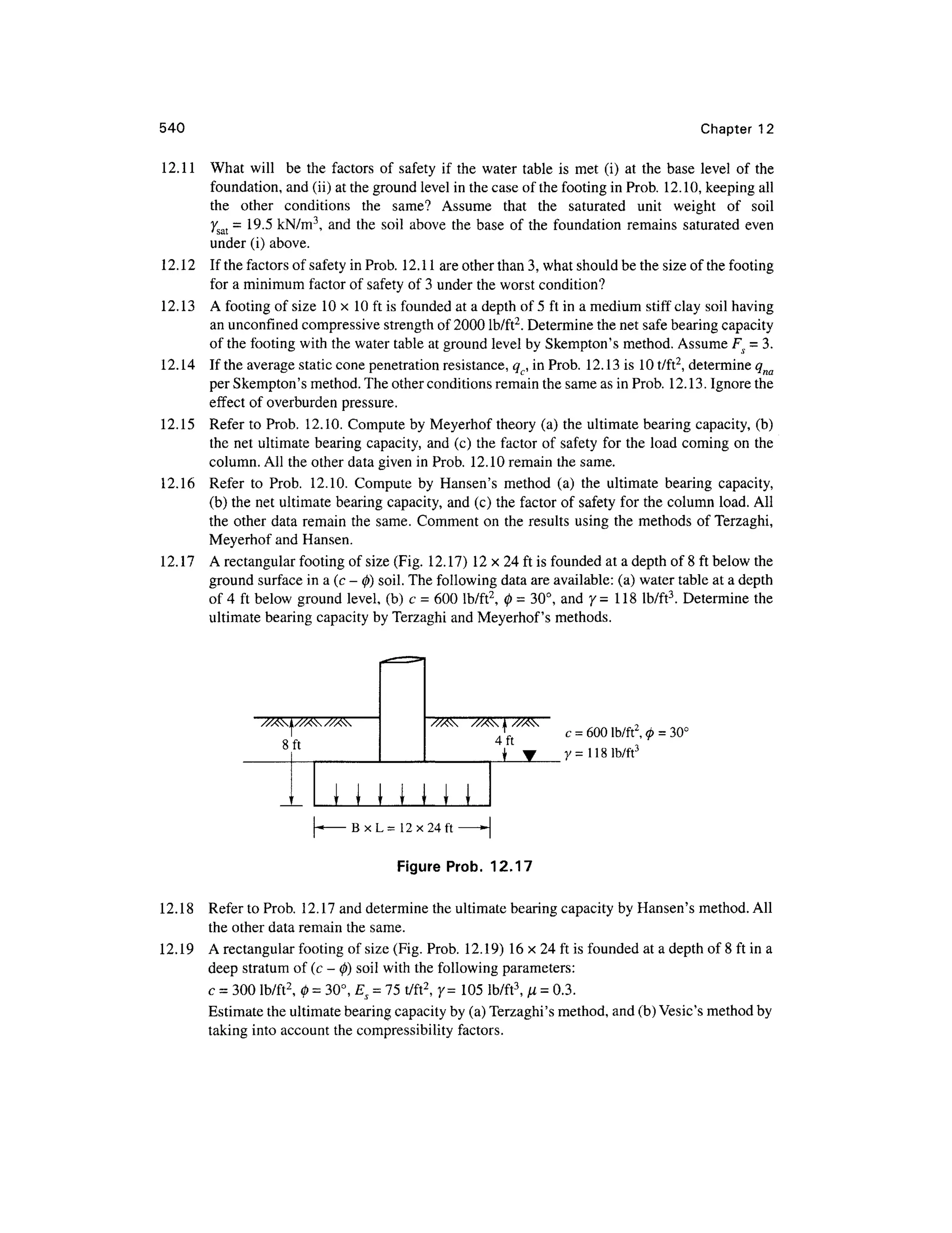
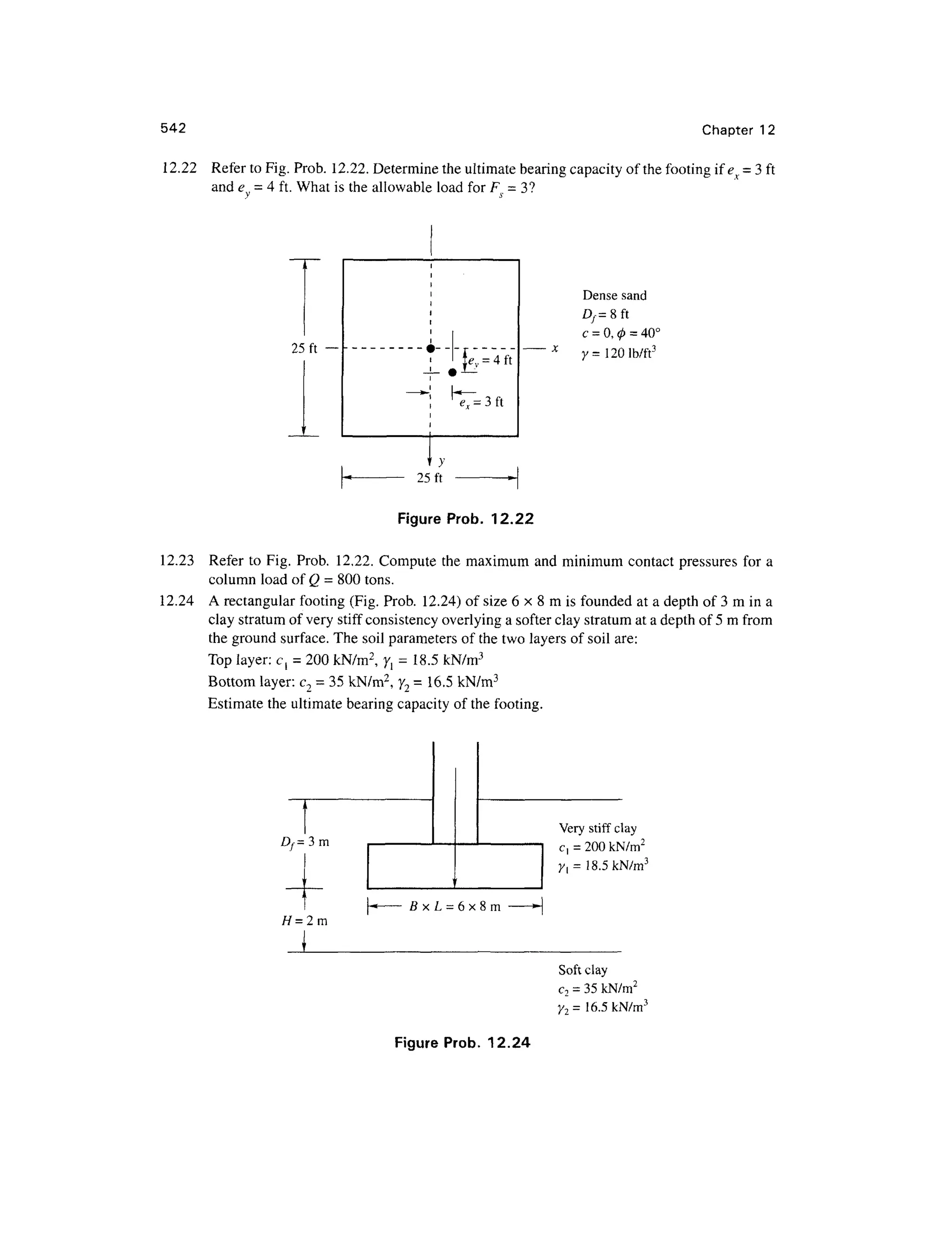
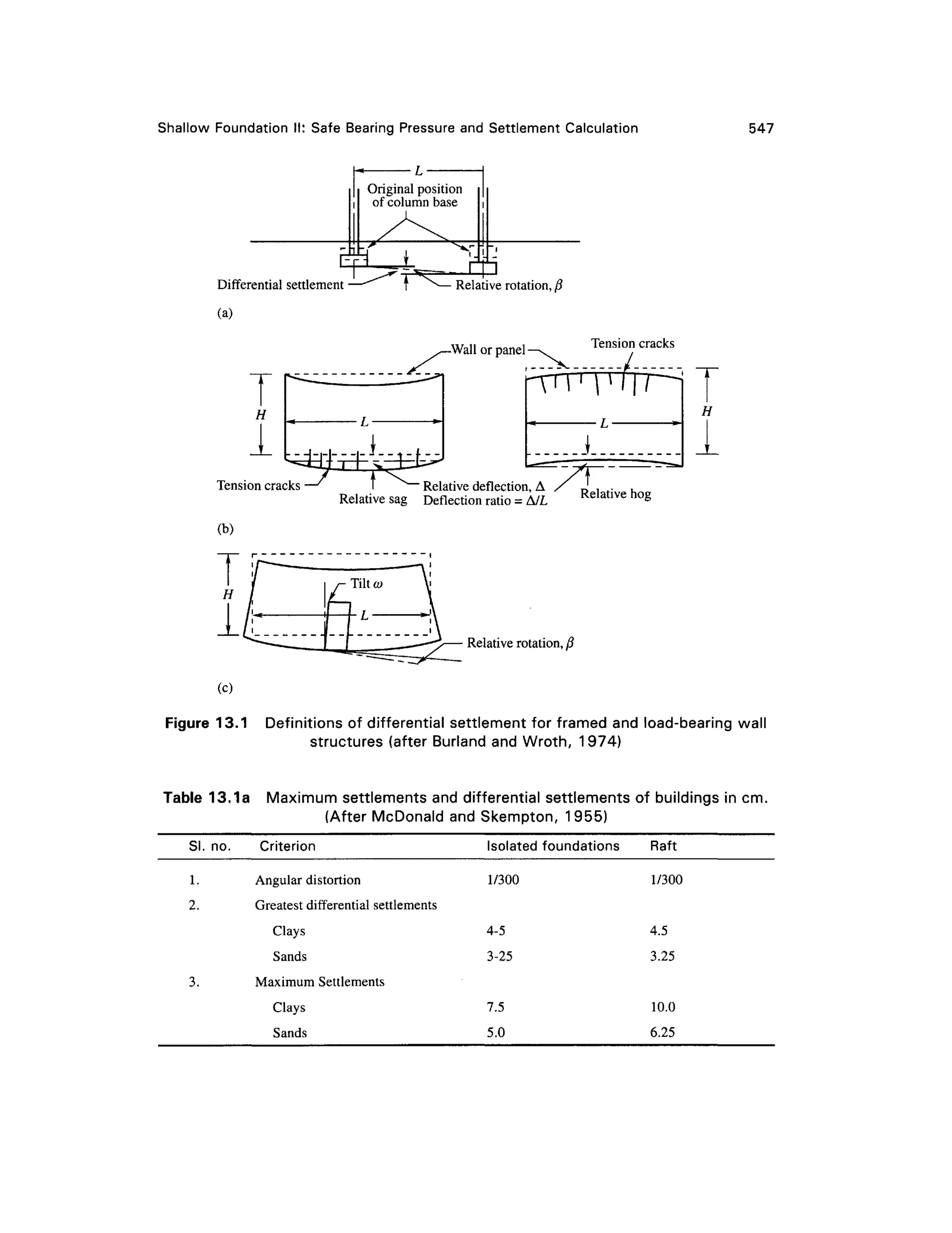
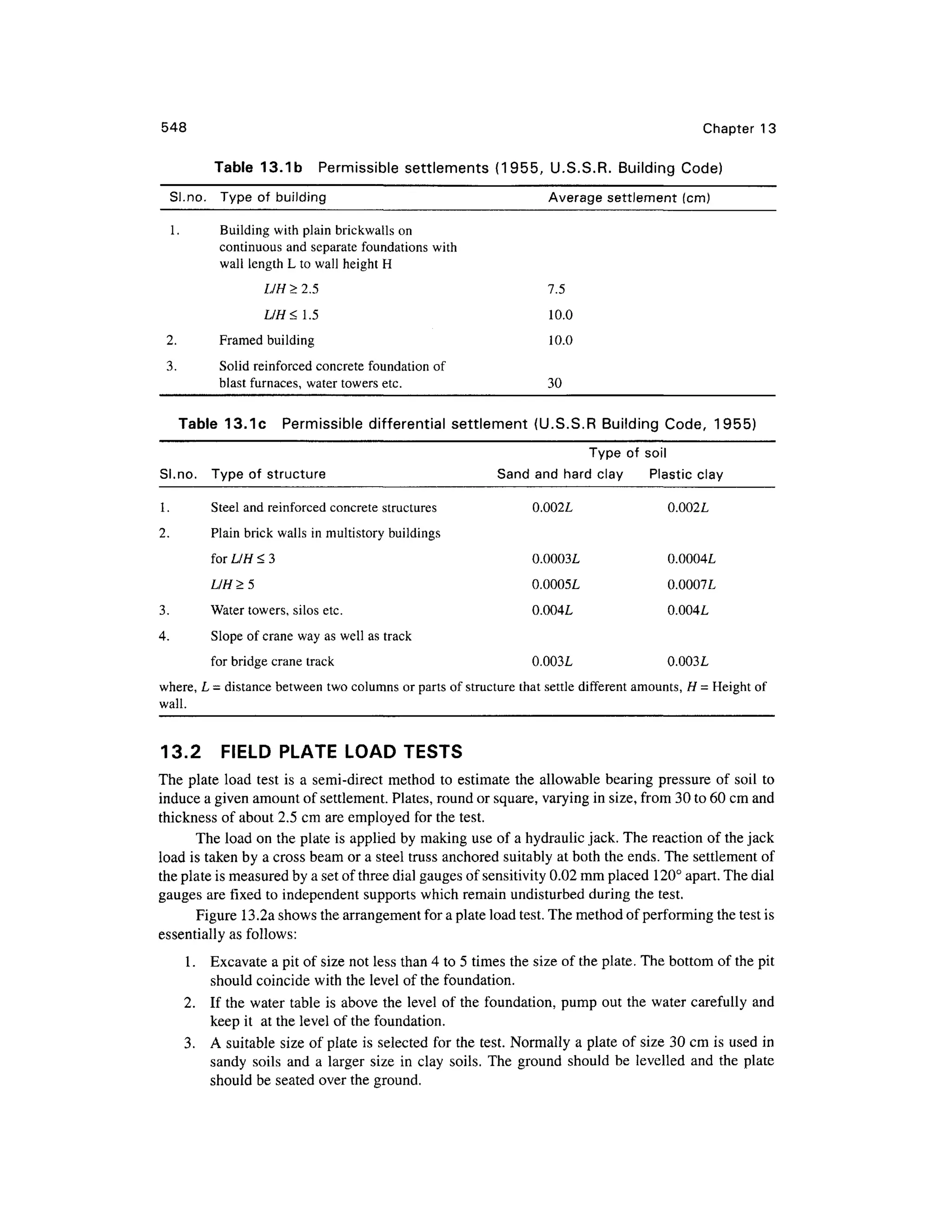
568. Shallow Foundatio n II : Safe Bearing Pressure and Settlement Calculatio n 549
rod -
|k
k^
ns —Channel
IL
Steel girders
g
5IC ^V- ^
""•^X ^-^ |
/ (
Anchors ^
1
r_
Extension ^
^
pipe ^~^ ^
rt
—I
13
L_
u
c=
3-1
^^_ Hydraulic
>^ jac k
p
Dial gau£
«h
4
;e
a
i
£55
T^^-^S; .^^Ita.
J]
£
^7 N
1 /
Y
S;
Test plate —/ |^ _ &p __^| > ^ Test pit
Section
^na
©
©
©
—
©
©
©
U1Ci
i
i
I
2 Girders
A
ii /
p
i . t i i i i
)
Test plate
ii
i
1
Support
©
©
©
n
1
©
©
©
4.
Top plan
Figure 13.2 a Plat e load test arrangemen t
A seating load of about 70 gm/cm2
is first applied and released after som e time. A higher
load is next placed on the plate and settlements are recorded by means of the dial gauges.
Observations on every load increment shall be taken until the rate of settlement is less than
0.25 mm per hour. Load increments shall be approximately one-fifth o f the estimated saf e
bearing capacity of the soil. The average of the settlements recorded by 2 or 3 dial gauges
shall be taken as the settlement of the plate for each of the load increments.
5. Th e test should continue until a total settlement of 2.5 cm or the settlement at which the soil
fails, whichever is earlier, is obtained. After the load is released, the elastic rebound of the
soil should be recorded.
From the test results, a load-settlement curve should be plotted as shown in Fig. 13.2b . The
allowable pressure on a prototype foundation for an assumed settlement may be found by making
use o f th e followin g equations suggeste d b y Terzagh i an d Pec k (1948 ) fo r squar e footing s in
granular soils.

569. 550 Chapter 1 3
Plate bearing pressure in kg/cm2
or T/m2
i q a = Ne
t allowable pressure
Figure 13.2 b Load-settlemen t curv e o f a plate-load tes t
B
Sf = S x —-
where 5 , =permissible settlemen t of foundation in mm,
S - settlemen t of plate in mm,
(IS.lb)
B = size of foundation in meters,
b = size of plate in meters.
For a plate 1 ft square, Eq. (13.la) may be expressed a s
iJ r — 0
f p (13.2)
in which S, and 5 ar e expressed i n inches and B in feet.
The permissibl e settlemen t 5 , for a prototyp e foundatio n shoul d b e known . Normall y a
settlement of 2.5 cm is recommended. I n Eqs (13.la) or (13.2) the values of 5, and b ar e known.
The unknown s ar e 5 an d B. The valu e o f S fo r an y assume d siz e B ma y be foun d fro m th e
equation. Usin g th e plat e loa d settlemen t curv e Fig . 13. 3 th e valu e o f th e bearin g pressur e
corresponding t o th e compute d valu e of 5 i s found . Thi s bearin g pressur e i s th e saf e bearin g
pressure fo r a given permissible settlemen t 5~ The principal shortcoming o f this approach i s the
unreliability of the extrapolation of Eqs (13. la) o r (13.2).
Since a load test is of short duration, consolidation settlements cannot be predicted. The test
gives the value of immediate settlement only. If the underlying soil is sandy in nature immediate
settlement may be taken as the total settlement. If the soil is a clayey type, the immediate settlement
is only a fraction of the total settlement . Loa d tests , therefore, do not have much significance in
clayey soils to determine allowable pressure on the basis of a settlement criterion.

570. Shallow Foundatio n II : Safe Bearing Pressure and Settlement Calculatio n 55 1
Pistp inaH T A •* Foundatio n o f
Flate load Loa d qn per unit area
test ^ca
/ buildin g
I
l
J
J
J
J
l
L
L
i
J
y/////////////////^^^^
Stiff clay
Soft cla y
Pressure bulbs
Figure 13.2c Plat e load test on non-homogeneous soi l
Plate load tests should be used with caution and the present practice is not to rely too much on
this test . I f the soi l i s no t homogeneous t o a great depth , plate loa d test s giv e ver y misleadin g
results.
Assume, as shown in Fig. 13.2c , two layers of soil. The top layer is stiff cla y whereas th e
bottom laye r i s sof t clay . The loa d tes t conducte d nea r th e surfac e of th e groun d measure s th e
characteristics of the stiff clay but does not indicate the nature of the soft clay soil which is below.
The actual foundation of a building however has a bulb of pressure which extends to a great depth
into the poor soi l whic h is highly compressible. Her e the soil tested b y the plate load tes t gives
results which are highly on the unsafe side .
A plate load test is not recommended in soils which are not homogeneous a t least to a depth
equal to l
/2 to 2 times the width of the prototype foundation.
Plate load tests should not be relied on to determine the ultimate bearing capacity of sandy
soils as the scale effect give s very misleading results. However, when the tests are carried on clay
soils, the ultimate bearing capacity as determined by the test may be taken as equal to that of the
foundation sinc e the bearing capacity of clay is essentially independent of the footing size.
Housel's (1929 ) Metho d o f Determinin g Saf e Bearin g Pressur e fro m
Settlement Consideratio n
The metho d suggeste d b y House l fo r determinin g th e saf e bearin g pressur e o n settlemen t
consideration is based on the following formula
O = A m + Pn C1 3 3)
^ p p ±~>.~> j
where Q = load applied on a given plate, A = contact area of plate, P = perimeter o f plate, m = a
constant corresponding t o the bearing pressure, n - anothe r constant corresponding t o perimeter
shear.
Objective
To determine the load (Xand the size of a foundation for a permissible settlemen t 5-..
Housel suggest s tw o plat e loa d test s wit h plate s o f differen t sizes , sa y B l x B^ an d
B2 x B2 for this purpose.

571. 552 Chapte r 1 3
Procedure
1 .Tw o plate load tests are to be conducted at the foundation level of the prototype as per the
procedure explained earlier.
2. Dra w the load-settlement curves for each of the plate load tests.
3. Selec t the permissible settlement S,. for the foundation.
4. Determin e the loads Q{ and Q2 from each of the curves for the given permissible settlemen t
sf
Now we may write the following equations
Q=mA
P+np
P (13.4a )
for plate load test 1 .
Q2=mAp2+nPp2 (13.4b )
for plate load test 2.
The unknown values of m and n can be found by solving the above Eqs. (13.4a) and (13. 5b).
The equation for a prototype foundation may be written as
Qf=mAf+nPf (13.5 )
where A, = area of the foundation, />,=perimeter of the foundation.
When A, and P,are known, the size of the foundation can be determined .
Example 13.
1
A plat e loa d tes t usin g a plat e o f siz e 3 0 x 3 0 cm wa s carrie d ou t a t th e leve l o f a prototyp e
foundation. Th e soi l a t the sit e wa s cohesionless wit h the wate r table a t grea t depth . The plat e
settled by 1 0 mm at a load intensity of 160 kN/m2
. Determine the settlement of a square footing of
size 2 x 2 m under the same load intensity.
Solution
The settlement of the foundation 5, may be determined from Eq. (13. la)
.
,
=3a24mm
Example 13.2
For Ex. 13. 1 estimate the load intensity if the permissible settlement of the prototype foundation is
limited to 40 mm.
Solution
In Ex. 13 . 1, a load intensity of 160 kN/m2
induces a settlement of 30.24 mm. If we assume that the
load-settlement is linear within a small range, we may write

572. Shallow Foundatio n II : Safe Bearing Pressure and Settlement Calculatio n 55 3
where, q{ = 160 kN/m2
, S^ = 30.24 mm, S^ = 40 mm. Substituting the known values
40
q2 = 160 x —— = 211.64 kN/m2
Example 13.3
Two plate load tests were conducted at the level of a prototype foundation in cohesionless soil close
to each other. The following data are given:
Size of plate
0.3 x 0.3 m
0.6 x 0.6 m
Load applied
30 kN
90 kN
Settlement recorded
25 mm
25 mm
If a footing is to carry a load of 1000 kN, determine the required size of the footing for the
same settlement of 25 mm.
Solution
Use Eq. (13.3). For the two plate load tests we may write:
PLTl: A pl = 0.3 x 0.3 =0.09m2
;P pl = 0.3 x4 = 1.2m; Q l = 30 kN
PLT2: A p2 = 0.6x0. 6 = 0.36m2
; P p2 = 0.6 x 4 = 2.4m; Q 2 = 90 kN
Now we have
30 = 0.09m + 1.2n
90 = 0.36m + 2.4n
On solving the equations we have
m = 166.67, and n = 12.
5
For prototype foundation, we may write
Qf = 166.67 A
f+ 12.5 Pf
Assume the size of the footing as B x B, we have
Af = B2
, P f = 4B, an d Q f = 1000 kN
Substituting we have
1000 =166.67fl2
+505
or B 2
+0.35-6 = 0
The solution gives B = 2.3 m.
The size of the footing = 2.3 x 2.3 m.

573. 554 Chapter 1 3
13.3 EFFEC T OF SIZE OF FOOTINGS O N SETTLEMEN T
Figure 13.3 a give s typica l load-settlemen t relationship s fo r footing s o f differen t width s o n th e
surface of a homogeneous san d deposit. It can be seen tha t the ultimate bearing capacitie s o f the
footings per unit area increase with the increase in the widths of the footings. However, for a given
settlement 5, such as 25 mm, the soil pressure is greater for a footing of intermediate width Bb than
for a large footing with BC. The pressures corresponding t o the three widths intermediate, large and
narrow, are indicated by points b, c and a respectively.
The same data is used to plot Fig. 13.3b which shows the pressure per unit area corresponding
to a given settlement 5j, as a function o f the width of the footing. The soil pressure for settlement
Sl increase s fo r increasin g widt h of th e footing , i f th e footing s ar e relativel y small , reache s a
maximum at an intermediate width, and then decreases graduall y with increasing width.
Although the relation shown in Fig. 13.3 b is generally vali d for the behavior of footings on
sand, it is influenced by several factors including the relative density of sand, the depth at which the
foundation i s established, an d the position of the water table. Furthermore, th e shape of the curve
suggests tha t for narro w footing s small variation s in the actual pressure, Fig . 13.3a , may lead t o
large variation in settlement and in some instances to settlements so large that the movement would
be considered a bearing capacity failure. On the other hand, a small change in pressure o n a wide
footing has little influence on settlements as small as S{ , and besides, the value of ql correspondin g
to Sj is far below that which produces a bearing capacity failure of the wide footing.
For al l practica l purposes , th e actua l curv e give n i n Fig . 13.3 b ca n b e replace d b y a n
equivalent curv e omn wher e o m i s the inclined part an d mn the horizonta l part . Th e horizonta l
portion of the curve indicates that the soil pressure corresponding t o a settlement S{ i s independent
of the size of the footing. The inclined portion om indicates the pressure increasin g with width for
the same given settlement S{ up to the point m on the curve which is the limit for a bearing capacity
Soil pressure, q
Given settlement, S
Narrow footin g
(a)
(b)
Width of footing, B
Figure 13. 3 Load-settlemen t curve s for footing s of differen t sizes
(Peck e t al., 1974 )

574. Shallow Foundatio n II : Safe Bearing Pressur e and Settlement Calculatio n 55 5
failure. Thi s mean s tha t the footing s up t o size Bl i n Fig. 13. 3b should be checked fo r bearin g
capacity failure also while selecting a safe bearing pressure by settlement consideration.
The position of the broken lines omn differs for different san d densities or in other words for
different SP T N values . The soi l pressur e tha t produce s a given settlemen t Sl o n loos e san d is
obviously smaller than the soil pressure that produces the same settlement on a dense sand. Since
N- value increases wit h density of sand, qs therefore increases with an increase in the value of N.
13.4 DESIG N CHARTS FROM SPT VALUES FOR FOOTINGS ON SAND
The methods suggested by Terzaghi et al., (1996) for estimating settlements an d bearing pressures
of footings founded on sand from SP T values ar e based on the findings of Burland and Burbidge
(1985). The SPT values used are corrected t o a standard energy ratio. The usual symbol Ncor is used
in all the cases as the corrected value .
Formulas fo r Settlemen t Calculation s
The following formulas were developed for computing settlements fo r square footings.
For normally consolidated soil s and gravels
cor
For preconsolidated san d and gravels
(13.6)
for q s>pc S c
= B°."-(qs-0.67pc) (13 .7a)
cor
—!± (I3.7b )
NIA
cor
If the footing is established at a depth below the ground surface, the removal of the soil above
the base leve l make s th e san d below th e base preconsolidate d b y excavation. Recompression i s
assumed for bearing pressures u p to preconstruction effective vertica l stress q'o at the base of the
foundation. Thus, for sands normally consolidated with respect to the original ground surface and
for values of qs greater than q'o, we have,
for q s>q'0 S c = B0
'75
-—(qs-Q.61q'0) (1 3 8a)
™ cor
for q s<q'0 S £ = jfi°-75
—— qs (13.8b )
where
Sc = settlemen t o f footing , i n mm , a t th e en d o f constructio n an d applicatio n o f
permanent live load
B - widt h of footing in m
qs = gros s bearin g pressur e o f footin g = QIA, i n kN/m 2
base d o n settlemen t
consideration
Q = tota l load on the foundation in kN
A= are a of foundation in m2
p= preconsolidatio n pressure in kN/m2

575. 556 Chapter 1 3
0.1 1 1 0
Breadth, B(m) — log scale
Figure 13. 4 Thicknes s o f granula r soil beneat h foundatio n contributin g t o
settlement, interpreted from settlement profile s (afte r Burlan d an d Burbidge 1985 )
q - effectiv e vertica l pressure at base level
N= averag e corrected N valu e within the depth of influence Z; below th e base th e of
footing
The depth of influence Z; is obtained from
Z^B0
-15
(13.9 )
Figure 13.4 give s th e variation o f the depth o f influence wit h depth base d on Eq. (13.9 )
(after Burlan d and Burbidge, 1985) .
The settlement of a rectangular footing of size B x L may be obtained from
2
(13.10)
L 1.25(1/8)
S(L/B>l) = S — = 1 -
c
B L I 5 + 0.25
when the ratio LIB is very high for a strip footing, we may write
Sc (strip)
Sr (square)
= 1.56 (13.11)
It may be noted here that the ground water table at the sit e may lie above or within the depth
of influenc e Z r Burlan d an d Burbidg e (1985 ) recommen d n o correctio n fo r th e settlemen t
calculation even if the water table lies within the depth of influence Z;. On the other hand, if for any
reason, the water table were to rise into or above the zone of influence Z7 after the penetration tests
were conducted, the actual settlement could be as much as twice the value predicted without taking
the water table into account.

576. Shallow Foundatio n II : Safe Bearing Pressur e and Settlement Calculatio n 557
Chart fo r Estimatin g Allowable Soi l Pressur e
Fig. 13. 5 give s a chart for estimating allowable bearing pressure qs (on settlement consideration)
corresponding to a settlement of 1 6 mm for different value s ofTV (corrected). From Eq. (13.6), an
expression for q ma y be written as (for normally consolidated sand)
NIA yyl.4
1.7fl°-75
where Q —
1.75 0.75
(13.12a)
(13,12b)
For sand having a preconsolidation pressure pc, Eq. (13.7) may be written as
for q s>pc q s
= 16Q+Q.61pc (13.13a )
for q s<pc q s= 3x6Q (13.13b )
If the sand beneath the base of the footing is preconsolidated because excavation has removed
a vertical effective stres s q'o, Eq. (13.8) may be written as
for q s>q'o, q s =16Q+Q.61q'o
for q s<q'0, q s
(13.14a)
(13.14b)
1 2 3 4 5 6 7 8 9 1 0 2 0 3 0
Width of footing (m)
Figure 13.5 Char t for estimatin g allowable soil pressure for footin g on sand on the
basis of result s o f standard penetratio n test . (Terzaghi, et al., 1996 )

577. 558 Chapte r 1 3
The char t m Fig . 13. 5 give s th e relationships between B an d Q . The valu e of qs ma y b e
obtained from Q for any given width B. The Q to be used must conform to Eqs (13.12), (13.13)
and (13.14).
The chart is constructed for square footings of width B. For rectangular footings, the value of
qs shoul d b e reduce d i n accordance wit h Eq . (13.10) . The bearin g pressure s determine d by thi s
procedure correspon d t o a maximum settlement of 25 mm at the end of construction.
It may be noted here that the design chart (Fig. 13.5b ) has been developed by taking the SPT
values corrected fo r 60 percent of standard energy ratio.
Example 13. 4
A square footing of size 4 x 4 m is founded at a depth of 2 m below the ground surface in loose to
medium dens e sand . The correcte d standar d penetration test valu e Ncor = 11 . Comput e th e safe
bearing pressur e qs b y usin g th e char t i n Fig . 13.5 . Th e wate r tabl e i s a t th e bas e leve l o f th e
foundation.
Solution
From Fig. 13. 5 Q = 5 for B = 4 m and Ncor = 11 .
From Eq . (13.12a)
q = 160 = 16x5 = 80 kN/m2
Example 13. 5
Refer to Example 13.4 . If the soil at the site is dense sand with Ncor = 30, estimate qs for B = 4 m.
Solution
From Fig. 13. 5 Q = 2 4 fo r B = 4m an d N= 30 .
^ *~- cor
FromEq. (13.12a)
<7s = 16Q = 16 x24 = 384 kN/m2
13.5 EMPIRICA L EQUATION S BASE D O N SP T VALUES FOR
FOOTINGS O N COHESIONLES S SOIL S
Footings o n granular soils are sometimes proportioned usin g empirical relationships. Teng (1969)
proposed an equation fo r a settlement of 25 mm based on the curves developed b y Terzaghi an d
Peck (1948). The modified form of the equation is
(13.15a)
where q - ne t allowable bearing pressure for a settlement of 25 mm in kN/m2
,
Ncor = corrected standar d penetration value
R= water table correction factor (Refer Section 12.7 )
WZ
Fd = depth factor = d + Df I B) < 2.0
B = width of footing in meters,
D,= depth of foundation in meters.

578. Shallow Foundatio n II : Safe Bearing Pressur e and Settlement Calculatio n 55 9
Meyerhof (1956 ) proposed th e following equations which are slightly different fro m that of
Teng
qs=2NcorRw2Fd fo r 5<1.2 m (13.15b )
Rw2FdforB>L2m (13.15c )
where Fd = (l+ 0.33 Df/B) < 1.33.
Experimental result s indicat e that the equations presented b y Teng an d Meyerhof ar e too
conservative. Bowles ( 1996) proposes an approximate increase of 50 percent over that of Meyerhof
which can also be applied to Teng's equations. Modified equations of Teng and Meyerhof are ,
Teng's equatio n (modified),
^=53(Afc o r -3) — ±^
- R w2Fd (13.16a )
Meyerhof 's equation (modified )
qs = 20NcorRw2FdforB<L2 m (13.16b )
s c o r R w2FdforB>l2m (13 .16c)
If the tolerable settlemen t is greater than 25 mm, the safe bearing pressure computed by the
above equations can be increased linearl y as,
where q's = net safe bearing pressure for a settlement S'mm, qs = net safe bearing pressure for a
settlement of 25 mm.
13.6 SAF E BEARIN G PRESSUR E FRO M EMPIRICA L EQUATIONS
BASED O N CP T VALUE S FO R FOOTINGS O N COHESIONLES S SOI L
The static cone penetration test in which a standard cone of 10 cm2
sectional area is pushed into the
soil without the necessity of boring provides a much more accurate and detailed variation in the soil
as discussed i n Chapter 9. Meyerhof (1956 ) suggeste d a set of empirical equation s based o n the
Terzaghi and Peck curves (1948). As these equations were also found to be conservative, modified
forms with an increase of 50 percent over the original values are given below.
qs = 3.6qcRw2 kPa fo r B < 1.2 m(13.17a )
( n 2
qs=2.lqc 1 + -
R w2kPa fo r 5>1.2 m (13.17b )
V DJ
An approximate formula for all widths
qs=2.7qcRw2kPa (13.17c )
where qc is the cone point resistance in kg/cm2
and qs in kPa.
The above equations have been developed for a settlement of 25 mm.

579. 560 Chapte r 1 3
Meyerhof (1956 ) develope d hi s equations based o n the relationship qc = 4Ncor kg/cm 2
for
penetration resistance i n sand where Ncor i s the corrected SP T value.
Example 13.6
Refer to Example 13.4 and compute qs by modified (a) Teng's method, and (b) Meyerhof 's method.
Solution
(a) Teng's equation (modified) —Eq. (13.16a)
i f D '
where R w2 = -
^1 +
- j =0.5 since Dw2 = 0
F, = +—£- = 1 + -= 1.5< 2
,
d
B 4
By substituting
qs -53(11 -3)1—1 x 0.5 x1.5 -92 kN/m2
(b) Meyerhof 's equation (modified ) —Eq
. (13.16c)
where R ,= 0.5, F , = l + 0.33x—f
- = l + 0.33x- = 1. 1 65 <1.33
w2 d B 4
By substituting
2
<?y = 12.5x11— x0.5x!.165-93kN/m 2
Note: Both the methods give the same result.
Example 13.7
A footing of size 3 x 3 m is to be constructed at a site at a depth of 1 .5 m below the ground surface.
The wate r tabl e i s at th e base o f the foundation. The averag e stati c con e penetratio n resistanc e
obtained a t the sit e is 20 kg/cm2
. The soi l is cohesive. Determin e th e safe bearing pressur e for a
settlement of 40 mm.
Solution
UseEq. (13.17b )

580. Shallow Foundatio n II : Safe Bearin g Pressur e and Settlement Calculatio n 56 1
B
where qc = 20 kg/cm2
, B = 3m,Rw2 = 0.5.
This equation is for 25 mm settlement. By substituting, we have
qs = 2.1 x201 1 + -I x 0.5 =37.3 kN/m2
For 40 mm settlement, the value of q i s
40
q = 37. 3 — = 6 0 kN/m2
*s
2 5
13.7 FOUNDATIO N SETTLEMEN T
Components of Total Settlement
The total settlement of a foundation comprises thre e parts as follows
S = Se+Sc+Ss (13.18 )
where S = tota l settlement
S
= elasti c or immediate settlement
Sc
= consolidatio n settlement
Ss
= secondar y settlemen t
Immediate settlement , Se, is tha t part of the total settlement , 5 1
, which i s suppose d t o tak e
place during the application of loading. The consolidation settlement is that part which is due to the
expulsion o f pore water fro m th e voids an d is time-dependent settlement . Secondar y settlemen t
normally start s wit h th e completio n o f th e consolidation . I t means , durin g th e stag e o f thi s
settlement, the pore water pressure is zero and the settlement is only due to the distortion of the soil
skeleton.
Footings founde d i n cohesionles s soil s reac h almos t th e fina l settlement , 5 , durin g th e
construction stag e itsel f du e t o the high permeability of soil. The wate r i n the voids i s expelle d
simultaneously wit h th e applicatio n o f loa d an d a s suc h th e immediat e an d consolidatio n
settlements in such soils are rolled into one.
In cohesive soils under saturated conditions, there is no change i n the water content during
the stage of immediate settlement . The soil mass is deformed without any change in volume soon
after th e applicatio n o f th e load . Thi s i s du e t o th e lo w permeabilit y o f th e soil . Wit h th e
advancement of time there will be gradual expulsion of water under the imposed excess load. The
time required for the complete expulsion of water and to reach zero water pressure may be several
years depending upon the permeability of the soil. Consolidation settlement may take many years
to reach its final stage . Secondary settlement is supposed to take place after th e completion of the
consolidation settlement, though in some of the organic soils there will be overlapping of the two
settlements to a certain extent.
Immediate settlements of cohesive soils and the total settlement of cohesionless soil s may be
estimated fro m elasti c theory . Th e stresse s an d displacement s depen d o n th e stress-strai n
characteristics o f the underlying soil. A realistic analysis is difficult becaus e these characteristic s
are nonlinear. Results from the theory of elasticity are generally used in practice, it being assumed
that the soi l i s homogeneous an d isotropic an d there i s a linear relationship between stres s and

581. 562 Chapter 1 3
Overburden pressure, p 0
Combined p0 an d Ap
D5= 1.5to2 B
0.1 to 0.2
Figure 13. 6 Overburde n pressur e and vertical stres s distribution
strain. A linea r stress-strai n relationshi p is approximatel y tru e whe n th e stres s level s ar e lo w
relative to the failure values. The use of elastic theory clearly involves considerable simplification
of the real soil.
Some o f th e result s from elasti c theor y require knowledge o f Young's modulu s (Es), her e
called the compression o r deformation modulus, Ed, and Poisson's ratio, jU, for the soil .
Seat o f Settlemen t
Footings founde d a t a dept h D, below th e surfac e settl e unde r th e impose d load s du e t o th e
compressibility characteristic s o f th e subsoil . The dept h throug h whic h th e soi l i s compresse d
depends upo n the distribution of effective vertica l pressure p'Q of the overburden and the vertical
induced stress A/? resulting from th e net foundation pressure qn as shown in Fig. 13.6 .
In the case of deep compressible soils, the lowest level considered in the settlement analysis
is the point where the vertical induced stress A/? is of the order of 0.1 to 0.2qn, where qn is the net
pressure on the foundation from the superstructure. This depth works out to about 1.5 to 2 times the
width o f th e footing . Th e soi l lyin g withi n thi s dept h get s compresse d du e t o th e impose d
foundation pressure and causes more than 80 percent of the settlement of the structure. This depth
DS is called as the zone of significant stress. If the thickness of this zone is more than 3 m, the steps
to be followed in the settlement analysis are
1. Divid e the zone of significant stress into layers of thickness not exceeding 3 m,
2. Determin e the effective overburde n pressure p'o at the center of each layer,
3. Determin e the increase in vertical stress Ap due to foundation pressure q a t the center of
each layer along the center line of the footing by the theory of elasticity,
4. Determin e th e averag e modulu s of elasticit y and othe r soi l parameter s fo r eac h o f th e
layers.
13.8 EVALUATIO N O F MODULUS O F ELASTICITY
The most difficult part of a settlement analysis is the evaluation of the modulus of elasticity Es, that
would confor m t o th e soi l conditio n i n th e field . Ther e ar e tw o method s b y whic h E s ca n b e
evaluated. They are

582. Shallow Foundatio n II : Safe Bearing Pressur e and Settlement Calculatio n 56 3
1. Laborator y method,
2. Fiel d method .
Laboratory Metho d
For settlement analysis, the values of Es at different depths below the foundation base are required.
One wa y o f determinin g Es i s t o conduc t triaxia l test s o n representativ e undisturbe d samples
extracted from the depths required. For cohesive soils, undrained triaxial tests and for cohesionless
soils draine d triaxia l tests ar e required. Sinc e i t is practically impossible t o obtai n undisturbed
sample o f cohesionless soils , the laboratory method of obtaining Es ca n be ruled out. Even with
regards to cohesive soils, there will be disturbance to the sample at different stage s of handling it,
and a s suc h th e value s of E S obtaine d fro m undraine d triaxial tests d o no t represen t th e actua l
conditions and normally give very low values. A suggestion is to determine Es over the range of
stress relevant to the particular problem. Poulos et al., (1980) suggest that the undisturbed triaxial
specimen be given a preliminary preconsolidation under KQ conditions with an axial stress equal to
the effectiv e overburde n pressur e a t the samplin g depth. This procedur e attempt s t o retur n th e
specimen to its original state of effective stress in the ground, assuming that the horizontal effective
stress in the ground was the same as that produced by the laboratory KQ condition. Simons and Som
(1970) have shown that triaxial tests on London clay in which specimens were brought back to their
original i n situ stresse s gav e elastic modul i which were muc h higher than those obtained fro m
conventional undrained triaxial tests. This has been confirmed by Marsland (1971) who carried out
865 mm diameter plate loading tests in 900 mm diameter bored holes i n London clay. Marsland
found tha t the average modul i determined fro m th e loading tests wer e between 1. 8 to 4.8 time s
those obtained from undrained triaxial tests. A suggestion to obtain the more realistic value for Es
is,
1. Undisturbe d samples obtained from the field must be reconsolidated under a stress system
equal to that in the field (^-condition),
2. Sample s must be reconsolidated isotropicall y to a stress equal to 1/ 2 to 2/3 of the in situ
vertical stress.
It ma y b e note d her e tha t reconsolidatio n o f disturbe d sensitiv e clay s woul d lea d t o
significant change in the water content and hence a stiffer structure which would lead to a very high
E,-
Because o f th e man y difficultie s face d i n selectin g a modulu s valu e fro m th e result s of
laboratory tests, it has been suggested that a correlation between the modulus of elasticity of soil
and the undrained shear strength may provide a basis for settlement calculation. The modulus E
may be expressed as
Es = Acu (13.19 )
where the value of A for inorganic stiff clay varies from about 500 to 1500 (Bjerrum , 1972 ) an d cu
is the undrained cohesion. It may generally be assumed that highly plastic clays give lower values
for A, and low plasticity give higher values for A. For organic or soft clays the value of A may vary
from 10 0 t o 500 . Th e undraine d cohesio n c u ca n be obtaine d fro m an y on e o f th e fiel d test s
mentioned below and also discussed in Chapter 9.
Field methods
Field method s ar e increasingl y used t o determine th e soil strengt h parameters. The y hav e been
found t o be mor e reliabl e tha n the ones obtaine d fro m laborator y tests . Th e fiel d test s tha t are
normally used for this purpose are
1. Plat e load tests (PLT)

583. 564 Chapte r 1 3
Table 13. 2 Equation s fo r computin g Es by makin g us e of SP T and CP T values (i n
kPa)
Soil SP T CP T
Sand (normally consolidated) 50 0 (Ncor +15 ) 2 to 4 qc
(35000 to 50000) log Ncor (+D r
2
)qc
(U.S.S.R Practice)
Sand (saturated) 25 0 (N +15 )
Sand (overconsolidated) - 6 to 30 qc
Gravelly sand and gravel 120 0 (N + 6)
Clayey sand 32 0 (Ncor +15 ) 3 to 6 qc
Silty sand 30 0 (Ncor + 6) 1 to 2 qc
Soft cla y - 3 to 8 qc
2. Standar d penetration test (SPT )
3. Stati c cone penetration test (CPT )
4. Pressuremete r tes t (PMT )
5. Fla t dilatometer test (DMT )
Plate loa d tests , i f conducted a t levels at which Es i s required, giv e quite reliable value s as
compared to laboratory tests. Since these tests are too expensive to carry out, they are rarely use d
except i n major projects.
Many investigators have obtained correlations betwee n E g an d field test s suc h as SPT, CP T
and PMT. The correlations between ES and SPT or CPT are applicable mostly to cohesionless soil s
and in some cases cohesive soils under undrained conditions. PMT can be used for cohesive soils to
determine both the immediate and consolidation settlements together .
Some of the correlations o f £y with N and qc are given in Table 13.2 . These correlations hav e
been collecte d from variou s sources.
13.9 METHOD S O F COMPUTING SETTLEMENTS
Many methods are available for computing elastic (immediate) and consolidation settlements. Only
those method s tha t are of practical interes t are discussed here. The'variou s methods discusse d i n
this chapter are the following:
Computation of Elasti c Settlement s
1. Elasti c settlemen t base d on the theory of elasticity
2. Janb u e t al., (1956) method of determining settlement under an undrained condition.
3. Schmertmann' s method of calculating settlement in granular soils by using CPT values.
Computation o f Consolidatio n Settlemen t
1. e-og p metho d by making use of oedometer tes t data.
2. Skempton-Bjerru m method.

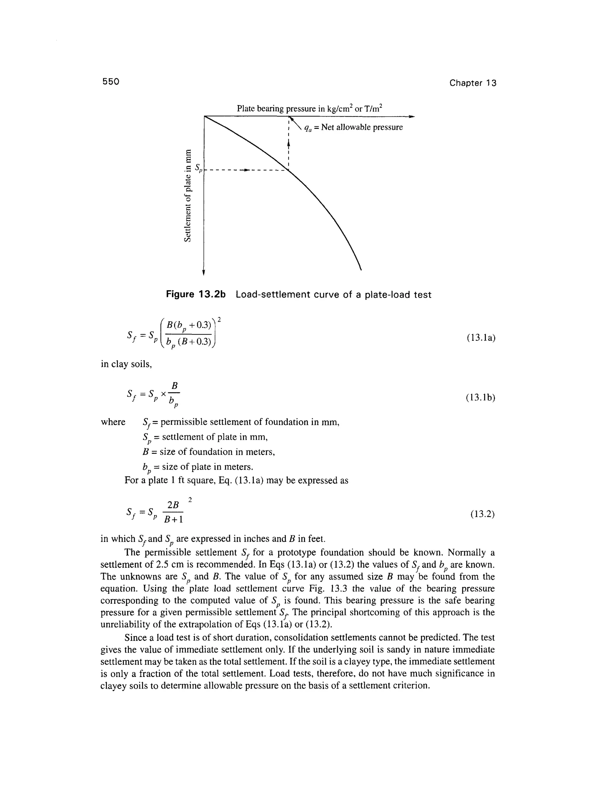
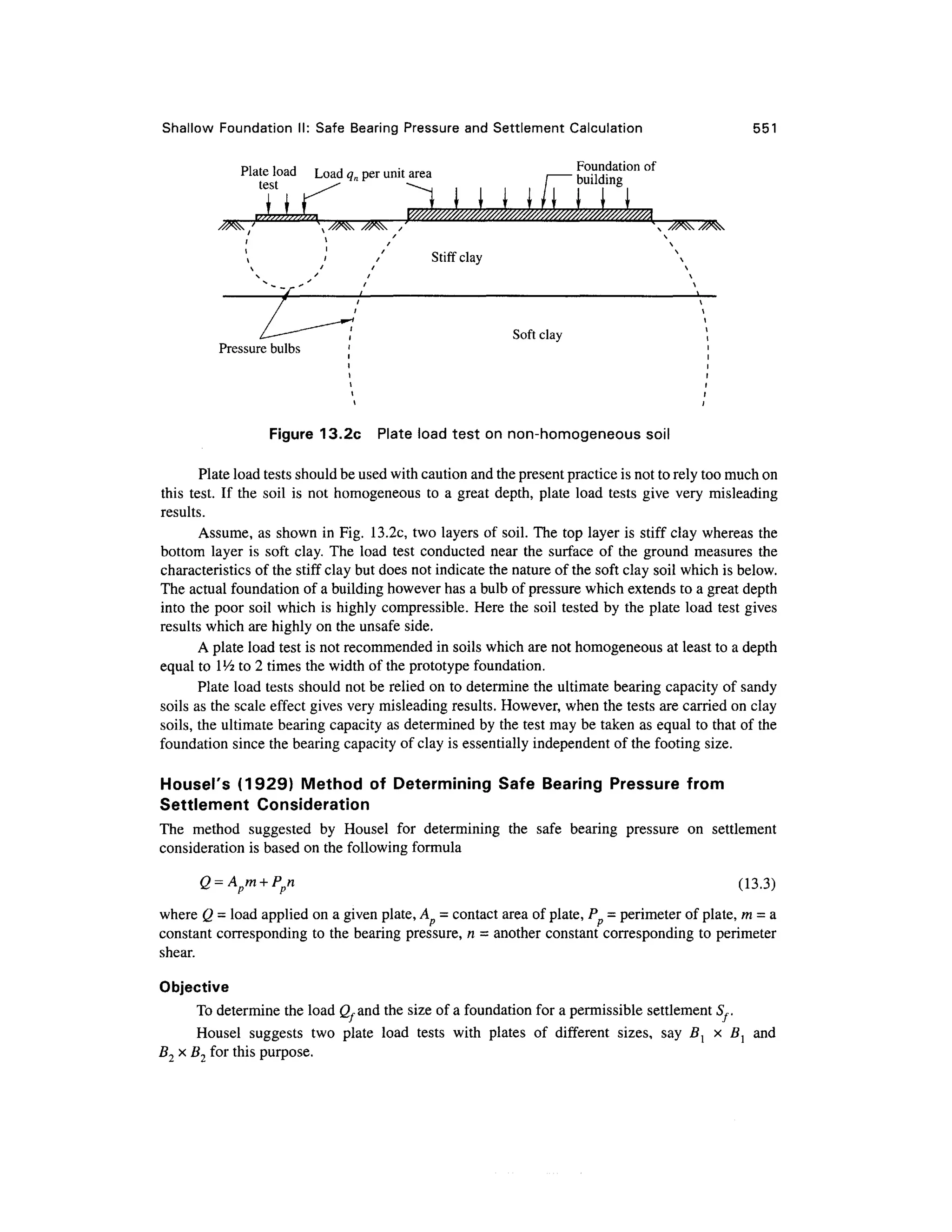
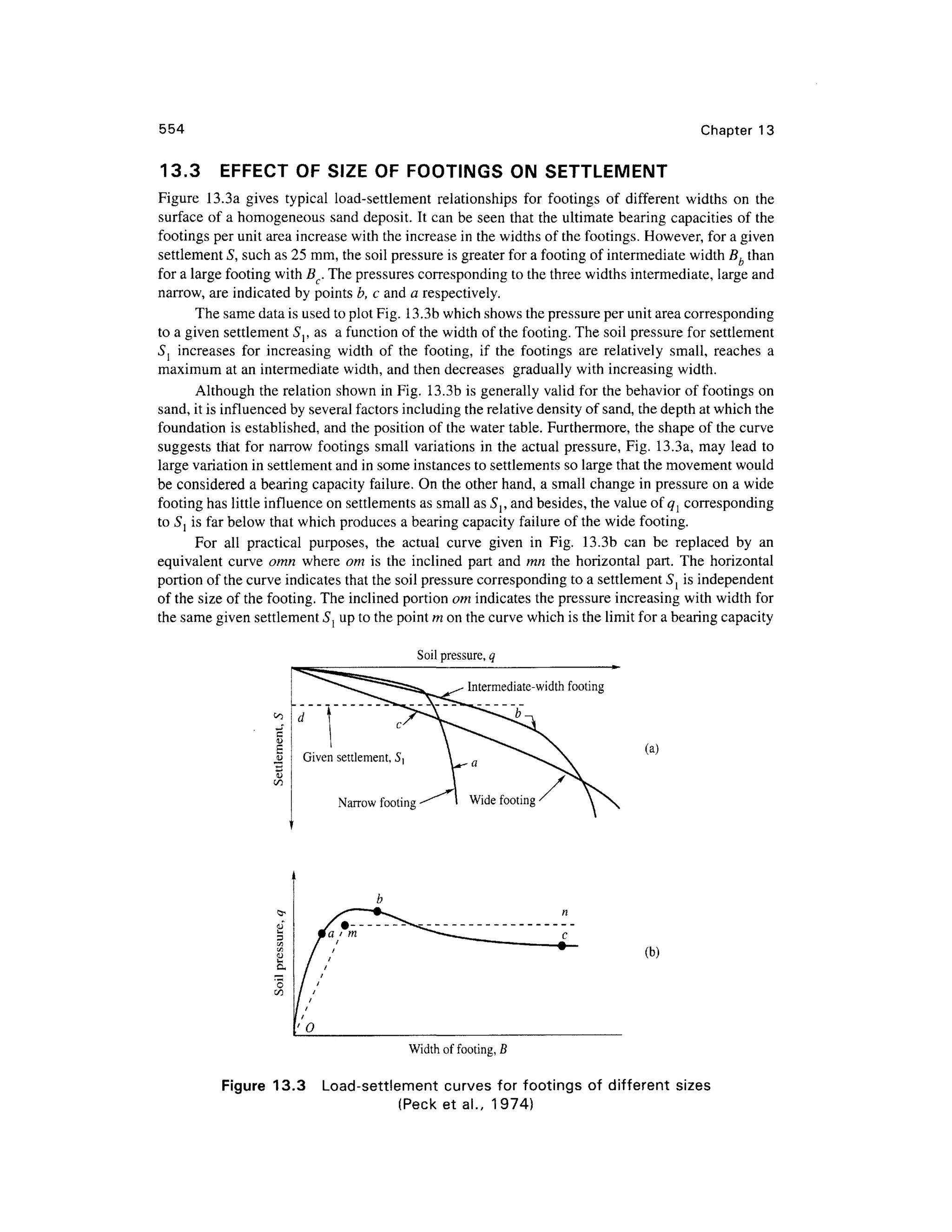
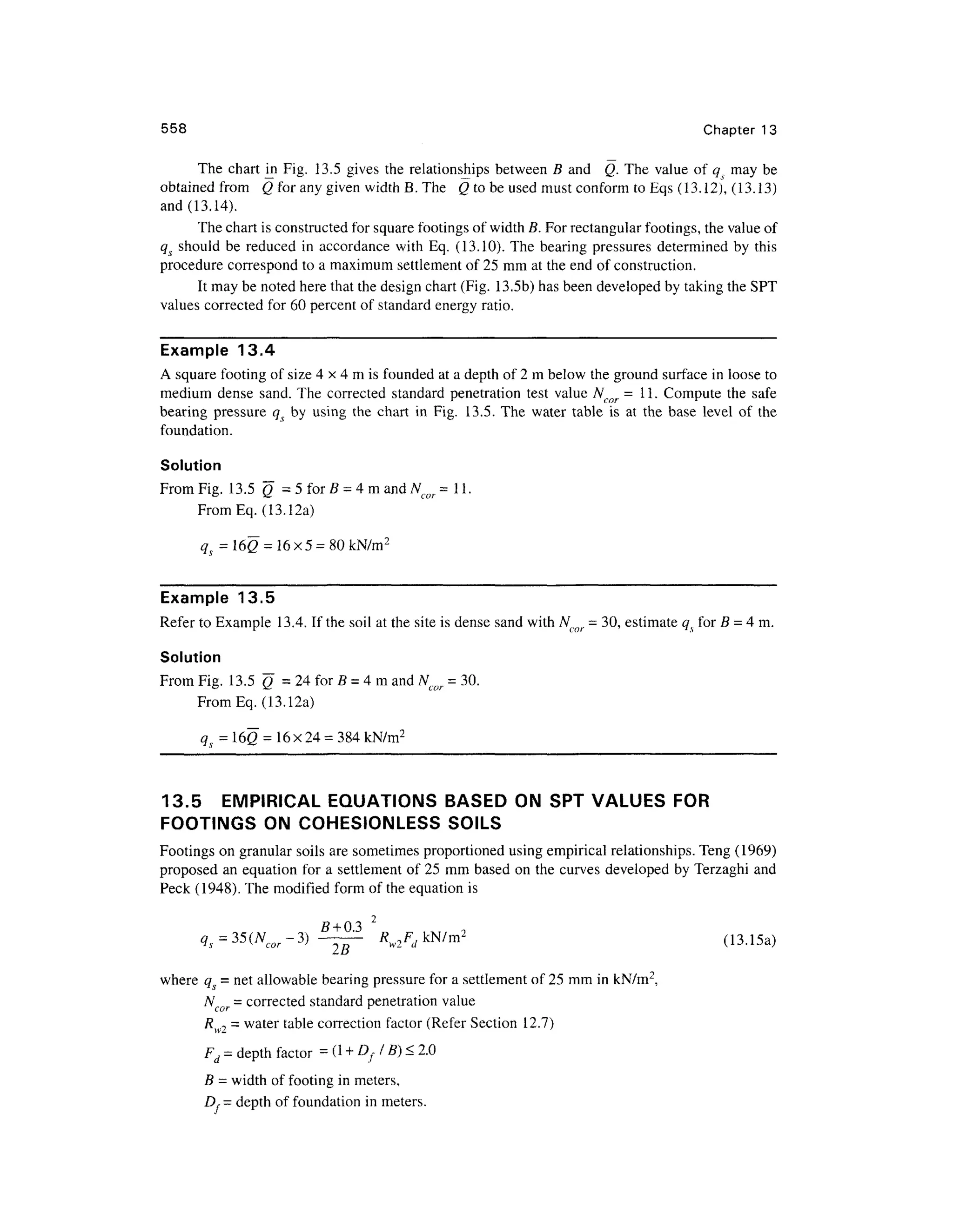
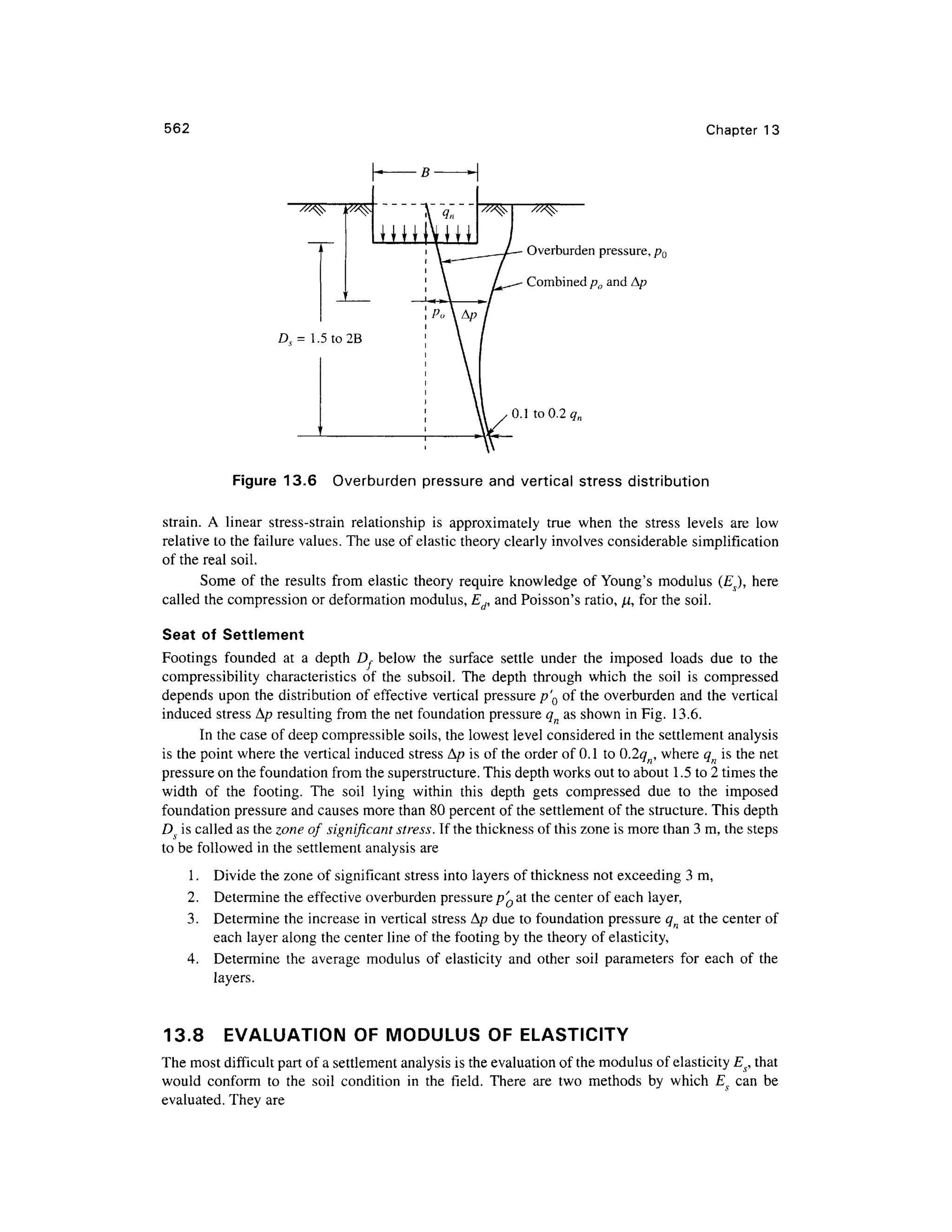
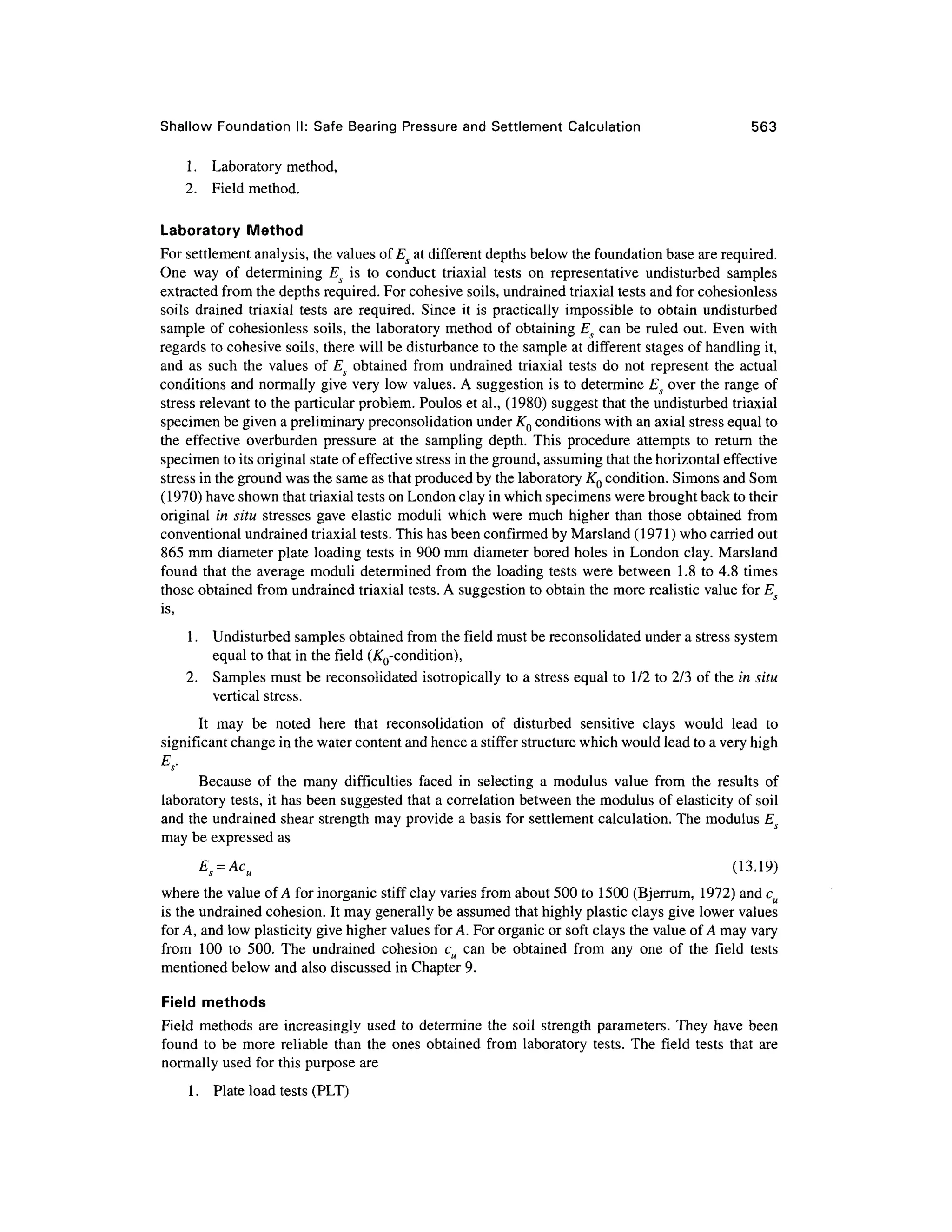
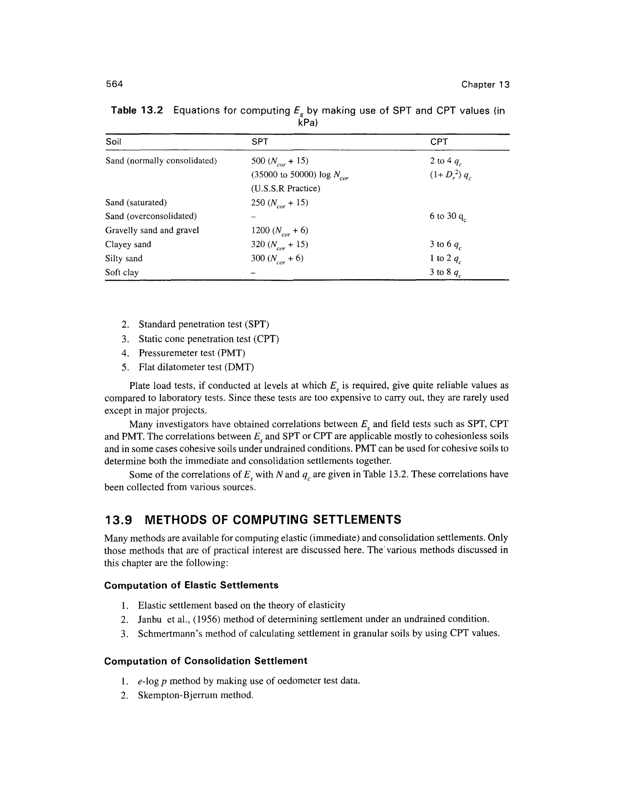
584. Shallow Foundatio n II: Safe Bearing Pressur e and Settlement Calculatio n 56 5
13.10 ELASTI C SETTLEMEN T BENEAT H TH E CORNE R OF A
UNIFORMLY LOADE D FLEXIBL E AREA BASE D O N TH E THEOR Y O F
ELASTICITY
The net elastic settlement equation for a flexible surface footing may be written as,
c P a->"2
),
S=B-— -
I
f (13.20a )
s
where S e= elasti c settlement
B = widt h of foundation,
Es = modulu s of elasticity of soil,
fj,= Poisson' s ratio ,
qn = ne t foundation pressure,
7, = influenc e factor.
In Eq . (13.20a) , fo r saturate d clays ,JL - 0.5 , and E s i s t o b e obtaine d unde r undrained
conditions as discussed earlier. For soils other than clays, the value of ^ has to be chosen suitably
and the corresponding valu e of Es has to be determined. Table 13.3 gives typical values for /i as
suggested by Bowles (1996) .
7, is a function o f the LIB ratio of the foundation, and the thickness H of the compressibl e
layer. Terzaghi has a given a method of calculating 7, from curves derived by Steinbrenner (1934) ,
for Poisson's ratio of 0.5, 7, = F1?
for Poisson's rati o of zero, 7,= F7 + F2.
where F{ an d F2 are factors which depend upon the ratios of H/B and LIB.
For intermediate values of //, the value of If can be computed by means of interpolation or by
the equation
(l-f,-2f,2
)F2
(13.20b)
The value s o f F j an d F 2 ar e give n i n Fig. 13.7a. Th e elasti c settlemen t a t an y poin t N
(Fig. 13.7b ) is given by
(I-//2
)
Se a t point N = -S-_ [/ ^ + If2B2 + 7/37?3 + 7/47?4] (1 3 20c)
Table 13. 3 Typica l rang e of value s for Poisson' s rati o (Bowles , 1996 )
Type o f soi l y.
Clay, saturated 0.4-0. 5
Clay, unsaturated 0.1-0. 3
Sandy clay 0.2-0. 3
Silt 0.3-0.3 5
Sand (dense ) 0.2-0. 4
Coarse (void ratio 0.4 to 0.7) 0.1 5
Fine grained (void ratio = 0.4 to 0.7) 0.2 5
Rock 0.1-0. 4

585. 566 Chapter 1 3
Values of F, _)andF2 ( _ _ _
0.1 0. 2 0. 3 0. 4 0. 5 0. 6 0. 7
Figure 13. 7 Settlemen t due to loa d on surface o f elasti c laye r (a ) F1 and F2 versu s
H/B (b) Method of estimating settlement (Afte r Steinbrenner , 1934 )
To obtain th e settlemen t a t the center o f the loade d area , the principle o f superpositio n i s
followed. In such a case N in Fig. 13.7 b will be at the center of the area when B{ = B4 = L2 = B3 and
B2 = L
r Then the settlement a t the center is equal to four times the settlement a t any one corner. The
curves in Fig. 13.7 a ar e based o n the assumption that the modulus of deformation is constant with
depth.
In the case of a rigid foundation, the immediate settlement at the center is approximately 0. 8
times tha t obtaine d fo r a flexible foundation a t the center . A correction facto r i s applie d t o th e
immediate settlemen t to allow for the depth of foundation by means of the depth factor d~ Fig. 13. 8
gives Fox's (1948) correctio n curv e for depth factor. The final elastic settlemen t i s
(13.21)
where,
"f=
s =
final elastic settlement
rigidity factor taken as equal to 0.8 for a highly rigid foundation
depth factor from Fig . 13. 8
settlement for a surface flexible footing
Bowles (1996) has given the influence factor for various shapes of rigid and flexible footings
as shown in Table 13.4 .

586. Shallow Foundatio n II : Safe Bearin g Pressur e and Settlement Calculatio n
Table 13. 4 Influenc e facto r lf (Bowles , 1988 )
567
Shape
Circle
Square
Rectangle
L/B= 1. 5
2.0
5.0
10.0
100.0
Flexible
0.85
0.95
1.20
1.20
1.31
1.83
2.25
2.96
lf (averag e values)
footing Rigi d footing
0.88
0.82
1.06
1.06
1.20
1.70
2.10
3.40
Corrected settlemen t for foundation of depth D ,
T~lr-ritli fnr^tn r —
Calculated settlement for foundation at surface
Q.50 0.6 0 0.7 0 0.8 0 0.9 0 1. 0
j
Df/^BL
•V
0.1
0.2
0.3
0.4
0.5
0.6
0.7
0.8
0.9
1 n
0.9
0.8
0.7
0.6
0.5
0.4
0.3
0.2
0.1
_ n
1-
9-
L
r
' D,
r
i
m
'//
7TT
y
/
/ /
^/
r /
1
1
!
!
'/
1
j
ll>
//
r
I
k
1
I
/
100
25-
/
I//
//
<
—»
<7/
'/<
/
/
'rf
4y
/^
*l
/
-9
- 1
Numbers denote ratio L/B
25
-100
Figure 13. 8 Correctio n curves for elasti c settlemen t o f flexibl e rectangula r
foundations a t depth (Fox , 1948)

587. 568 Chapter 1 3
13.11 JANBU , BJERRU M AN D KJAERNSLI' S METHOD OF
DETERMINING ELASTI C SETTLEMEN T UNDE R UNDRAINE D
CONDITIONS
Probably th e most usefu l char t is that given by Janbu et al., (1956) as modified by Christian and
Carrier (1978 ) fo r the case of a constant Es wit h respect to depth. The chart (Fig . 13.9 ) provide s
estimates o f th e averag e immediat e settlemen t o f uniforml y loaded, flexibl e strip , rectangular ,
square or circular footings on homogeneous isotropi c saturate d clay. The equation for computing
the settlement ma y be expressed a s
S = (13.22)
In Eq. (13.20), Poisson's ratio is assumed equal to 0.5. The factors fiQ and ^are related to the
DJB an d HIB ratio s of the foundation as shown in Fig. 13.9 . Values ofJL^ ar e given for various LIB
ratios. Rigidit y and depth factor s are required t o be applied to Eq. (13.22) as per Eq. (13.21). In
Fig. 13. 9 th e thicknes s o f compressibl e strat a i s take n a s equa l t o H belo w th e bas e o f th e
foundation where a hard stratum is met with.
Generally, rea l soi l profile s whic h ar e deposite d naturall y consis t o f layer s o f soil s o f
different propertie s underlai n ultimatel y b y a har d stratum . Withi n thes e layers , strengt h an d
moduli generally increas e with depth. The chart given in Fig. 13. 9 ma y be used for the case of ES
increasing wit h depth by replacing the multilayered system with one hypothetical layer on a rigid
D
1.0
0.9
Incompressible
10
Df/B
15 2 0
1000
Figure 13. 9 Factor s for calculatin g the averag e immediate settlement o f a loade d
area (afte r Christian an d Carrier, 1978 )

588. Shallow Foundatio n II : Safe Bearin g Pressur e and Settlement Calculatio n 56 9
base. The depth of this hypothetical layer is successively extended to incorporate each real layer,
the correspondin g value s o f E s bein g ascribe d i n eac h cas e an d settlement s calculated . B y
subtracting the effect o f the hypothetical layer above each real layer the separate compressio n of
each layer may be found and summed to give the overall total settlement.
13.12 SCHMERTMANN' S METHO D O F CALCULATIN G
SETTLEMENT I N GRANULA R SOILS BY USING CR T VALUE S
It is normally taken for granted that the distribution of vertical strain under the center of a footing
over uniform sand is qualitatively similar to the distribution of the increase in vertical stress. If true,
the greatest strain would occur immediately under the footing, which is the position of the greatest
stress increase. The detailed investigation s of Schmertmann (1970), Eggestad , (1963 ) an d others,
indicate that the greatest strain would occur at a depth equal to half the width for a square or circular
footing. The strain is assumed to increase from a minimum at the base to a maximum at B/2, then
decrease and reaches zero at a depth equal to 2B. For strip footings of L/B > 10, the maximum strain
is found to occur at a depth equal to the width and reaches zero at a depth equal to 4B. The modified
triangular vertical strain influence factor distribution diagram as proposed by Schmertmann (1978)
is show n in Fig. 13.10 . The are a o f this diagram i s related t o the settlement . The equatio n (fo
r
square as well as circular footings) is
IB l
-jj-te (13.23 )
^ s
where, S = tota l settlement ,
qn = ne t foundation base pressure = (q -q' Q),
q = tota l foundation pressure,
q'0 = effectiv e overburden pressure at foundation level,
Az= thicknes s of elemental layer,
lz = vertica l strain influence factor,
Cj= dept h correction factor,
C2 = cree p factor.
The equations for Cl and C2 are
c
i = 1
~0-5 -7 - (13.24 )
C2 = l + 0.21og10 (13>2 5)
where t is time in years for which period settlement is required.
Equation (13.25) is also applicable for LIB > 10 except that the summation is from 0 to 4B.
The modulus of elasticity to be used in Eq. (13.25) depends upon the type of foundation as
follows:
For a square footing,
Es = 2.5qc (13.26 )
For a strip footing, LIB > 10,
E=3.5fl (13.27 )

589. 570 Chapter 1 3
Rigid foundation vertical strain
influence factor I z
0 0. 1 0. 2 0. 3 0. 4 0. 5 0. 6
tfl
to
N>
Co
> 3 B
C*
4BL
L/B > 10
>Peak/= 0.5 +0.1.
D
/;
.
•>
IH
-1,,
m
B/2 for LIB = 1
B for LIB > 10
ill
HI
Depth to peak /,
Figure 13.10 Vertica l strain Influence factor diagrams (after Schmertmann e t al., 1978 )
Fig. 13.1 0 gives the vertical strai n influence factor /z distribution for both squar e and strip
foundations if the ratio LIB > 10. Values for rectangular foundations for LIB < 10 can be obtained by
interpolation. Th e depth s a t whic h th e maximu m / z occur s ma y b e calculate d a s follow s
(Fig 13.10) ,
(13.28)
where p' Q = effectiv e overburde n pressur e a t depth s B/ 2 an d B fo r squar e an d stri p
foundations respectively.
Further, / i s equal to 0.1 at the base and zero at depth 2B below the base for square footing;
whereas for a strip foundation it is 0.2 at the base and zero at depth 4B.
Values of E5 given in Eqs. (13.26) and (13.27) are suggested by Schmertmann (1978). Lunne
and Christoffersen (1985 ) proposed the use of the tangent modulus on the basis of a comprehensive
review of field and laboratory tests as follows:
For normally consolidated sands,
(13.29)
£5 = 4 4c for 9c < 10
Es = (2qc + 20)for0<q c<50
Es= 12 0 for qc > 50
For overconsolidated sands with an overconsolidation rati o greater than 2,
(13.30)
(13.31)
(13.32a)
Es = 250 for qc > 50 (13.32b )
where Es and qc are expressed i n MPa.
The cone resistance diagram is divided into layers of approximately constant values of qc and
the strain influence factor diagram is placed alongside this diagram beneath the foundation which is

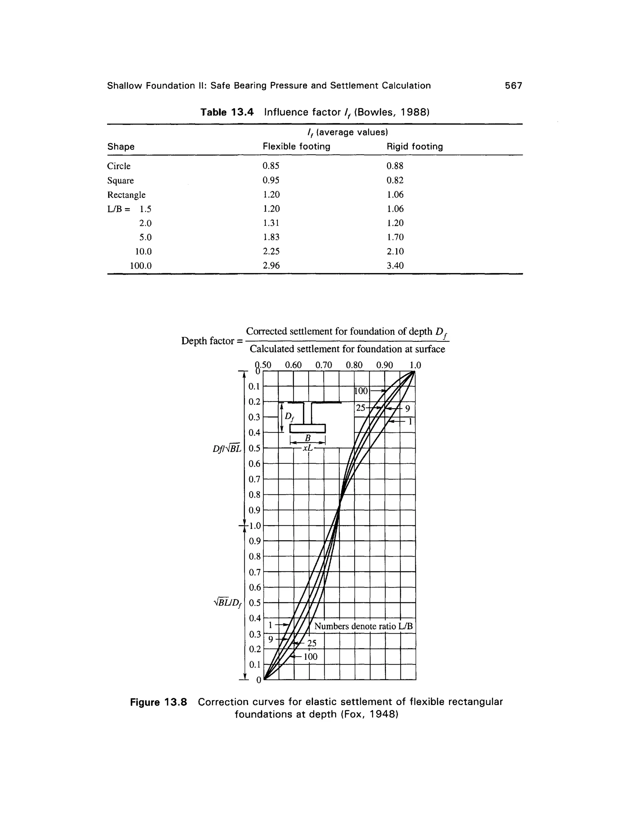
590. Shallow Foundatio n II: Safe Bearin g Pressur e an d Settlement Calculation 571
drawn to the same scale. The settlements of each layer resulting from the net contact pressure qn are
then calculated using the values of Es and /z appropriate to each layer. The sum of the settlements in
each laye r i s the n correcte d fo r th e dept h an d cree p factor s usin g Eqs. (13.24) an d (13.25 )
respectively.
Example 13.8
Estimate the immediate settlement of a concrete footing 1.5 x 1. 5 m in size founded at a depth of
1 m in silty soil whose modulus of elasticity is 90 kg/cm2
. The footing is expected to transmit a unit
pressure of 200 kN/m2
.
Solution
Use Eq. (13.20a)
Immediate settlement ,
s =
E
Assume n =0.35, /,
=0.82 for a rigid footing.
Given: q = 200 kN/m2
, B = 1.5 m, Es = 90 kg/cm2
« 9000 kN/m2
.
By substituting the known values, we have
1-0352
S = 200xl.5 x -
:
-
x0.82 =0.024 m =2.4 cm
9000
Example 13.9
A square footing of size 8 x 8 m is founded at a depth of 2 m below the ground surface in loose to
medium dense sand with qn = 120 kN/m2
. Standard penetration tests conducted at the site gave the
following corrected N 6Q values.
Depth below G.L. (m)
2
4
6
8
"cor
8
8
12
12
Depth below G.L.
10
12
14
16
18
N
cor
11
16
18
17
20
The water table is at the base of the foundation. Above the water table y =16.5 kN/m3
, and
submerged y b = 8.5 kN/m3
.
Compute th e elastic settlemen t by Eq. (13.20a). Use the equation E s = 250 (Ncor + 15) for
computing the modulus of elasticity of the sand. Assume]U = 0.3 and the depth of the compressibl e
layer = 2B=16 m ( = //)•
Solution
For computing the elastic settlement, it is essential to determine the weighted average value ofN cor.
The dept h o f th e compressibl e laye r belo w th e bas e o f th e foundatio n i s take n a s equa l t o
16 m (= H). This depth may be divided into three layers in such a way that Ncor i s approximately
constant in each layer as given below.

591. 572 Chapte r 1 3
Layer No.
1
2
3
Depth (m)
From T o
2 5
5 1 1
11 1 8
Thickness
(m)
3
6
7
"cor
9
12
17
The weighted averag e
9x3 + 12x6 + 17x7
1 0 ^
= 1 3.6 or say 14
ID
From equation Es = 250 (Ncor + 15) we have
Es = 250(14 +15) = 7250 kN/m2
The tota l settlement of the center of the footing of size 8 x 8 m is equal to four times the
settlement of a corner of a footing of size 4 x 4 m.
In the Eq. (13.20a), B = 4m, qn = 120 kN/m2
, p = 0.3.
Now from Fig. 13.7 , for HIB = 16/4 = 4, LIB = 1
F2 = 0.03 fo r n =0.5
Now from Eq. (13.20 b) T^for /* = 0.3 is
q-,-2
I-// 1-0.3 2
From Eq. (13.20a) we have settlement of a corner of a footing of size 4 x 4 m as
s =
, B 7 .
e
" £ , 7 725
°
With the correction factor , the final elastic settlement from Eq. (13.21) is
sef = crdfse
where Cr = rigidity factor = 1 for flexible footing d, = depth factor
From Fig. 13. 8 for
Df 2 L 4
= 0.5, — =-=
1 we have dr=0.85
/ * r* A V V s 1 1 U . V W L* r "
V4x4 B 4 f
Now 5^= 1 x 0.85 x 2.53 = 2.15 cm
The total elastic settlement of the center of the footing is
Se = 4 x2.15 = 8.6 cm = 86 mm
Per Tabl e 13.la , th e maximu m permissibl e settlemen t fo r a raf t foundatio n i n san d i s
62.5 mm . Since the calculated value is higher, the contact pressure qn has to be reduced.

592. Shallow Foundatio n II: Safe Bearin g Pressur e and Settlement Calculation 57 3
Example 13.1 0
It is proposed to construct an overhead tank at a site on a raft foundation of size 8 x 1 2 m with the
footing at a depth of 2 m below ground level. The soil investigation conducted at the site indicates
that the soil to a depth of 20 m is normally consolidated insensitiv e inorganic clay with the water
table 2 m below groun d level. Stati c con e penetratio n tests wer e conducte d a t the sit e usin g a
mechanical cone penetrometer. The average value of cone penetration resistance q c wa s found to
be 154 0 kN/m 2
an d th e averag e saturate d uni t weight of the soi l = 1 8 kN/m 3
. Determin e th e
immediate settlemen t o f the foundation usin g Eq. (13.22). The contact pressure qn = 10 0 kN/m2
(= 0.1 MPa). Assume that the stratum below 20 m is incompressible.
Solution
Computation of the modulus of elasticity
Use Eq. (13. 19) with A = 500
where cu = the undrained shear strength of the soil
From Eq. (9.14)
where q c = averag e static cone penetration resistance = 1540 kN/m2
po = averag e total overburden pressure =10x18 = 1 80 kN/m2
Nk= 2 0 (assumed)
Therefore c = 154
°~18
° = 68 kN/m2
20
Es = 500 x68 =34,000 kN/m2
= 34 MPa
Eq. (13.22)forSeis
_
~
From Fig. 13.9 for DjE = 2/8 =0.25, ^0 =0.95, for HIB = 16/8 = 2 and UB= 12/8 = 1 .5, ^= 0.6.
Substituting
. 0.95x0.6x0.1x 8
Se (average) = -
=0.0134 m =13.4 m
m
From Fig. 13. 8 for D f/</BL = 2/V8xl2 = 0.2, L/ B = 1.5 the depth factor df= 0.9 4
The corrected settlemen t Sef is
S = 0.94x 1 3.4 =12.6 mm
Example 13.1 1
Refer to Example 13.9. Estimate the elastic settlement by Schmertmann's method by making use of
the relationship qc = 4 Ncor kg/cm 2
where qc = static cone penetration valu e in kg/cm2
. Assume
settlement is required at the end of a period of 3 years.

593. 574 Chapter 1 3
5 x L = 8x8 m
y= 16.5 kN/m3
Sand
0 0. 1 0.2 0. 3 0. 4 0. 5
Strain influence factor, /,
Figure Ex. 13.11
0.6 0. 7
Solution
The average valu e of for Ncor each layer given in Ex. 13. 9 is given below
Layer No Average
N
Average qc
kg/cm2
MP a
9
12
17
36
48
68
3.6
4.8
6.8
The vertica l strain influence factor / wit h respect t o depth i s calculated b y making use of
Fig. 13.10 .
At the base of the foundation 7 =0 .1
At depth B/2, 7
; = °-5 + 0
'H"
V rO
where q n= 12 0 kpa
p'g= effectiv e average overburden pressure at depth = (2 + B/2) = 6 m below ground level.
= 2 x 16. 5 + 4x8.5 = 67 kN/m2
.

594. Shallow Foundatio n II : Safe Bearin g Pressur e and Settlement Calculatio n 57 5
Iz (max) =0.5 +0.1 J
— = 0.63
/z = 0atz = /f= 16 m belo w base level of the foundation. The distribution of Iz i s given in
Fig. Ex. 13.11 . The equation for settlement is
2B I
-^Az
o E s
where C, = 1-0.5
= 1-0.5
= 0 .86
qn 12 0
C2 = l + 0.21og^- = l + 0.21og^- = 1. 3
where t = 3 years.
The elastic modulu s Es for normally consolidated sand s may be calculated b y Eq. (13.29).
Es = 4qc forqc <10MP a
where q c i s the average for each layer .
Layer 2 is divided into sublayers 2a and 2b for computing / . The average of the influence
factors for each of the layers given in Fig. Ex. 13.11 are tabulated along with the other calculations
Layer No.
1
2a
2b
3
Substituting
Az (cm)
300
100
500
700
qc (MPa ) E s
3.6
4.8
4.8
6.8
; in the equation for settlement 5, we
5 = 0.86x1.3x0.12x26.82 =3.6 cm = 36 mm
(MPa)
14.4
19.2
19.2
27.2
have
Iz (av)
0.3
0.56
0.50
0.18
Total
^T
6.25
2.92
13.02
4.63
26.82
13.13 ESTIMATIO N OF CONSOLIDATION SETTLEMEN T BY
USING OEDOMETE R TES T DAT A
Equations for Computin g Settlemen t
Settlement calculation from e-logp curves
A genera l equatio n fo r computin g oedometer consolidatio n settlemen t ma y b e writte n as
follows.
Normally consolidated clay s
r, u C
C , _ / ?
0 + A
P
s
c = //-——log (13.33 )
Po

595. 576 Chapte r 1 3
Overconsolidated clay s
for pQ +A p < pc
c _ LJ C
s i P Q + /
V
O,, — ti1O 2 /1 7 O/I N
for/?0< p c<pQ + Ap
C,log-^- + Cclog-^- (13 _35)
where Cs = swell index, and C, = compression index
If the thickness of the clay stratum is more than 3 m the stratum has to be divided into layers
of thicknes s les s tha n 3 m . Further ,<? 0 i s th e initia l voi d rati o an d p Q, th e effectiv e overburde n
pressure corresponding t o the particular layer; Ap is the increase in the effective stress at the middle
of the layer due to foundation loading which is calculated by elastic theory. The compression index ,
and the swell index may be the same for the entire depth or may vary from layer to layer.
Settlement calculation from e-p curve
Eq. (13.35) ca n be expressed i n a different for m as follows:
Sc=ZHmvkp (13.36 )
where m = coefficien t of volume compressibility
13.14 SKEMPTOIM-BJERRU M METHO D O F CALCULATIN G
CONSOLIDATION SETTLEMEN T (1957 )
Calculation o f consolidatio n settlemen t i s base d o n on e dimensiona l tes t result s obtaine d fro m
oedometer tests on representative samples of clay. These tests do not allow any lateral yield during the
test and as such the ratio of the minor to major principal stresses, KQ, remains constant. In practice, the
condition of zero lateral strain is satisfied only in cases where the thickness of the clay layer is small
in comparison wit h the loaded area . In many practical solutions, however, significant lateral strain
will occur and the initial pore water pressure will depend on the in situ stress condition and the value
of the pore pressure coefficient A, which will not be equal to unity as in the case of a one-dimensional
consolidation test. In view of the lateral yield, the ratios of the minor and major principal stresses due
to a given loading condition at a given point in a clay layer do not maintain a constant KQ.
The initial excess pore water pressure at a point P (Fig. 13. 1 1) in the clay layer is given by the
expression
Aw = Acr3 + A(Acr, - A<7 3)
ACT,
where Ao^ an d Acr3 are the total principal stress increment s due to surface loading. It can be see n
from Eq . (13.37 )
Aw > A<7 3 i f A i s positive
and A w = ACT, ifA =

596. Shallow Foundatio n II: Safe Bearing Pressure and Settlement Calculation 577
The value of A depends on the type of clay, the stress levels and the stress system.
Fig. 13. 1 la present s the loading condition at a point in a clay layer below the central line of
circular footing. Figs. 13.1 1 (b), (c) and (d) show the condition before loading , immediately after
loading and after consolidation respectively.
By the one-dimensional method, consolidation settlement S i s expressed as
(13.38)
By the Skempton-Bejerrum method, consolidation settlement is expressed as
or S=
ACT,
A settlement coefficient (3 is used, such that Sc = (3So
The expressio n for ( 3 is
H
T Acr 3 "
+ —-(1-A) <f e
(13.39)
(13.40)
H
^f h*
/
i
/
/
ii
^
*s
L
o
71i
)
^u
Arr.
*
t
1
qn
73 -
Wo
K0
, ,
-a, - aL
K
>
(b)1
a'0+ Aa3
a0' + Aa, -L
o'0+ Aa3- AM1
_ L
a;
rAa
l( o
1
—
(a)
(a) Physical plane (b) Initial conditions
(c) Immediately after loading (d) After consolidatio n
Figure 13.1 1 I n situ effective stresse s

597. 578 Chapter 1 3
Circle
Strip
Normally consolidated
~ I ~ *
Very
sensitive
clays
0.2 0.4 0. 6 0. 8
Pore pressure coefficient A
1.0 1.2
Figure 13.1 2 Settlemen t coefficien t versu s pore-pressur e coefficien t fo r circula r
and strip footings (Afte r Skempto n and Bjerrum, 1957 )
Table 13. 5 Value s o f settlemen t coefficien t
Type of cla y
Very sensitive clays (soft alluvia l and marine clays)
Normally consolidated clays
Overconsolidated clays
Heavily Overconsolidated clays
1.0 to 1. 2
0.7 to 1. 0
0.5 to 0.7
0.2 to 0.5
°r
S c
= ftSoc (13.41)
where ft is called the settlement coefficient.
If i t can b e assume d tha t mv and A are constan t wit h depth (sub-layer s can b e use d i n th e
analysis), then ft can be expressed a s
(13.42)
where a =—
dz
(13.43)
Taking Poisson' s rati o(Ji a s 0. 5 fo r a saturate d cla y durin g loadin g unde r undraine d
conditions, the value of (3 depends onl y on the shape of the loaded area and the thickness of the clay
layer i n relation t o th e dimension s of th e loade d are a an d thu s ft can b e estimate d fro m elasti c
theory.
The value of initial excess por e wate r pressure (Aw ) should, in general, correspon d t o the in
situ stress conditions. The use of a value of pore pressure coefficient A obtained from the results of

598. Shallow Foundatio n II: Safe Bearin g Pressur e an d Settlement Calculation 57 9
a triaxial test on a cylindrical clay specimen i s strictly applicabl e onl y for the condition o f axial
symmetry, i e., for the case of settlement under the center of a circular footing. However, the value
of A so obtained will serve as a good approximation for the case of settlement under the center of a
square footing (using the circular footing of the same area) .
Under a strip footing plane strain conditions prevail. Scott (1963) has shown that the value of
AM appropriate in the case of a strip footing can be obtained by using a pore pressure coefficient As
as
As = 0.86 6 A+0.211 (13.44 )
The coefficien t A S replace s A (th e coefficien t fo r th e conditio n o f axia l symmetry ) i n
Eq. (13.42) for the case of a strip footing, the expression for a being unchanged.
Values of the settlement coefficient / 3 for circular and strip footings, in terms of A and ratios
H/B, ar e given in Fig 13.12 .
Typical values of /3 are given in Table 13. 5 for various types of clay soils.
Example 13.1 2
For th e proble m give n i n Ex . 13.1 0 comput e th e consolidatio n settlemen t b y th e Skempton -
Bjerrum method. The compressible layer of depth 16m below the base of the foundation is divided
into four layers and the soil properties o f each laye r are given in Fig. Ex. 13.12 . The net contact
pressure qn = 100 kN/m2
.
Solution
From Eq. (13.33), the oedometer settlemen t for the entire clay layer system may be expressed a s
C p + Ap
From Eq. (13.41), th e consolidation settlement as per Skempton-Bjerrum may be expresse d
as
S
c - fiS
oe
where / 3= settlemen t coefficient which can be obtained from Fig. 13.1 2 for various values
of A and H/B.
po = effectiv e overburden pressure at the middle of each layer (Fig. Ex. 13.12 )
Cc = compression inde x of each layer
//. = thicknes s of i th layer
eo - initia l void ratio of each layer
Ap = th e exces s pressur e a t th e middl e o f eac h laye r obtaine d fro m elasti c theor y
(Chapter 6)
The average pore pressure coefficient is
„ 0. 9 +0.75 + 0.70 + 0.45 _ _
A =
= 0.7
4
The details of the calculations are tabulated below.

599. 580 Chapter 1 3
G.L.
- Laye r 1
Layer 2
a,
<u
Q 1 0
12
14
16 -
18
Layer 3
Layer 4
flxL=8x 12 m
G.L.
moist unit weight
ym =17kN/m3
Cc = 0.16
A = 0.9
Submerged unit weight yb is
yb = (17.00 -9.81 ) =7.19 kN/m3
e0 = 0.8 4
Cc = 0.14
A - 0.7 5
, = 7.69 kN/m3
C = 0.1 1
yfc = 8.19kN/m3
A = 0.70
e0 = 0.7 3
Cc = 0.09
A = 0.45
yb = 8.69 kN/m3
Figure Ex. 13.12
Layer No.
1
2
3
4
H. (cm)
400
400
300
500
po (kN/m^)
48.4
78.1
105.8
139.8
A/? (kN/mz
75
43
22
14
0.16
0.14
0.11
0.09
6
o
0.93
0.84
0.76
0.73
ltj
b
0.407
0.191
0.082
0.041
Total
4^ (cm)
13.50
5.81
1.54
1.07
21.92
PorH/B = 16/8 = 2, A = 0.7, from Fig. 13.1 2 we have 0=0.8.
The consolidation settlement 5C is
5 = 0.8 x 21.92 = 17.536 cm = 175.36 mm
13.15 PROBLEM S
13.1 A plate load test was conducted in a medium dense sand at a depth of 5 ft below ground
level in a test pit. The size of the plate used was 12 x 1 2 in. The data obtained from the test
are plotted in Fig. Prob. 13. 1 as a load-settlement curve. Determine fro m the curve the net
safe bearin g pressur e for footing s of siz e (a ) 1 0 x 1 0 ft, an d (b ) 1 5 x 1 5 ft. Assume th e
permissible settlement for the foundation is 25 mm.

600. Shallow Foundatio n II: Safe Bearing Pressur e and Settlement Calculation 581
Plate bearing pressure, lb/ft2
2 4 6 8xl03
0.5
1.0
1.5
Figure Prob . 13. 1
13.2 Refe r to Prob. 13.1. Determine the settlements of the footings given in Prob 13.1 . Assume
the settlemen t o f th e plat e a s equa l t o 0. 5 in . Wha t i s th e ne t bearin g pressur e fro m
Fig. Prob. 13. 1 for the computed settlements of the foundations?
13.3 Fo r Problem 13.2 , determine the safe bearing pressure of the footings if the settlement is
limited to 2 in.
13.4 Refe r to Prob. 13.1. If the curve given in Fig. Prob. 13.1 applies to a plate test of 12 x 12 in.
conducted i n a clay stratum , determin e the safe bearing pressures of the footings fo r a
settlement of 2 in.
13.5 Tw o plate load tests were conducted in a c-0 soil as given below.
Size of plates (m)
0.3 x 0.3
0.6 x 0.6
Load kN
40
100
Settlement (mm)
30
30
Determine the required size of a footing to carry a load of 1250 kN for the same settlement
of 30 mm.
13.6 A rectangular footing of size 4 x 8 m is founded at a depth of 2 m below the ground surface
in dens e san d an d th e wate r tabl e i s a t th e bas e o f th e foundation . N CQT = 3 0
(Fig. Prob. 13.6) . Compute the safe bearing pressure q usin g the chart given in Fig. 13.5 .
5 x L = 4 x 8 m
I
Df=2m
Dense sand Ncor(av) = 30
Figure Prob . 13. 6

601. 582 Chapter 1 3
13.7 Refe r to Prob. 13.6 . Compute qs by using modified (a) Teng's formula, and (b) Meyerhof 's
formula.
13.8 Refe r t o Prob . 13.6 . Determin e th e saf e bearin g pressur e base d o n th e stati c con e
penetration test value based on the relationship give n in Eq. (13.7b) for q = 120 kN/m2
.
13.9 Refe r t o Prob . 13.6 . Estimat e th e immediat e settlemen t o f th e footin g b y usin g
Eq. (13.20a). The additional data available are:
H = 0.30, I f= 0.8 2 fo r rigid footing and Es = 11,00 0 kN/m2
. Assume qn = qs as obtained
from Prob . 13.6 .
13.10 Refe r to Prob 13.6. Compute the immediate settlement for a flexible footing, given ^=0.30
and Es = 1 1,000 kN/m2
. Assume qn = qs
13.11 I f the footing given in Prob. 13. 6 rests o n normally consolidated saturate d clay, compute
the immediate settlemen t using Eq. (13.22). Use the following relationships.
qc = 120 kN/m2
Es = 600ctt kN/m 2
Given: ysat = 18.5 kN/m 3
,^ = 150 kN/m2
. Assume tha t the incompressibl e stratu m lies
at at depth o f 1 0 m below th e base o f the foundation.
13.12 A footing of size 6 x 6 m rests in medium dense sand at a depth of 1 .5 below ground level.
The contact pressure qn = 175 kN/m2
. The compressible stratu m below the foundation base
is divide d int o thre e layers . Th e correcte d N cor value s fo r eac h laye r i s give n i n
Fig. Prob. 13.1 2 with other dat a . Compute the immediate settlemen t usin g Eq. (13.23) .
Use the relationship qc = 400 Ncor kN/m 2
.
0 1
1 e
2-
4-
6-
8-
10-
10 -
//A>
7sat =
10
15
'"cor o x o m
U 2 U
" * q n = 175 kN/m2
* G.L .
V
19/kN/m3
1 1 1 1 1 ^ ^ !:i^5r n
Layer 1 dens e sand
Layer 2 dens e sand
ysat= 19. 5 kN/m3
20 Layer 3 dens e sand
Figure Prob. 13.12

602. Shallow Foundatio n II : Safe Bearin g Pressur e and Settlement Calculatio n 583
13.13 I t is proposed to construct an overhead tank on a raft foundation of size 8 x 1 6 m with the
foundation a t a dept h o f 2 m belo w groun d level . Th e subsoi l a t th e sit e i s a stif f
homogeneous clay with the water table at the base of the foundation. The subsoil is divided
into 3 layers and the properties o f each laye r are given in Fig. Prob. 13.13 . Estimat e the
consolidation settlement by the Skempton-Bjerrum Method.
G.L.
e s
JS
a,
ym=18.5kN/m3
5 x L = 8 x 16m
qn = 150 kN/m2 G.L.
Df=2m
— Laye r 1
e0 = 0.8 5
ysat= 18.5 kN/m3
Cc = 0.1 8
A = 0.74
Layer 2 ysat= 19.3 kN/m3
Cc = 0.16
A = 0.83
Layer 3
e0 = 0.68
ysat = 20.3 kN/m3
Cc = 0.13
A = 0.58
Figure Prob . 13.1 3
13.14 A footing of size 1 0 x 1 0 m is founded a t a depth of 2.5 m below groun d level on a sand
deposit. The water table is at the base of the foundation. The saturated unit weight of soil
from groun d level to a depth of 22.5 m is 20 kN/m3
. The compressible stratu m of 20 m
below the foundation base i s divided into three layers with corrected SP T values (/V) and
CPT values (qc} constan t in each layer as given below.
Layer N o Depth from (m)
foundation leve l
From T o
"
q (av) MP a
1
2
3
0
5
11.0
5
11.0
20.0
20
25
30
8.0
10.0
12.0
Compute the settlements by Schmertmann's method.
Assume th e ne t contac t pressure a t th e bas e o f th e foundatio n is equa l t o 7 0 kPa , an d
t- 10 years

603. 584 Chapte r 1 3
13.15 A square rigid footing of size 1 0 x 1 0 m is founded at a depth of 2.0 m below ground level.
The type of strata met at the site is
Depth belo w G. L . (m)
Oto5
5 to 7m
Below 7m
Type o f soi l
Sand
Clay
Sand
The wate r tabl e i s a t th e bas e leve l o f th e foundation . The saturate d uni t weigh t of soi l
above the foundation base is 20 kN/m3
. The coefficient of volume compressibility o f clay,
mv, is 0.0001 m2
/kN, and the coefficient of consolidation cv, is 1 m2
/year. The total contact
pressure q = 100 kN/m2
. Water table is at the base level of foundation.
Compute primar y consolidation settlement.
13.16 A circular tank of diameter 3 m is founded at a depth of 1 m below ground surface on a 6 m
thick normall y consolidated clay . The wate r tabl e i s a t the bas e o f th e foundation . Th e
saturated unit weight of soil is 19.5 kN/m3
, and the in-situ void ratio eQ is 1.08. Laborator y
tests o n representativ e undisturbe d samples o f the clay gav e a value of 0. 6 fo r th e por e
pressure coefficien t A an d a valu e o f 0. 2 fo r th e compressio n inde x C f. Comput e th e
consolidation settlemen t of the foundation for a total contact pressure o f 95 KPa. Use 2:1
method fo r computing Ap.
13.17 A raft foundation of size 1 0 x 40 m is founded at a depth of 3 m below ground surface and
is uniformly loaded with a net pressure of 50 kN/m2
. The subsoil is normally consolidate d
saturated cla y to a depth o f 20 m below th e base of the foundatio n with variable elasti c
moduli with respect t o depth. For the purpose of analysis, the stratum is divided into three
layers with constant modulus as given below:
Layer N o
1
2
3
Depth
From
3
8
18
below groun d (m)
To
8
18
23
Elastic Modulu s
Es (MPa)
20
25
30
Compute the immediate settlements by using Eqs (13.20a). Assume the footing is flexible.

604. CHAPTER 14
SHALLOW FOUNDATION III:
COMBINED FOOTINGS AND MAT FOUNDATIONS
14.1 INTRODUCTIO N
Chapter 1 2 has considered th e common method s of transmitting loads t o subsoil through sprea d
footings carrying single column loads. This chapter considers the following types of foundations:
1. Cantileve r footings
2. Combine d footings
3. Ma t foundations
When a column i s nea r o r right nex t to a property limit , a squar e o r rectangular footin g
concentrically loaded under the column would extend into the adjoining property. If the adjoining
property is a public side walk or alley, local building codes may permit such footings to project into
public property . Bu t whe n th e adjoinin g propert y i s privatel y owned , th e footing s mus t b e
constructed within the property. In such cases, ther e are three alternatives whic h are illustrated in
Fig. 14. 1 (a). These are
1. Cantilever footing. A cantileve r o r stra p footin g normall y comprise s tw o footing s
connected by a beam called a strap. A strap footing is a special case of a combined footing.
2. Combined footing. A combined footing is a long footing supporting two or more columns
in one row.
3. Ma t o r raft foundations. A mat or raft foundatio n i s a large footing, usuall y supportin g
several columns in two or more rows.
The choice between these types depends primarily upon the relative cost. In the majority of cases,
mat foundations are normally used where the soil has low bearing capacit y and where the total area
occupied by an individual footing is not less than 50 per cent of the loaded area of the building.
When the distances between the columns and the loads carried by each column are not equal,
there will be eccentric loading. The effect of eccentricity is to increase the base pressure on the side
585

605. 586 Chapter 1 4
of eccentricity an d decrease i t on the opposite side. The effect o f eccentricity on the base pressure
of rigid footings is also considered here .
Mat Foundatio n in Sand
A foundatio n is generally terme d a s a mat if the least widt h i s more tha n 6 meters. Experienc e
indicates that the ultimate bearing capacity of a mat foundation on cohesionless soi l is much higher
than that of individual footings of lesser width. With the increasing width of the mat, or increasing
relative density of the sand, the ultimate bearing capacity increases rapidly . Hence, the danger that
a large mat may break into a sand foundation is too remote to require consideration. O n account of
the larg e siz e o f mat s th e stresse s i n th e underlyin g soil ar e likel y t o b e relativel y hig h t o a
considerable depth . Therefore , th e influenc e o f loca l loos e pocket s distribute d a t rando m
throughout th e san d i s likely to be abou t the sam e beneat h al l parts o f th e ma t an d differential
settlements are likely to be smaller than those of a spread foundatio n designed fo r the same soil
Mat Strap
footin
— Combined footin g
/
Property line
(a) Schematic plan showing mat,
strap and combined footings
T T T T T T T T T T T T T T I q
(b) Bulb of pressure for vertical stress for different beams
Figure 14. 1 (a ) Types o f footings ; (b ) beams o n compressibl e subgrad e

606. Shallow Foundatio n III : Combine d Footing s and Mat Foundatio n 58 7
pressure. The methods of calculating the ultimate bearing capacity dealt with in Chapter 12 are also
applicable to mat foundations.
Mat Foundatio n i n Clay
The net ultimate bearing capacity that can be sustained by the soil at the base of a mat on a deep
deposit of clay or plastic silt may be obtained in the same manner as for footings on clay discussed
in Chapter 12. However, by using the principle of flotation, the pressure on the base of the mat that
induces settlement can be reduced by increasing the depth of the foundation. Abrief discussion on
the principle of flotation is dealt with in this chapter.
Rigid an d Elasti c Foundatio n
The conventional method of design o f combined footings and mat foundations is to assume th e
foundation a s infinitely rigid and the contact pressure is assumed to have a planar distribution. In
the case of an elastic foundation, the soil is assumed to be a truly elastic solid obeying Hooke's law
in all directions. The design of an elastic foundation requires a knowledge of the subgrade reaction
which i s briefl y discusse d here . However , th e elasti c metho d doe s no t readil y len d itsel f t o
engineering applications because it is extremely difficult an d solutions are available for only a few
extremely simple cases.
14.2 SAF E BEARIN G PRESSURE S FOR MAT FOUNDATION S ON
SAND AND CLA Y
Mats on Sand
Because the differential settlement s of a mat foundation are less than those of a spread foundation
designed fo r the same soil pressure, it is reasonable t o permit larger saf e soil pressures o n a raf t
foundation. Experience has shown that a pressure approximately twice as great as that allowed for
individual footings may be used because it does not lead to detrimental differential settlements. The
maximum settlemen t o f a ma t ma y b e abou t 5 0 m m ( 2 in ) instea d o f 2 5 m m a s fo r a sprea d
foundation.
The shap e of the curve in Fig. 13.3(a ) shows that the net soil pressur e correspondin g t o a
given settlemen t i s practicall y independen t o f the widt h of th e footin g o r ma t whe n th e width
becomes large. The safe soil pressure for design may with sufficient accuracy be taken as twice the
pressure indicate d i n Fig . 13.5 . Pec k e t al. , (1974 ) recommen d th e followin g equatio n fo r
computing net safe pressure,
qs = 2lNcorkPa (14.1 )
for 5 < Ncor < 50
where Ncor is the SPT value corrected fo r energy, overburden pressure and field procedures .
Eq. 14. 1 give s qs values above the wate r table. A correction facto r should be used for the
presence o f a water table as explained in Chapter 12 .
Peck et al., (1974) also recommend that the qs values as given by Eq. 14.1 may be increased
somewhat if bedrock is encountered at a depth less than about one half the width of the raft .
The value of N to be considered is the average of the values obtained up to a depth equal to the
least width of the raft. I f the average value of N afte r correctio n fo r th e influence of overburden
pressure and dilatancy is less than about 5, Peck et al., say that the sand is generally considered t o
be too loose for the successful use of a raft foundation. Either the sand should be compacted or else
the foundation should be established o n piles or piers.

607. 588 Chapte r 1 4
The minimu m dept h o f foundatio n recommende d fo r a raf t i s abou t 2. 5 m belo w th e
surrounding ground surface. Experience has shown that if the surcharge i s less than this amount,
the edges of the raft settle appreciably more than the interior because of a lack of confinement of the
sand.
Safe Bearin g Pressures of Mat s o n Clay
The quantity in Eq. 12.25(b ) is the net bearing capacity qm at the elevation of the base of the raft in
excess o f tha t exerte d b y th e surroundin g surcharge . Likewise , i n Eq . 12.25(c) , q na i s th e ne t
allowable soi l pressure . B y increasin g the dept h o f excavation , th e pressur e tha t ca n safel y b e
exerted b y th e buildin g is correspondingl y increased . Thi s aspec t o f th e proble m i s considere d
further i n Section 14.1 0 in floating foundation.
As for footings on clay, the factor of safety against failure of the soil beneath a mat on clay
should not be less than 3 under normal loads, or less than 2 under the most extreme loads .
The settlement of the mat under the given loading condition should be calculated as per the
procedures explaine d i n Chapter 13 . The ne t safe pressure shoul d be decided on the basis o f the
permissible settlement.
14.3 ECCENTRI C LOADING
When the resultant of loads on a footing does not pass through the center of the footing, the footing
is subjecte d t o wha t i s calle d eccentric loading. Th e load s o n th e footin g ma y b e vertica l o r
inclined. If the loads are inclined it may be assumed that the horizontal component is resisted by the
frictional resistance offered by the base of the footing. The vertical component i n such a case is the
only facto r fo r th e desig n o f th e footing . The effect s o f eccentricit y o n bearin g pressur e o f th e
footings have been discussed in Chapter 12.
14.4 TH E COEFFICIEN T OF SUBGRADE REACTION
The coefficient of subgrade reaction is defined as the ratio between the pressure against the footing
or mat and the settlement at a given point expressed a s
where & y = coefficien t of subgrade reaction expressed a s force/length3
(FZr3
),
q = pressur e on the footing or mat at a given point expressed a s force/length2
(FZr 2
),
S = settlemen t o f th e sam e poin t o f th e footin g o r ma t i n th e correspondin g uni t of
length.
In other words the coefficient of subgrade reaction i s the unit pressure require d t o produce a
unit settlement. In clayey soils, settlement under the load takes place over a long period of time and
the coefficient should be determined on the basis of the final settlement. On purely granular soils ,
settlement take s plac e shortl y afte r loa d application . Eq . (14.2 ) i s base d o n tw o simplifyin g
assumptions:
1 .Th e value of k^ is independent of the magnitude of pressure .
2. Th e value of & s has the same value for every point on the surface of the footing.
Both the assumptions are strictly not accurate. The value of ks decreases with the increase of
the magnitude of the pressure and it is not the same for every point of the surface of the footing as
the settlement of a flexible footing varies from poin t to point. However th e method i s supposed t o

608. Shallow Foundatio n III: Combined Footing s an d Mat Foundatio n 58 9
give realistic values for contact pressures and is suitable for beam or mat design when only a low
order of settlement is required.
Factors Affectin g th e Valu e of ks
Terzaghi (1955) discussed the various factors that affect th e value of ks. A brief description of his
arguments is given below.
Consider tw o foundatio n beams o f width s Bl an d B 2 suc h tha t B 2 = nB{ restin g o n a
compressible subgrade and each loaded so that the pressure against the footing is uniform and equal
to q for both the beams (Fig. 14 . Ib). Consider the same points on each beam and, let
>>! = settlemen t of beam of width B
y2 = settlemen t of beam of width B2
q q
Ir — Qt"l H I 7
" —
Hence ** i ~ an a K
s2 ~
y ./ 2
If th e beam s ar e restin g o n a subgrad e whos e deformatio n propertie s ar e mor e o r les s
independent of depth (such as a stiff clay) then it can be assumed that the settlement increases in
simple proportion to the depth of the pressure bulb.
Then y 2 = nyl
k —3—±?L-k i
and s2
~ nv ~ v B ~ l
B '
A general expressio n fo r ks can no w be obtained if we consider B { a s being o f unit width
(Terzaghi used a unit width of one foot which converted to metric units may be taken as equal to
0.30 m) .
Hence by putting B } = 0.30 m, k s = ks2, B = B2, w e obtain
k,=Q3-j- (14.4 )
where ks is the coefficient of subgrade reaction of a long footing of width B meters and resting on
stiff clay ; k sl i s th e coefficien t o f subgrad e reactio n o f a lon g footin g o f widt h 0.3 0 m
(approximately), resting on the same clay. It is to be noted here that the value of ksl i s derived