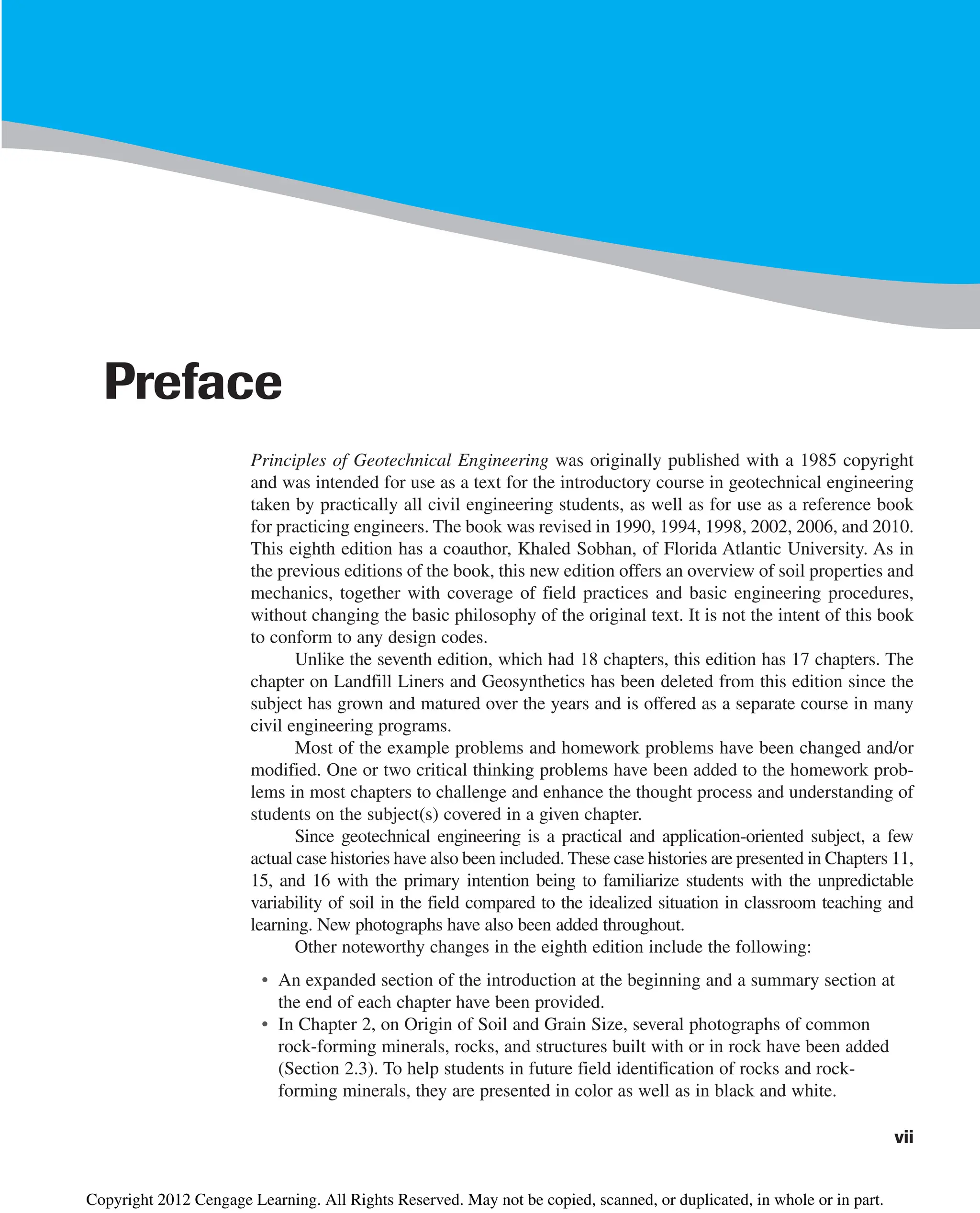
The document provides an overview of the principles of geotechnical engineering. It begins with a historical perspective on the development of the field from ancient times through the modern era. It then covers various topics related to soil properties including the origin and formation of soils, particle size and shape, clay minerals, specific gravity, mechanical analysis, particle size distribution, weight-volume relationships, void ratio, porosity, moisture content, unit weights, and relative density. The text is intended as a textbook for introductory geotechnical engineering courses.


![24 Chapter 2: Origin of Soil and Grain Size
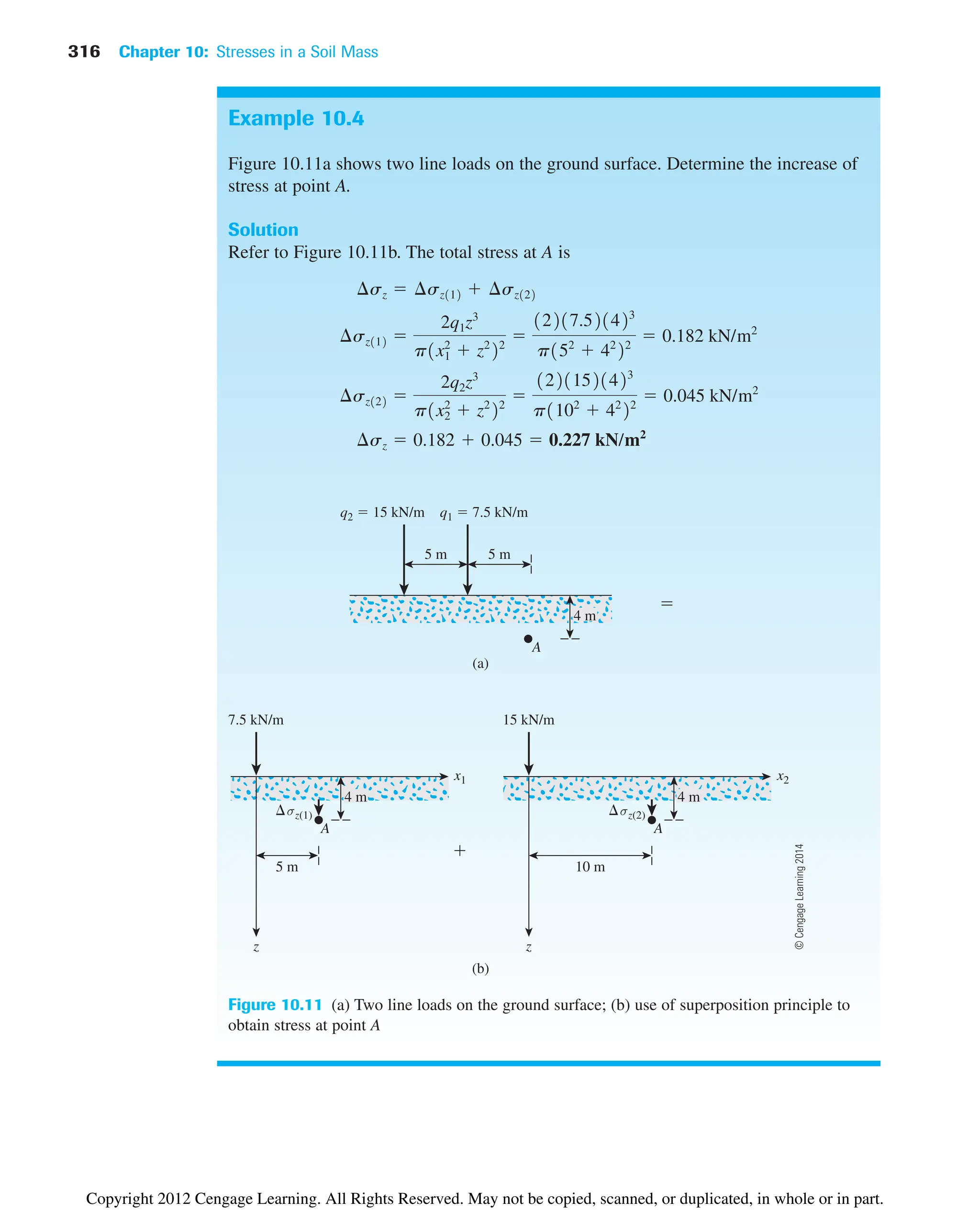
Fine-grained soil is found at the surface, and the grain size increases with depth. At
greater depths, angular rock fragments may also be found.
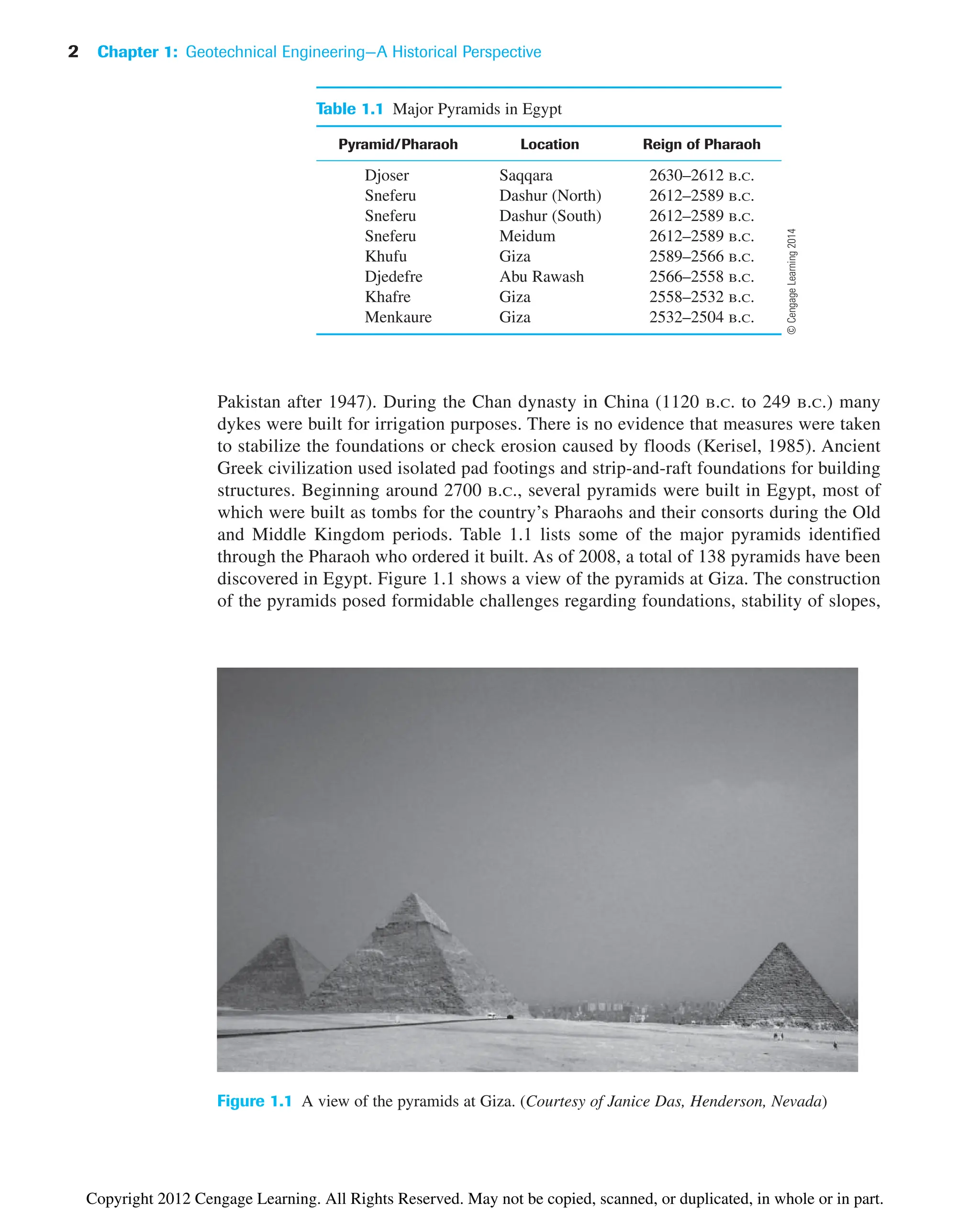
The transported soils may be classified into several groups, depending on their mode
of transportation and deposition:
1. Glacial soils—formed by transportation and deposition of glaciers
2. Alluvial soils—transported by running water and deposited along streams
3. Lacustrine soils—formed by deposition in quiet lakes
4. Marine soils—formed by deposition in the seas
5. Aeolian soils—transported and deposited by wind
6. Colluvial soils—formed by movement of soil from its original place by gravity, such
as during landslides
Sedimentary Rock
The deposits of gravel, sand, silt, and clay formed by weathering may become compacted
by overburden pressure and cemented by agents like iron oxide, calcite, dolomite, and
quartz. Cementing agents are generally carried in solution by groundwater. They fill the
spaces between particles and form sedimentary rock. Rocks formed in this way are called
detrital sedimentary rocks.
All detrital rocks have a clastic texture. The following are some examples of detrital
rocks with clastic texture.
Particle size Sedimentary rock
Granular or larger (grain size 2 mm–4 mm or larger) Conglomerate
Sand Sandstone
Silt and clay Mudstone and shale
In the case of conglomerates, if the particles are more angular, the rock is called breccia.
In sandstone, the particle sizes may vary between mm and 2 mm. When the grains in
sandstone are practically all quartz, the rock is referred to as orthoquartzite. In mudstone
and shale, the size of the particles are generally less than mm. Mudstone has a blocky
aspect; whereas, in the case of shale, the rock is split into platy slabs.
Sedimentary rock also can be formed by chemical processes. Rocks of this type are
classified as chemical sedimentary rock. These rocks can have clastic or nonclastic texture.
The following are some examples of chemical sedimentary rock.
Composition Rock
Calcite (CaCO3) Limestone
Halite (NaCl) Rock salt
Dolomite [CaMg(CO3)] Dolomite
Gypsum (CaSO4 2H2O) Gypsum
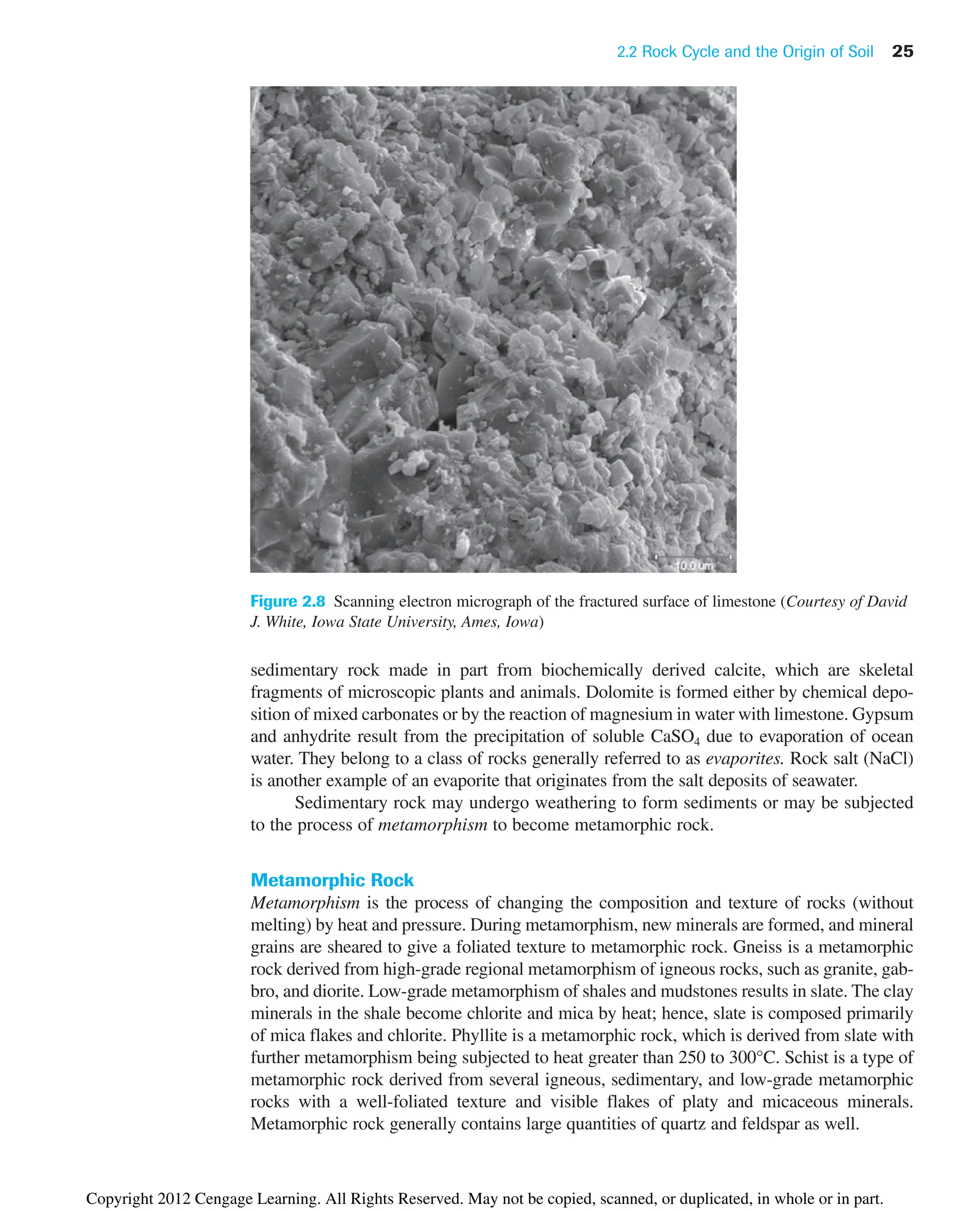
Limestone is formed mostly of calcium carbonate deposited either by organisms or by
an inorganic process. Most limestones have a clastic texture; however, nonclastic textures
also are found commonly. Figure 2.8 shows the scanning electron micrograph of a fractured
surface of limestone. Individual grains of calcite show rhombohedral cleavage. Chalk is a
1
16
1
16
©
Cengage
Learning
2014
©
Cengage
Learning
2014
Copyright 2012 Cengage Learning. All Rights Reserved. May not be copied, scanned, or duplicated, in whole or in part.](https://image.slidesharecdn.com/principlesofgeotechnicalengineering-8thedition-231222125509-7e44d9bf/75/Principles-of-Geotechnical-Engineering-8th-Edition-pdf-44-2048.jpg)

![70 Chapter 3: Weight–Volume Relationships
may sometimes be convenient. The SI unit of mass density is kilograms per cubic meter
(kg/m3
). We can write the density equations [similar to Eqs. (3.9) and (3.11)] as
(3.13)
and
(3.14)
where r density of soil (kg/m3
)
rd dry density of soil (kg/m3
)
M total mass of the soil sample (kg)
Ms mass of soil solids in the sample (kg)
The unit of total volume, V, is m3
.
The unit weight in kN/m3
can be obtained from densities in kg/m3
as
and
where g acceleration due to gravity 9.81 m/sec2
.
Note that unit weight of water (gw) is equal to 9.81 kN/m3
or 1000 kgf/m3
.
3.3 Relationships among Unit Weight,
Void Ratio, Moisture Content,
and Specific Gravity
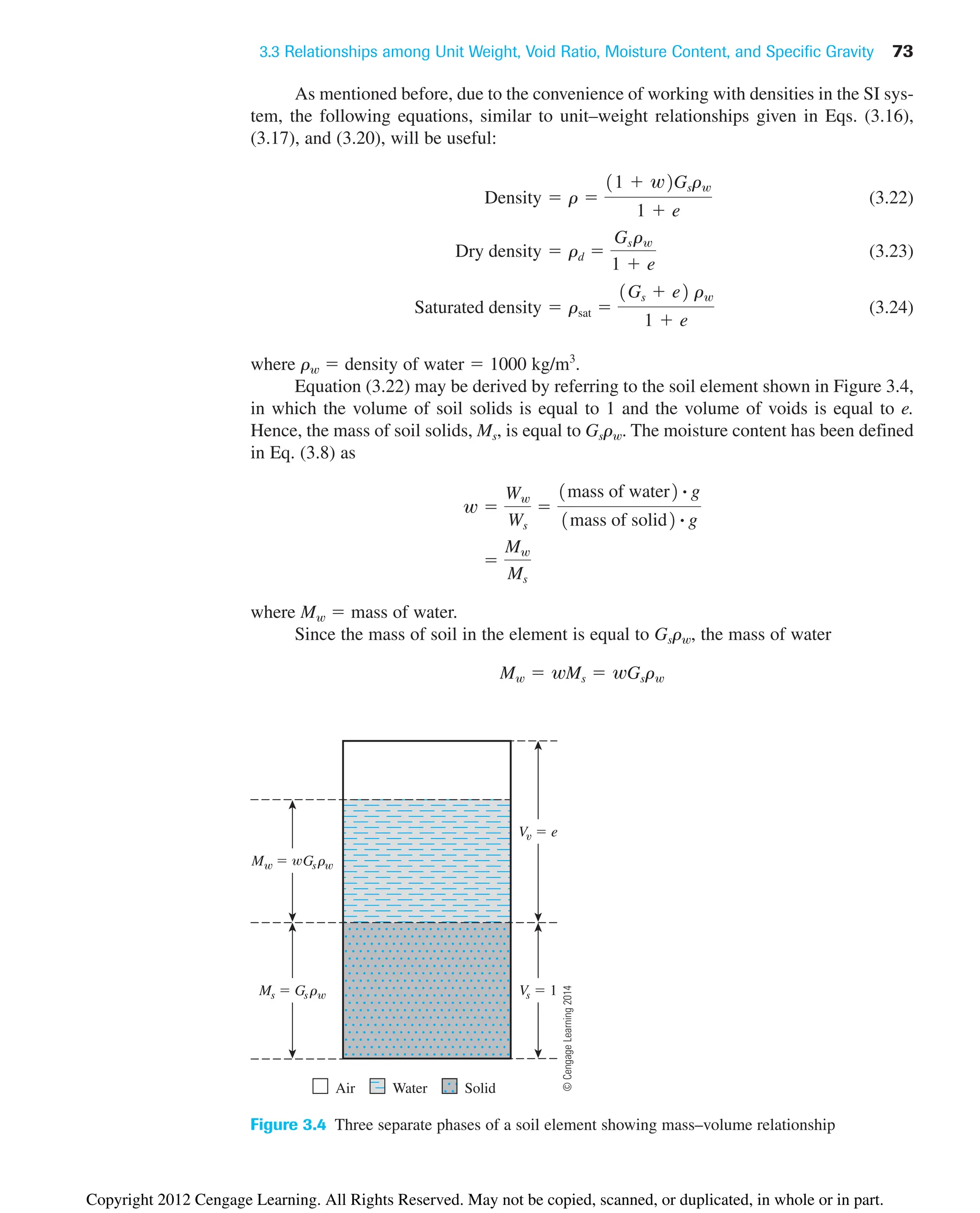
To obtain a relationship among unit weight (or density), void ratio, and moisture content,
let us consider a volume of soil in which the volume of the soil solids is one, as shown in
Figure 3.2. If the volume of the soil solids is 1, then the volume of voids is numerically
equal to the void ratio, e [from Eq. (3.3)]. The weights of soil solids and water can be
given as
where Gs specific gravity of soil solids
w moisture content
gw unit weight of water
Ww wWs wGsgw
Ws Gsgw
gd 1kN/m3
2
grd1kg/m3
2
1000
g 1kN/m3
2
gr1kg/m3
2
1000
rd
Ms
V
r
M
V
Copyright 2012 Cengage Learning. All Rights Reserved. May not be copied, scanned, or duplicated, in whole or in part.](https://image.slidesharecdn.com/principlesofgeotechnicalengineering-8thedition-231222125509-7e44d9bf/75/Principles-of-Geotechnical-Engineering-8th-Edition-pdf-90-2048.jpg)
![3.3 Relationships among Unit Weight, Void Ratio, Moisture Content, and Specific Gravity 71
W
Vs 1
V 1 e
Weight Volume
W Gsg
Ws Gsg
V Gs
V e
Air Water Solid
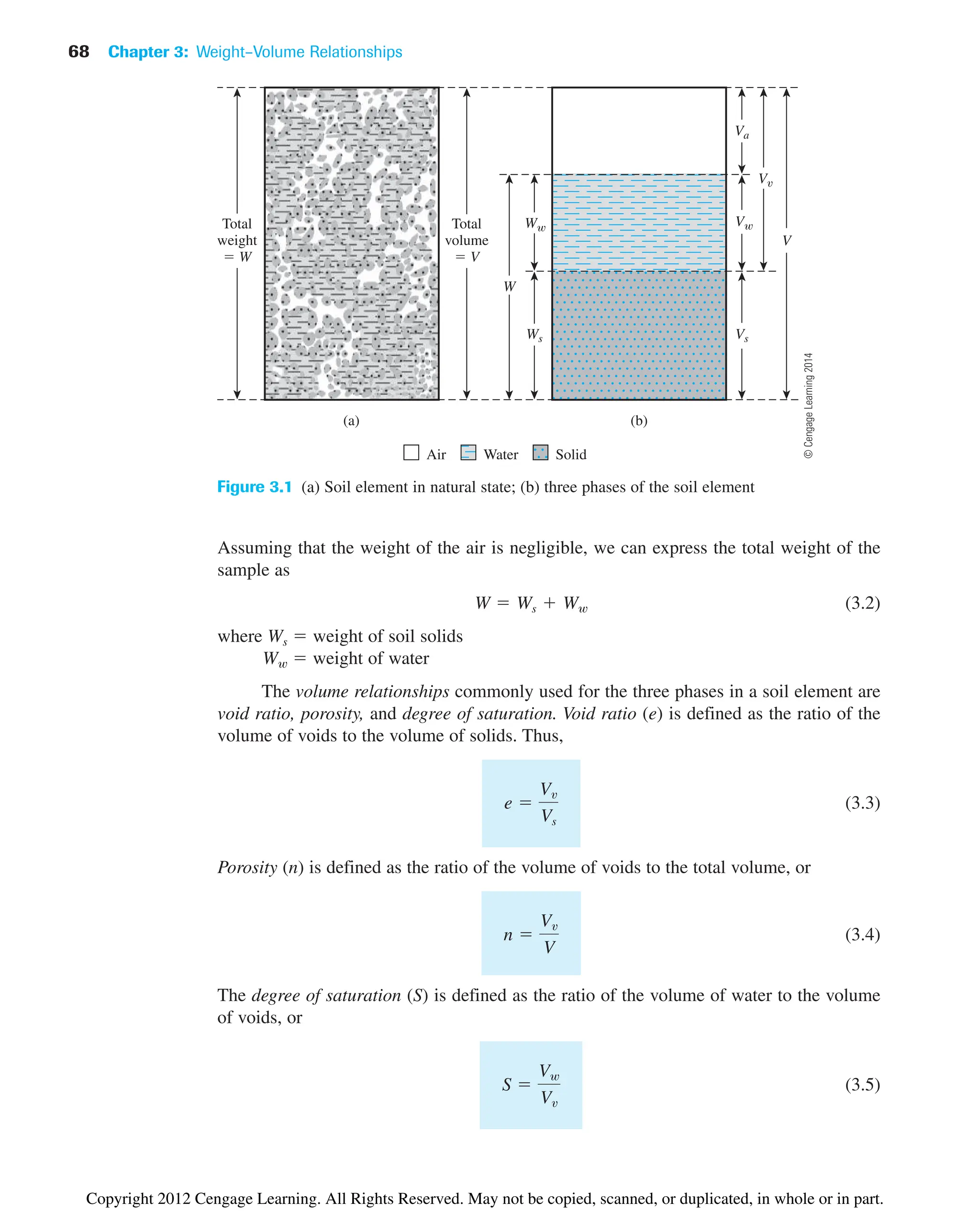
Figure 3.2 Three separate phases of a soil element with volume of soil solids equal to 1
Specific gravity of soil solids (Gs) was defined in Section 2.5 of Chapter 2. It can be
expressed as
(3.15)
Now, using the definitions of unit weight and dry unit weight [Eqs. (3.9) and (3.11)],
we can write
(3.16)
and
(3.17)
or
(3.18)
e
Gsgw
gd
1
gd
Ws
V
Gsgw
1 e
g
W
V
Ws Ww
V
Gsgw wGsgw
1 e
11 w2 Gsgw
1 e
Gs
Ws
Vsgw
©
Cengage
Learning
2014
Copyright 2012 Cengage Learning. All Rights Reserved. May not be copied, scanned, or duplicated, in whole or in part.](https://image.slidesharecdn.com/principlesofgeotechnicalengineering-8thedition-231222125509-7e44d9bf/75/Principles-of-Geotechnical-Engineering-8th-Edition-pdf-91-2048.jpg)
![72 Chapter 3: Weight–Volume Relationships
Because the weight of water for the soil element under consideration is wGsgw, the
volume occupied by water is
Hence, from the definition of degree of saturation [Eq. (3.5)],
or
(3.19)
This equation is useful for solving problems involving three-phase relationships.
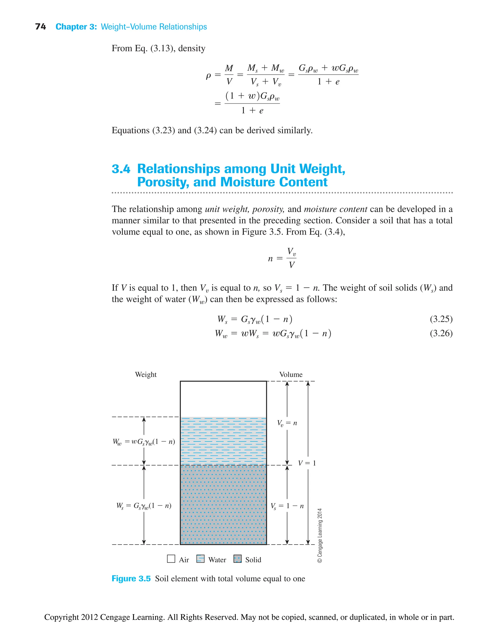
If the soil sample is saturated—that is, the void spaces are completely filled with
water (Figure 3.3)—the relationship for saturated unit weight (gsat) can be derived in a sim-
ilar manner:
(3.20)
Also, from Eq. (3.18) with S 1,
(3.21)
e wGs
gsat
W
V
Ws Ww
V
Gsgw egw
1 e
1Gs e2gw
1 e
Se wGs
S
Vw
Vv
wGs
e
Vw
Ww
gw
wGsgw
gw
wGs
V V e
Ws Gsg
W
Vs 1
V 1 e
Weight Volume
W eg
Water Solid
Figure 3.3 Saturated soil element with volume of soil solids equal to one
©
Cengage
Learning
2014
Copyright 2012 Cengage Learning. All Rights Reserved. May not be copied, scanned, or duplicated, in whole or in part.](https://image.slidesharecdn.com/principlesofgeotechnicalengineering-8thedition-231222125509-7e44d9bf/75/Principles-of-Geotechnical-Engineering-8th-Edition-pdf-92-2048.jpg)
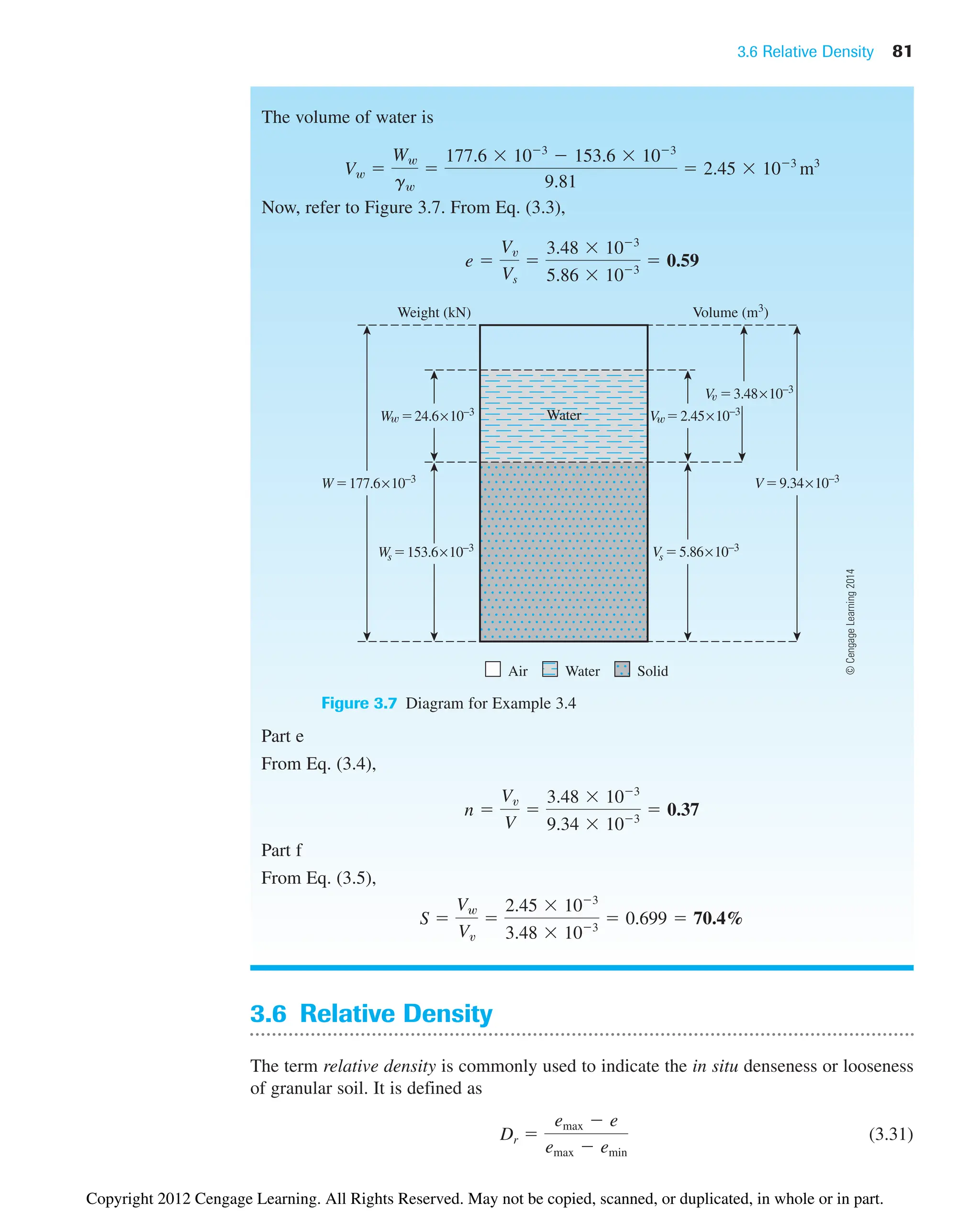
![80 Chapter 3: Weight–Volume Relationships
Example 3.4
In its natural state, a moist soil has a volume of and weighs 177.6
103
kN. The oven-dried weight of the soil is . If , calculate
a. Moisture content (%)
b. Moist unit weight (kN/m3
)
c. Dry unit weight (kN/m3
)
d. Void ratio
e. Porosity
f. Degree of saturation (%)
Solution
Part a
From Eq. (3.8),
Part b
From Eq. (3.9),
Part c
From Eq. (3.11),
Part d
The volume of solids is [Eq. (3.15)]
Thus,
Vv V Vs 9.34 103
5.86 103
3.48 103
m3
Vs
Ws
Gsgw
153.6 103
12.67219.812
5.86 103
m3
gd
Ws
V
153.6 103
9.34 103
16.45 kN/m3
g
W
V
177.6 103
9.34 103
19.01 kN/m3
w
Ww
Ws
177.6 103
153.6 103
153.6 103
11002 15.6%
Gs 2.67
153.6 103
kN
9.34 103
m3
Part c
For saturated conditions,
Therefore,
wsat
Ww
Ws
2.39 103
8.454 103
0.283 or 28.3%
Ww1saturated2 gwVw 19.81210.244 103
2 2.39 103
kN
Vw Vv 0.244 103
m3
.
Vv V Vs 0.562 103
0.318 103
0.244 103
m3
Copyright 2012 Cengage Learning. All Rights Reserved. May not be copied, scanned, or duplicated, in whole or in part.](https://image.slidesharecdn.com/principlesofgeotechnicalengineering-8thedition-231222125509-7e44d9bf/75/Principles-of-Geotechnical-Engineering-8th-Edition-pdf-100-2048.jpg)
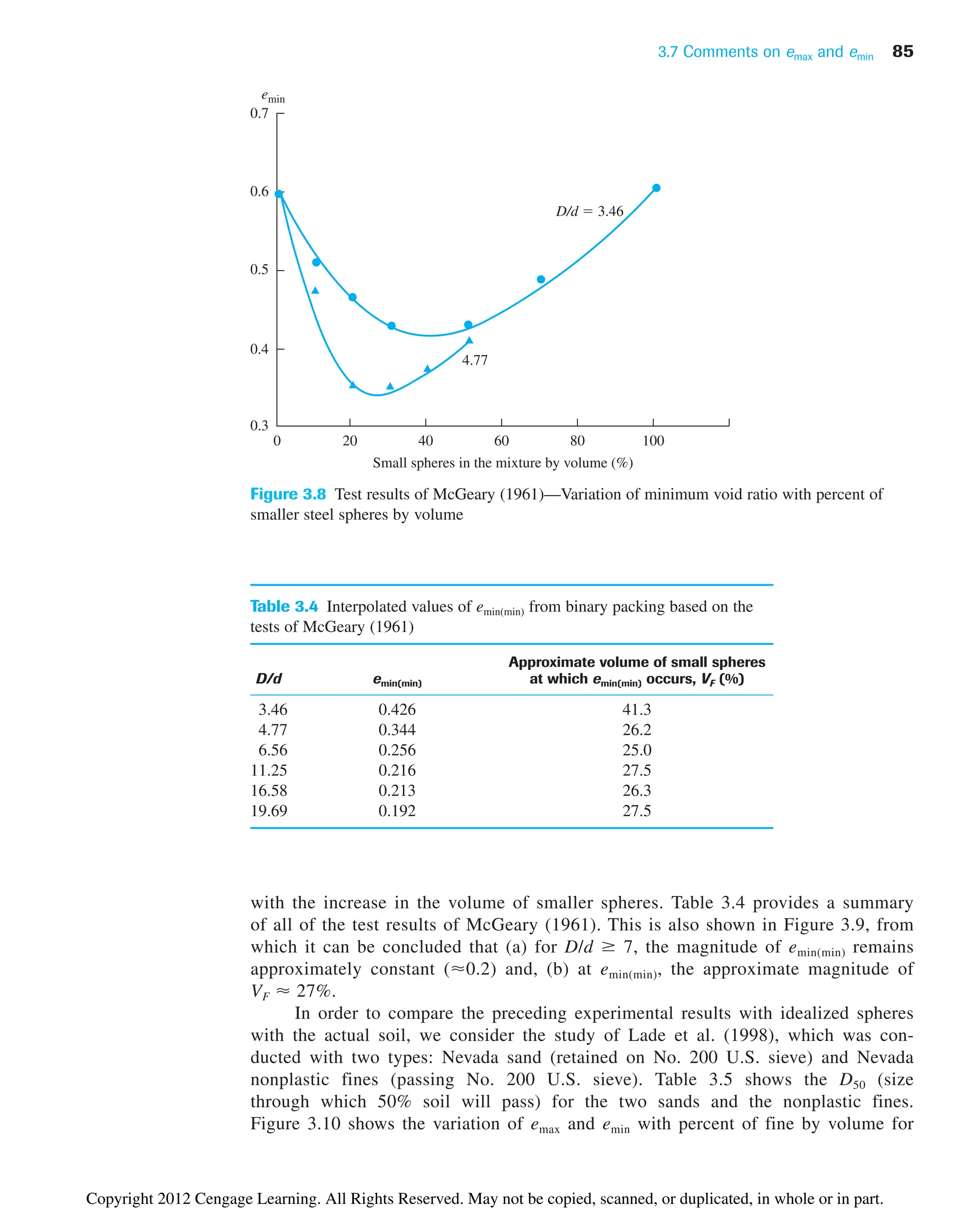
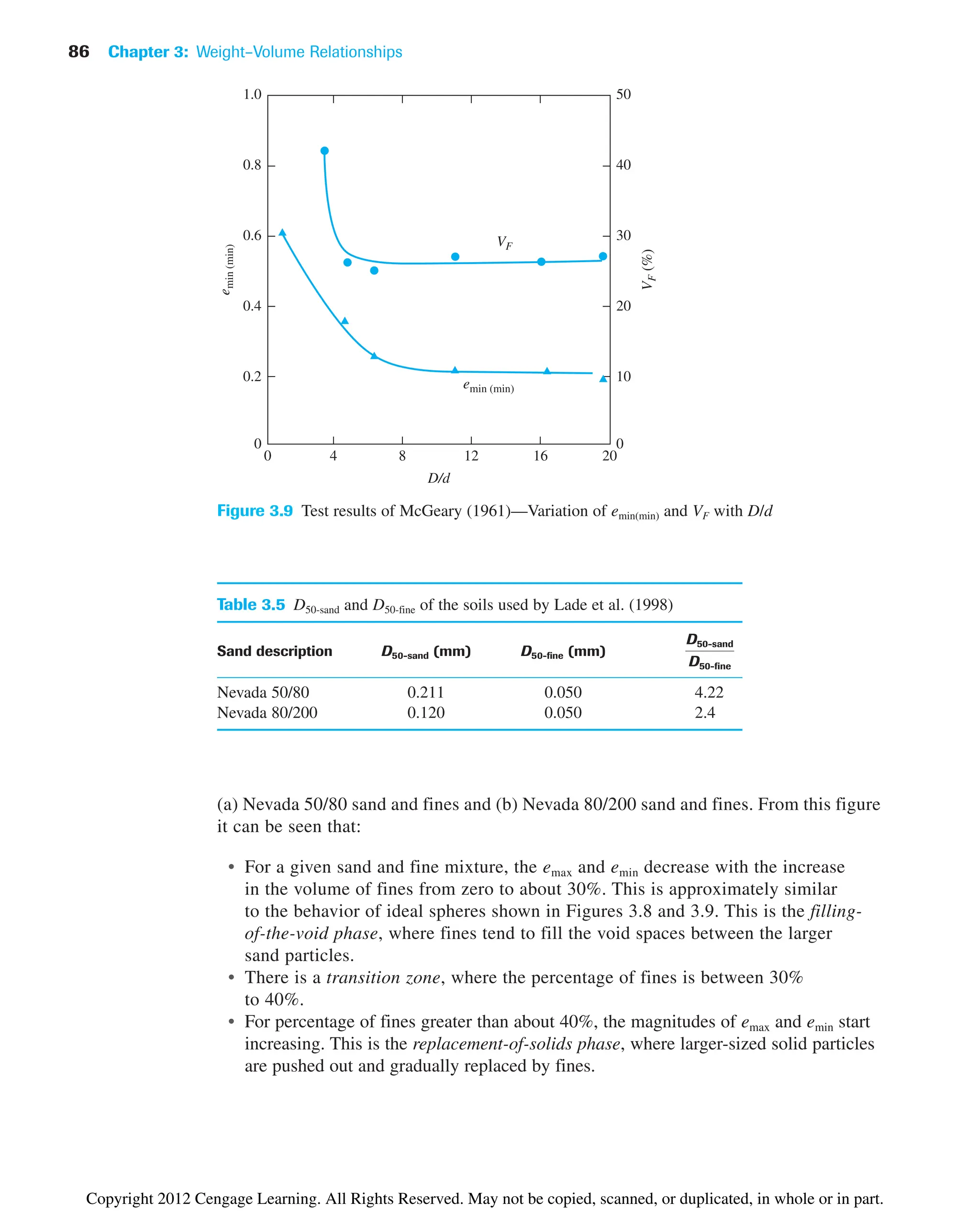
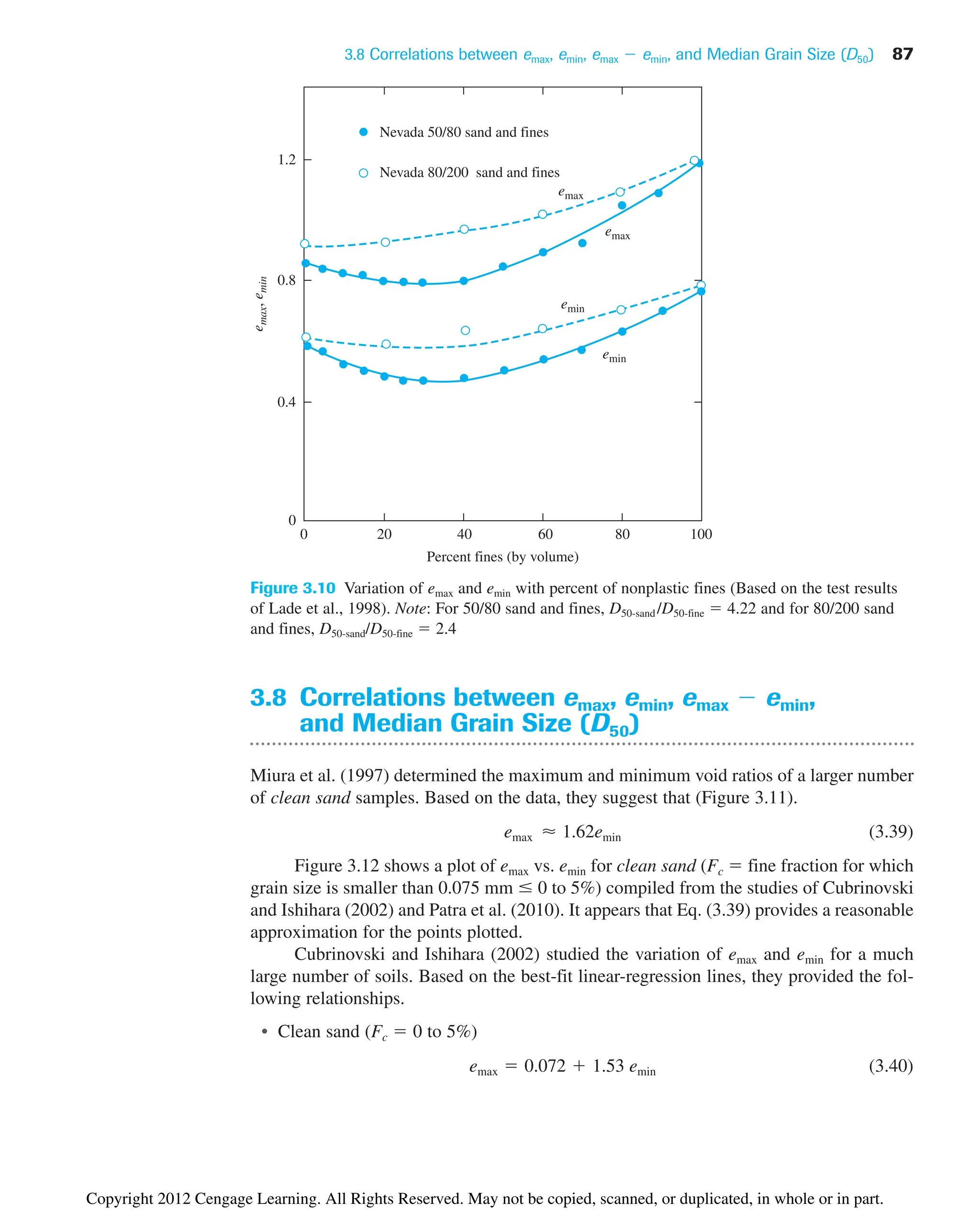
![88 Chapter 3: Weight–Volume Relationships
0.2 0.5 1.0 1.5
Natural sample
Uniform sample
Graded sample
2.0
0.2
0.5
1.0
1.5
2.0
e
max
emin
emax 1.62 emin
emax emin
Figure 3.11 Test results of Miura et al. (1997)—plot of emax vs. emin for clean sand
0.2
0.4
0.5
1.0
1.5
2.0
0.3
Cubrinovski and Ishihara (2002)
Patra et al. (2010)
Eq. (3.39)
0.4 0.5 0.6 0.7 0.8 0.9 1.0
emin
e
max
Figure 3.12 Plot of emax vs. emin for clean sand [Compiled from Cubrinovski and Ishihara (2002);
and Patra, Sivakugan, and Das (2010)]
Copyright 2012 Cengage Learning. All Rights Reserved. May not be copied, scanned, or duplicated, in whole or in part.](https://image.slidesharecdn.com/principlesofgeotechnicalengineering-8thedition-231222125509-7e44d9bf/75/Principles-of-Geotechnical-Engineering-8th-Edition-pdf-108-2048.jpg)
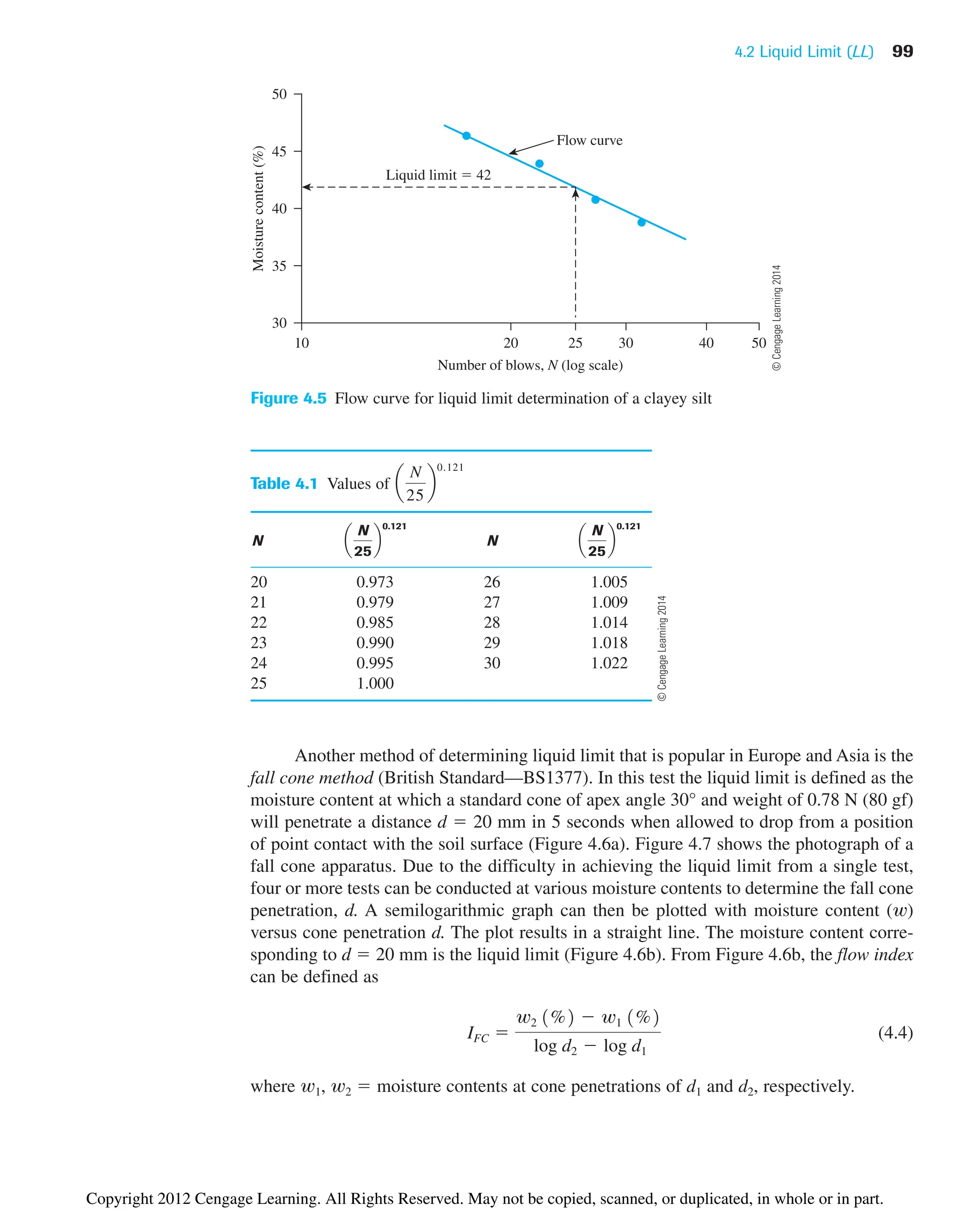
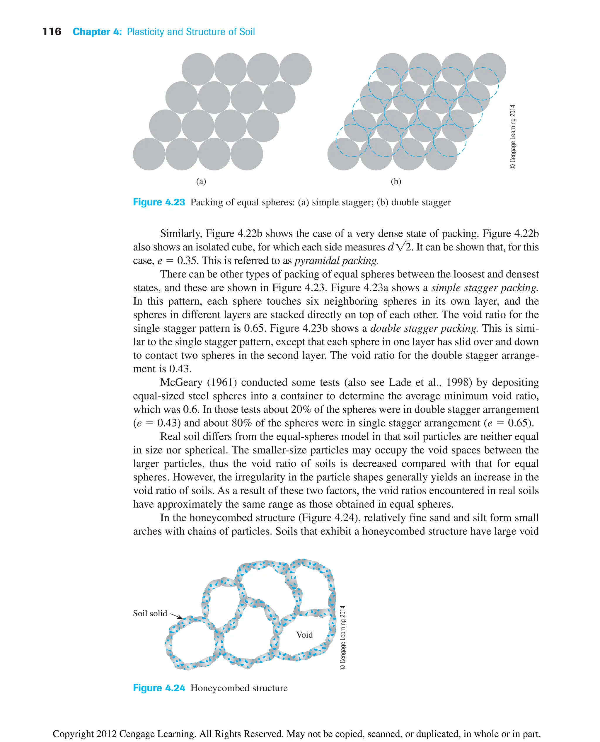
![98 Chapter 4: Plasticity and Structure of Soil
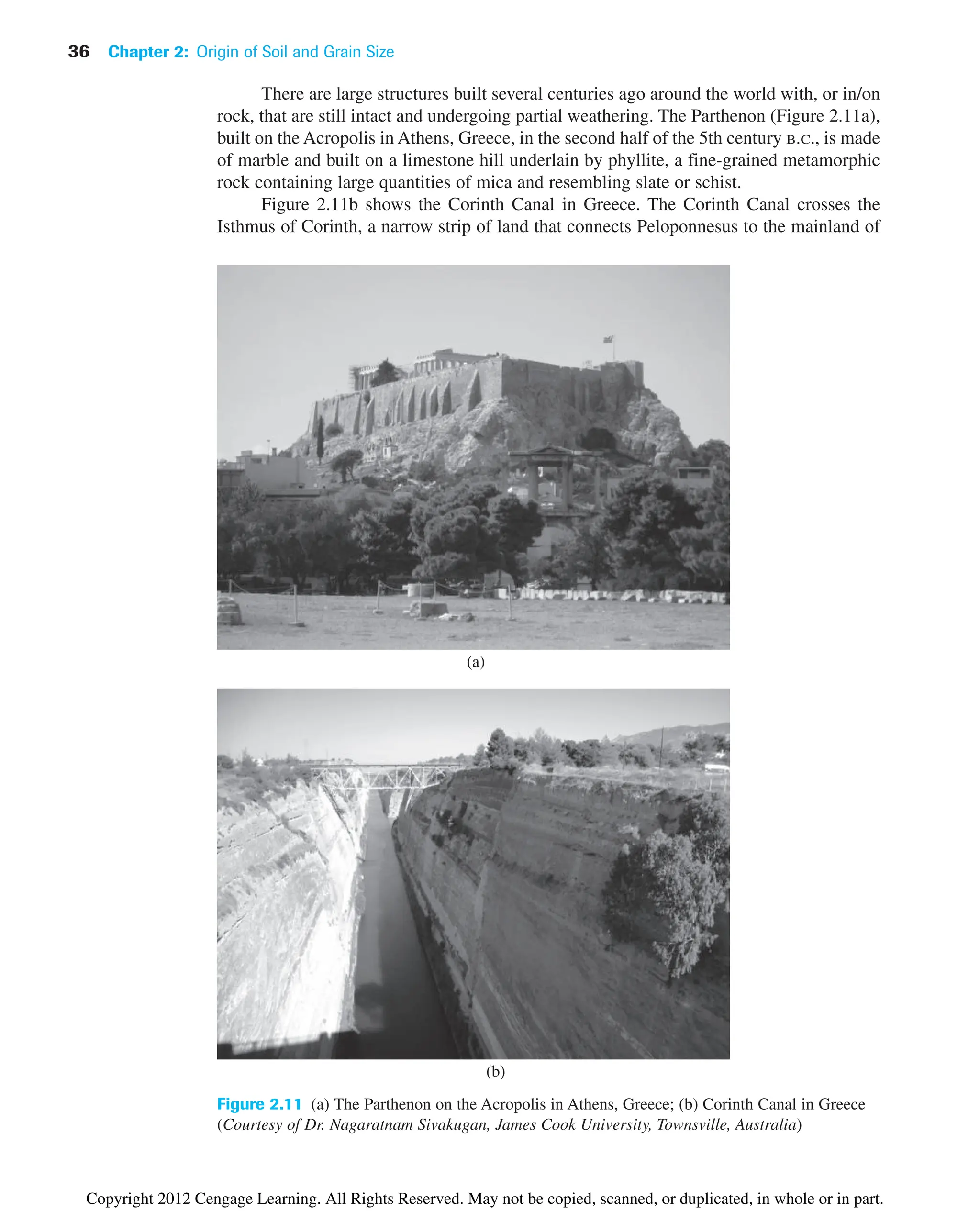
Figure 4.4 Photographs showing the soil pat in the liquid limit device: (a) before test; (b) after
test [Note: The 12.5 mm groove closure in (b) is marked for clarification] (Courtesy of Khaled
Sobhan, Florida Atlantic University, Boca Raton, Florida)
(a)
(b)
Copyright 2012 Cengage Learning. All Rights Reserved. May not be copied, scanned, or duplicated, in whole or in part.](https://image.slidesharecdn.com/principlesofgeotechnicalengineering-8thedition-231222125509-7e44d9bf/75/Principles-of-Geotechnical-Engineering-8th-Edition-pdf-118-2048.jpg)
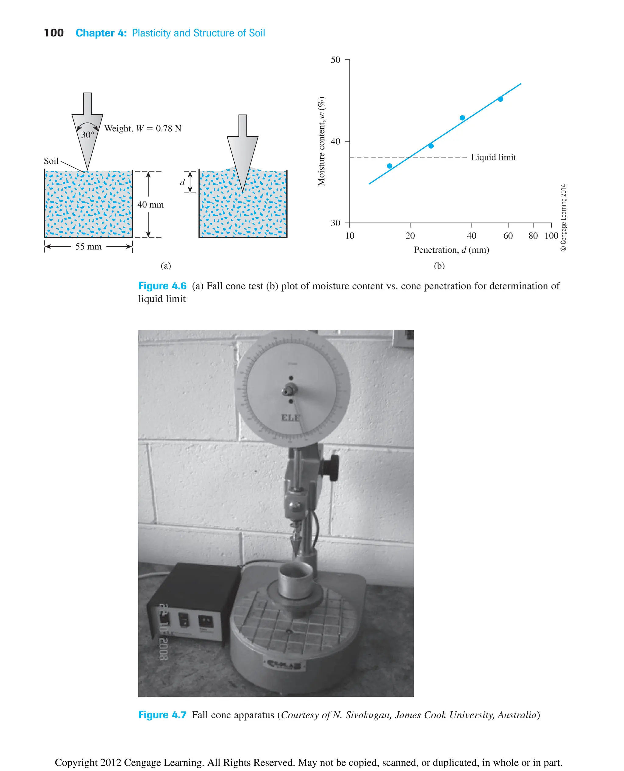
![4.4 Shrinkage Limit (SL) 103
and (Figure 4.10 b)
(4.7)
In a recent study by Polidori (2007) that involved six inorganic soils and their respec-
tive mixtures with fine silica sand, it was shown that
(4.8)
and
(4.9)
where CF clay fraction (2 mm) in %. The experimental results of Polidori (2007)
show that the preceding relationships hold good for CF approximately equal to or greater
than 30%.
4.4 Shrinkage Limit (SL)
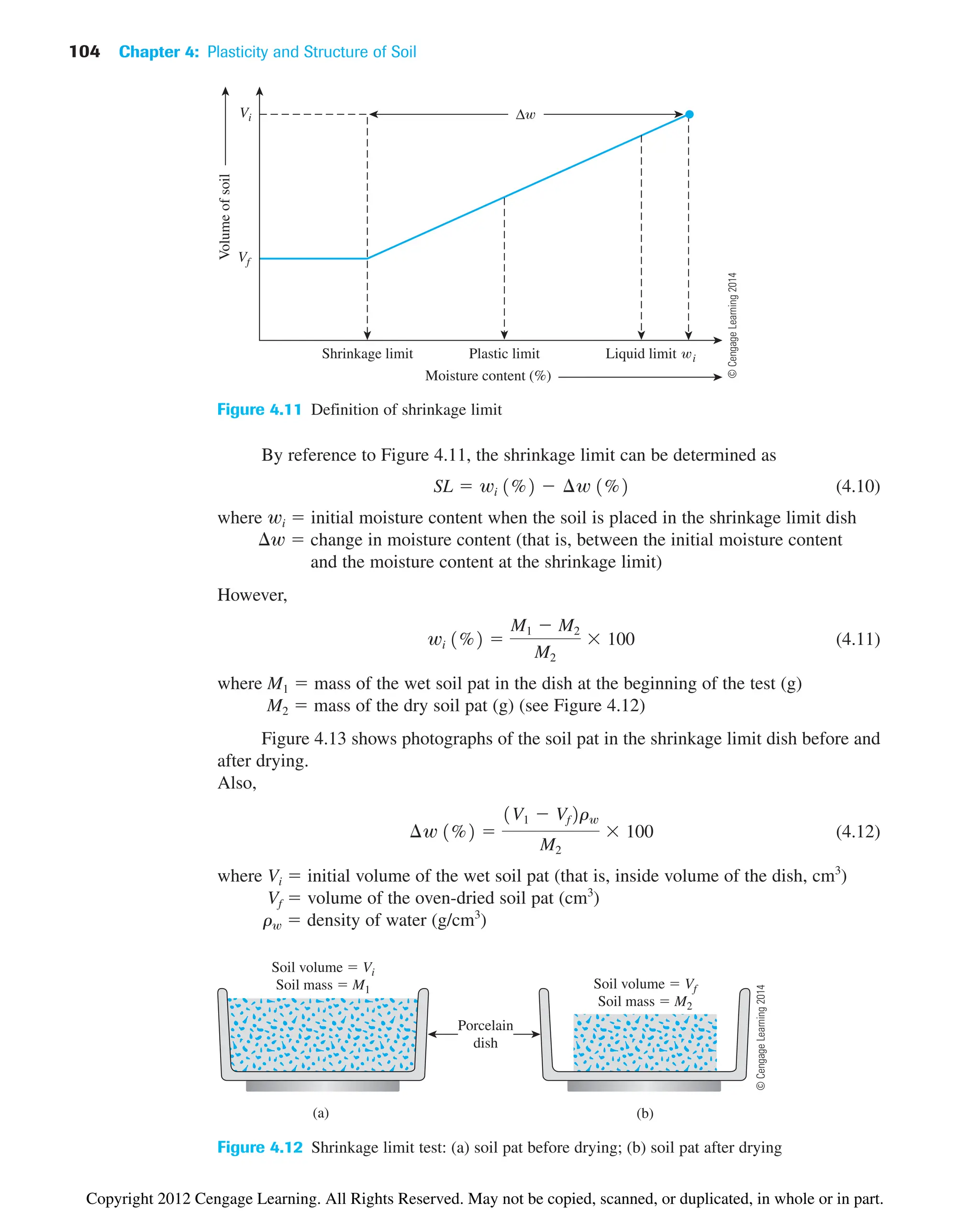
Soil shrinks as moisture is gradually lost from it. With continuing loss of moisture, a stage
of equilibrium is reached at which more loss of moisture will result in no further volume
change (Figure 4.11). The moisture content, in percent, at which the volume of the soil
mass ceases to change is defined as the shrinkage limit.
Shrinkage limit tests [ASTM (2007)—Test Designation D-427] are performed in
the laboratory with a porcelain dish about 44 mm (1.75 in.) in diameter and about 12.7 mm
( in.) high. The inside of the dish is coated with petroleum jelly and is then filled com-
pletely with wet soil. Excess soil standing above the edge of the dish is struck off with a
straightedge. The mass of the wet soil inside the dish is recorded. The soil pat in the dish
is then oven-dried. The volume of the oven-dried soil pat is determined by the displace-
ment of mercury.
1
2
PI 0.961LL2 0.261CF2 10
PL 0.041LL2 0.261CF2 10
PI 1%2 0.74IFC 1%2
10 20 30
(a)
Eq. (4.6)
PI
(%)
40 50 60
0
50
100
150
200
250
0
IF (%)
50 100 150
(b)
Eq. (4.7)
PI
(%)
200 250 300
0
50
100
150
200
0
IFC (%)
Figure 4.10 Variation of PI with (a) IF; and (b) IFC (Adapted after Sridharan et al. (1999). With
permission from ASTM.)
Copyright 2012 Cengage Learning. All Rights Reserved. May not be copied, scanned, or duplicated, in whole or in part.](https://image.slidesharecdn.com/principlesofgeotechnicalengineering-8thedition-231222125509-7e44d9bf/75/Principles-of-Geotechnical-Engineering-8th-Edition-pdf-123-2048.jpg)
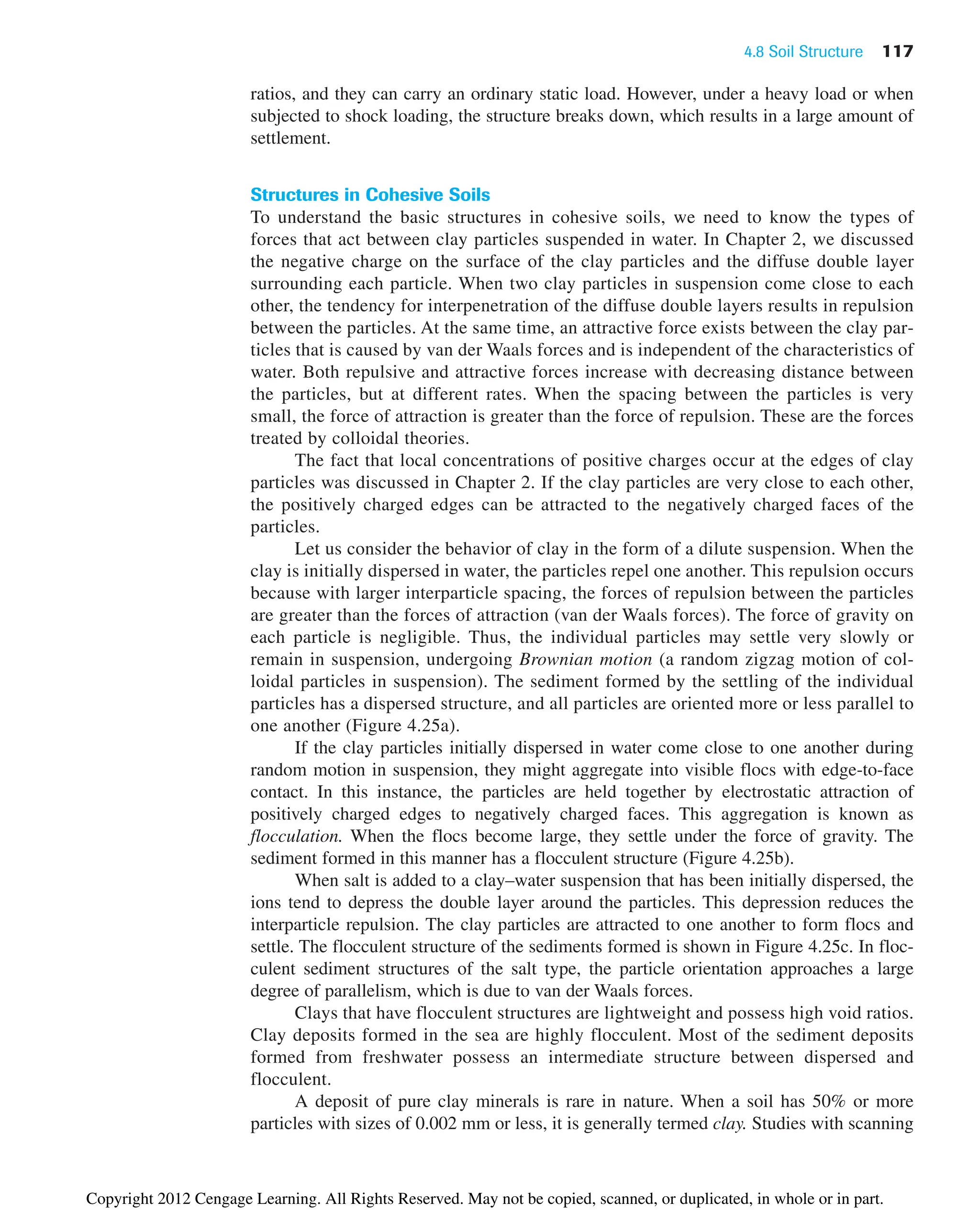
![4.9 Summary 119
Table 4.3 Structure of Clay Soils
Item Remarks
Dispersed structures Formed by settlement of individual clay particles; more or less
parallel orientation (see Figure 4.25a)
Flocculent structures Formed by settlement of flocs of clay particles
(see Figures 4.25b and 4.25c)
Domains Aggregated or flocculated submicroscopic units of clay
particles
Clusters Domains group to form clusters; can be seen under light
microscope
Peds Clusters group to form peds; can be seen without microscope
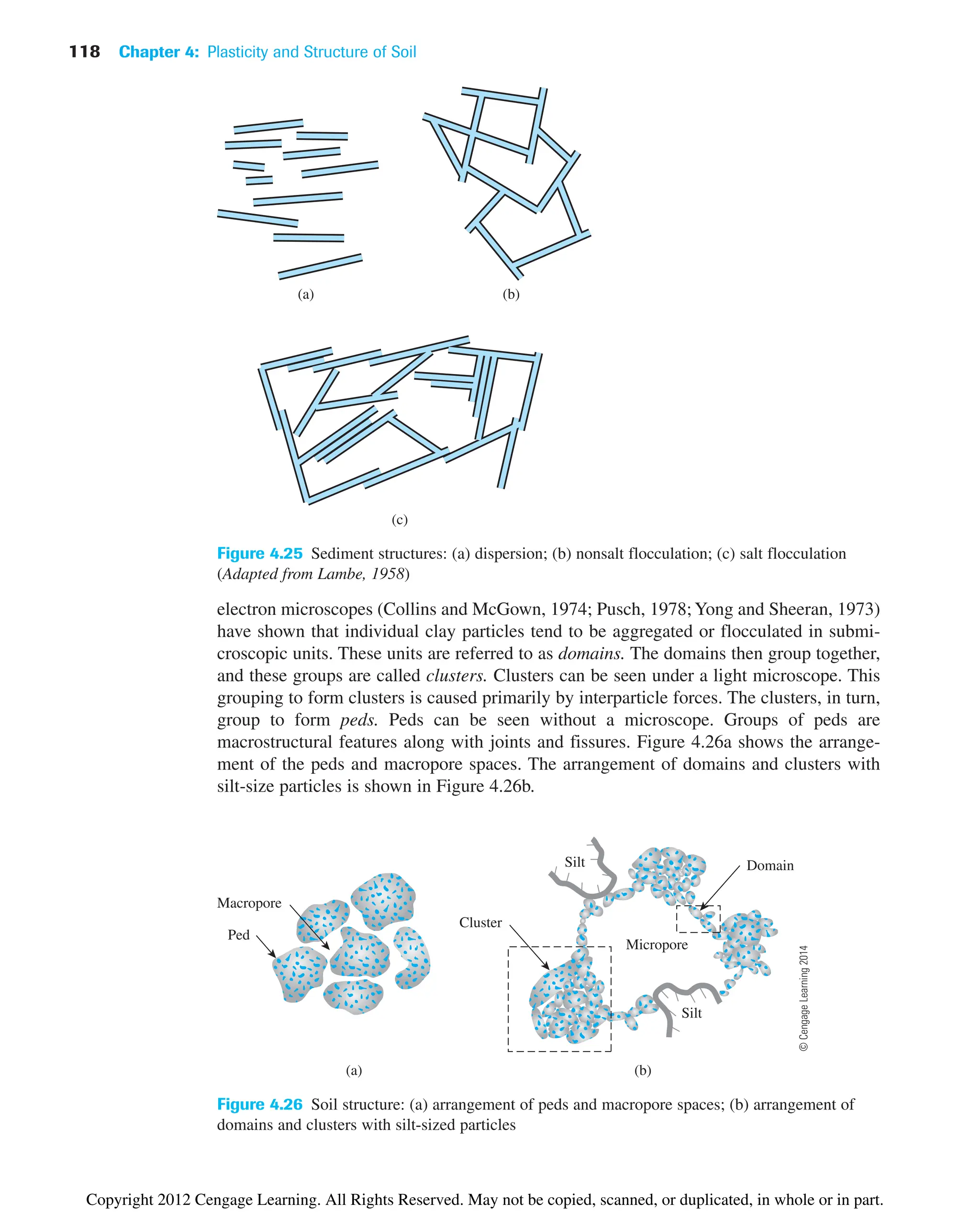
From the preceding discussion, we can see that the structure of cohesive soils is
highly complex. Macrostructures have an important influence on the behavior of soils from
an engineering viewpoint. The microstructure is more important from a fundamental
viewpoint. Table 4.3 summarizes the macrostructures of clay soils.
4.9 Summary
Following is a summary of the materials presented in this chapter.
• The consistency of fine-grained soils can be described by three parameters: the
liquid limit, plastic limit, and shrinkage limit. These are referred to as Atterberg
limits.
• The liquid (LL), plastic (PL), and shrinkage (SL) limits are, respectively, the moisture
contents (%) at which the consistency of soil changes from liquid to plastic stage,
plastic to semisolid stage, and semisolid to solid stage.
• Plasticity index (PI) is the difference between the liquid limit (LL) and the plastic
limit (PL) [Eq. (4.5)].
• Liquidity index of soil (LI) is the ratio of the difference between the in situ moisture
content (%) and the plastic limit to the plasticity index [Eq. (4.24)], or
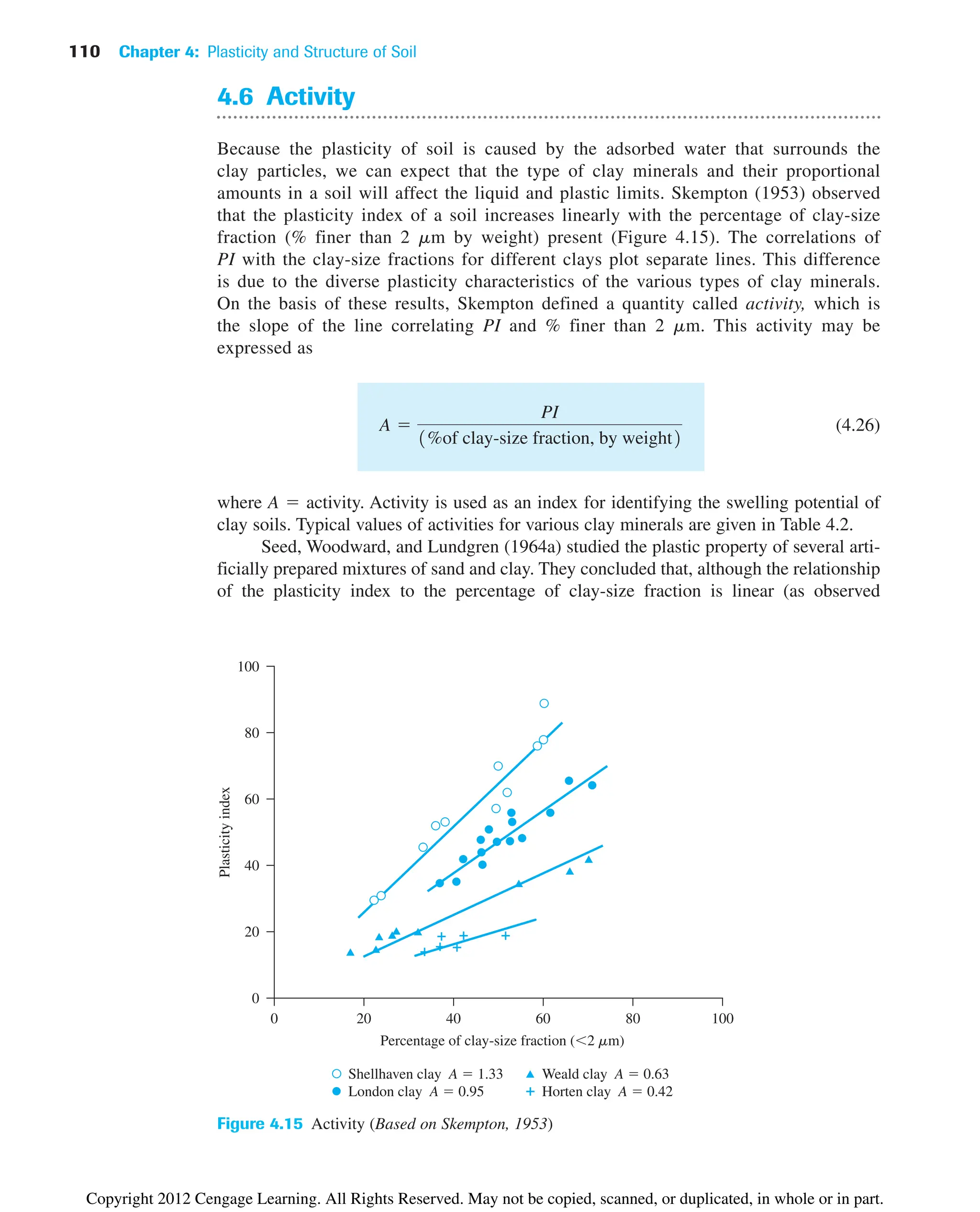
• Activity, A, is defined as the ratio of plasticity index to the percent of clay-size
fraction by weight in a soil [Eq. (4.26)].
• The structure of cohesionless soils can be single grained or honeycombed. Soils with
honeycombed structure have large void ratios that may break down under heavy load
and dynamic loading.
• Dispersion, nonsalt flocculation, and salt flocculation of clay soils were discussed in
Section 4.8. Also discussed in this section is the structure of fine-grained soil as it
relates to the arrangement of peds and micropore spaces and the arrangement of
domains and clusters with silt-size particles.
LI
w PL
LL PL
©
Cengage
Learning
2014
Copyright 2012 Cengage Learning. All Rights Reserved. May not be copied, scanned, or duplicated, in whole or in part.](https://image.slidesharecdn.com/principlesofgeotechnicalengineering-8thedition-231222125509-7e44d9bf/75/Principles-of-Geotechnical-Engineering-8th-Edition-pdf-139-2048.jpg)
![120 Chapter 4: Plasticity and Structure of Soil
Problems
4.1 Results from liquid and plastic limit tests conducted on a soil are given below.
Liquid limit tests:
Number of blows, N Moisture content (%)
14 38.4
16 36.5
20 33.1
28 27.0
Plastic limit tests: PL 13.4%
a. Draw the flow curve and obtain the liquid limit.
b. What is the plasticity index of the soil?
4.2 Determine the liquidity index of the soil in Problem 4.1 if win situ 32%
4.3 Results from liquid and plastic limit tests conducted on a soil are given below.
Liquid limit tests:
Number of blows, N Moisture content (%)
13 33
18 27
29 22
Plastic limit tests: PL 19.1%
a. Draw the flow curve and obtain the liquid limit.
b. What is the plasticity index of the soil?
4.4 Determine the liquidity index of the soil in Problem 4.3 if win situ 21%
4.5 A saturated soil used to determine the shrinkage limit has initial volume
Vi 20.2 cm3
, final volume Vf 14.3 cm3
, mass of wet soil M1 34 g, and mass
of dry soil M2 24 g. Determine the shrinkage limit and the shrinkage ratio.
4.6 Repeat Problem 4.5 with the following data: Vi 16.2; Vf 10.8 cm3
; M1 44.6 g,
and mass of dry soil, M2 32.8 g.
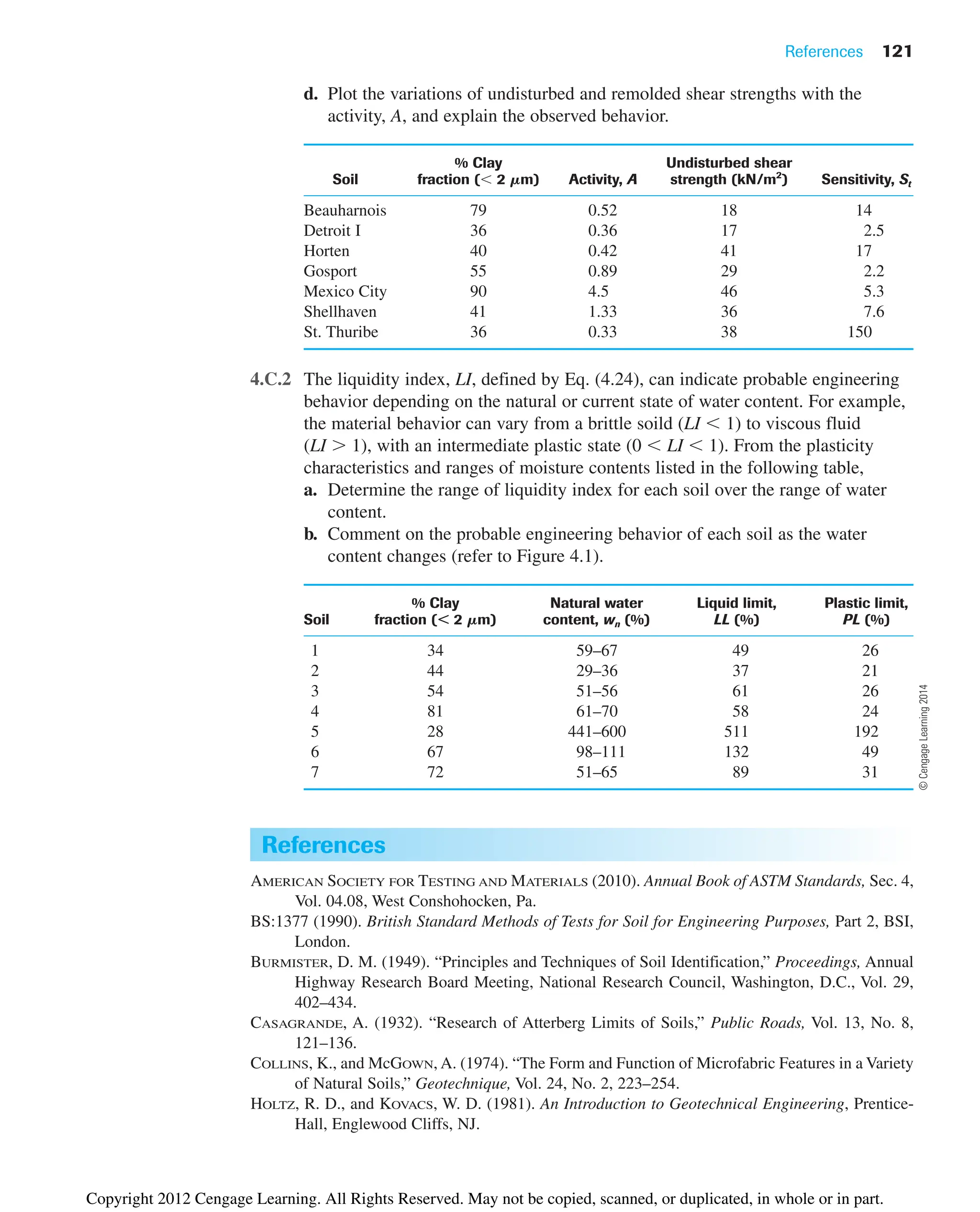
Critical Thinking Problems
4.C.1 The properties of seven different clayey soils are shown below (Skempton and
Northey, 1952). Investigate the relationship between the strength and plasticity
characteristics by performing the following tasks:
a. Estimate the plasticity index for each soil using Skempton’s definition of
activity [Eq. (4.26)].
b. Estimate the probable mineral composition of the clay soils based on PI and A
(use Table 4.2).
c. Sensitivity (St) refers to the loss of strength when the soil is remolded or
disturbed. It is defined as the ratio of the undisturbed strength (tf -undisturbed) to
the remolded strength (tf -remolded) at the same moisture content [Eq. (12.38)].
From the given data, estimate tf -remolded for the clay soils.
©
Cengage
Learning
2014
©
Cengage
Learning
2014
Copyright 2012 Cengage Learning. All Rights Reserved. May not be copied, scanned, or duplicated, in whole or in part.](https://image.slidesharecdn.com/principlesofgeotechnicalengineering-8thedition-231222125509-7e44d9bf/75/Principles-of-Geotechnical-Engineering-8th-Edition-pdf-140-2048.jpg)
![5.4 AASHTO Classification System 129
The first term of Eq. (5.1)—that is, (F200 35)[0.2 0.005(LL 40)]—is the par-
tial group index determined from the liquid limit. The second term—that is,
0.01(F200 15)(PI 10)—is the partial group index determined from the plasticity
index. Following are some rules for determining the group index:
1. If Eq. (5.1) yields a negative value for GI, it is taken as 0.
2. The group index calculated from Eq. (5.1) is rounded off to the nearest whole num-
ber (for example, GI 3.4 is rounded off to 3; GI 3.5 is rounded off to 4).
3. There is no upper limit for the group index.
4. The group index of soils belonging to groups A-1-a, A-1-b, A-2-4, A-2-5, and A-3 is
always 0.
5. When calculating the group index for soils that belong to groups A-2-6 and A-2-7,
use the partial group index for PI, or
(5.2)
In general, the quality of performance of a soil as a subgrade material is inversely propor-
tional to the group index.
GI 0.011F200 1521PI 102
Example 5.2
The results of the particle-size analysis of a soil are as follows:
• Percent passing the No. 10 sieve 42
• Percent passing the No. 40 sieve 35
• Percent passing the No. 200 sieve 20
The liquid limit and plasticity index of the minus No. 40 fraction of the soil are 25
and 20, respectively. Classify the soil by the AASHTO system.
Solution
Since 20% (i.e., less than 35%) of soil is passing No. 200 sieve, it is a granular soil.
Hence it can be A-1, A-2, or A-3. Refer to Table 5.1. Starting from the left of the
table, the soil falls under A-1-b (see the table below).
Parameter Specifications in Table 5.1 Parameters of the given soil
Percent passing sieve
No. 10 —
No. 40 50 max 35
No. 200 25 max 20
Plasticity index (PI) 6 max PI LL PL 25 20 5
The group index of the soil is 0. So, the soil is A-1-b(0).
©
Cengage
Learning
2014
Copyright 2012 Cengage Learning. All Rights Reserved. May not be copied, scanned, or duplicated, in whole or in part.](https://image.slidesharecdn.com/principlesofgeotechnicalengineering-8thedition-231222125509-7e44d9bf/75/Principles-of-Geotechnical-Engineering-8th-Edition-pdf-149-2048.jpg)
![142 Chapter 5: Classification of Soil
5.7 Summary
In this chapter we have discussed the following:
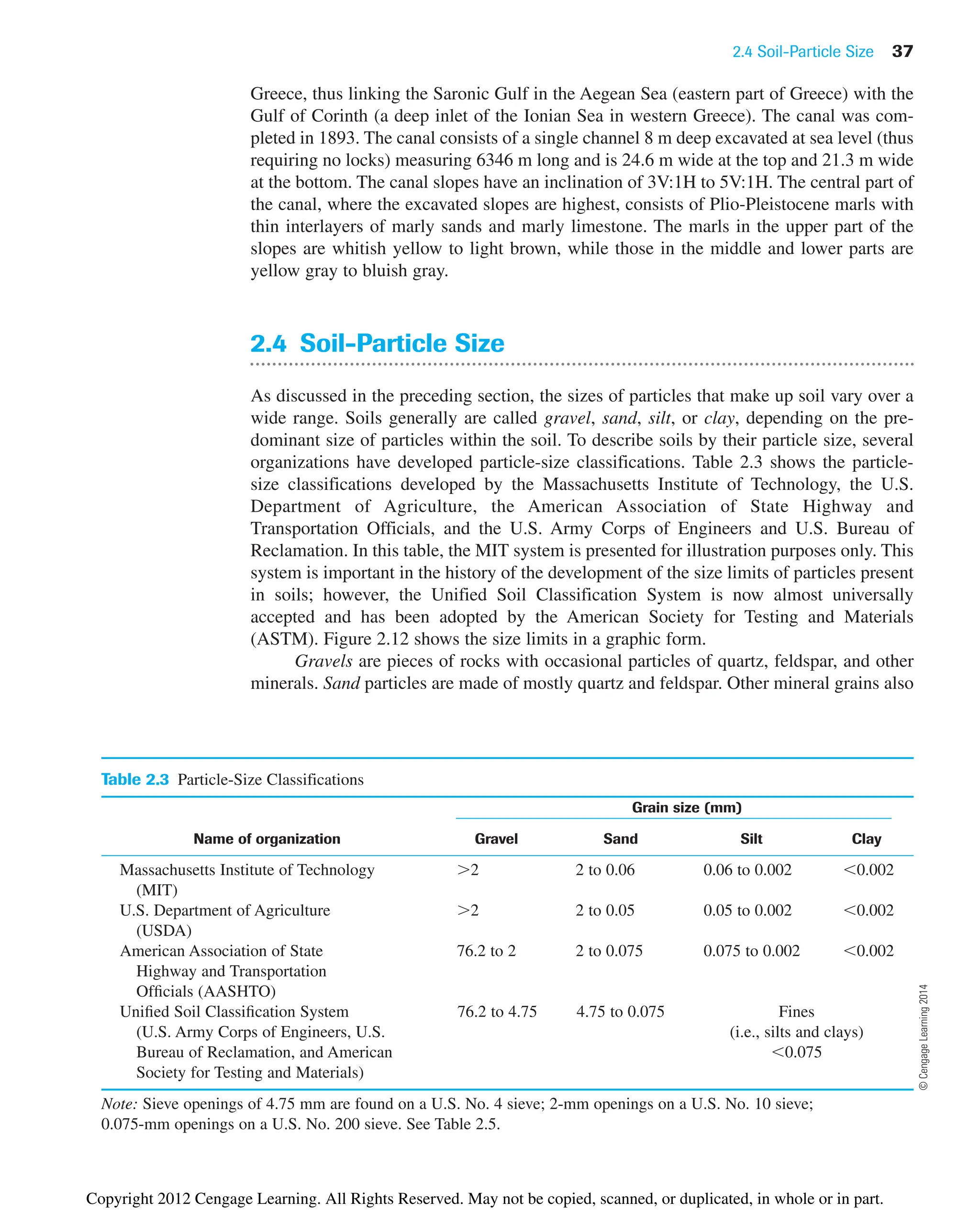
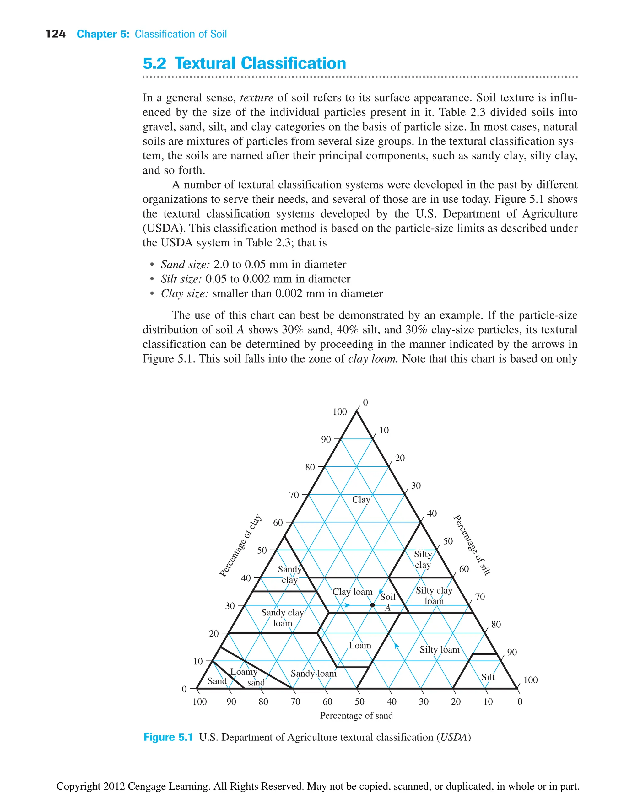
1. Textural classification is based on naming soils based on their principal compo-
nents such as sand, silt, and clay-size fractions determined from particle-size
distribution. The USDA textural classification system is described in detail in
Section 5.2.
2. The AASHTO soil classification system is based on sieve analysis (i.e., percent finer
than No. 10, 40, and 200 sieves), liquid limit, and plasticity index (Table 5.1). Soils
can be classified under categories
• A-1, A-2, and A-3 (granular soils)
• A-4, A-5, A-6, and A-7 (silty and clayey soils)
Group index [Eqs. (5.1) and (5.2)] is added to the soil classification which evaluates
the quality of soil as a subgrade material.
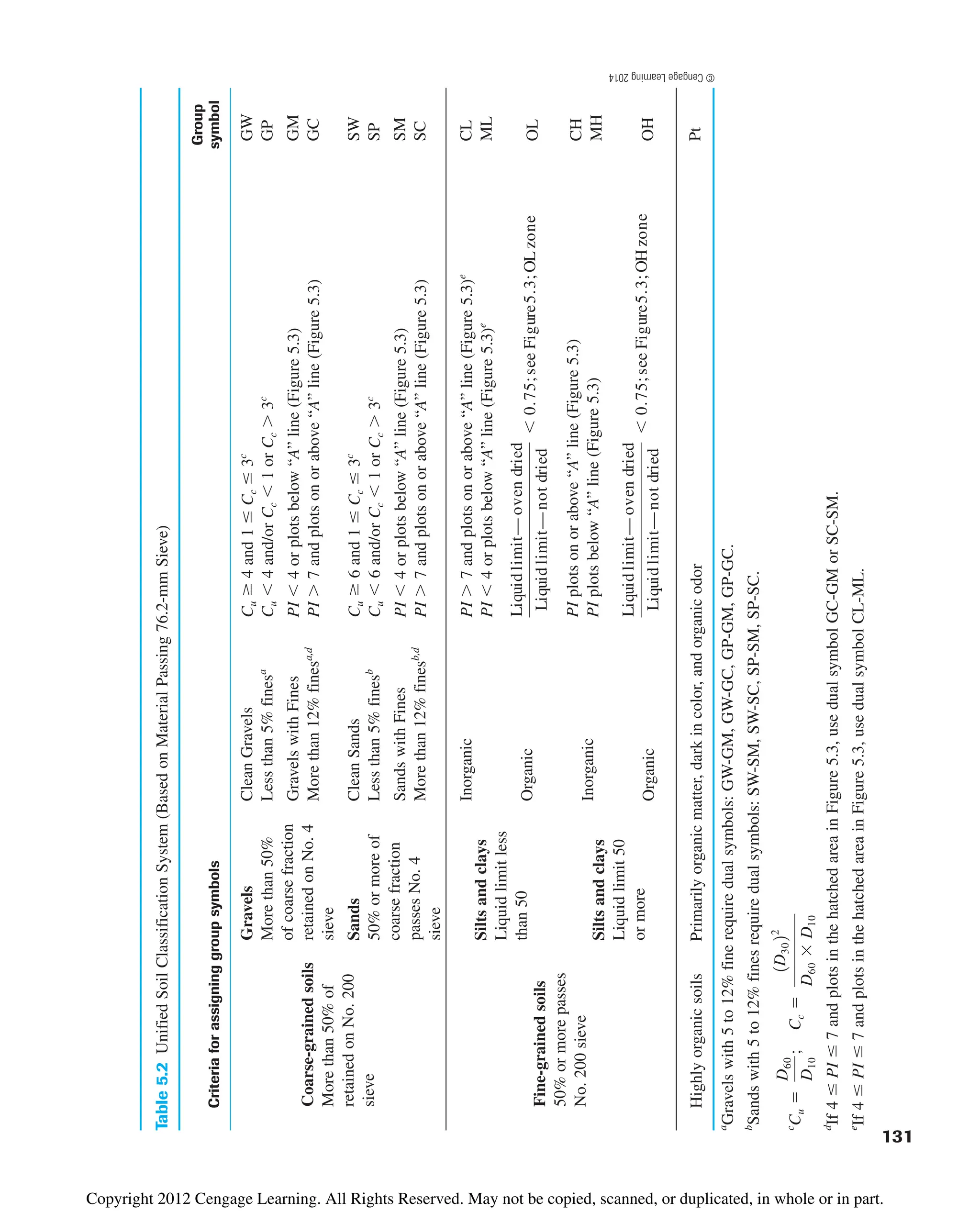
3. Unified soil classification is based on sieve analysis (i.e., percent finer than No. 4
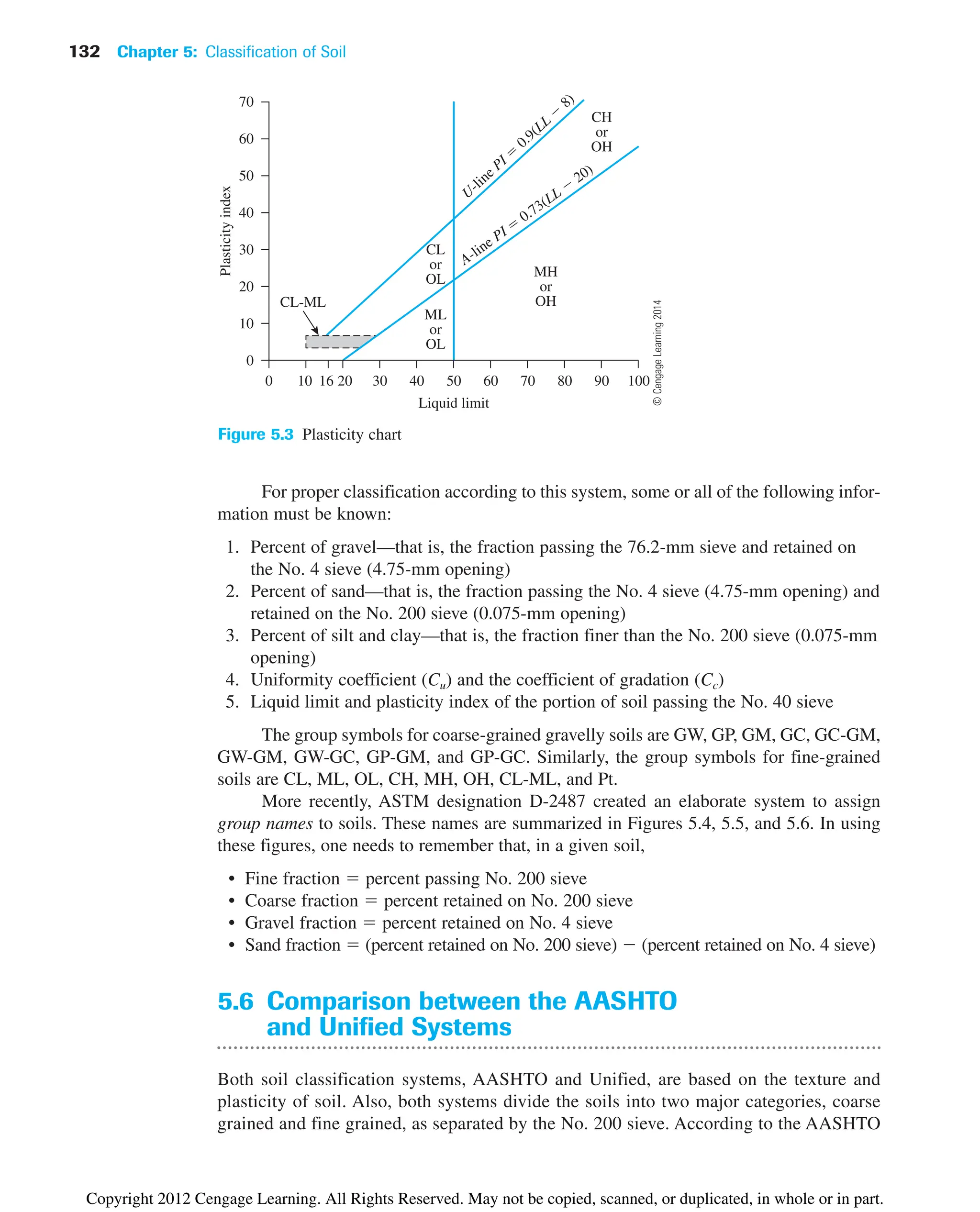
and No. 200 sieves), liquid limit, and plasticity index (Table 5.2 and Figure 5.3). It
uses classification symbols such as
• GW, GP, GM, GC, GW-GM, GW-GC, GP-GM, GP-GC, GC-GM, SW,
SP, SM, SC, SW-SM, SW-SC, SP-SM, SP-SC, and SC-SM (for coarse-grained
soils)
• CL, ML, CL-ML, OL, CH, MH, and OH (for fine-grained soils)
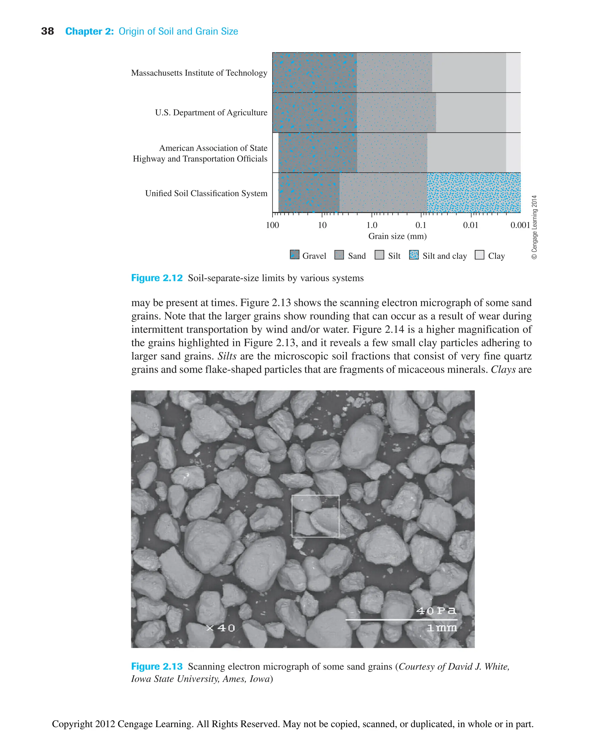
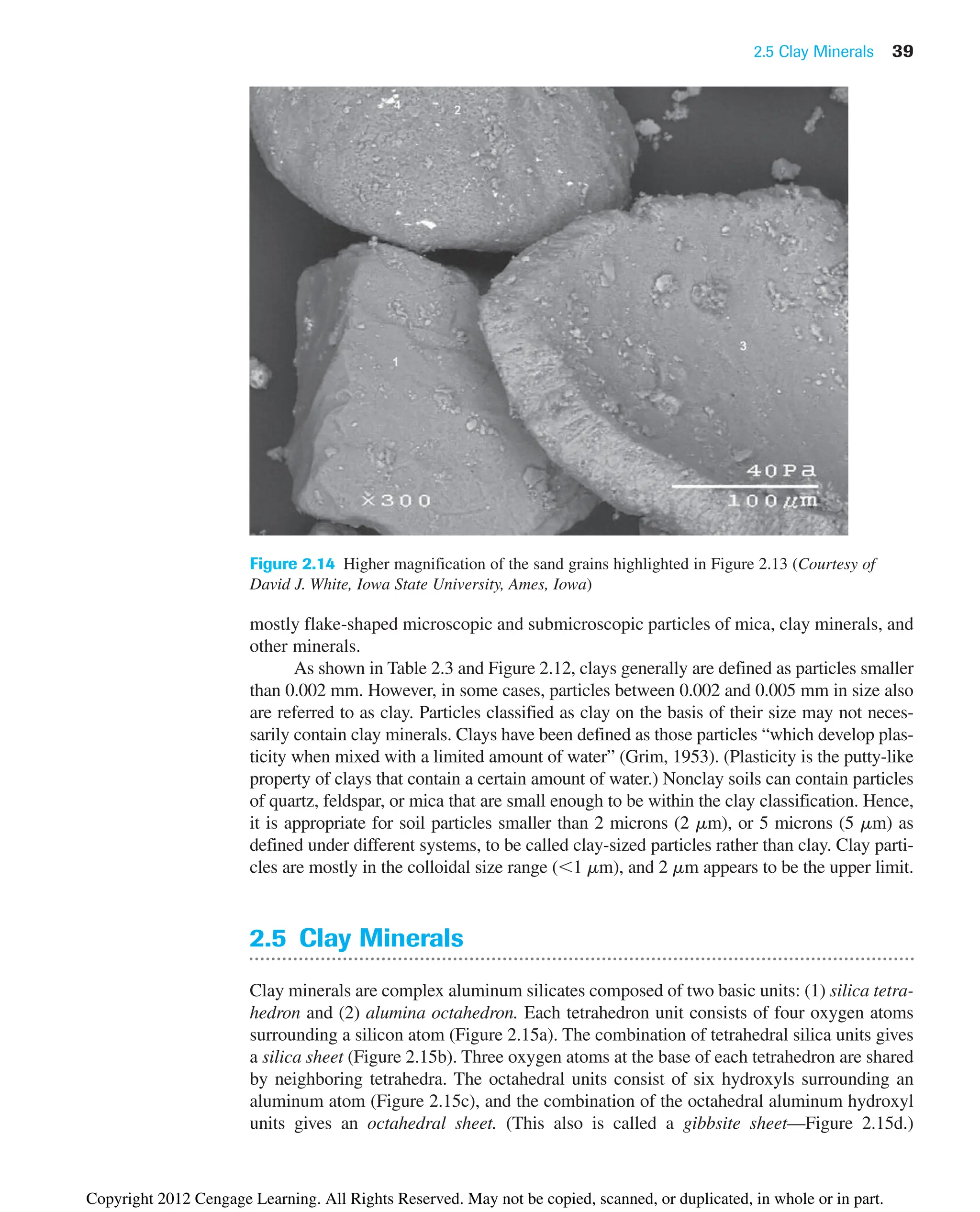
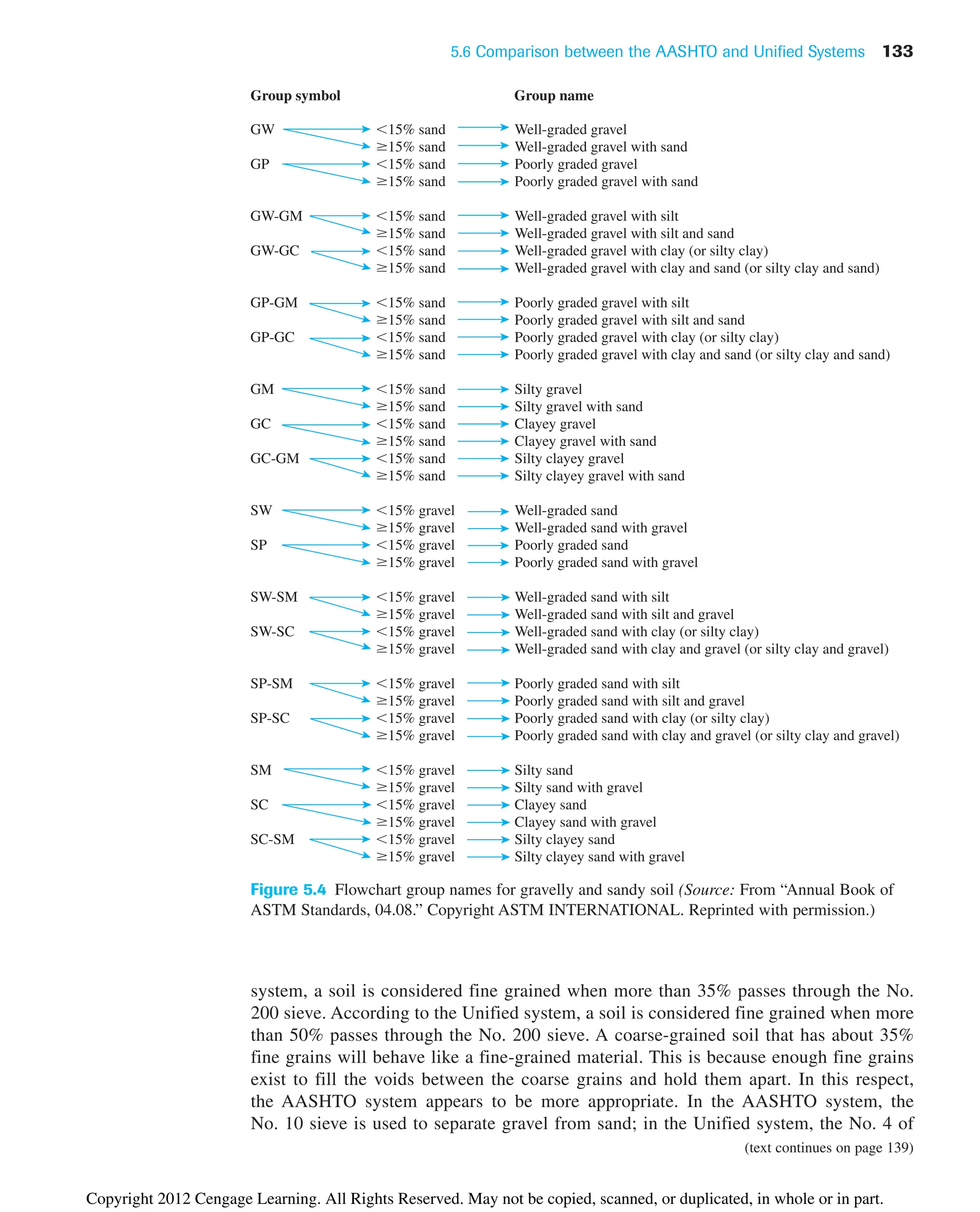
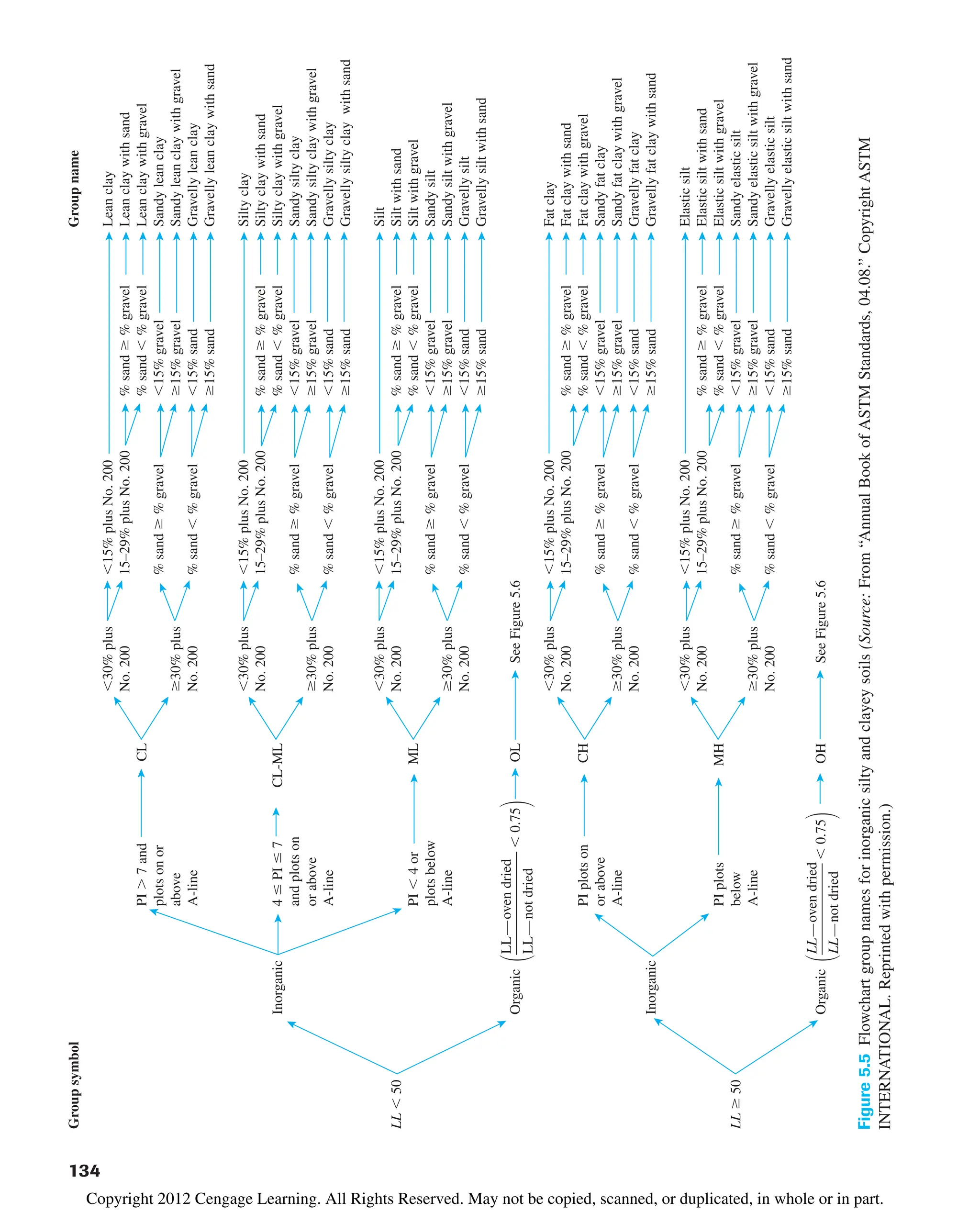
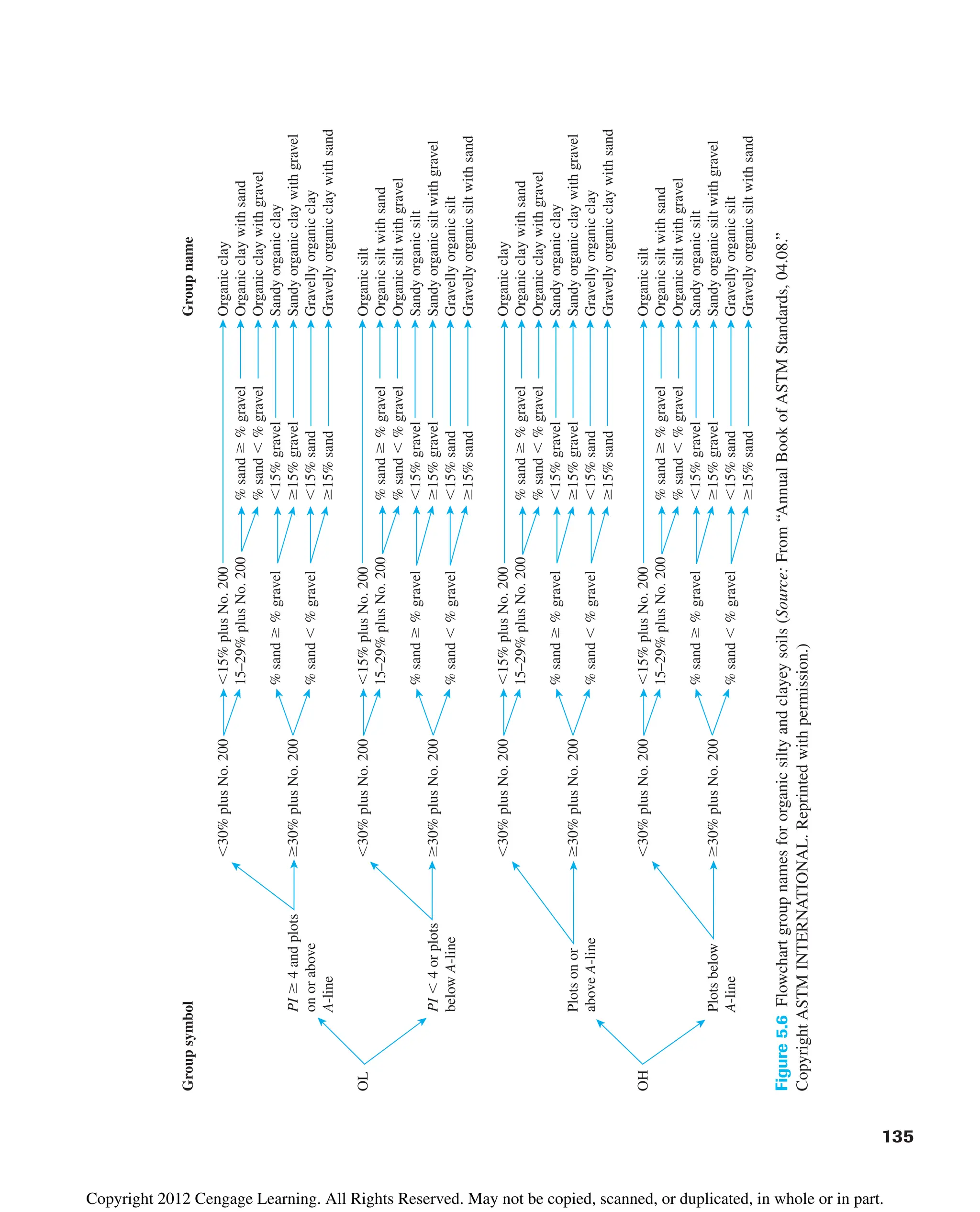
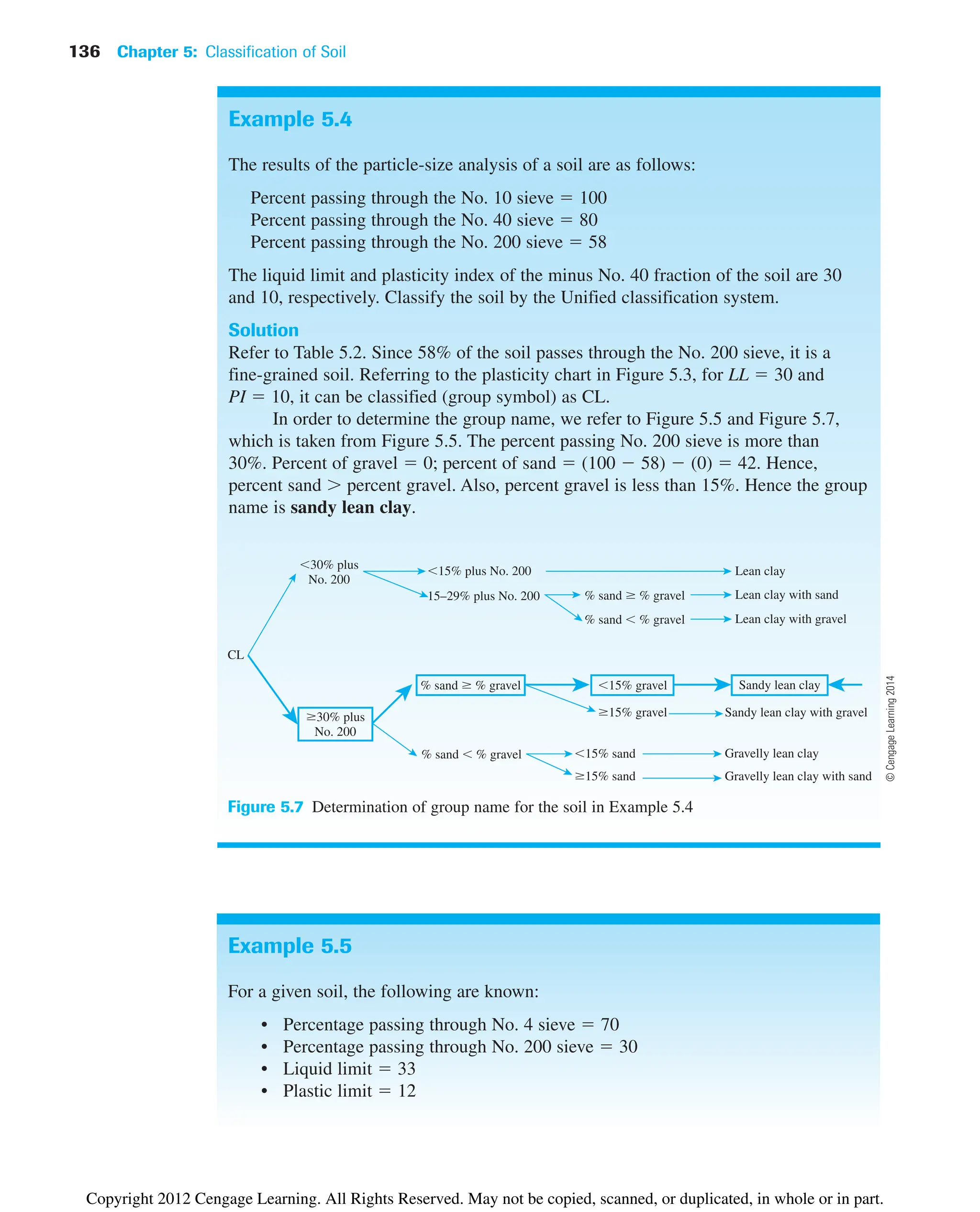
4. In addition to group symbols, the group names under the Unified classification sys-
tem can be determined using Figures 5.4, 5.5, and 5.6. The group name is primarily
based on percent retained on No. 200 sieve, percent of gravel (i.e., percent retained
on No. 4 sieve), and percent of sand (i.e., percent passing No. 4 sieve but retained
on No. 200 sieve).
5.1 Classify the following soil using the U.S. Department of Agriculture textural classi-
fication chart.
Particle-size
distribution (%)
Soil Sand Silt Clay
A 20 20 60
B 55 5 40
C 45 35 20
D 50 15 35
E 70 15 15
Problems
©
Cengage
Learning
2014
Copyright 2012 Cengage Learning. All Rights Reserved. May not be copied, scanned, or duplicated, in whole or in part.](https://image.slidesharecdn.com/principlesofgeotechnicalengineering-8thedition-231222125509-7e44d9bf/75/Principles-of-Geotechnical-Engineering-8th-Edition-pdf-162-2048.jpg)
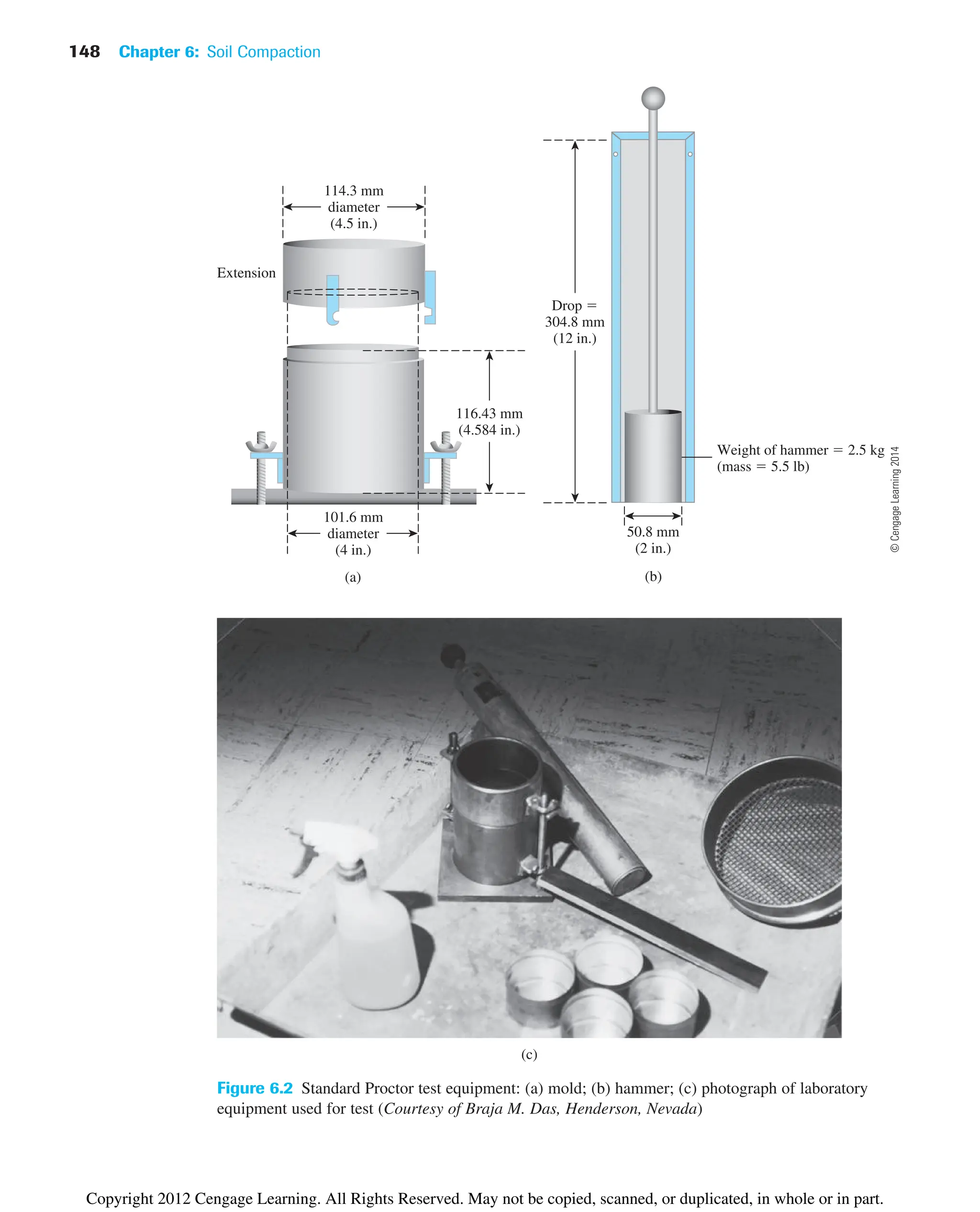
![150 Chapter 6: Soil Compaction
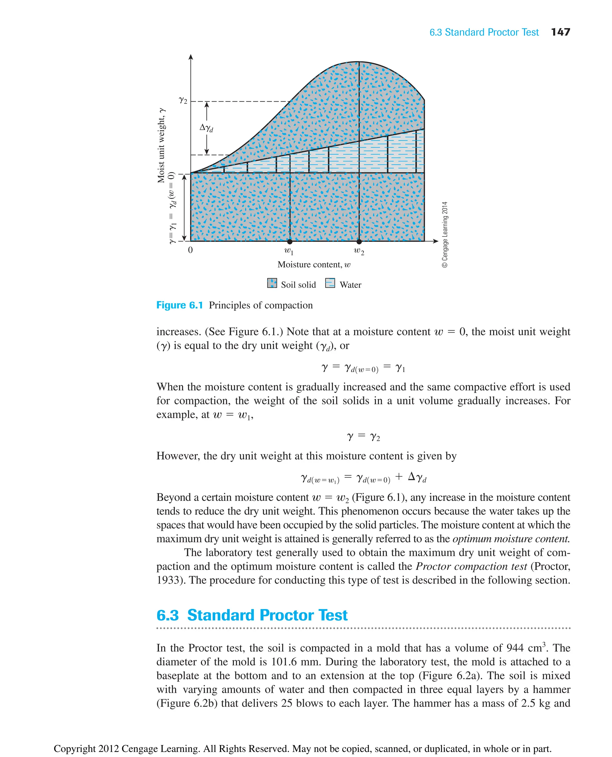
For a given moisture content w and degree of saturation S, the dry unit weight of
compaction can be calculated as follows. From Chapter 3 [Eq. (3.17)], for any soil,
where Gs ⫽ specific gravity of soil solids
gw ⫽ unit weight of water
e ⫽ void ratio
and, from Eq. (3.19),
or
Thus,
(6.3)
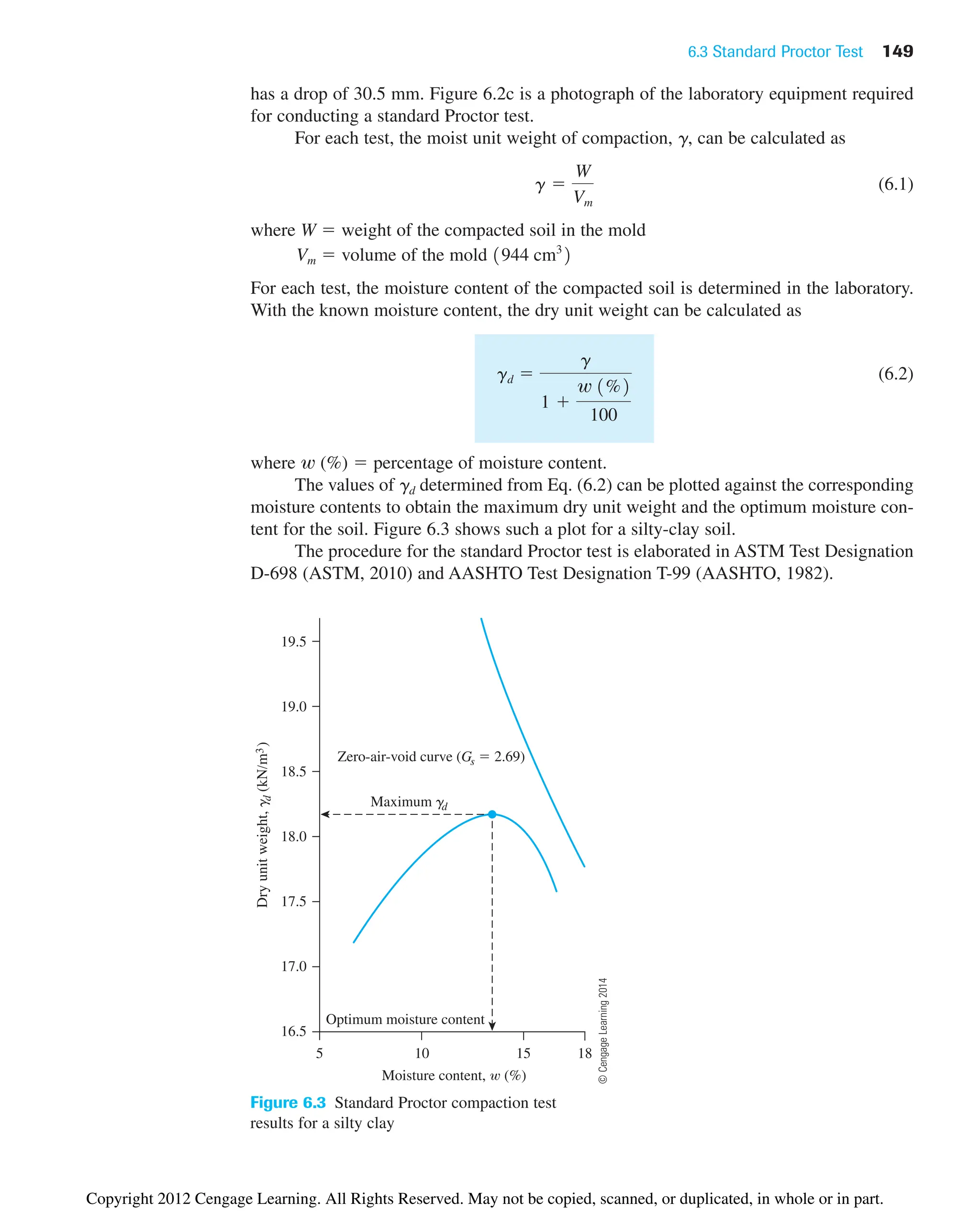
For a given moisture content, the theoretical maximum dry unit weight is obtained
when no air is in the void spaces—that is, when the degree of saturation equals 100%.
Hence, the maximum dry unit weight at a given moisture content with zero air voids can
be obtained by substituting S ⫽ 1 into Eq. (6.3), or
(6.4)
where gzav ⫽ zero-air-void unit weight.
To obtain the variation of gzav with moisture content, use the following procedure:
1. Determine the specific gravity of soil solids.
2. Know the unit weight of water (gw).
3. Assume several values of w, such as 5%, 10%, 15%, and so on.
4. Use Eq. (6.4) to calculate gzav for various values of w.
Figure 6.3 also shows the variation of gzav with moisture content and its relative loca-
tion with respect to the compaction curve. Under no circumstances should any part of the
compaction curve lie to the right of the zero-air-void curve.
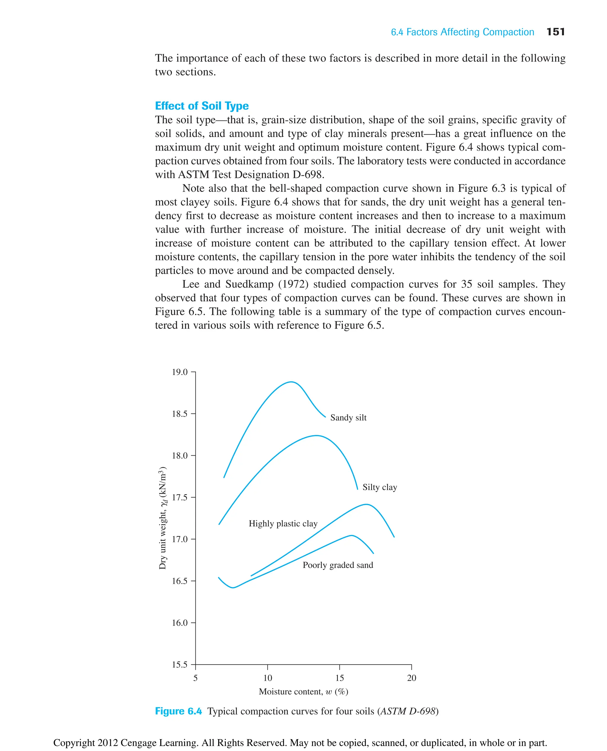
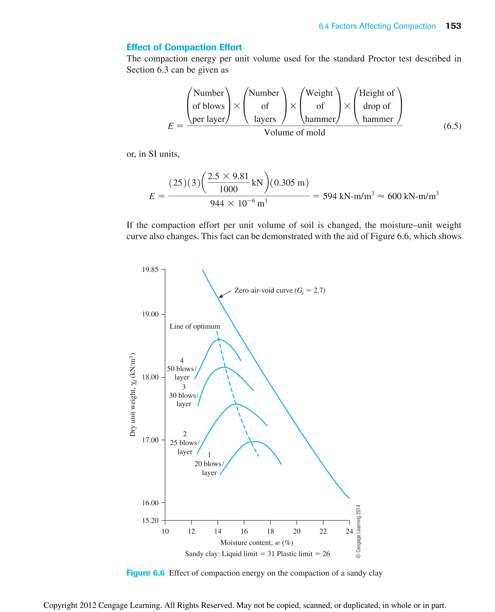
6.4 Factors Affecting Compaction
The preceding section showed that moisture content has a strong influence on the degree
of compaction achieved by a given soil. Besides moisture content, other important fac-
tors that affect compaction are soil type and compaction effort (energy per unit volume).
gzav ⫽
Gsgw
1 ⫹ wGs
⫽
gw
w ⫹
1
Gs
gd ⫽
Gsgw
1 ⫹
Gsw
S
e ⫽
Gsw
S
Se ⫽ Gsw
gd ⫽
GSgw
1 ⫹ e
Copyright 2012 Cengage Learning. All Rights Reserved. May not be copied, scanned, or duplicated, in whole or in part.](https://image.slidesharecdn.com/principlesofgeotechnicalengineering-8thedition-231222125509-7e44d9bf/75/Principles-of-Geotechnical-Engineering-8th-Edition-pdf-170-2048.jpg)
![6.6 Empirical Relationships 157
Gurtug and Sridharan (2004) proposed correlations for optimum moisture content
and maximum dry unit weight with the plastic limit (PL) of cohesive soils. These correla-
tions can be expressed as:
(6.11)
(6.12)
where PL ⫽ plastic limit (%)
E ⫽ compaction energy (kN-m/m3
)
For modified Proctor test, E 2700 kN/m3
. Hence,
and
Osman et al. (2008) analyzed a number of laboratory compaction test results on fine-
grained (cohesive) soil, including those provided by Gurtug and Sridharan (2004). Based
on this study, the following correlations were developed:
(6.13)
and
(6.14)
where
(6.15)
(6.16)
wopt ⫽ optimum water content (%)
PI ⫽ plasticity index (%)
gd(max) ⫽ maximum dry unit weight (kN/m3
)
E ⫽ compaction energy (kN-m/m3
)
Matteo et al. (2009) analyzed the results of 71 fine-grained soils and provided the
following correlations for optimum water content (wopt) and maximum dry unit weight
[gd(max)] for modified Proctor tests (E ⫽ 2700 kN-m/m3
):
(6.17)
and
(6.18)
where LL ⫽ liquid limit (%)
PI ⫽ plasticity index (%)
Gs ⫽ specific gravity of soil solids
gd1max21kN/m3
2 ⫽ 40.3161wopt
⫺0.295
21PI0.032
2 ⫺ 2.4
wopt1%2 ⫽ ⫺0.861LL2 ⫹ 3.04a
LL
Gs
b ⫹ 2.2
M ⫽ ⫺0.19 ⫹ 0.073 ln E
L ⫽ 14.34 ⫹ 1.195 ln E
gd1max2 1kN/m3
2 ⫽ L ⫺ Mwopt
wopt1%2 ⫽ 11.99 ⫺ 0.165 ln E21PI2
gd1max2 1kN/m3
2 ⫽ 22.68e⫺0.0121PL2
wopt1%2 ⬇ 0.65 1PL2
⫽
gd1max2 1kN/m3
2 ⫽ 22.68e⫺0.0183wopt1%2
wopt1%2 ⫽ 31.95 ⫺ 0.381log E241PL2
Copyright 2012 Cengage Learning. All Rights Reserved. May not be copied, scanned, or duplicated, in whole or in part.](https://image.slidesharecdn.com/principlesofgeotechnicalengineering-8thedition-231222125509-7e44d9bf/75/Principles-of-Geotechnical-Engineering-8th-Edition-pdf-177-2048.jpg)
![6.15 Summary and General Comments
In this chapter, we have discussed the following:
• Standard and modified Proctor compaction tests are conducted in the laboratory to
determine the maximum dry unit weight of compaction [gd(max)] and optimum mois-
ture content (wopt) (Sections 6.3 and 6.5).
• gd(max) and wopt are functions of the energy of compaction E.
• Several empirical relations have been presented to estimate gd(max) and wopt for
cohesionless and cohesive soils (Section 6.6). Also included in this section is an
empirical relationship to estimate the relative density of compaction (Dr) with known
median grain size (D50) and energy of compaction (E).
• For a given energy of compaction (E) in a cohesive soil, the hydraulic conductivity
and unconfined compression strength, swelling, and shrinkage characteristics are
functions of molding moisture content.
• Field compaction is generally carried out by rollers such as smooth-wheel, rubber-
tired, sheepsfoot, and vibratory (Section 6.9).
• Control tests to determine the quality of field compaction can be done by using the
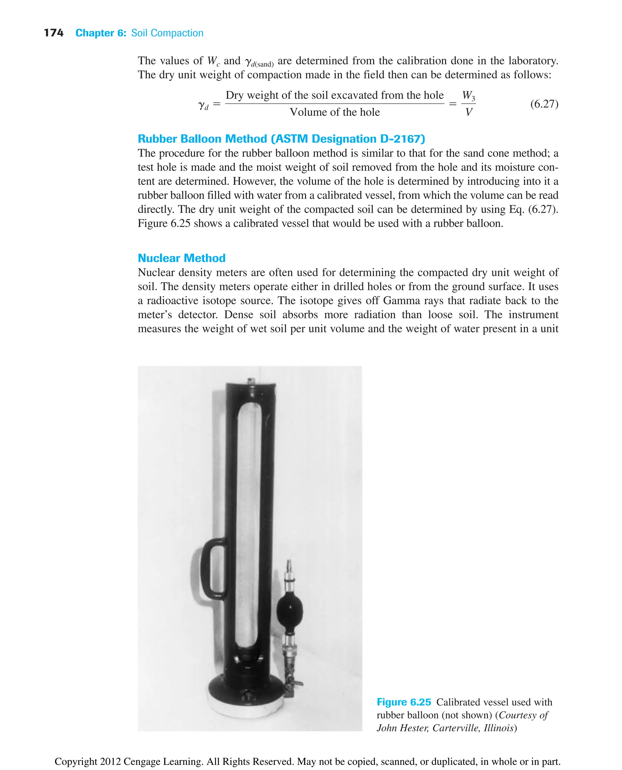
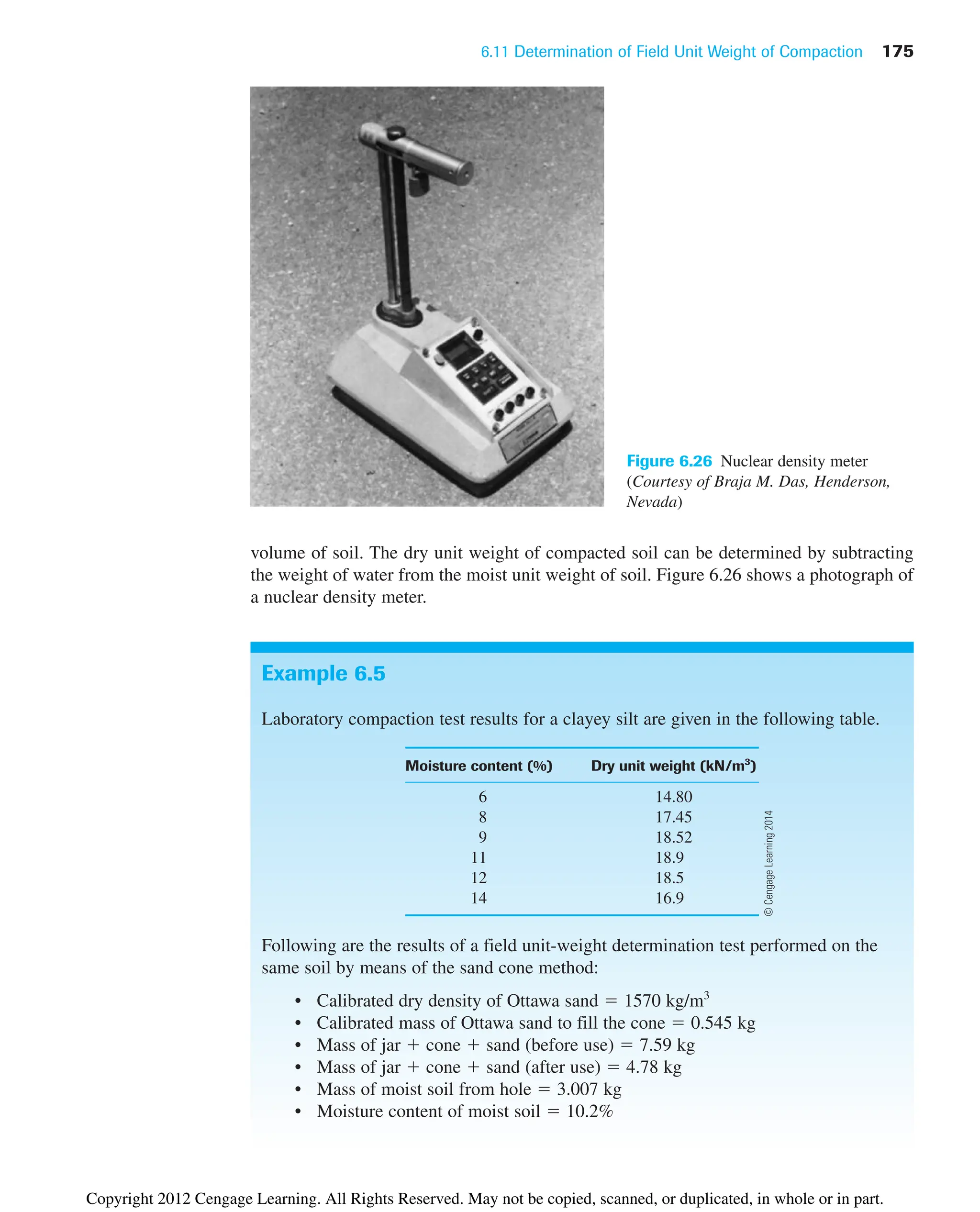
sand cone method, rubber balloon method, and nuclear method.
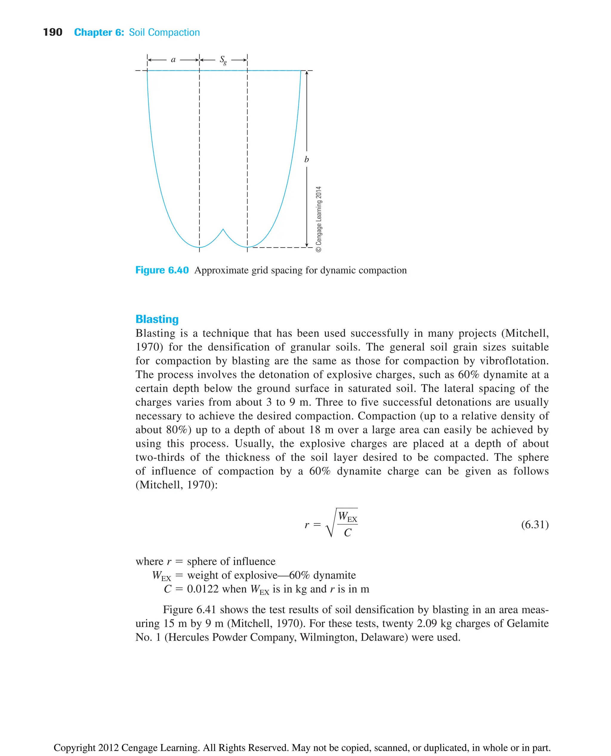
• Vibroflotation, dynamic compaction, and blasting are special techniques used for
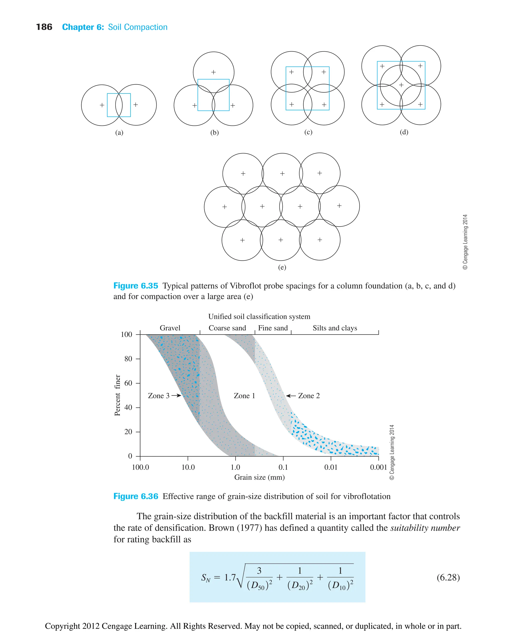
large-scale compaction in the field (Section 6.14).
Laboratory standard and modified Proctor compaction tests described in this chapter are
essentially for impact or dynamic compaction of soil; however, in the laboratory, static
compaction and kneading compaction also can be used. It is important to realize that the
compaction of clayey soils achieved by rollers in the field is essentially the kneading
type. The relationships of dry unit weight (gd) and moisture content (w) obtained by
dynamic and kneading compaction are not the same. Proctor compaction test results
obtained in the laboratory are used primarily to determine whether the roller compaction
in the field is sufficient. The structures of compacted cohesive soil at a similar dry unit
weight obtained by dynamic and kneading compaction may be different. This difference,
in turn, affects physical properties, such as hydraulic conductivity, compressibility, and
strength.
For most fill operations, the final selection of the borrow site depends on such factors
as the soil type and the cost of excavation and hauling.
192 Chapter 6: Soil Compaction
Problems
6.1 Calculate and plot the variation of dry density of a soil in kg/m3
(Gs ⫽ 2.65)
at w ⫽ 5, 10, 15, and 20% for degree of saturation, S ⫽ 70, 80, 90, and 100%.
6.2 Calculate the zero-air-void unit weights (kN/m3
) for a soil with Gs ⫽ 2.68 at
moisture contents of 5, 10, 15, 20, and 25%.
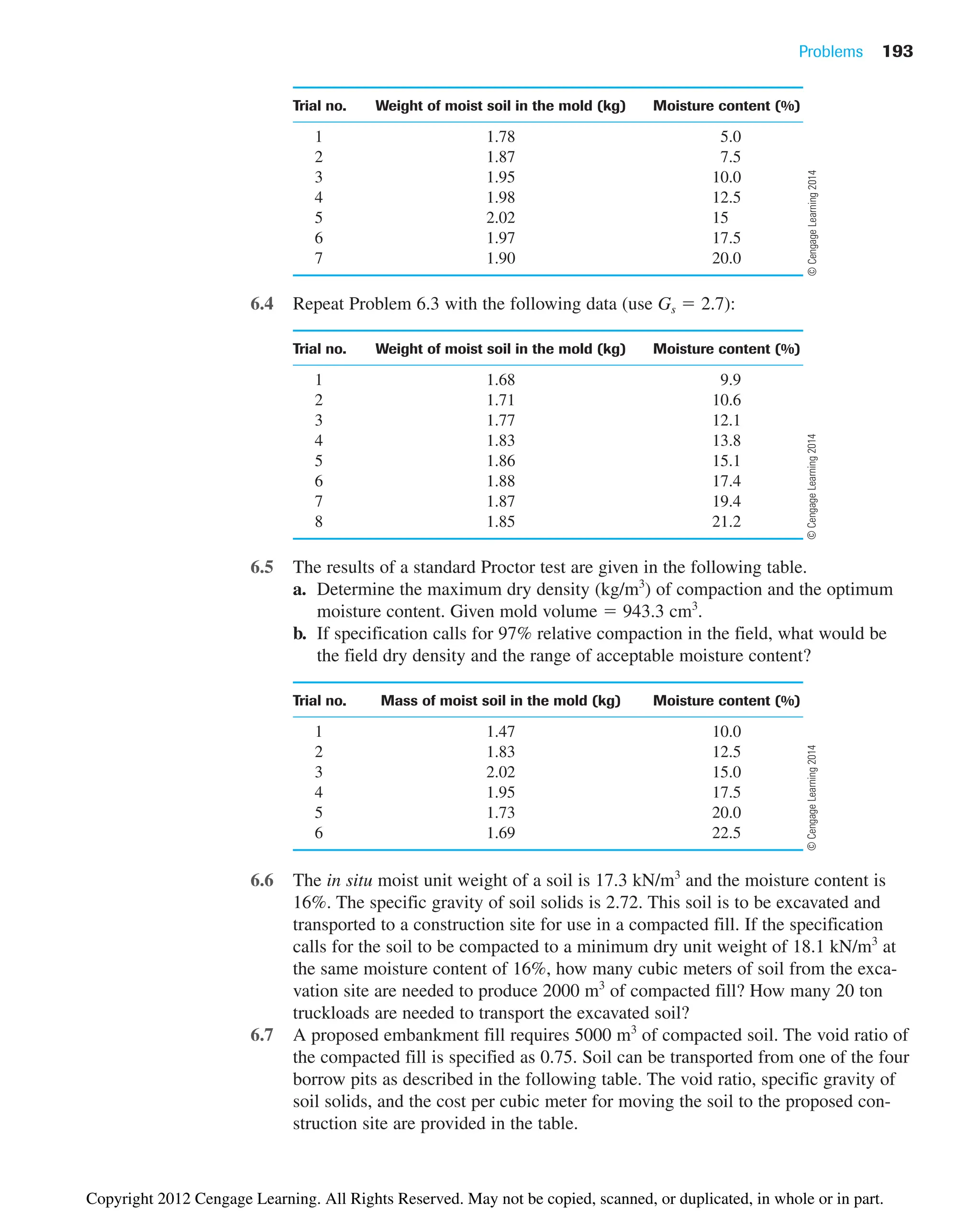
6.3 The results of a standard Proctor test are given in the following table.
a. Determine the maximum dry unit weight of compaction and the optimum
moisture content. Given: mold volume⫽943.3 cm3
.
b. Determine the void ratio and the degree of saturation at the optimum moisture
content. Given: Gs ⫽ 2.68.
Copyright 2012 Cengage Learning. All Rights Reserved. May not be copied, scanned, or duplicated, in whole or in part.](https://image.slidesharecdn.com/principlesofgeotechnicalengineering-8thedition-231222125509-7e44d9bf/75/Principles-of-Geotechnical-Engineering-8th-Edition-pdf-212-2048.jpg)
![References 195
optimum moisture content and maximum dry unit weight. Let us use some of
these equations and compare our results with known experimental data.
The following table presents the results from laboratory compaction tests con-
ducted on a wide range of fine-grained soils using various compactive efforts (E).
Based on the soil data given in the table, determine the optimum moisture content and
maximum dry unit weight using the empirical relationships presented in Section 6.6.
a. Use the Osman et al. (2008) method [Eqs. (6.13) through (6.16)].
b. Use the Gurtug and Sridharan (2004) method [Eqs. (6.11) and (6.12)].
c. Use the Matteo et al. (2009) method [Eqs. (6.17) and (6.18)].
d. Plot the calculated wopt against the experimental wopt, and the calculated gd(max)
with the experimental gd(max). Draw a 45° line of equality on each plot.
e. Comment on the predictive capabilities of various methods. What can you say
about the inherent nature of empirical models?
Soil Gs LL (%) PL (%) E (kN-m/m3
) wopt (%) gd(max) (kN/m3
)
1a
2.67 17 16 2700b
8 20.72
600c
10 19.62
354d
10 19.29
2a
2.73 68 21 2700 20 16.00
600 28 13.80
354 31 13.02
3 2.68 56 14 2700 15 18.25
1300e
16 17.5
600 17 16.5
275f
19 15.75
4 2.68 66 27 600 21 15.89
5 2.67 25 21 600 18 16.18
6 2.71 35 22 600 17 16.87
7 2.69 23 18 600 12 18.63
8 2.72 29 19 600 15 17.65
Note:
a
Tschebotarioff (1951)
b
Modified Proctor test
c
Standard Proctor test
d
Standard Proctor mold and hammer; drop: 305 mm; layers: 3; blows/layer: 15
e
Modified Proctor mold and hammer; drop: 457 mm; layers: 5; blows/layer: 26
f
Modified Proctor mold; standard Proctor hammer; drop: 305 mm; layers: 3; blows/layer: 25
References
AMERICAN ASSOCIATION OF STATE HIGHWAY AND TRANSPORTATION OFFICIALS (1982). AASHTO
Materials, Part II, Washington, D.C.
AMERICAN SOCIETY FOR TESTING AND MATERIALS (2010). Annual Book of ASTM Standards,
Vol 04.08, West Conshohocken, Pa.
BROWN, E. (1977). “Vibroflotation Compaction of Cohesionless Soils,” Journal of the Geo technical
Engineering Division, ASCE, Vol. 103, No. GT12, 1437–1451.
D’APPOLONIA, D. J., WHITMAN, R. V., and D’APPOLONIA, E. D. (1969). “Sand Compaction with
Vibratory Rollers,” Journal of the Soil Mechanics and Foundations Division, ASCE, Vol. 95,
No. SM1, 263–284.
©
Cengage
Learning
2014
Copyright 2012 Cengage Learning. All Rights Reserved. May not be copied, scanned, or duplicated, in whole or in part.](https://image.slidesharecdn.com/principlesofgeotechnicalengineering-8thedition-231222125509-7e44d9bf/75/Principles-of-Geotechnical-Engineering-8th-Edition-pdf-215-2048.jpg)
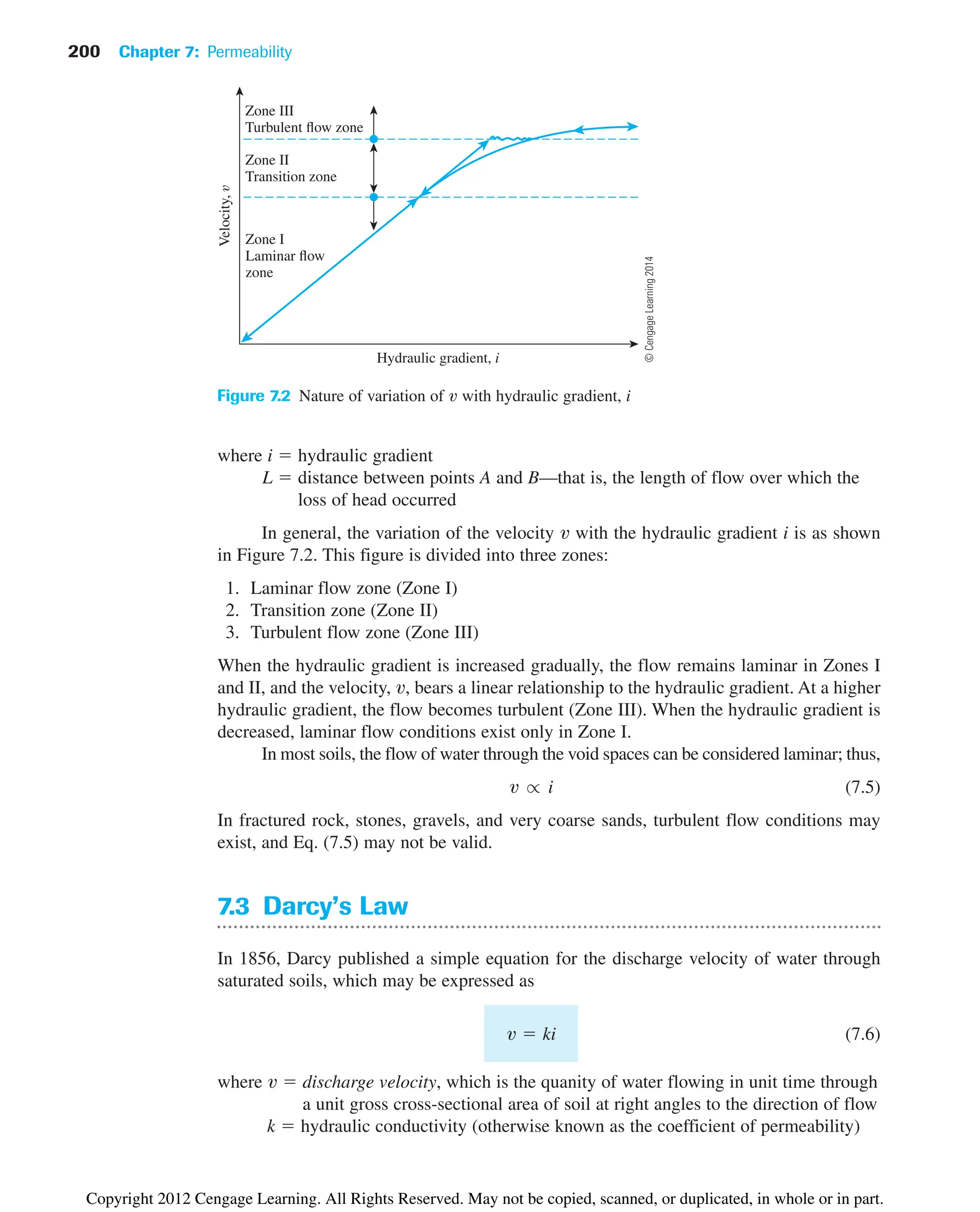
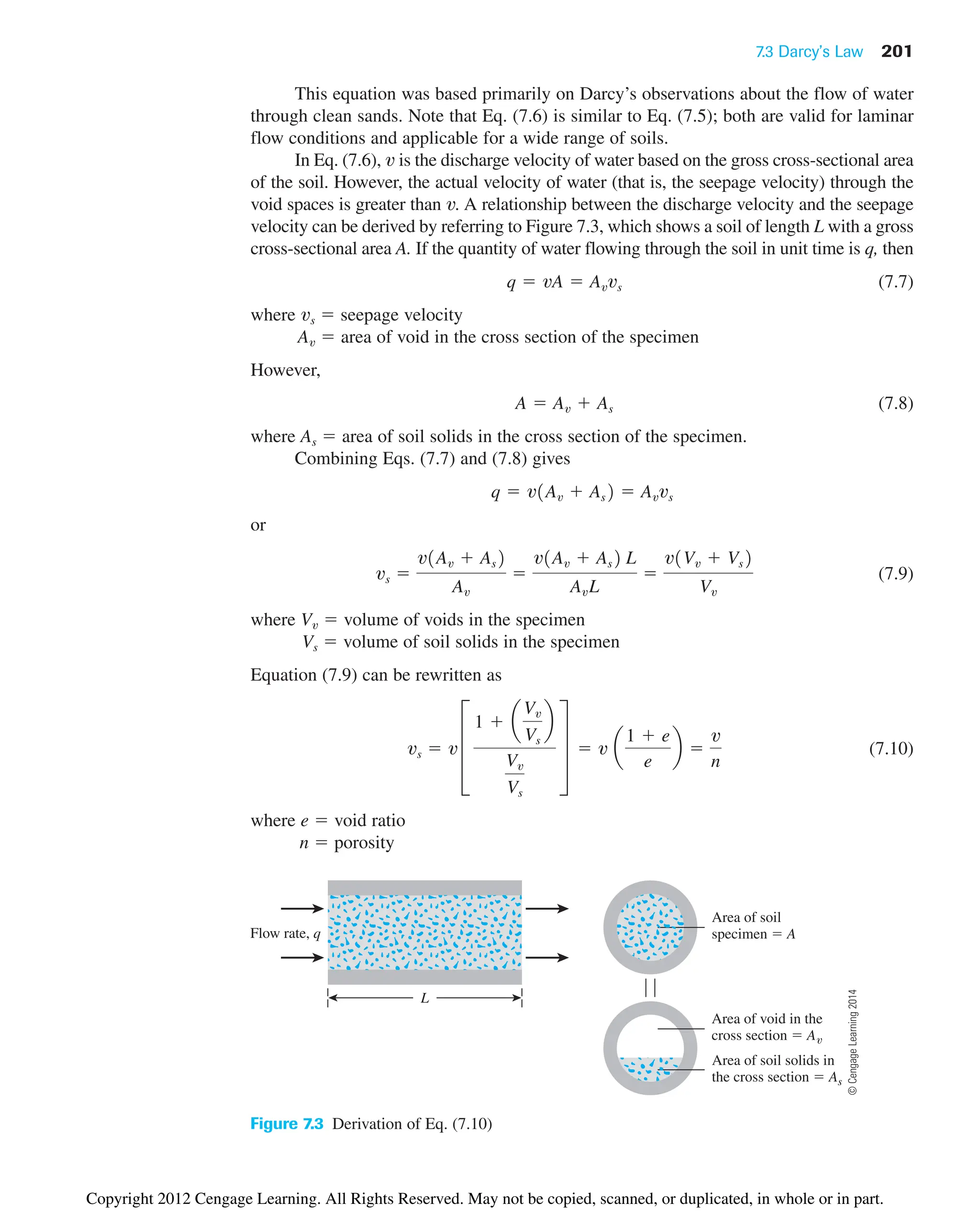
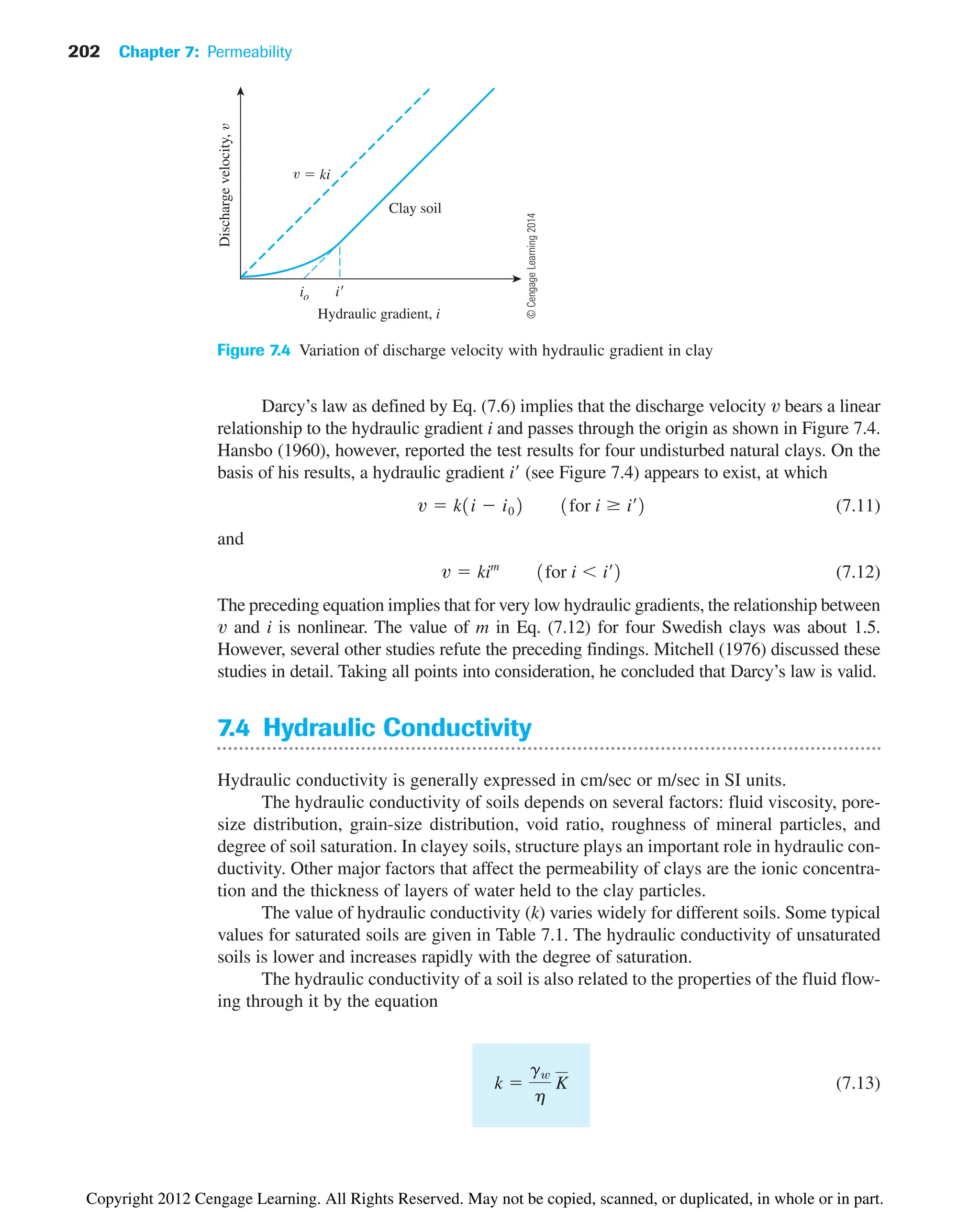
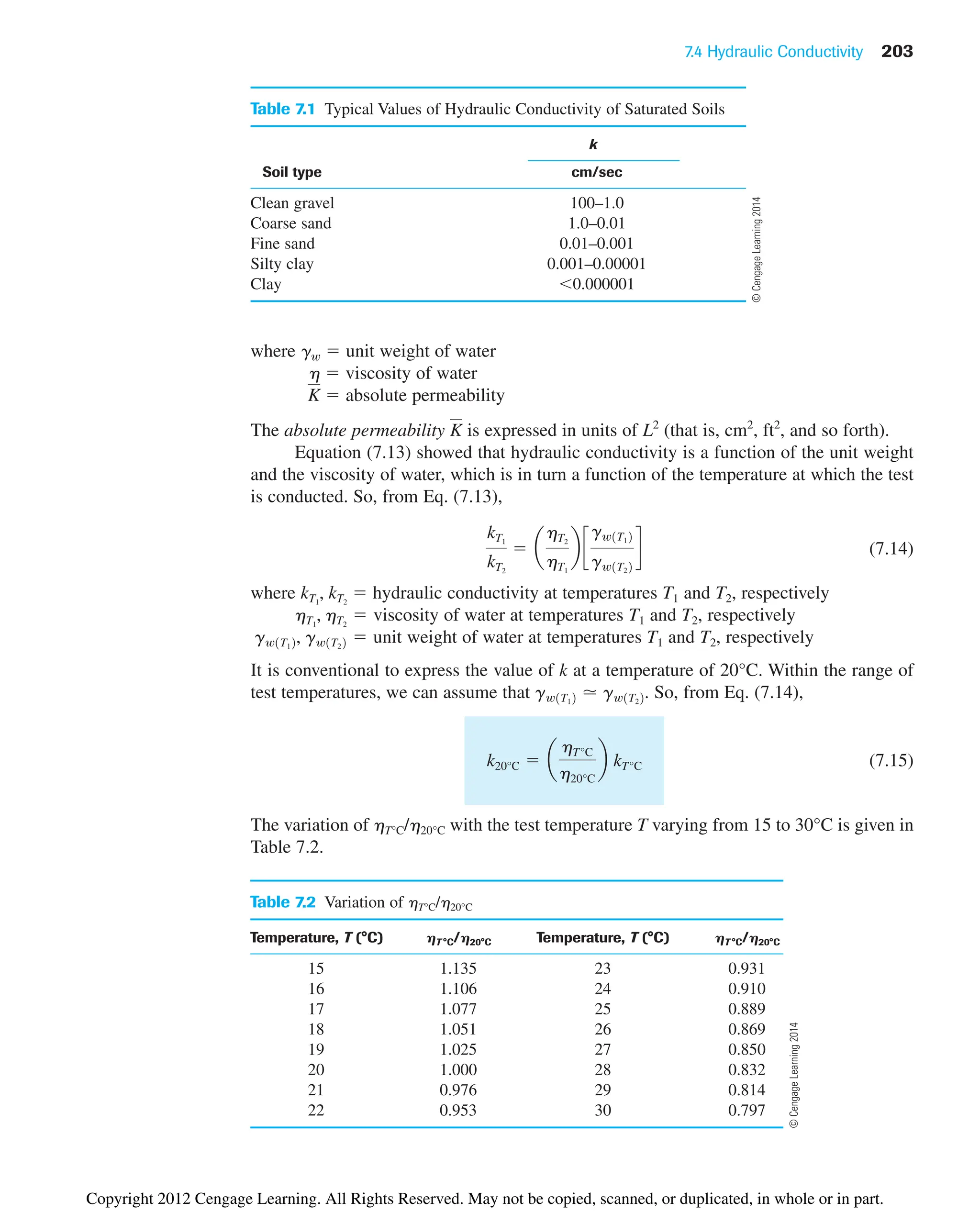
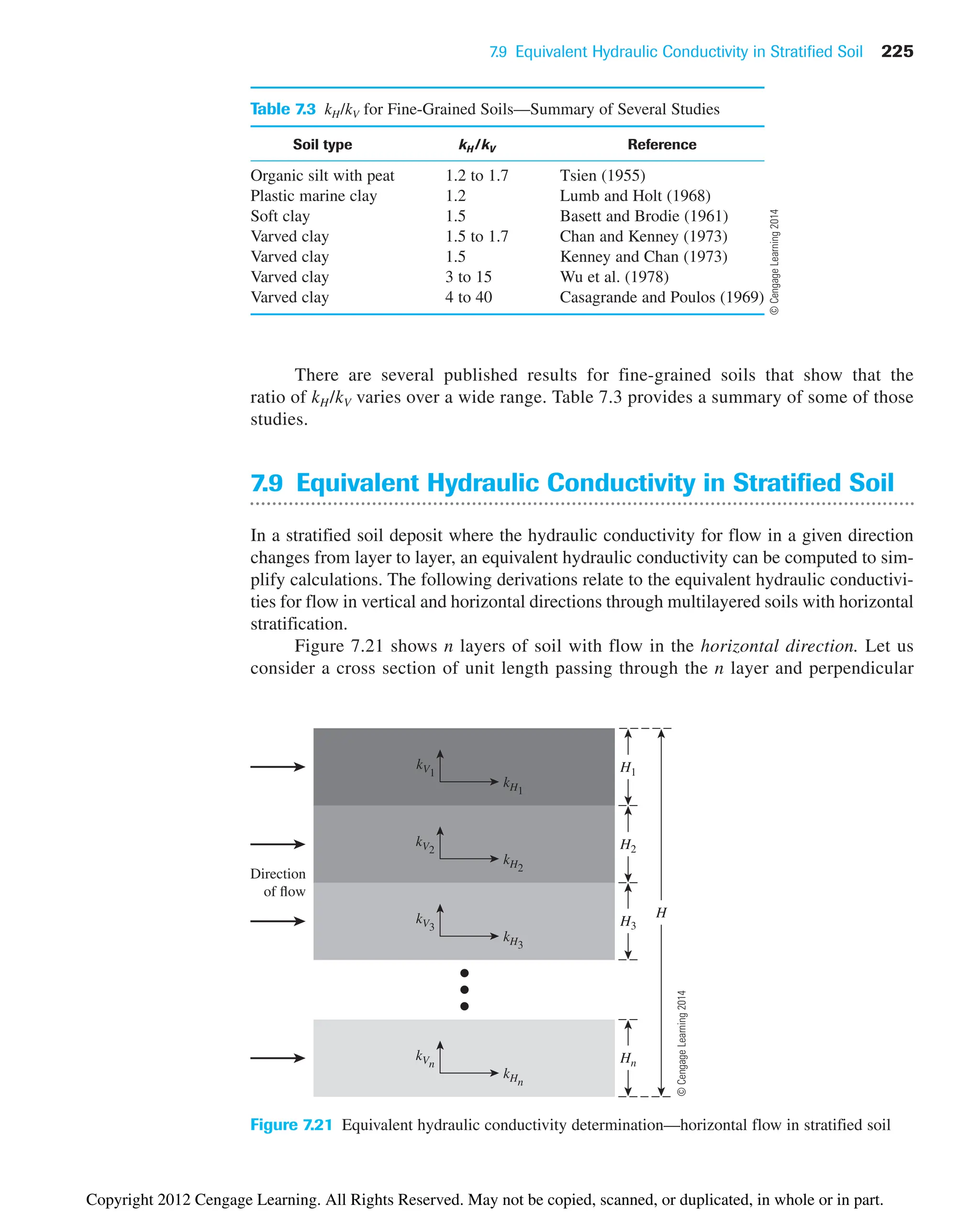
![218 Chapter 7: Permeability
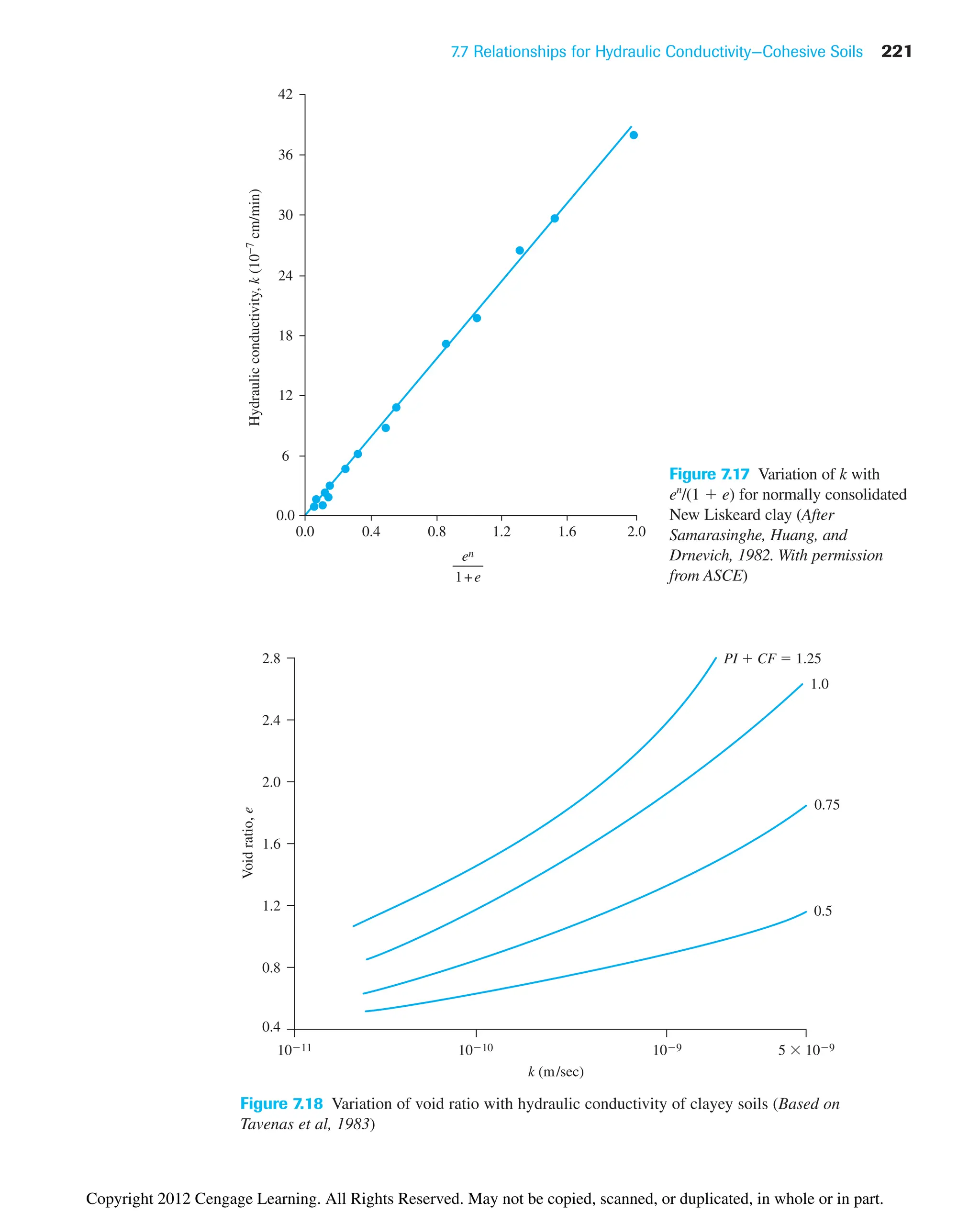
7.7 Relationships for Hydraulic
Conductivity—Cohesive Soils
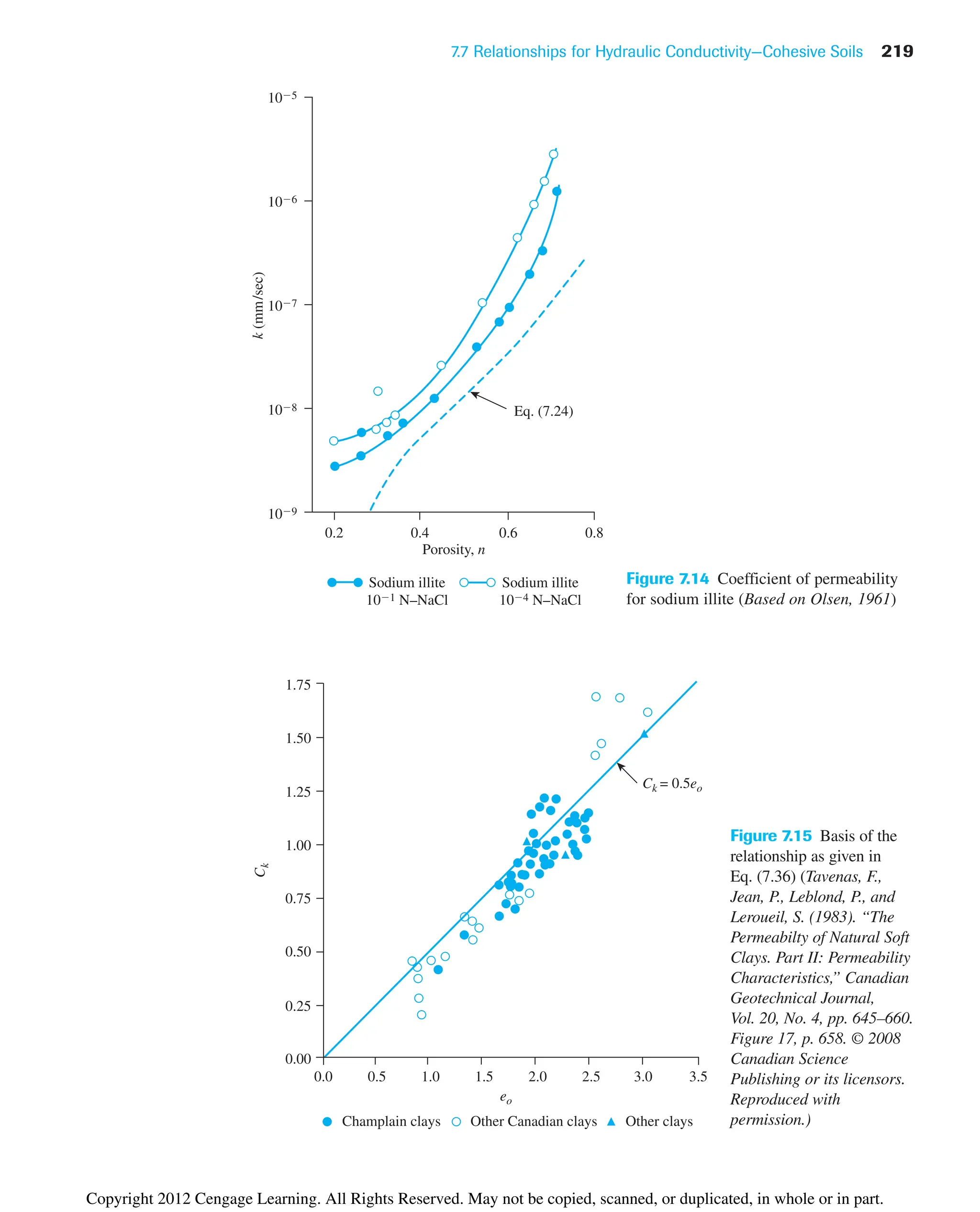
The Kozeny–Carman equation [Eq. (7.24)] has been used in the past to see if it will hold
good for cohesive soil. Olsen (1961) conducted hydraulic conductivity tests on sodium
illite and compared the results with Eq. (7.24). This comparison is shown in Figure 7.14.
The marked degrees of variation between the theoretical and experimental values arise
from several factors, including deviations from Darcy’s law, high viscosity of the pore
water, and unequal pore sizes.
Taylor (1948) proposed a linear relationship between the logarithm of k and the void
ratio as
(7.36)
where ko in situ hydraulic conductivity at a void ratio eo
k hydraulic conductivity at a void ratio e
Ck hydraulic conductivity change index
The preceding equation is a good correlation for eo less than about 2.5. In this equation,
the value of Ck may be taken to be about 0.5eo (see Figure 7.15).
For a wide range of void ratio, Mesri and Olson (1971) suggested the use of a linear
relationship between log k and log e in the form
(7.37)
log k A¿ log e B¿
log k log ko
eo e
Ck
Example 7.9
Solve Example 7.7 using Eq. (7.34).
Solution
From Figure 7.13, D60 0.16 mm and D10 0.09 mm. Thus,
From Eq. (7.34),
k 35a
e3
1 e
bCu
0.6
1D1022.32
35a
0.63
1 0.6
b11.7820.6
10.0922.32
0.025 cm/sec
Cu
D60
D10
0.16
0.09
1.78
Copyright 2012 Cengage Learning. All Rights Reserved. May not be copied, scanned, or duplicated, in whole or in part.](https://image.slidesharecdn.com/principlesofgeotechnicalengineering-8thedition-231222125509-7e44d9bf/75/Principles-of-Geotechnical-Engineering-8th-Edition-pdf-238-2048.jpg)
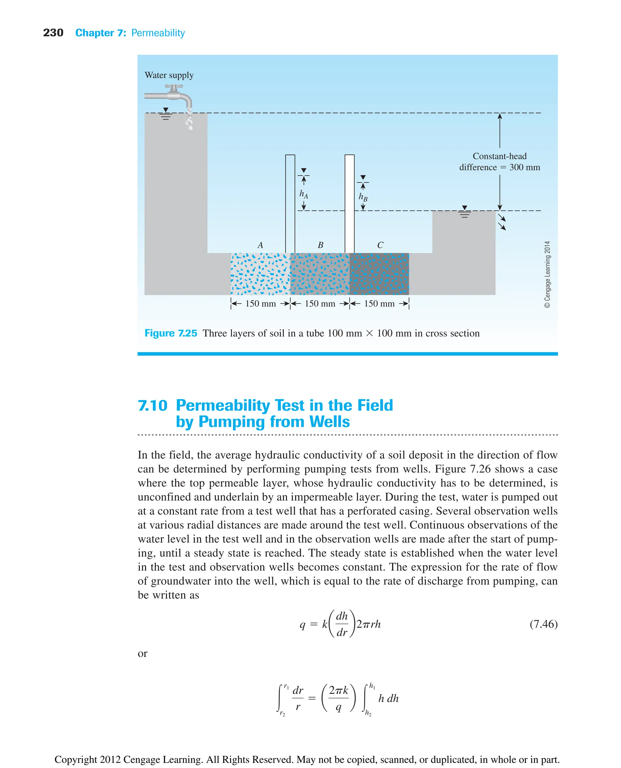
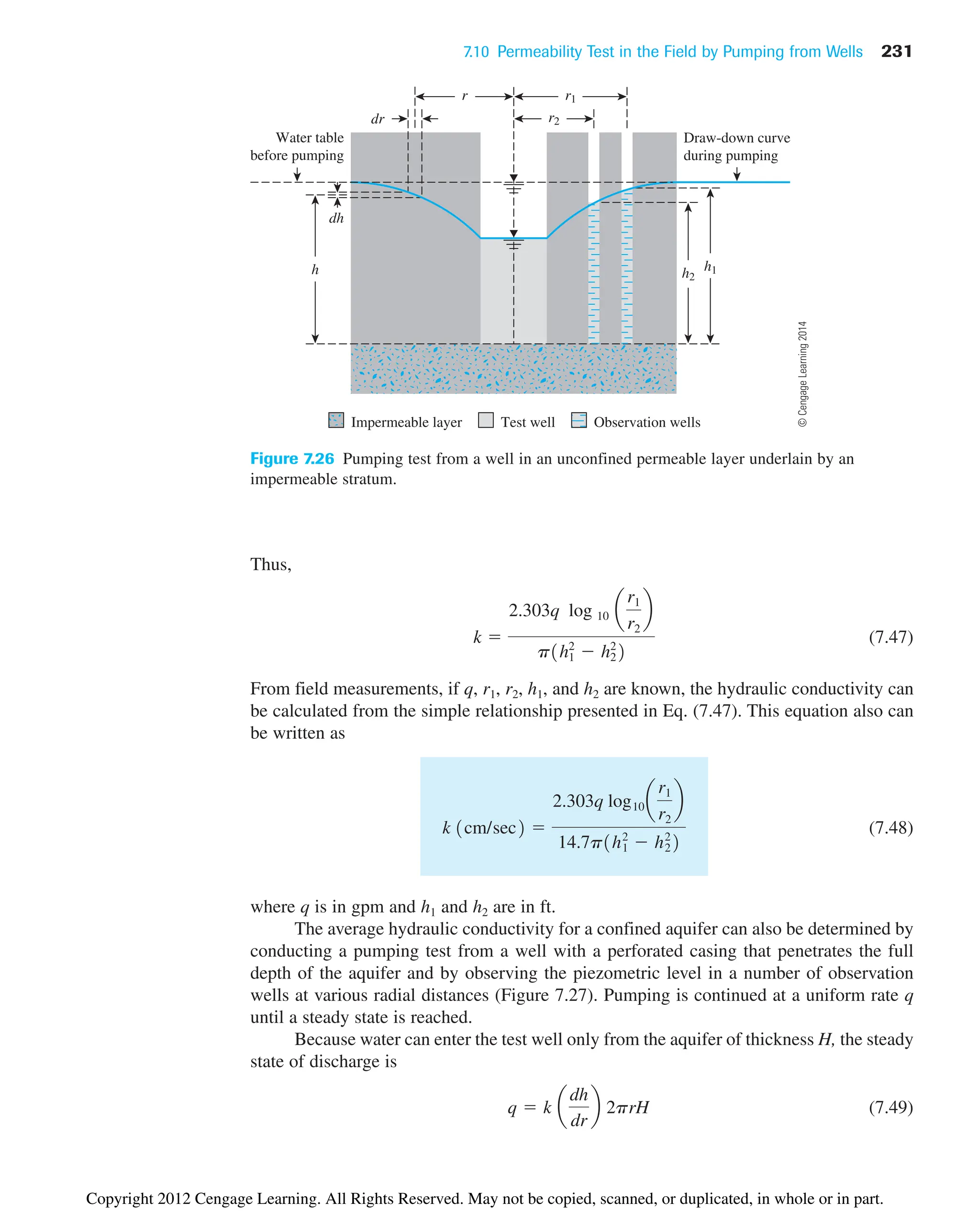
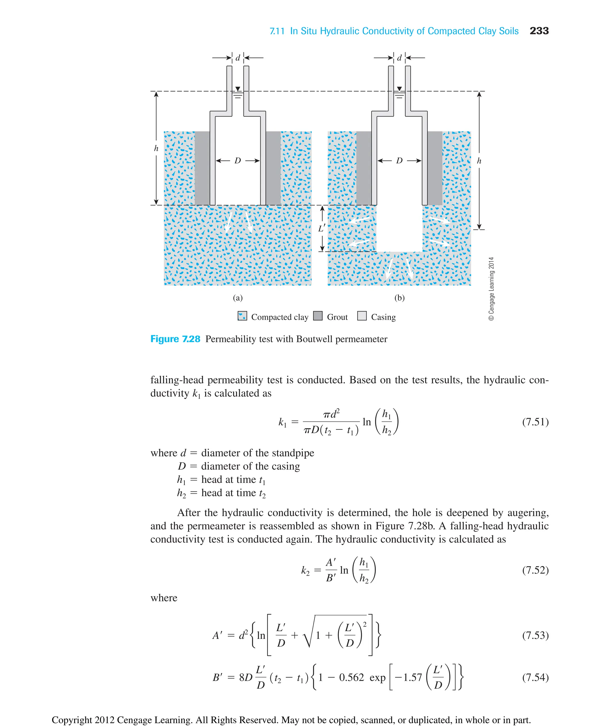
![234 Chapter 7: Permeability
The anisotropy with respect to hydraulic conductivity is determined by referring to
Figure 7.29, which is a plot of k2/k1 versus for various values of L/D.
Figure 7.29 can be used to determine m using the experimental values of k2/k1 and L9/D.
The plots in this figure are determined from
(7.55)
Once m is determined, we can calculate
(7.56)
and
(7.57)
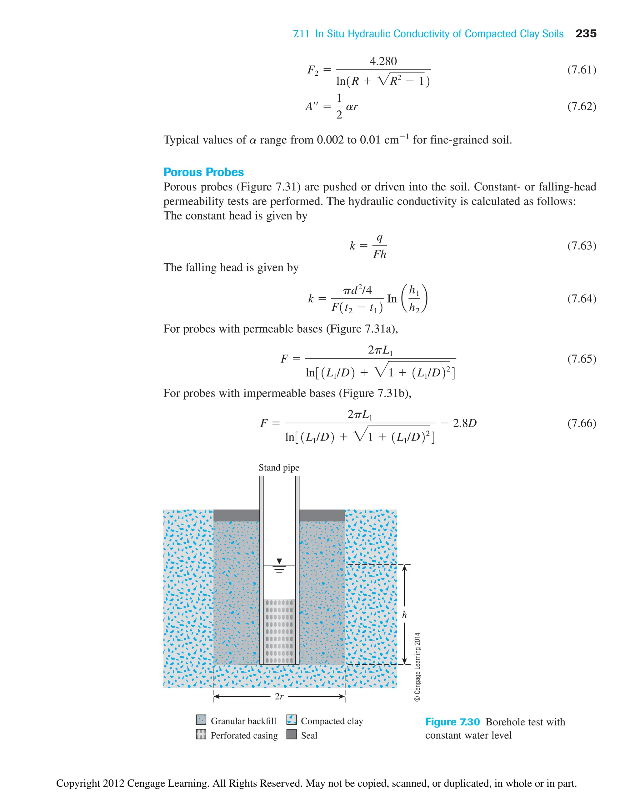
Constant-Head Borehole Permeameter
Figure 7.30 shows a constant-head borehole permeameter. In this arrangement a constant
head h is maintained by supplying water, and the rate of flow q is measured. The hydraulic
conductivity can be calculated as
(7.58)
where
(7.59)
(7.60)
F1
4.11711 R2
2
ln1R 2R2
12 31 11/R2
240.5
R
h
r
k
q
r2
2R2
13F1 1F2/Aœœ
24
kV
k1
m
kH mk1
k2
k1
ln31L¿/D2 31 1L¿/D22
4
ln31mL¿/D2 31 1mL¿/D22
4
m
m 1m 3kH/kV2
1
0
4
8
12
2
1.5
L D 1.0
2.0
3 4
k2/k1
m
Figure 7.29
Variation of k2/k1 with m [Eq. (7.55)]
©
Cengage
Learning
2014
Copyright 2012 Cengage Learning. All Rights Reserved. May not be copied, scanned, or duplicated, in whole or in part.](https://image.slidesharecdn.com/principlesofgeotechnicalengineering-8thedition-231222125509-7e44d9bf/75/Principles-of-Geotechnical-Engineering-8th-Edition-pdf-254-2048.jpg)
![236 Chapter 7: Permeability
7.12 Summary and General Comments
Following is a summary of the important subjects covered in this chapter.
• Darcy’s law can be expressed as
discharge hydraulic hydraulic
velocity conductivity gradient
• Seepage velocity (vs) of water through the void spaces can be given as
• Hydraulic conductivity is a function of viscosity (and hence temperature) of water.
• Constant-head and falling-head types of tests are conducted to determine the
hydraulic conductivity of soils in the laboratory (Section 7.5).
• There are several empirical correlations for hydraulic conductivity in granular and
cohesive soil. Some of those are given in Sections 7.6 and 7.7. It is important, how-
ever, to realize that these are only approximations, since hydraulic conductivity is a
highly variable quantity.
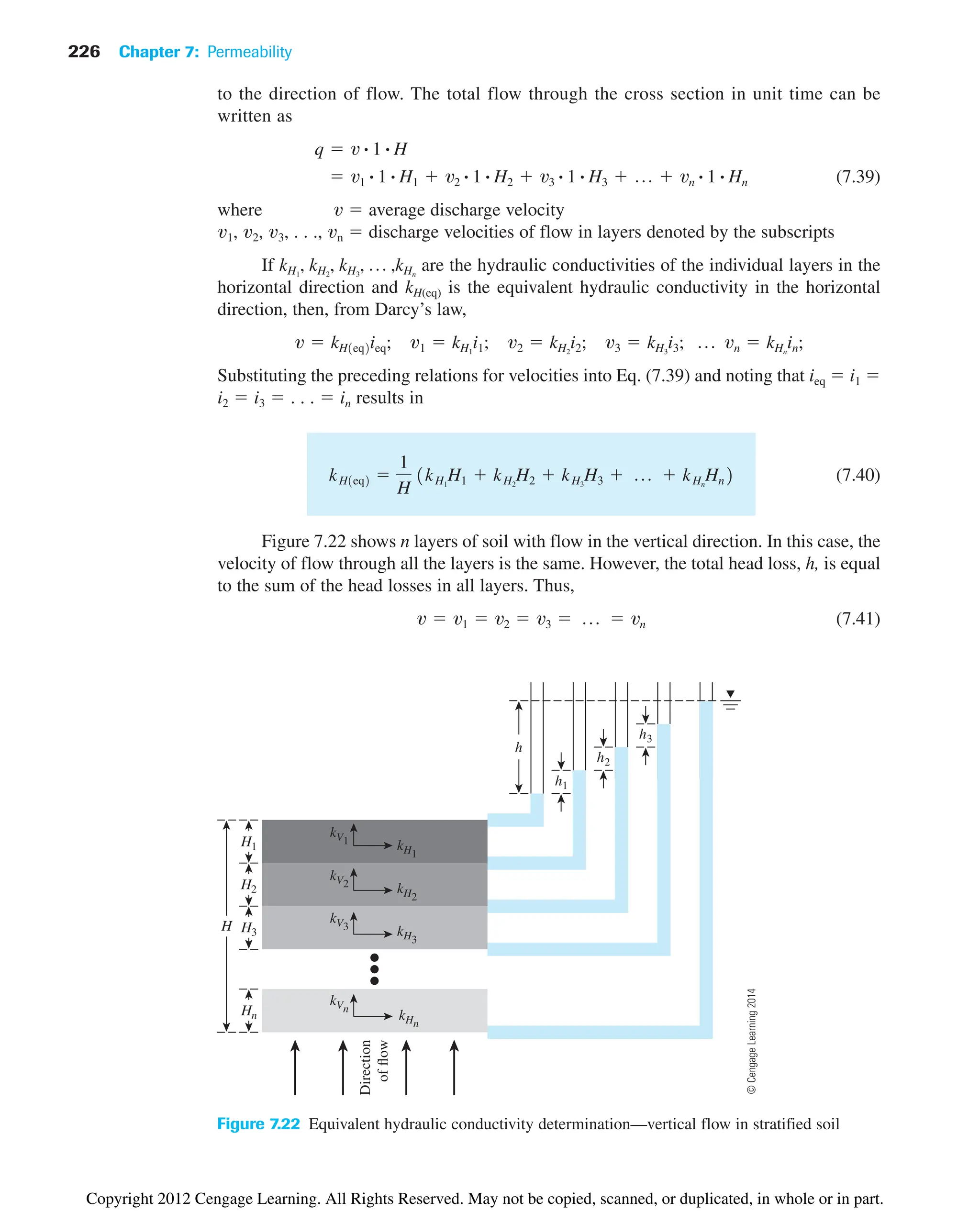
• For layered soil, depending on the direction of flow, an equivalent hydraulic con-
ductivity relation can be developed to estimate the quantity of flow [Eqs. (7.40)
and (7.45)].
• Hydraulic conductivity in the field can be determined by pumping from wells
(Section 7.10).
vs
discharge velocity
porosity of soil
c
c
c
i
k
v
d
(a) (b)
h
L1 L1
Seal
D D
Seal
d
h
Figure 7.31 Porous
probe: (a) test with
permeable base; (b) test
with impermeable base
©
Cengage
Learning
2014
Copyright 2012 Cengage Learning. All Rights Reserved. May not be copied, scanned, or duplicated, in whole or in part.](https://image.slidesharecdn.com/principlesofgeotechnicalengineering-8thedition-231222125509-7e44d9bf/75/Principles-of-Geotechnical-Engineering-8th-Edition-pdf-256-2048.jpg)
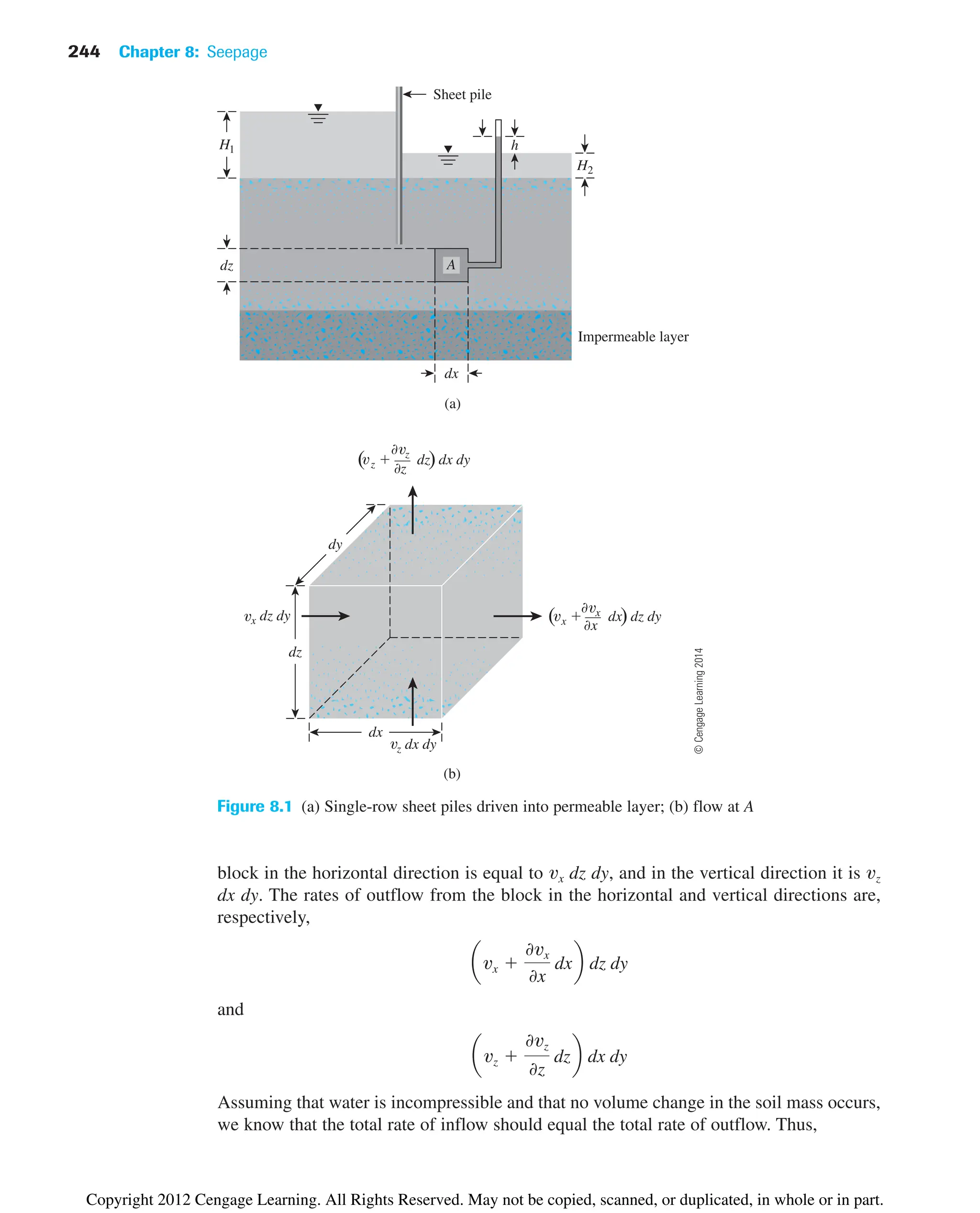
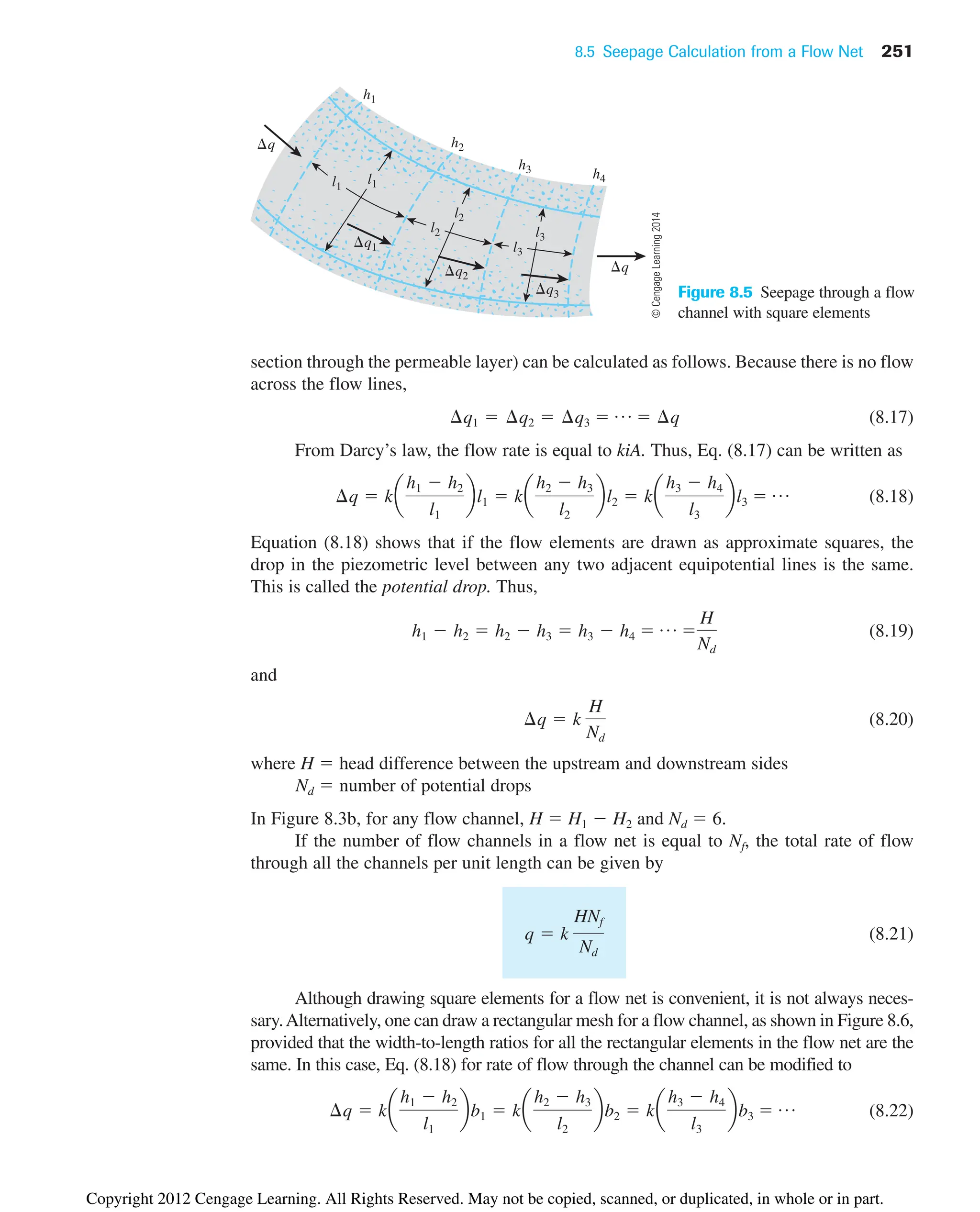
![8.3 Continuity Equation for Solution of Simple Flow Problems 245
or
(8.1)
With Darcy’s law, the discharge velocities can be expressed as
(8.2)
and
(8.3)
where kx and kz are the hydraulic conductivities in the horizontal and vertical directions,
respectively.
From Eqs. (8.1), (8.2), and (8.3), we can write
(8.4)
If the soil is isotropic with respect to the hydraulic conductivity—that is, kx kz—the
preceding continuity equation for two-dimensional flow simplifies to
(8.5)
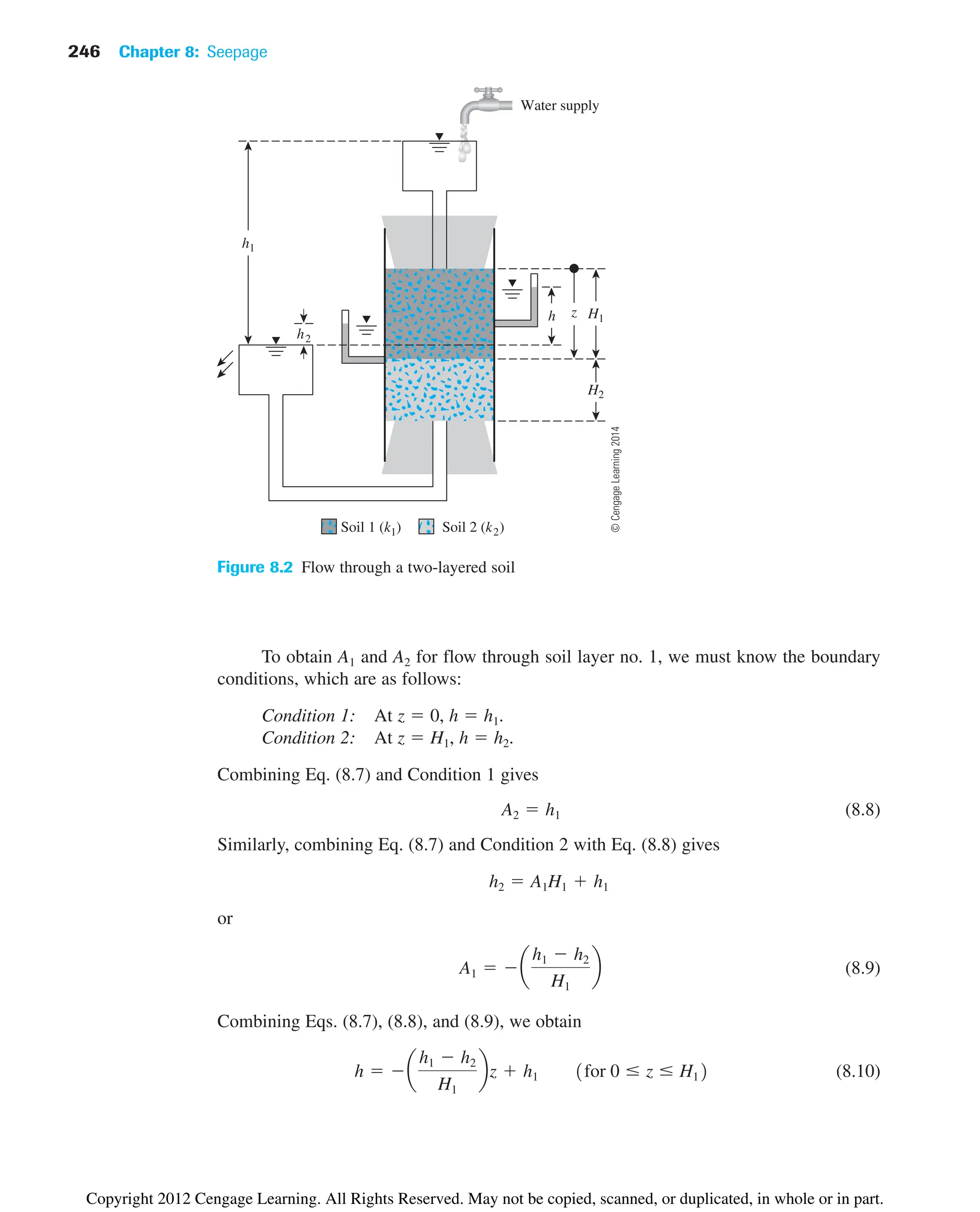
8.3 Continuity Equation for Solution
of Simple Flow Problems
The continuity equation given in Eq. (8.5) can be used in solving some simple flow problems.
To illustrate this, let us consider a one-dimensional flow problem, as shown in Figure 8.2, in
which a constant head is maintained across a two-layered soil for the flow of water. The head
difference between the top of soil layer no. 1 and the bottom of soil layer no. 2 is h1. Because
the flow is in only the z direction, the continuity equation [Eq. (8.5)] is simplified to the form
(8.6)
or
(8.7)
where A1 and A2 are constants.
h A1z A2
02
h
0z2
0
02
h
0x2
02
h
0z2
0
kx
02
h
0x2
kz
02
h
0z2
0
vz kziz kz
0h
0z
vx kxix kx
0h
0x
0vx
0x
0vz
0z
0
c avx
0vx
0x
dxb dz dy avz
0vz
0z
dzb dx dyd 3vx dz dy vz dx dy4 0
Copyright 2012 Cengage Learning. All Rights Reserved. May not be copied, scanned, or duplicated, in whole or in part.](https://image.slidesharecdn.com/principlesofgeotechnicalengineering-8thedition-231222125509-7e44d9bf/75/Principles-of-Geotechnical-Engineering-8th-Edition-pdf-265-2048.jpg)
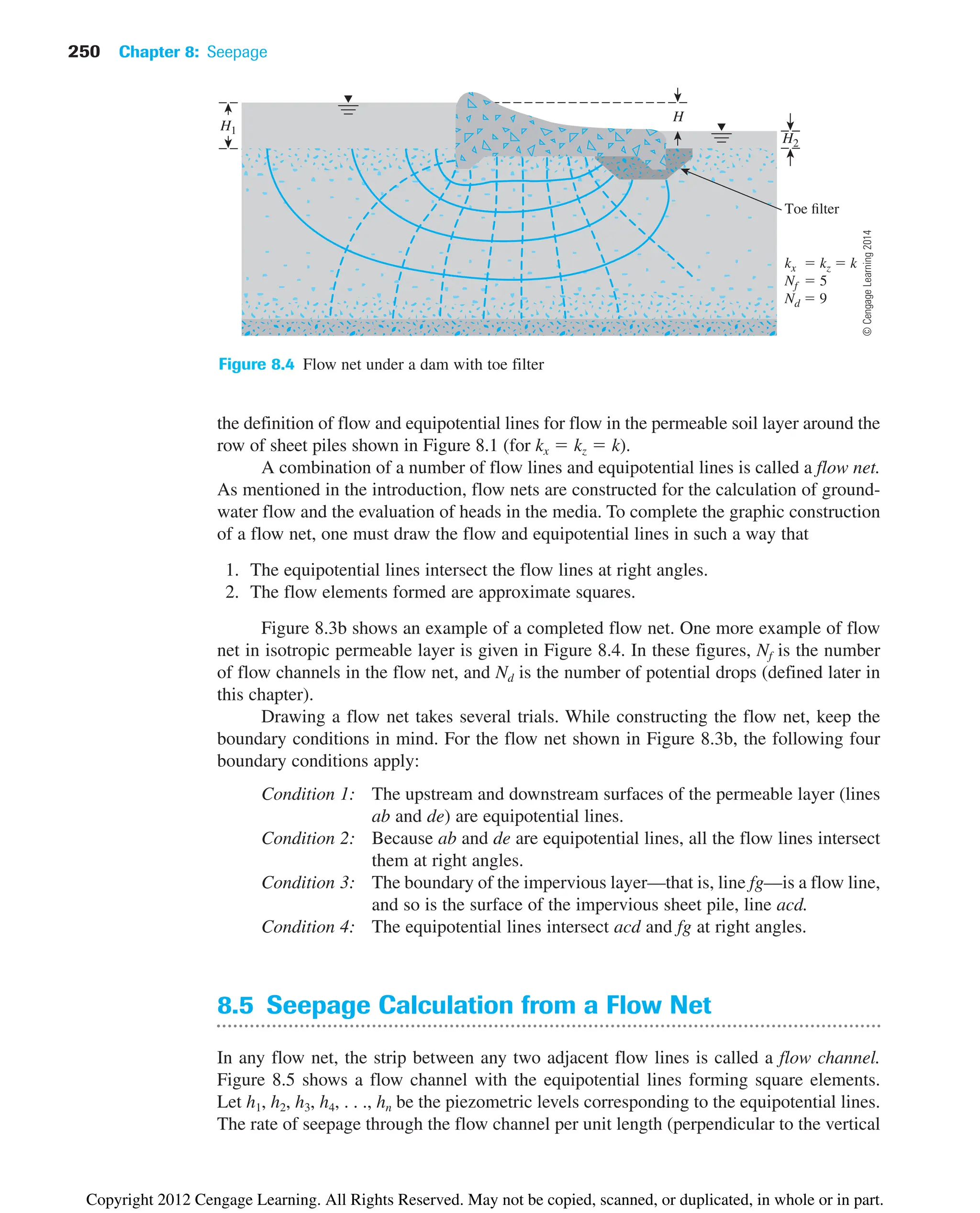
![8.4 Flow Nets 249
Impervious layer
Impervious layer
(a)
H1
H2
Equipotential line
Flow line
kx kz k
(b)
kx kz k
Nf 4
Nd 6
Water level
b a d e
Water level
c
f g
H1
H2
Sheet pile
Sheet pile
Figure 8.3 (a) Definition of flow lines and equipotential lines; (b) completed flow net
8.4 Flow Nets
The continuity equation [Eq. (8.5)] in an isotropic medium represents two orthogonal
families of curves—that is, the flow lines and the equipotential lines. A flow line is a line
along which a water particle will travel from upstream to the downstream side in the
permeable soil medium. An equipotential line is a line along which the potential head at all
points is equal. Thus, if piezometers are placed at different points along an equipotential
line, the water level will rise to the same elevation in all of them. Figure 8.3a demonstrates
©
Cengage
Learning
2014
Copyright 2012 Cengage Learning. All Rights Reserved. May not be copied, scanned, or duplicated, in whole or in part.](https://image.slidesharecdn.com/principlesofgeotechnicalengineering-8thedition-231222125509-7e44d9bf/75/Principles-of-Geotechnical-Engineering-8th-Edition-pdf-269-2048.jpg)
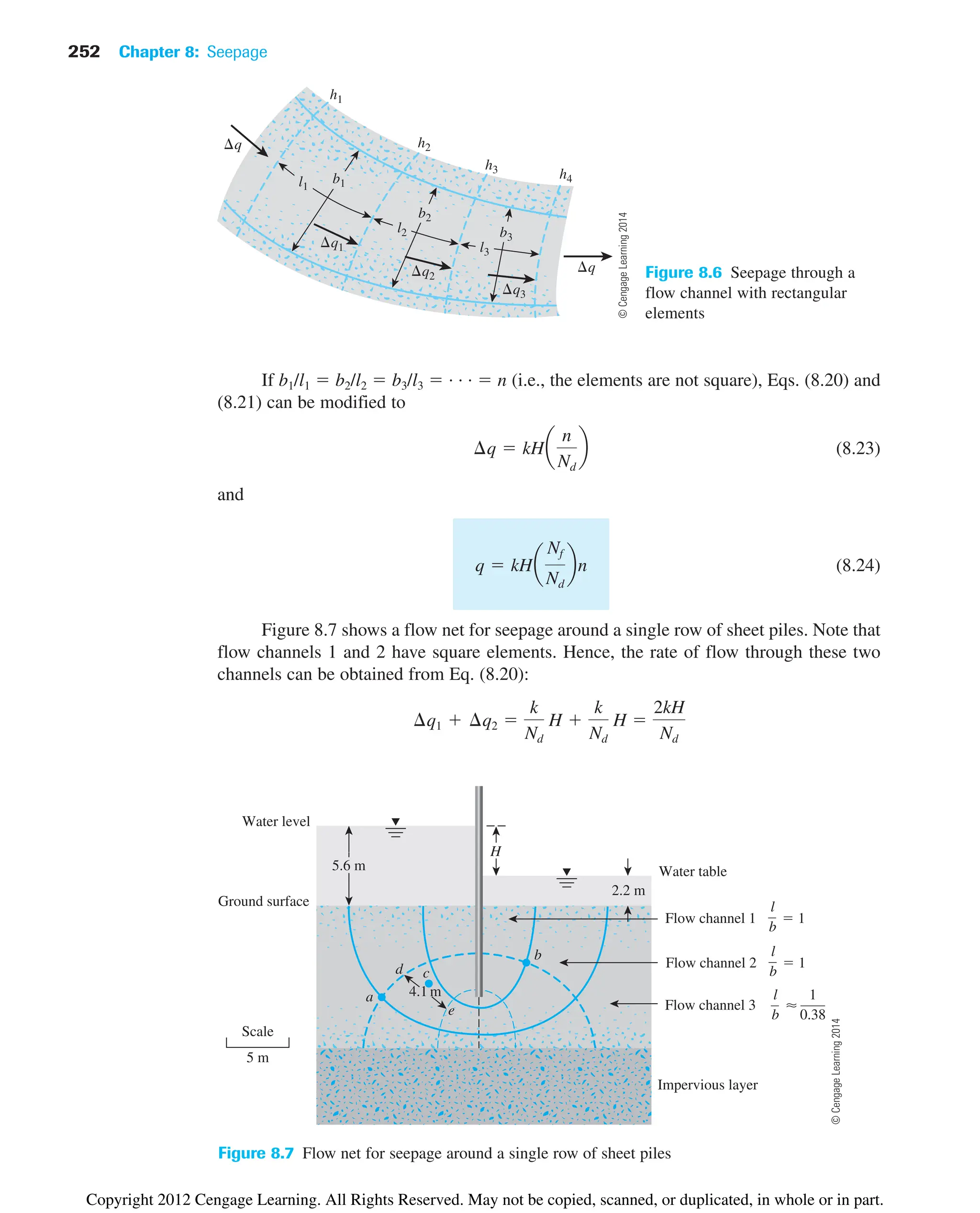
![254 Chapter 8: Seepage
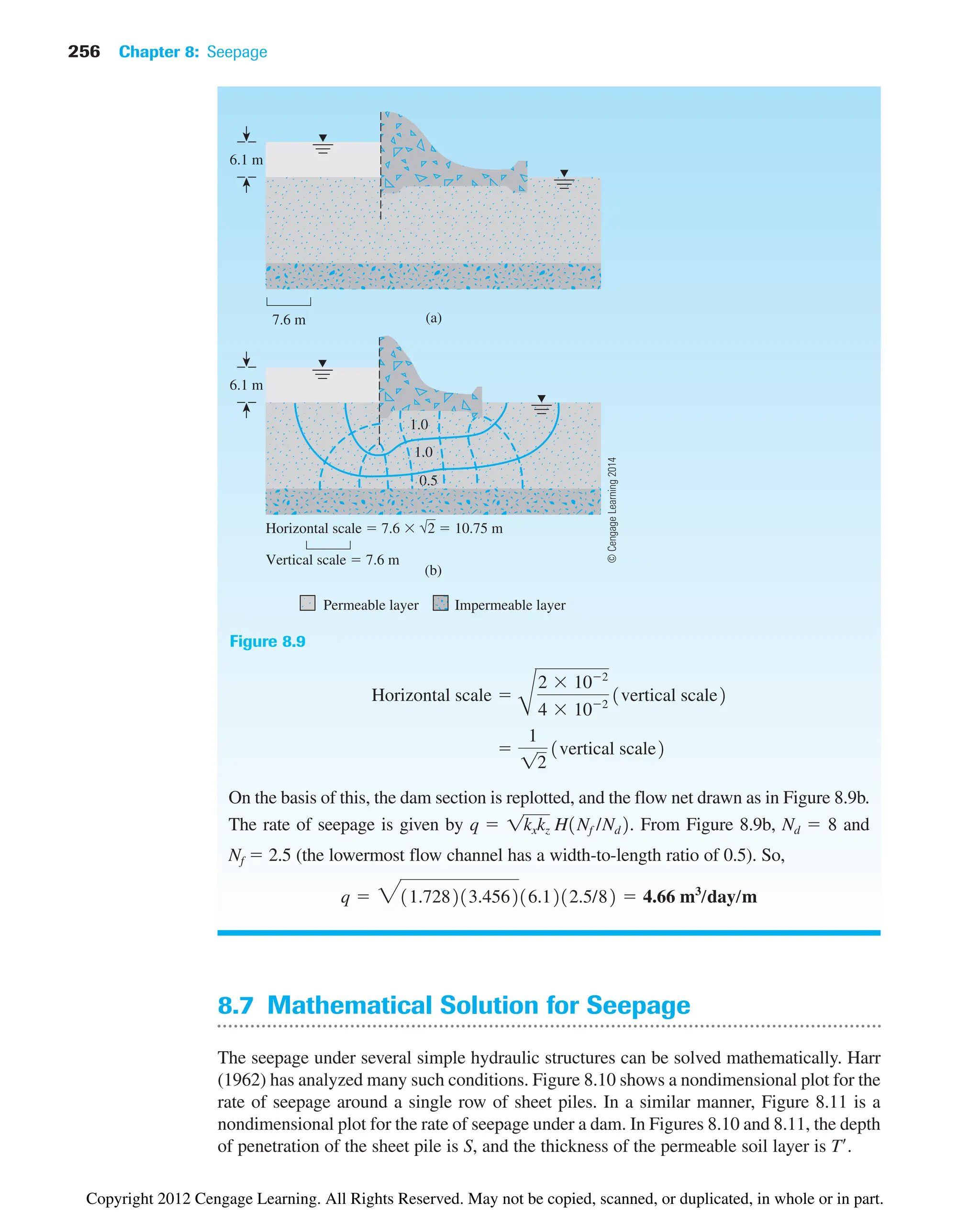
8.6 Flow Nets in Anisotropic Soil
The flow-net construction described thus far and the derived Eqs. (8.21) and (8.24) for
seepage calculation have been based on the assumption that the soil is isotropic. However,
in nature, most soils exhibit some degree of anisotropy. To account for soil anisotropy with
respect to hydraulic conductivity, we must modify the flow net construction.
The differential equation of continuity for a two-dimensional flow [Eq. (8.4)] is
For anisotropic soils, kx ⬆ kz. In this case, the equation represents two families of
curves that do not meet at 90°. However, we can rewrite the preceding equation as
(8.26)
Substituting we can express Eq. (8.26) as
(8.27)
Now Eq. (8.27) is in a form similar to that of Eq. (8.5), with x replaced by x, which is the
new transformed coordinate. To construct the flow net, use the following procedure:
Step 1: Adopt a vertical scale (that is, z axis) for drawing the cross section.
Step 2: Adopt a horizontal scale (that is, x axis) such that horizontal scale
vertical scale.
Step 3: With scales adopted as in steps 1 and 2, plot the vertical section through the
permeable layer parallel to the direction of flow.
Step 4: Draw the flow net for the permeable layer on the section obtained from
step 3, with flow lines intersecting equipotential lines at right angles and the
elements as approximate squares.
The rate of seepage per unit length can be calculated by modifying Eq. (8.21) to
(8.28)
where H total head loss
Nf and Nd number of flow channels and potential drops, respectively (from
flow net drawn in step 4)
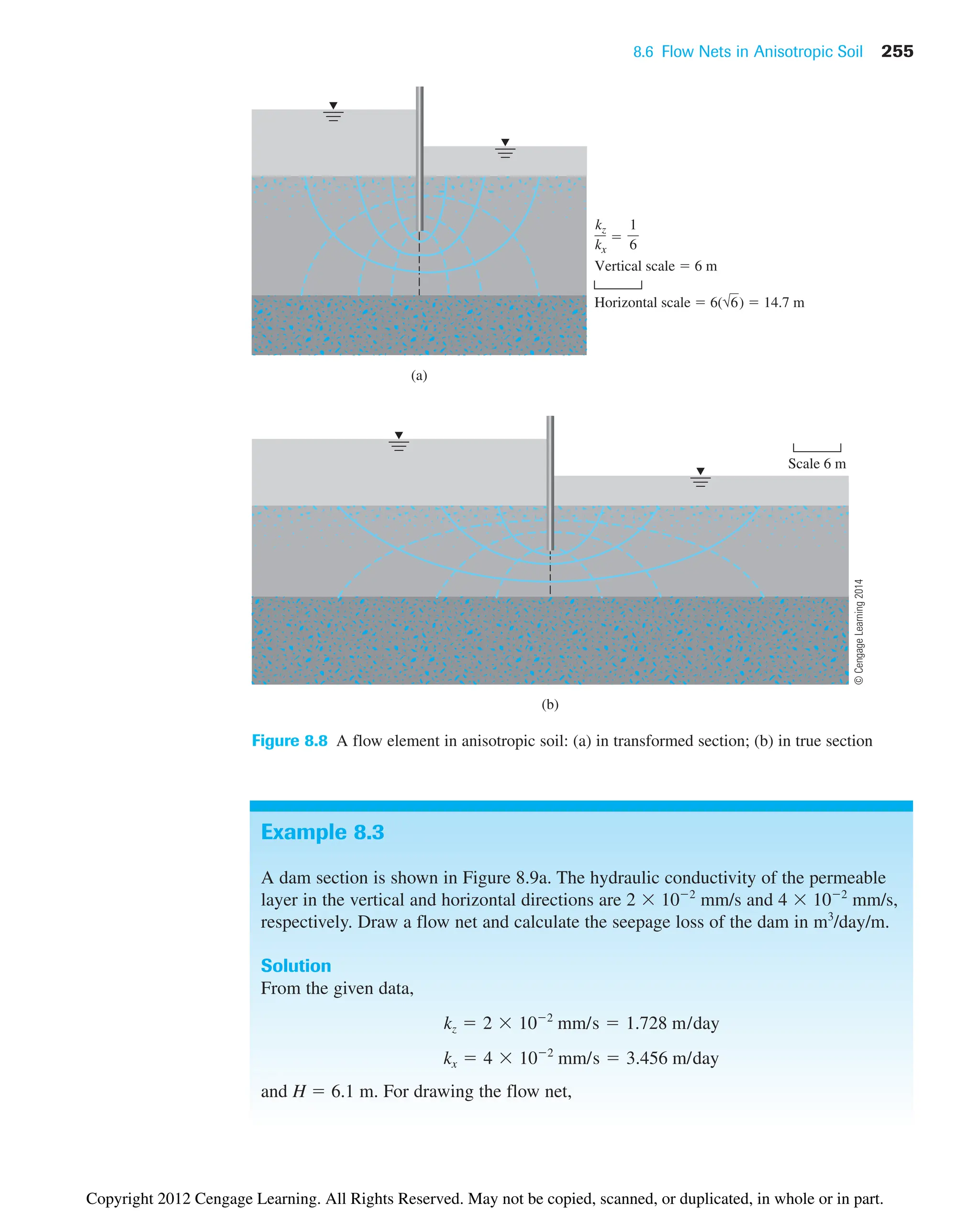
Note that when flow nets are drawn in transformed sections (in anisotropic soils),
the flow lines and the equipotential lines are orthogonal. However, when they are
redrawn in a true section, these lines are not at right angles to each other. This fact is
shown in Figure 8.8. In this figure, it is assumed that kx 6kz. Figure 8.8a shows a flow
element in a transformed section. The flow element has been redrawn in a true section
in Figure 8.8b.
q 2kx kz
HNf
Nd
3kz /kx
02
h
0x¿2
02
h
0z2
0
x¿ 1kz /kx x,
02
h
1kz /kx2 0x2
02
h
0z2
0
kx
02
h
0x2
kz
02
h
0z2
0
Copyright 2012 Cengage Learning. All Rights Reserved. May not be copied, scanned, or duplicated, in whole or in part.](https://image.slidesharecdn.com/principlesofgeotechnicalengineering-8thedition-231222125509-7e44d9bf/75/Principles-of-Geotechnical-Engineering-8th-Edition-pdf-274-2048.jpg)
![Problems 267
8.12 Summary
Following is a summary of the subjects covered in this chapter.
• In an isotropic soil, Laplace’s equation of continuity for two-dimensional flow is
given as [Eq. (8.5)]:
• A flow net is a combination of flow lines and equipotential lines that are two orthogonal
families of lines (Section 8.4).
• In an isotropic soil, seepage (q) for unit length of the structure in unit time can be
expressed as [Eq. (8.24)]
• The construction of flow nets in anisotropic soil was outlined in Section 8.6. For this
case, the seepage for unit length of the structure in unit time is [Eq. (8.28)]
• Seepage through an earth dam on an impervious base was discussed in Section 8.9
(Schaffernak’s solution with Casagrande’s correction) and Section 8.10 (L.
Casagrande solution).
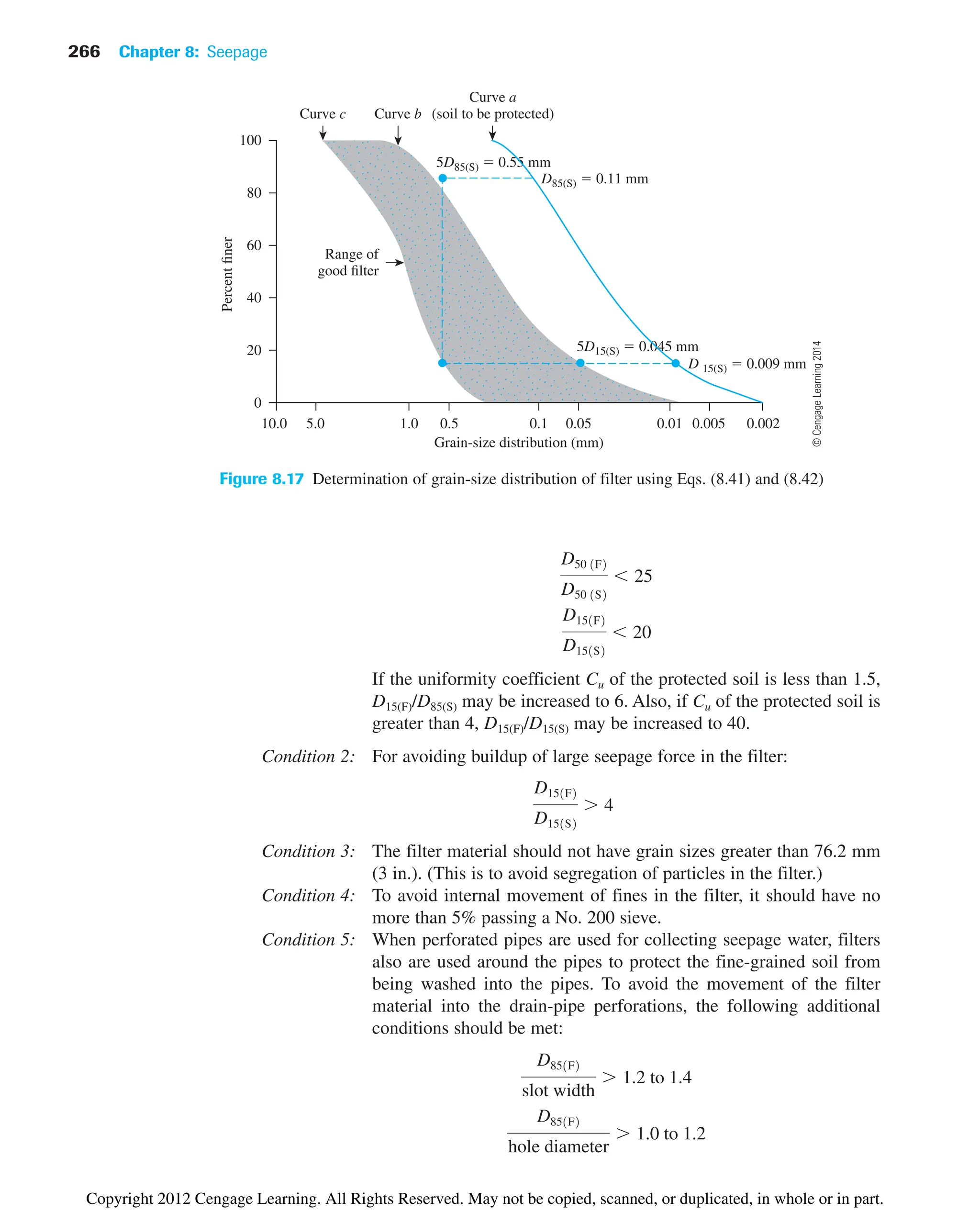
• The criteria for filter design are given in Section 8.11 [Eqs. (8.41) and (8.42)],
according to which
and
D151F2
D151S2
4 to 5
D151F2
D851S2
4 to 5
q 1kxkz
HNf
Nd
q kHa
Nf
Nd
bn
02
h
0x2
02
h
0z2
0
Problems
8.1 Refer to the constant-head permeability test arrangement in a two-layered soil as
shown in Figure 8.2. During the test, it was seen that when a constant head of
h1 200 mm was maintained, the magnitude of h2 was 80 mm. If k1 is 0.004 cm/sec,
determine the value of k2 given H1 100 mm and H2 150 mm.
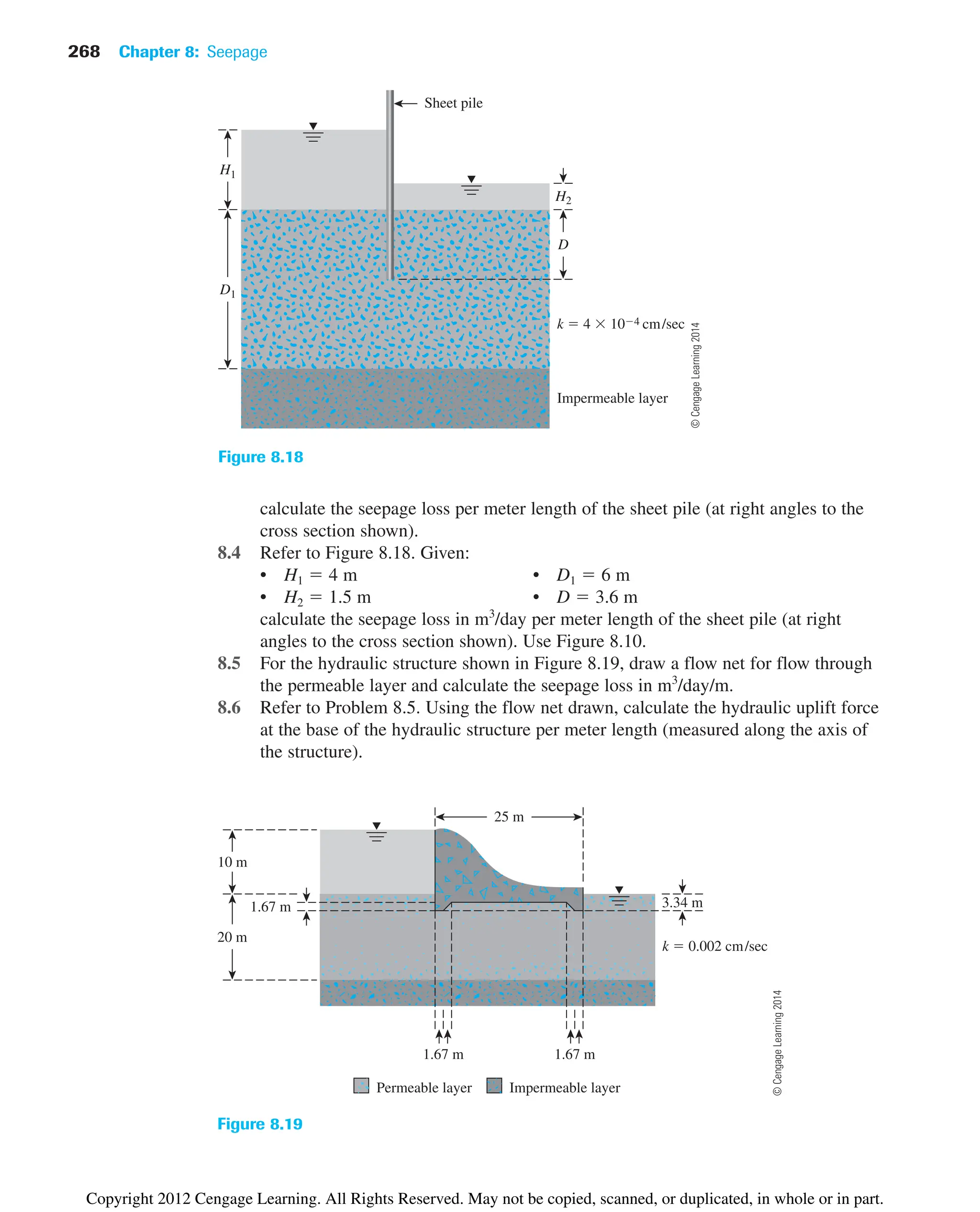
8.2 Refer to Figure 8.18. Given:
• H1 6 m • D 3 m
• H2 1.5 m • D1 6 m
draw a flow net. Calculate the seepage loss per meter length of the sheet pile (at a
right angle to the cross section shown).
8.3 Draw a flow net for the single row of sheet piles driven into a permeable layer as
shown in Figure 8.18. Given:
• H1 3 m • D 1.5 m
• H2 0.5 m • D1 3.75 m
Copyright 2012 Cengage Learning. All Rights Reserved. May not be copied, scanned, or duplicated, in whole or in part.](https://image.slidesharecdn.com/principlesofgeotechnicalengineering-8thedition-231222125509-7e44d9bf/75/Principles-of-Geotechnical-Engineering-8th-Edition-pdf-287-2048.jpg)
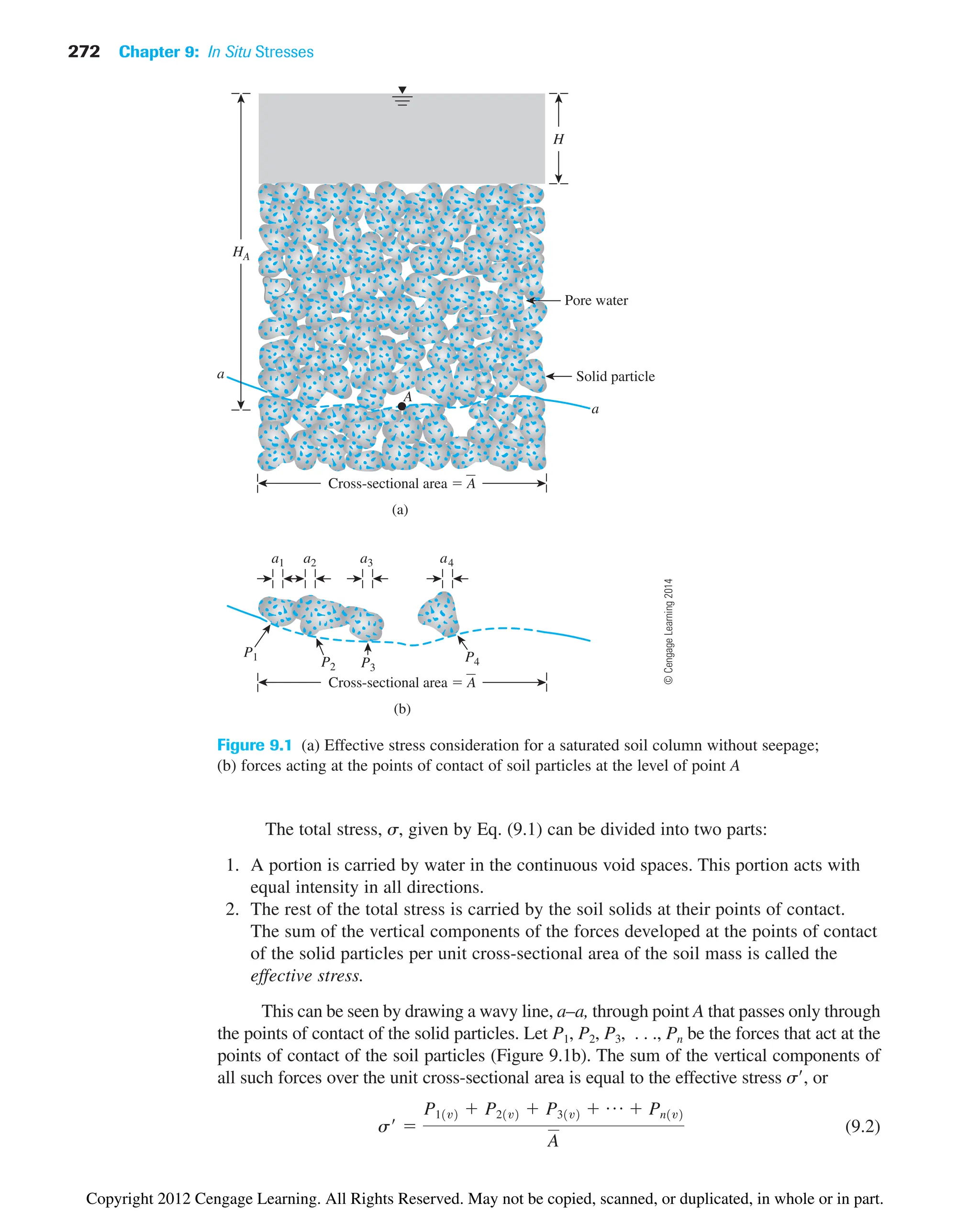
![9.2 Stresses in Saturated Soil without Seepage 273
where P1(v), P2(v), P3(v), . . ., Pn(v) are the vertical components of P1, P2, P3, . . ., Pn, respec-
tively, and is the cross-sectional area of the soil mass under consideration.
Again, if as is the cross-sectional area occupied by solid-to-solid contacts (that is,
as a1 a2 a3 . . . an), then the space occupied by water equals ( as). So we
can write
(9.3)
where u HA gw pore water pressure (that is, the hydrostatic pressure at A)
fraction of unit cross-sectional area of the soil mass occupied by
solid-to-solid contacts
The value of is extremely small and can be neglected for pressure ranges gener-
ally encountered in practical problems. Thus, Eq. (9.3) can be approximated by
(9.4)
where u is also referred to as neutral stress. Substitution of Eq. (9.1) for s in Eq. (9.4) gives
(9.5)
where g gsat gw equals the submerged unit weight of soil. Thus, we can see that the effec-
tive stress at any point A is independent of the depth of water, H, above the submerged soil.
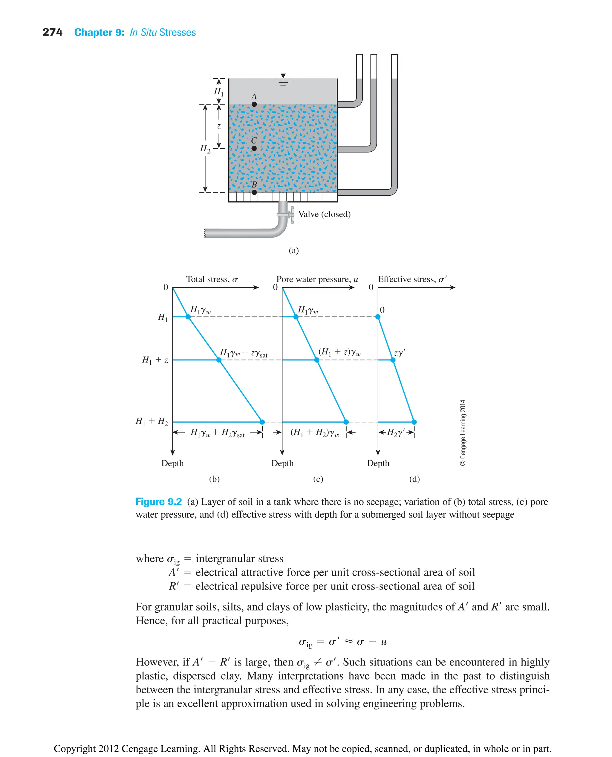
Figure 9.2a shows a layer of submerged soil in a tank where there is no seepage.
Figures 9.2b through 9.2d show plots of the variations of the total stress, pore water pres-
sure, and effective stress, respectively, with depth for a submerged layer of soil placed in
a tank with no seepage.
The principle of effective stress [Eq. (9.4)] was first developed by Terzaghi (1925,
1936). Skempton (1960) extended the work of Terzaghi and proposed the relationship
between total and effective stress in the form of Eq. (9.3).
In summary, effective stress is approximately the force per unit area carried by the
soil skeleton. The effective stress in a soil mass controls its volume change and strength.
Increasing the effective stress induces soil to move into a denser state of packing.
The effective stress principle is probably the most important concept in geotechnical
engineering. The compressibility and shearing resistance of a soil depend to a great extent on
the effective stress. Thus, the concept of effective stress is significant in solving geotechni-
cal engineering problems, such as the lateral earth pressure on retaining structures, the load-
bearing capacity and settlement of foundations, and the stability of earth slopes.
In Eq. (9.2), the effective stress, s, is defined as the sum of the vertical components
of all intergranular contact forces over a unit gross cross-sectional area. This definition is
mostly true for granular soils; however, for fine-grained soils, intergranular contact may
not physically be there, because the clay particles are surrounded by tightly held water
film. In a more general sense, Eq. (9.3) can be rewritten as
(9.6)
s sig u11 as
¿ 2 A¿ R¿
1Height of the soil column2 g¿
1HA H21gsat gw2
s¿ 3Hgw 1HA H2gsat4 HAgw
s s¿ u
as
¿
as
¿ as/A
s s¿
u1A as2
A
s¿ u11 aœ
s2
A
A
Copyright 2012 Cengage Learning. All Rights Reserved. May not be copied, scanned, or duplicated, in whole or in part.](https://image.slidesharecdn.com/principlesofgeotechnicalengineering-8thedition-231222125509-7e44d9bf/75/Principles-of-Geotechnical-Engineering-8th-Edition-pdf-293-2048.jpg)
![9.6 Heaving in Soil Due to Flow around Sheet Piles 287
H
D
B
Deep homogeneous soil
Figure 9.13 Hazra chart for iexit [see Eq. (9.25)] for dams constructed over deep homogeneous
deposits
H
iexit = —
Ndl
H Nd
= 8
l
Figure 9.12 Definition of iexit [Eq. (9.24a)]
C
B/D
Toe sheeting only
Heel and toe sheeting
1.5
1.0
0.5
0.0
iexit = C —
H
B
0 5 10 15
©
Cengage
Learning
2014
©
Cengage
Learning
2014
Copyright 2012 Cengage Learning. All Rights Reserved. May not be copied, scanned, or duplicated, in whole or in part.](https://image.slidesharecdn.com/principlesofgeotechnicalengineering-8thedition-231222125509-7e44d9bf/75/Principles-of-Geotechnical-Engineering-8th-Edition-pdf-307-2048.jpg)
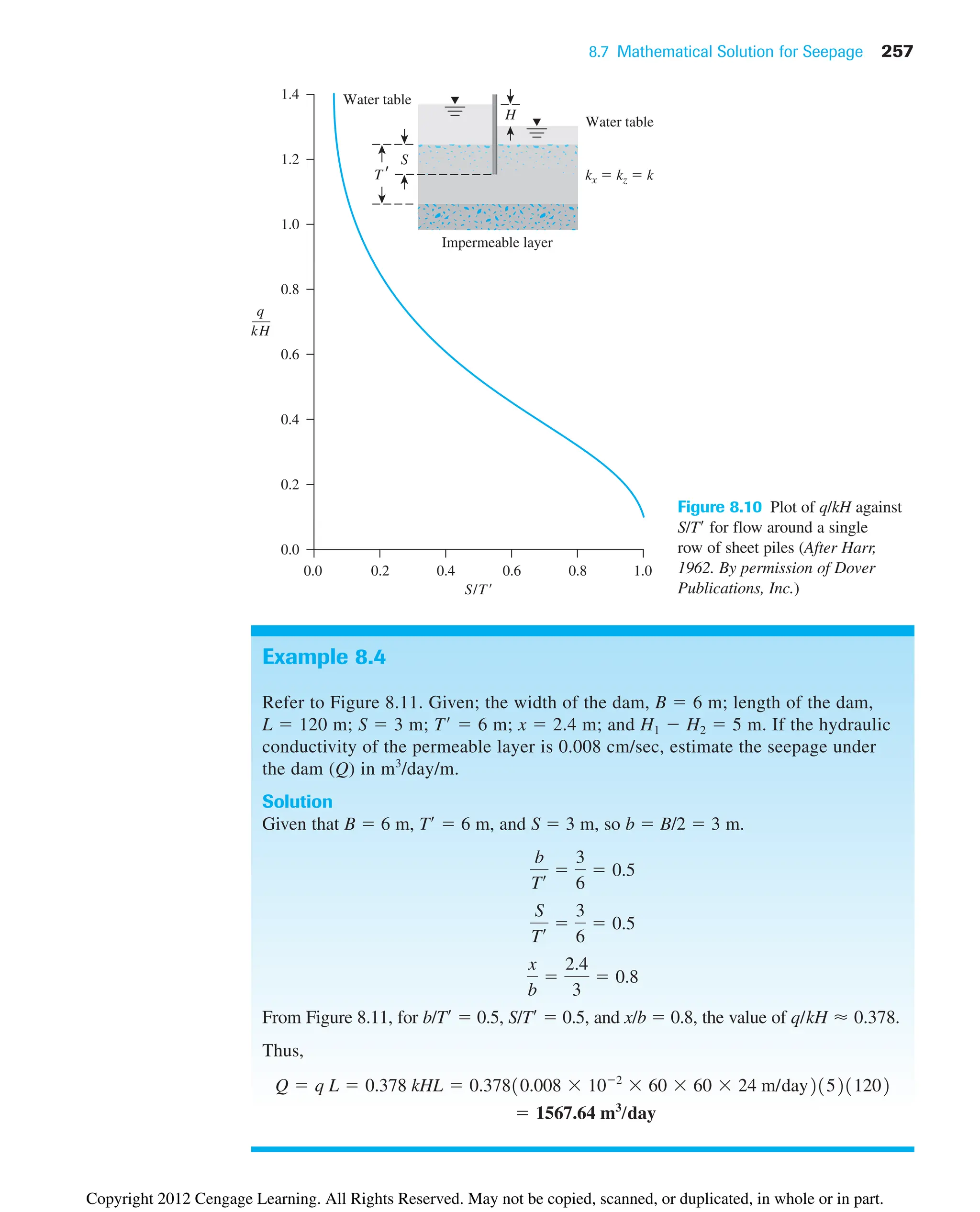
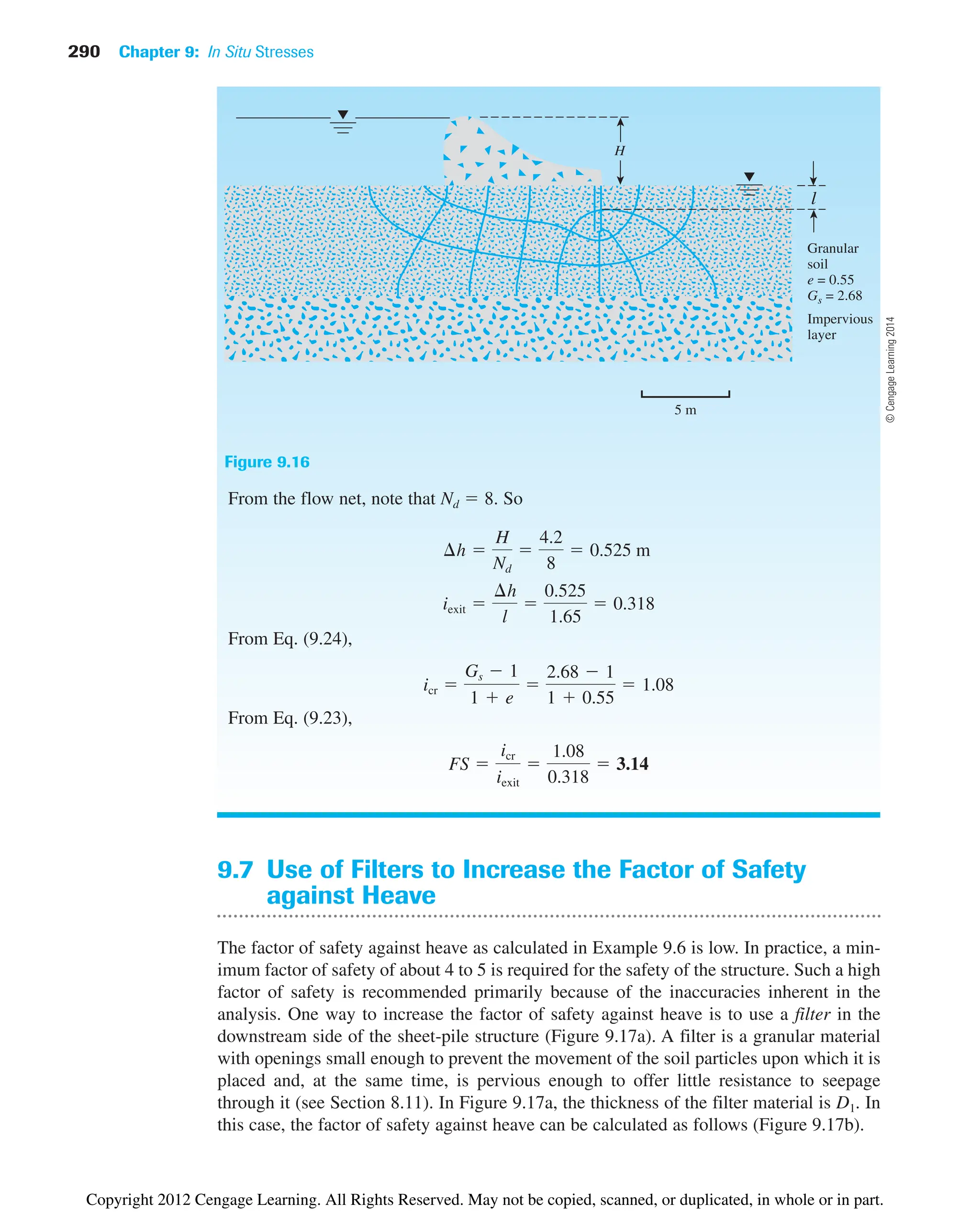
![9.6 Heaving in Soil Due to Flow around Sheet Piles 289
Example 9.7
Refer to Figure 9.16. For the flow under the weir, estimate the factor of safety against
piping.
Solution
We can scale the following:
l 1.65 m
H 4.2 m
Thus, the factor of safety [Eq. (9.20)] is
Alternate Solution
For this case, D/T 1/3. From Table 9.1, for D/T 1/3, the value of Co 0.357. Thus,
from Eq. (9.22),
FS
Dg¿
Cogw1H1 H22
162117.7 9.812
10.357219.812110 1.52
1.59
FS
g¿
iavgw
g¿D
0.361H1 H22gw
117.7 9.8126
0.36110 1.52 9.81
1.58
6 m
Driving
head
(H
1
H
2
)
Average 0.36
3 m
a d
b c
0
0.5
Soil prism
Figure 9.15 Soil prism—enlarged scale
©
Cengage
Learning
2014
Copyright 2012 Cengage Learning. All Rights Reserved. May not be copied, scanned, or duplicated, in whole or in part.](https://image.slidesharecdn.com/principlesofgeotechnicalengineering-8thedition-231222125509-7e44d9bf/75/Principles-of-Geotechnical-Engineering-8th-Edition-pdf-309-2048.jpg)
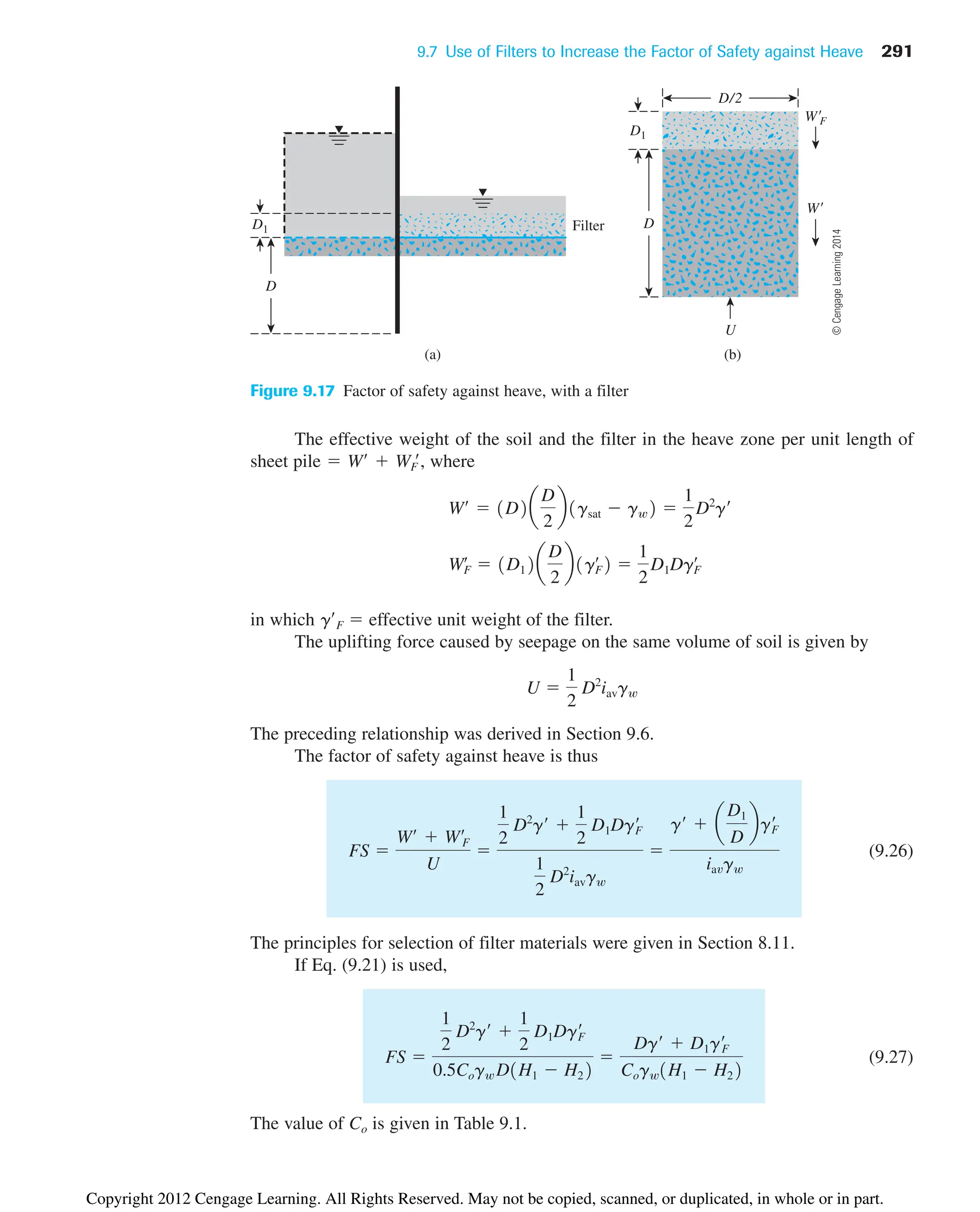
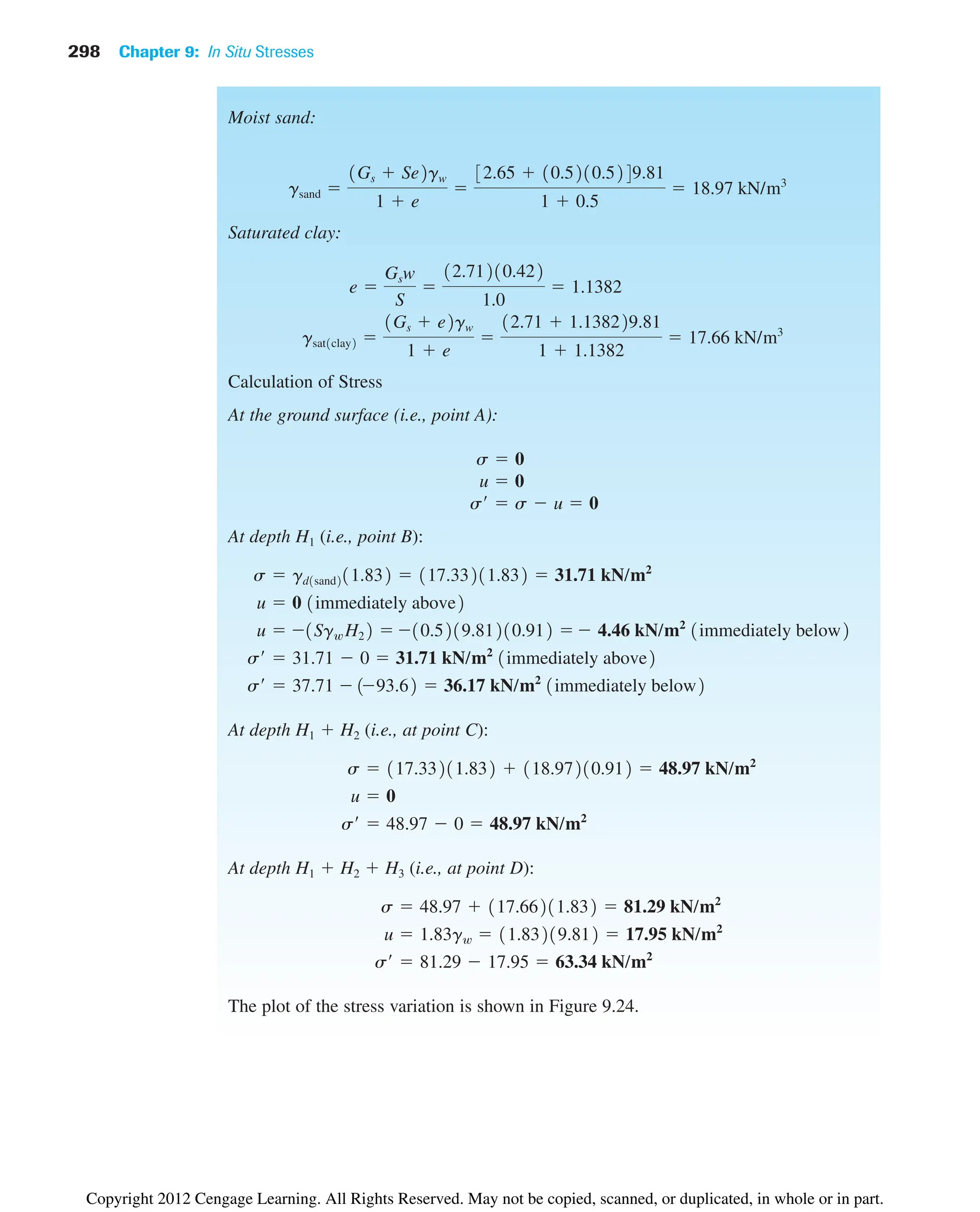
![9.11 Summary and General Comments 299
Figure 9.24
9.11 Summary and General Comments
The effective stress principle is probably the most important concept in geotechni-
cal engineering. The compressibility and shearing resistance of a soil depend to a
great extent on the effective stress. Thus, the concept of effective stress is signifi-
cant in solving geotechnical engineering problems, such as the lateral earth pressure
on retaining structures, the load-bearing capacity and settlement of foundations, and
the stability of earth slopes. Following is a summary of the topics discussed in this
chapter:
• The total stress (s) at a point in the soil mass is the sum of effective stress (s) and
pore water pressure (u), or [Eq. (9.4)]
• The critical hydraulic gradient (icr) for boiling or quick condition is given as
• Seepage force per unit volume in the direction of flow is equal to igw (i hydraulic
gradient in the direction of flow).
• The relationships to check for heaving for flow under a hydraulic structure are dis-
cussed in Section 9.6. Also, the possibility of using filters to increase the factor of
safety against heaving is discussed in Section 9.7.
icr
g¿
gw
effective unit weight of soil
unit weight of water
s s¿ u
©
Cengage
Learning
2014
0.0 0.0 0.0
0.0
1.83 36.17
48.97
63.34
31.71
1.83
2.74 2.74
4.57 4.57
17.95
−4.46
1.83
2.74
4.57
Depth (m) Depth (m) Depth (m)
81.29
48.97
31.71
σ (kN/m2) σ(kN/m2)
u (kN/m2)
Copyright 2012 Cengage Learning. All Rights Reserved. May not be copied, scanned, or duplicated, in whole or in part.](https://image.slidesharecdn.com/principlesofgeotechnicalengineering-8thedition-231222125509-7e44d9bf/75/Principles-of-Geotechnical-Engineering-8th-Edition-pdf-319-2048.jpg)
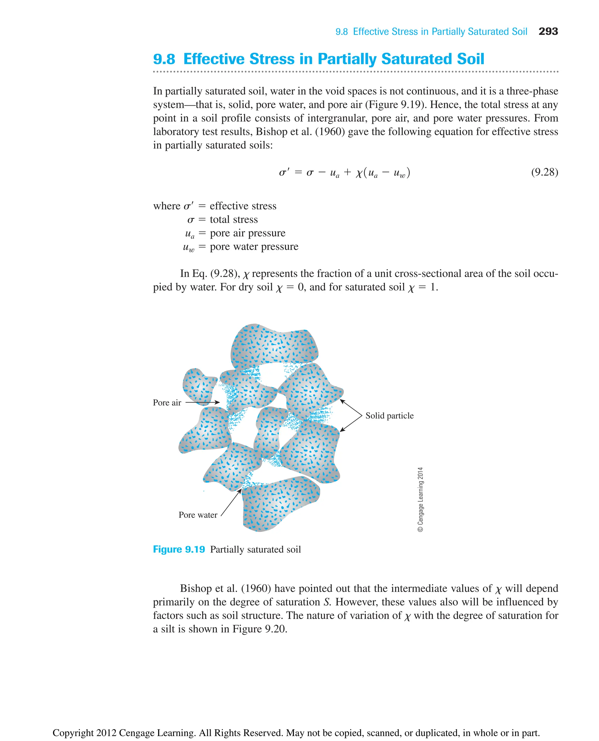
![• Effective stress at a point in a partially saturated soil can be expressed as [Eq. (9.28)]
where s total stress
ua, uw pore air and pore water pressure, respectively
x a factor which is zero for dry soil and 1 for saturated soil
• Capillary rise in soil has been discussed in Section 9.9. Capillary rise can range from
0.1 m to 0.2 m in coarse sand to 7.5 m to 23 m in clay.
s¿ s ua x1ua uw2
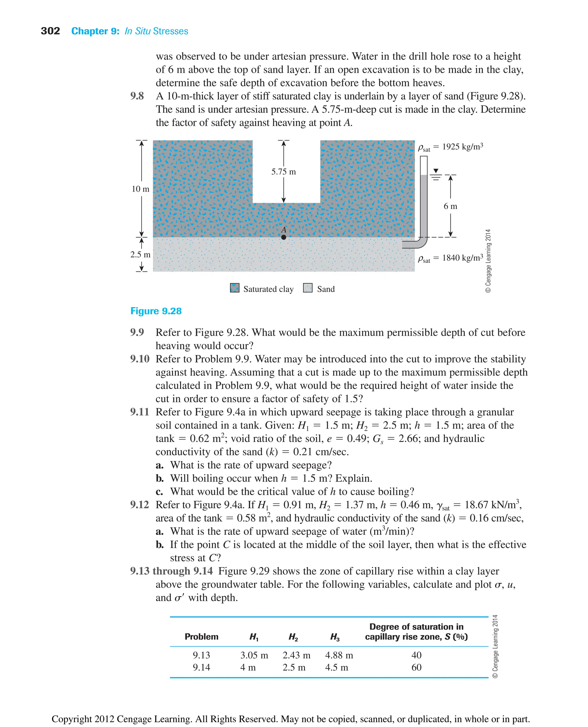
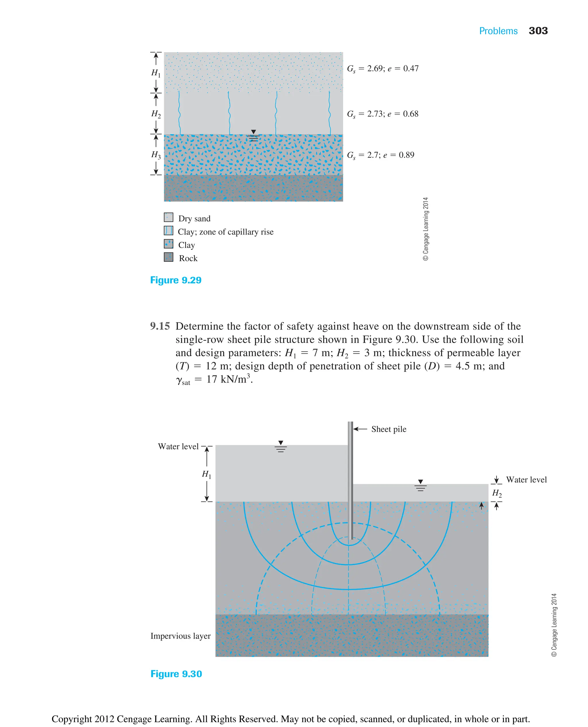
300 Chapter 9: In Situ Stresses
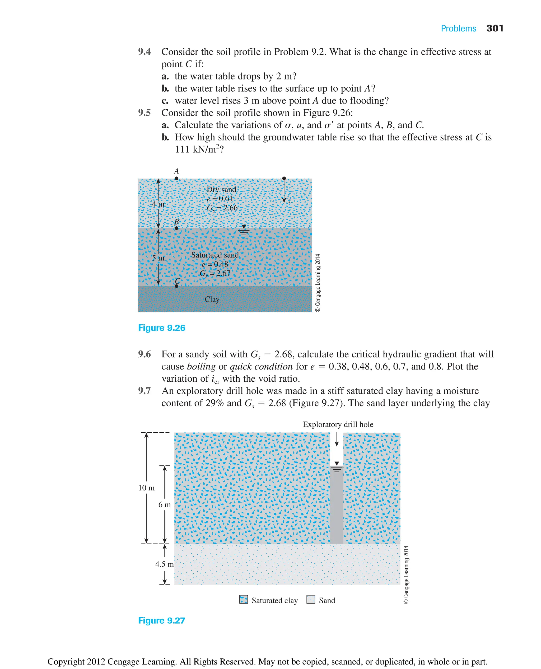
Problems
9.1 Through 9.3 A soil profile consisting of three layers is shown in Figure 9.25.
Calculate the values of s, u, and s at points A, B, C, and D for the following cases.
In each case, plot the variations of s, u, and s with depth. Characteristics
of layers 1, 2, and 3 for each case are given below:
B
H1
A
Groundwater table
Layer 1
Layer 2
Layer 3
H2
H3
Dry sand Clay Rock
Sand
C
D
Figure 9.25
Layer no. Thickness Soil parameters
9.1 1 H1 2.1 m gd 17.23 kN/m3
2 H2 3.66 m gsat 18.96 kN/m3
3 H3 1.83 m gsat 18.5 kN/m3
9.2 1 H1 5 m e 0.7; Gs 2.69
2 H2 8 m e 0.55; Gs 2.7
3 H3 3 m w 38%; e 1.2
9.3 1 H1 3 m gd 16 kN/m3
2 H2 6 m gsat 18 kN/m3
3 H3 2.5 m gsat 17 kN/m3
©
Cengage
Learning
2014
©
Cengage
Learning
2014
Copyright 2012 Cengage Learning. All Rights Reserved. May not be copied, scanned, or duplicated, in whole or in part.](https://image.slidesharecdn.com/principlesofgeotechnicalengineering-8thedition-231222125509-7e44d9bf/75/Principles-of-Geotechnical-Engineering-8th-Edition-pdf-320-2048.jpg)
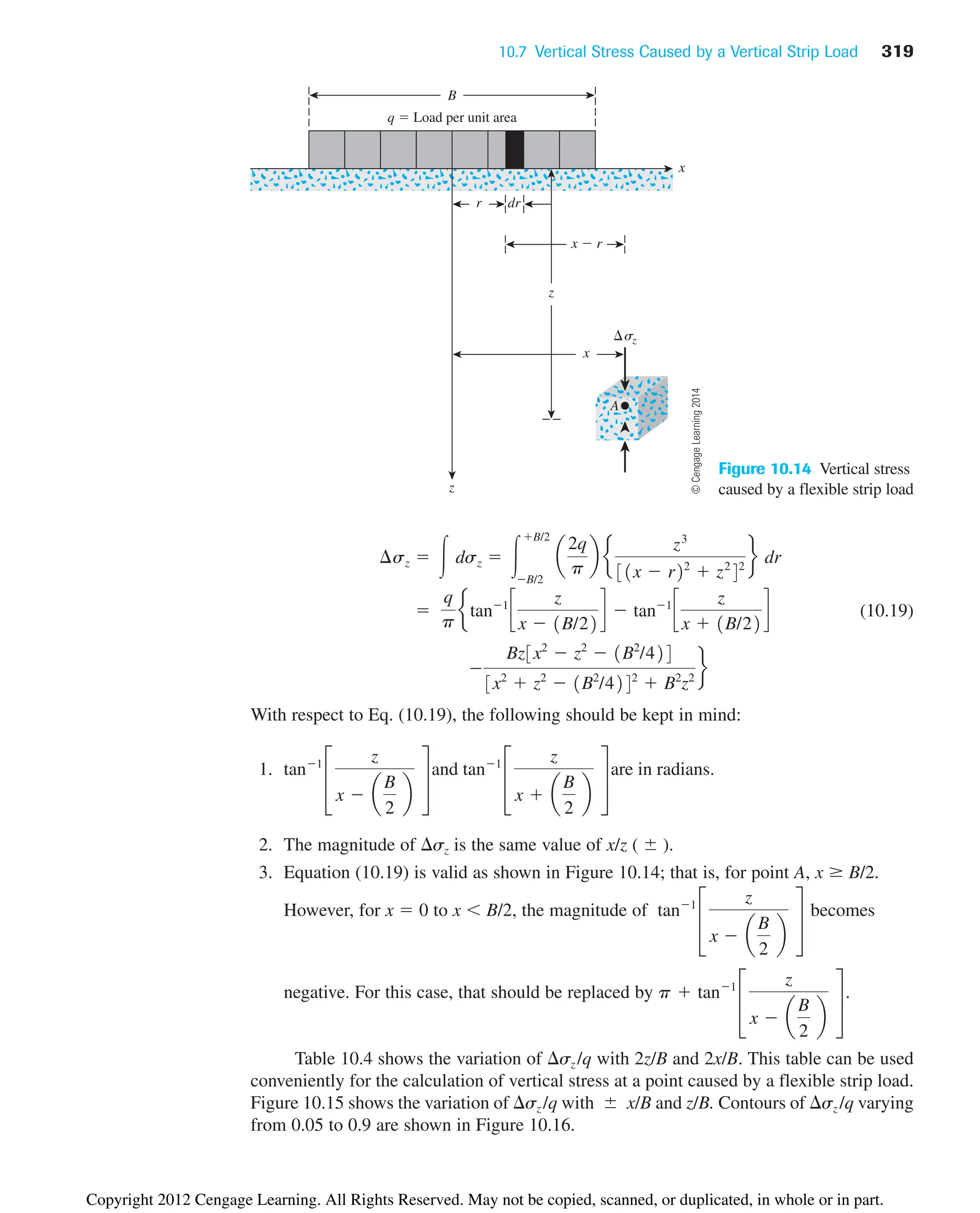
![308 Chapter 10: Stresses in a Soil Mass
Because the ordinates (that is, the shear stresses) of points N and S are zero, they rep-
resent the stresses on the principal planes. The abscissa of point N is equal to s1 [Eq.
(10.6)], and the abscissa for point S is s3 [Eq. (10.7)].
As a special case, if the planes AB and AD were major and minor principal planes,
the normal stress and the shear stress on plane EF could be found by substituting txy 0.
Equations (10.3) and (10.4) show that sy s1 and sx s3 (Figure 10.3a). Thus,
(10.8)
(10.9)
The Mohr’s circle for such stress conditions is shown in Figure 10.3b. The abscissa
and the ordinate of point Q give the normal stress and the shear stress, respectively, on the
plane EF.
tn
s1 s3
2
sin 2u
sn
s1 s3
2
s1 s3
2
cos 2u
Shear
stress,
t
Normal stress, s
S N
O
M
R (sx, txy)
s3
(sy,txy)
s1
Q
(sn, tn )
2u
√
s
x sy
2
2
txy
2
s
x sy
2 冢 冣
Figure 10.2
Principles of the Mohr’s circle
u
A B
C
D
E
F
(a)
s3
s3
s1
s1
(b)
Shear
stress
Normal stress
S N
s3
O
Q(sn, tn )
2u
s1
Figure 10.3 (a) Soil element with AB and AD as major and minor principal planes; (b) Mohr’s
circle for soil element shown in (a)
©
Cengage
Learning
2014
©
Cengage
Learning
2014
Copyright 2012 Cengage Learning. All Rights Reserved. May not be copied, scanned, or duplicated, in whole or in part.](https://image.slidesharecdn.com/principlesofgeotechnicalengineering-8thedition-231222125509-7e44d9bf/75/Principles-of-Geotechnical-Engineering-8th-Edition-pdf-328-2048.jpg)
![10.4 Stresses Caused by a Point Load 313
where
(10.14)
The variation of I1 for various values of r/z is given in Table 10.1. Figure 10.8 shows a plot
of I1 vs. r/z varying from zero to 1.5.
I1
3
2p
1
31r/z22
145/2
Table 10.1 Variation of I1 for Various Values of r/z [Eq. (10.14)]
r/z I1 r/z I1 r/z I1
0 0.4775 0.36 0.3521 1.80 0.0129
0.02 0.4770 0.38 0.3408 2.00 0.0085
0.04 0.4765 0.40 0.3294 2.20 0.0058
0.06 0.4723 0.45 0.3011 2.40 0.0040
0.08 0.4699 0.50 0.2733 2.60 0.0029
0.10 0.4657 0.55 0.2466 2.80 0.0021
0.12 0.4607 0.60 0.2214 3.00 0.0015
0.14 0.4548 0.65 0.1978 3.20 0.0011
0.16 0.4482 0.70 0.1762 3.40 0.00085
0.18 0.4409 0.75 0.1565 3.60 0.00066
0.20 0.4329 0.80 0.1386 3.80 0.00051
0.22 0.4242 0.85 0.1226 4.00 0.00040
0.24 0.4151 0.90 0.1083 4.20 0.00032
0.26 0.4050 0.95 0.0956 4.40 0.00026
0.28 0.3954 1.00 0.0844 4.60 0.00021
0.30 0.3849 1.20 0.0513 4.80 0.00017
0.32 0.3742 1.40 0.0317 5.00 0.00014
0.34 0.3632 1.60 0.0200
I1
r/z
0.2 0.4 0.6 0.8 1.0 1.2 1.4 1.5
0
0
0.1
0.2
0.3
0.4
0.5
Figure 10.8 Variation of I1 with r/z
©
Cengage
Learning
2014
©
Cengage
Learning
2014
Copyright 2012 Cengage Learning. All Rights Reserved. May not be copied, scanned, or duplicated, in whole or in part.](https://image.slidesharecdn.com/principlesofgeotechnicalengineering-8thedition-231222125509-7e44d9bf/75/Principles-of-Geotechnical-Engineering-8th-Edition-pdf-333-2048.jpg)
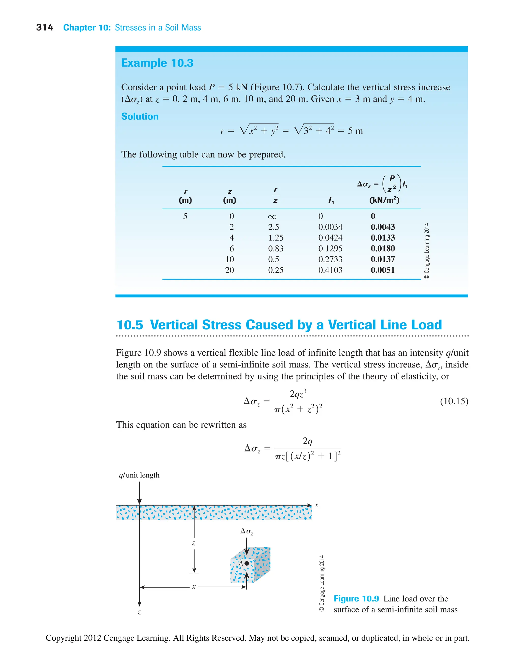
![10.5 Vertical Stress Caused by a Vertical Line Load 315
Table 10.2 Variation of sz/(q/z) with x/z [Eq. (10.16)]
x/z ⌬Sz /(q/z) x/z ⌬Sz /(q/z)
0 0.637
0.1 0.624
0.2 0.589
0.3 0.536
0.4 0.473
0.5 0.407
0.6 0.344
0.7 0.287
0.8 0.237
0.9 0.194
1.0 0.159
1.1 0.130
1.2 0.107
1.3 0.088
1.4 0.073
1.5 0.060
1.6 0.050
1.7 0.042
1.8 0.035
1.9 0.030
2.0 0.025
2.2 0.019
2.4 0.014
2.6 0.011
2.8 0.008
3.0 0.006
or
(10.16)
Note that Eq. (10.16) is in a nondimensional form. Using this equation, we can calculate
the variation of sz /(q/z) with x/z. This is given in Table 10.2. The value of sz calculated
by using Eq. (10.16) is the additional stress on soil caused by the line load. The value of
sz does not include the overburden pressure of the soil above point A. Figure 10.10 shows
a plot of sz/(q/z) vs. x/z.
¢sz
1q/z2
2
p31x/z22
142
Figure 10.10
Plot of this variation of
sz /(q/z) with (x/z)
≤ (x/z)
0.4 0.8 1.2 1.6 2.0 2.4 2.8 3.0
0
0
0.1
0.2
0.3
0.4
0.7
0.5
0.6
z
/(q/z)
©
Cengage
Learning
2014
©
Cengage
Learning
2014
Copyright 2012 Cengage Learning. All Rights Reserved. May not be copied, scanned, or duplicated, in whole or in part.](https://image.slidesharecdn.com/principlesofgeotechnicalengineering-8thedition-231222125509-7e44d9bf/75/Principles-of-Geotechnical-Engineering-8th-Edition-pdf-335-2048.jpg)
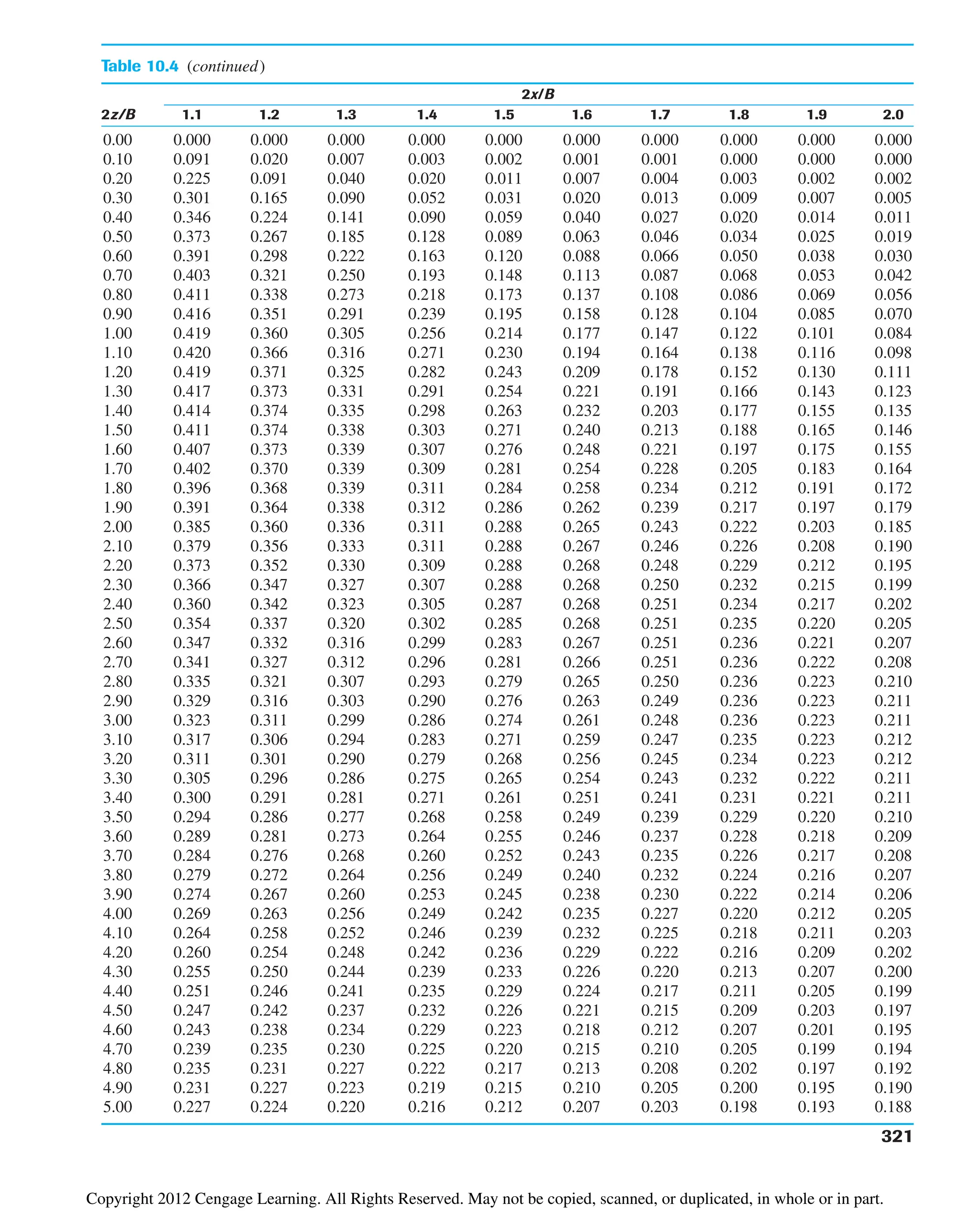
![Table 10.4 Variation of sz/q with 2z/B and 2x/B [Eq. (10.19)]
2x/B
2z/B 0.0 0.1 0.2 0.3 0.4 0.5 0.6 0.7 0.8 0.9 1.0
0.00 1.000 1.000 1.000 1.000 1.000 1.000 1.000 1.000 1.000 1.000 0.000
0.10 1.000 1.000 0.999 0.999 0.999 0.998 0.997 0.993 0.980 0.909 0.500
0.20 0.997 0.997 0.996 0.995 0.992 0.988 0.979 0.959 0.909 0.775 0.500
0.30 0.990 0.989 0.987 0.984 0.978 0.967 0.947 0.908 0.833 0.697 0.499
0.40 0.977 0.976 0.973 0.966 0.955 0.937 0.906 0.855 0.773 0.651 0.498
0.50 0.959 0.958 0.953 0.943 0.927 0.902 0.864 0.808 0.727 0.620 0.497
0.60 0.937 0.935 0.928 0.915 0.896 0.866 0.825 0.767 0.691 0.598 0.495
0.70 0.910 0.908 0.899 0.885 0.863 0.831 0.788 0.732 0.662 0.581 0.492
0.80 0.881 0.878 0.869 0.853 0.829 0.797 0.755 0.701 0.638 0.566 0.489
0.90 0.850 0.847 0.837 0.821 0.797 0.765 0.724 0.675 0.617 0.552 0.485
1.00 0.818 0.815 0.805 0.789 0.766 0.735 0.696 0.650 0.598 0.540 0.480
1.10 0.787 0.783 0.774 0.758 0.735 0.706 0.670 0.628 0.580 0.529 0.474
1.20 0.755 0.752 0.743 0.728 0.707 0.679 0.646 0.607 0.564 0.517 0.468
1.30 0.725 0.722 0.714 0.699 0.679 0.654 0.623 0.588 0.548 0.506 0.462
1.40 0.696 0.693 0.685 0.672 0.653 0.630 0.602 0.569 0.534 0.495 0.455
1.50 0.668 0.666 0.658 0.646 0.629 0.607 0.581 0.552 0.519 0.484 0.448
1.60 0.642 0.639 0.633 0.621 0.605 0.586 0.562 0.535 0.506 0.474 0.440
1.70 0.617 0.615 0.608 0.598 0.583 0.565 0.544 0.519 0.492 0.463 0.433
1.80 0.593 0.591 0.585 0.576 0.563 0.546 0.526 0.504 0.479 0.453 0.425
1.90 0.571 0.569 0.564 0.555 0.543 0.528 0.510 0.489 0.467 0.443 0.417
2.00 0.550 0.548 0.543 0.535 0.524 0.510 0.494 0.475 0.455 0.433 0.409
2.10 0.530 0.529 0.524 0.517 0.507 0.494 0.479 0.462 0.443 0.423 0.401
2.20 0.511 0.510 0.506 0.499 0.490 0.479 0.465 0.449 0.432 0.413 0.393
2.30 0.494 0.493 0.489 0.483 0.474 0.464 0.451 0.437 0.421 0.404 0.385
2.40 0.477 0.476 0.473 0.467 0.460 0.450 0.438 0.425 0.410 0.395 0.378
2.50 0.462 0.461 0.458 0.452 0.445 0.436 0.426 0.414 0.400 0.386 0.370
2.60 0.447 0.446 0.443 0.439 0.432 0.424 0.414 0.403 0.390 0.377 0.363
2.70 0.433 0.432 0.430 0.425 0.419 0.412 0.403 0.393 0.381 0.369 0.355
2.80 0.420 0.419 0.417 0.413 0.407 0.400 0.392 0.383 0.372 0.360 0.348
2.90 0.408 0.407 0.405 0.401 0.396 0.389 0.382 0.373 0.363 0.352 0.341
3.00 0.396 0.395 0.393 0.390 0.385 0.379 0.372 0.364 0.355 0.345 0.334
3.10 0.385 0.384 0.382 0.379 0.375 0.369 0.363 0.355 0.347 0.337 0.327
3.20 0.374 0.373 0.372 0.369 0.365 0.360 0.354 0.347 0.339 0.330 0.321
3.30 0.364 0.363 0.362 0.359 0.355 0.351 0.345 0.339 0.331 0.323 0.315
3.40 0.354 0.354 0.352 0.350 0.346 0.342 0.337 0.331 0.324 0.316 0.308
3.50 0.345 0.345 0.343 0.341 0.338 0.334 0.329 0.323 0.317 0.310 0.302
3.60 0.337 0.336 0.335 0.333 0.330 0.326 0.321 0.316 0.310 0.304 0.297
3.70 0.328 0.328 0.327 0.325 0.322 0.318 0.314 0.309 0.304 0.298 0.291
3.80 0.320 0.320 0.319 0.317 0.315 0.311 0.307 0.303 0.297 0.292 0.285
3.90 0.313 0.313 0.312 0.310 0.307 0.304 0.301 0.296 0.291 0.286 0.280
4.00 0.306 0.305 0.304 0.303 0.301 0.298 0.294 0.290 0.285 0.280 0.275
4.10 0.299 0.299 0.298 0.296 0.294 0.291 0.288 0.284 0.280 0.275 0.270
4.20 0.292 0.292 0.291 0.290 0.288 0.285 0.282 0.278 0.274 0.270 0.265
4.30 0.286 0.286 0.285 0.283 0.282 0.279 0.276 0.273 0.269 0.265 0.260
4.40 0.280 0.280 0.279 0.278 0.276 0.274 0.271 0.268 0.264 0.260 0.256
4.50 0.274 0.274 0.273 0.272 0.270 0.268 0.266 0.263 0.259 0.255 0.251
4.60 0.268 0.268 0.268 0.266 0.265 0.263 0.260 0.258 0.254 0.251 0.247
4.70 0.263 0.263 0.262 0.261 0.260 0.258 0.255 0.253 0.250 0.246 0.243
4.80 0.258 0.258 0.257 0.256 0.255 0.253 0.251 0.248 0.245 0.242 0.239
4.90 0.253 0.253 0.252 0.251 0.250 0.248 0.246 0.244 0.241 0.238 0.235
5.00 0.248 0.248 0.247 0.246 0.245 0.244 0.242 0.239 0.237 0.234 0.231
320
©
Cengage
Learning
2014
Copyright 2012 Cengage Learning. All Rights Reserved. May not be copied, scanned, or duplicated, in whole or in part.](https://image.slidesharecdn.com/principlesofgeotechnicalengineering-8thedition-231222125509-7e44d9bf/75/Principles-of-Geotechnical-Engineering-8th-Edition-pdf-340-2048.jpg)
![322 Chapter 10: Stresses in a Soil Mass
≤ x/B
z/B = 0.25
2.0
1.0
0.5
0
0.2
0.4
0.6
1.0
0.8
0.2 0.4 0.6 1.0
0 0.8
z
/q
Figure 10.15 Variation of sz /q with z/B and x/B
[Eq. (10.19)]
B
2B
B/2
2B
0
B 3B
3B
4B
5B
6B
0.2
0.5
0.3
0.4
0.5
0.6
0.7
0.8
0.9
= 0.1
z /q
Figure 10.16 Contours of sz/q below a strip load
Example 10.6
Refer to Figure 10.14. Given: B 4 m and q 100 kN/m2
. For point A, z 1 m and
x 1 m. Determine the vertical stress sz at A. Use Eq. (10.19).
Solution
Since x 1 m B/2 2 m,
Bzcx2
z2
a
B2
4
b d
cx2
z2
a
B2
4
b d
2
B2
z2
∂
¢sz
q
p •
tan1
£
z
x a
B
2
b
§
p tan1
£
z
x a
B
2
b
§
©
Cengage
Learning
2014
©
Cengage
Learning
2014
Copyright 2012 Cengage Learning. All Rights Reserved. May not be copied, scanned, or duplicated, in whole or in part.](https://image.slidesharecdn.com/principlesofgeotechnicalengineering-8thedition-231222125509-7e44d9bf/75/Principles-of-Geotechnical-Engineering-8th-Edition-pdf-342-2048.jpg)
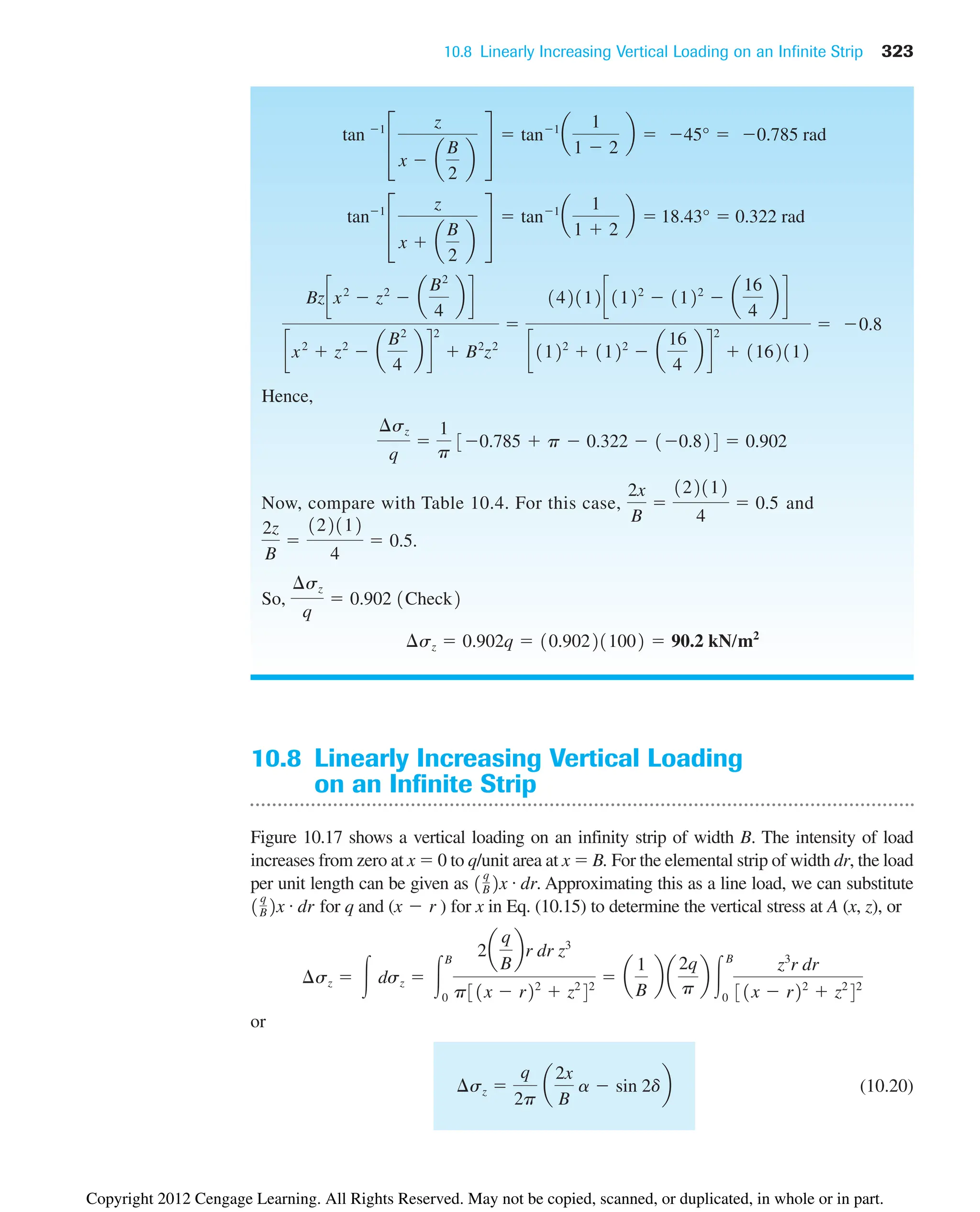
![324 Chapter 10: Stresses in a Soil Mass
Figure 10.17 Linearly increasing vertical loading on an infinite strip
Table 10.5 Variation of sz/q with 2x/B and 2 z/B [Eq. (10.20)]
2z/B
0 0.5 1.0 1.5 2.0 2.5 3.0 4.0 5.0
3 0 0.0003 0.0018 0.00054 0.0107 0.0170 0.0235 0.0347 0.0422
2 0 0.0008 0.0053 0.0140 0.0249 0.0356 0.0448 0.0567 0.0616
1 0 0.0041 0.0217 0.0447 0.0643 0.0777 0.0854 0.0894 0.0858
0 0 0.0748 0.1273 0.1528 0.1592 0.1553 0.1469 0.1273 0.1098
1 0.5 0.4797 0.4092 0.3341 0.2749 0.2309 0.1979 0.1735 0.1241
2 0.5 0.4220 0.3524 0.2952 0.2500 0.2148 0.1872 0.1476 0.1211
3 0 0.0152 0.0622 0.1010 0.1206 0.1268 0.1258 0.1154 0.1026
4 0 0.0019 0.0119 0.0285 0.0457 0.0596 0.0691 0.0775 0.0776
5 0 0.0005 0.0035 0.0097 0.0182 0.0274 0.0358 0.0482 0.0546
2x
B
In Eq. (10.20), a is in radians. Also. note the sign for the angle d. Table 10.5 shows
the variation of sz with 2x/B and 2z/B.
(x,z)
dr
x
z
q/unit area
r
α
+δ
Δσz
A
B
©
Cengage
Learning
2014
©
Cengage
Learning
2014
Copyright 2012 Cengage Learning. All Rights Reserved. May not be copied, scanned, or duplicated, in whole or in part.](https://image.slidesharecdn.com/principlesofgeotechnicalengineering-8thedition-231222125509-7e44d9bf/75/Principles-of-Geotechnical-Engineering-8th-Edition-pdf-344-2048.jpg)
![330 Chapter 10: Stresses in a Soil Mass
z
A
sz
Load per unit area q
r
dr
R
da
Figure 10.22 Vertical stress below the center of a
uniformly loaded flexible circular area
10.10 Vertical Stress below the Center of a Uniformly
Loaded Circular Area
Using Boussinesq’s solution for vertical stress sz caused by a point load [Eq. (10.12)],
one also can develop an expression for the vertical stress below the center of a uniformly
loaded flexible circular area.
From Figure 10.22, let the intensity of pressure on the circular area of radius R be
equal to q. The total load on the elemental area (shaded in the figure) is equal to qr dr da.
The vertical stress, dsz, at point A caused by the load on the elemental area (which may be
assumed to be a concentrated load) can be obtained from Eq. (10.12):
(10.25)
The increase in the stress at point A caused by the entire loaded area can be found
by integrating Eq. (10.25):
So,
(10.26)
¢sz qe1
1
31R/z22
143/2
f
¢sz 冮 dsz 冮
a2p
a0
冮
rR
r0
3q
2p
z3
r
1r2
z2
25/2
dr da
dsz
31qr dr da2
2p
z3
1r2
z2
25/2
©
Cengage
Learning
2014
Copyright 2012 Cengage Learning. All Rights Reserved. May not be copied, scanned, or duplicated, in whole or in part.](https://image.slidesharecdn.com/principlesofgeotechnicalengineering-8thedition-231222125509-7e44d9bf/75/Principles-of-Geotechnical-Engineering-8th-Edition-pdf-350-2048.jpg)
![10.11 Vertical Stress at Any Point below a Uniformly Loaded Circular Area 331
Table 10.6 Variation of sz/q with z/R [Eq. (10.26)]
z/R sz /q z/R sz /q
0 1 1.0 0.6465
0.02 0.9999 1.5 0.4240
0.05 0.9998 2.0 0.2845
0.10 0.9990 2.5 0.1996
0.2 0.9925 3.0 0.1436
0.4 0.9488 4.0 0.0869
0.5 0.9106 5.0 0.0571
0.8 0.7562
z
z
r
r sz
sz
A
q
R
Figure 10.23 Vertical stress at any point below
a uniformly loaded circular area
The variation of sz/q with z/R as obtained from Eq. (10.26) is given in Table 10.6.
The value of sz decreases rapidly with depth, and at z 5R, it is about 6% of q, which
is the intensity of pressure at the ground surface.
10.11 Vertical Stress at Any Point below a Uniformly
Loaded Circular Area
A detailed tabulation for calculation of vertical stress below a uniformly loaded flexible
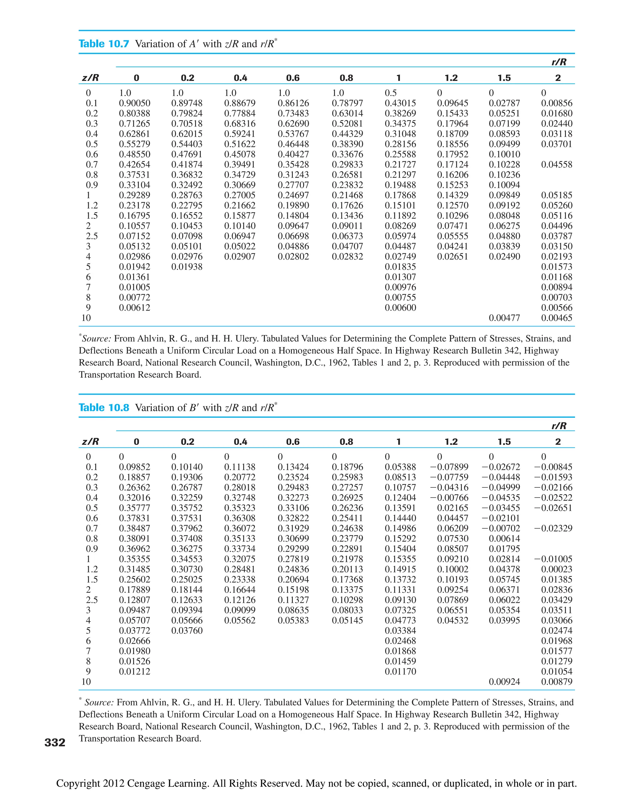
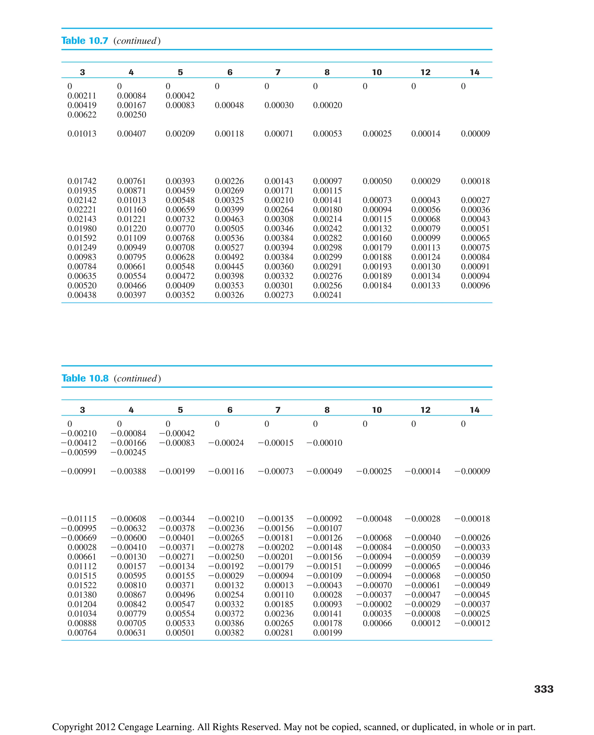
circular area was given by Ahlvin and Ulery (1962). Referring to Figure 10.23, we find that
sz at any point A located at a depth z at any distance r from the center of the loaded area
can be given as
(10.27)
where A and B are functions of z/R and r/R. (See Tables 10.7 and 10.8.) Figure 10.24
shows a plot of sz /q with r/R and z/R.
¢sz q1A¿ B¿2
©
Cengage
Learning
2014
©
Cengage
Learning
2014
Copyright 2012 Cengage Learning. All Rights Reserved. May not be copied, scanned, or duplicated, in whole or in part.](https://image.slidesharecdn.com/principlesofgeotechnicalengineering-8thedition-231222125509-7e44d9bf/75/Principles-of-Geotechnical-Engineering-8th-Edition-pdf-351-2048.jpg)
![334 Chapter 10: Stresses in a Soil Mass
1.0
0.8
0.6
0.8
0.6
r/R = 0
1.0
1.2
0.5
0.4
0.2
0
0 1 2
2.0
3
z/R
Δσ
z
/q
Figure 10.24
Plot of sz/q with
r/R and z/R
[Eq. (10.27)]
Example 10.9
Consider a uniformly loaded flexible circular area on the ground surface, as shown in
Fig. 10.23. Given: R 3 m and uniform load q 100 kN/m2
.
Calculate the increase in vertical stress at depths of 1.5 m, 3 m, 4.5 m, 6 m, and
12 m below the ground surface for points at (a) r 0 and (b) r 4.5 m.
©
Cengage
Learning
2014
Copyright 2012 Cengage Learning. All Rights Reserved. May not be copied, scanned, or duplicated, in whole or in part.](https://image.slidesharecdn.com/principlesofgeotechnicalengineering-8thedition-231222125509-7e44d9bf/75/Principles-of-Geotechnical-Engineering-8th-Edition-pdf-354-2048.jpg)
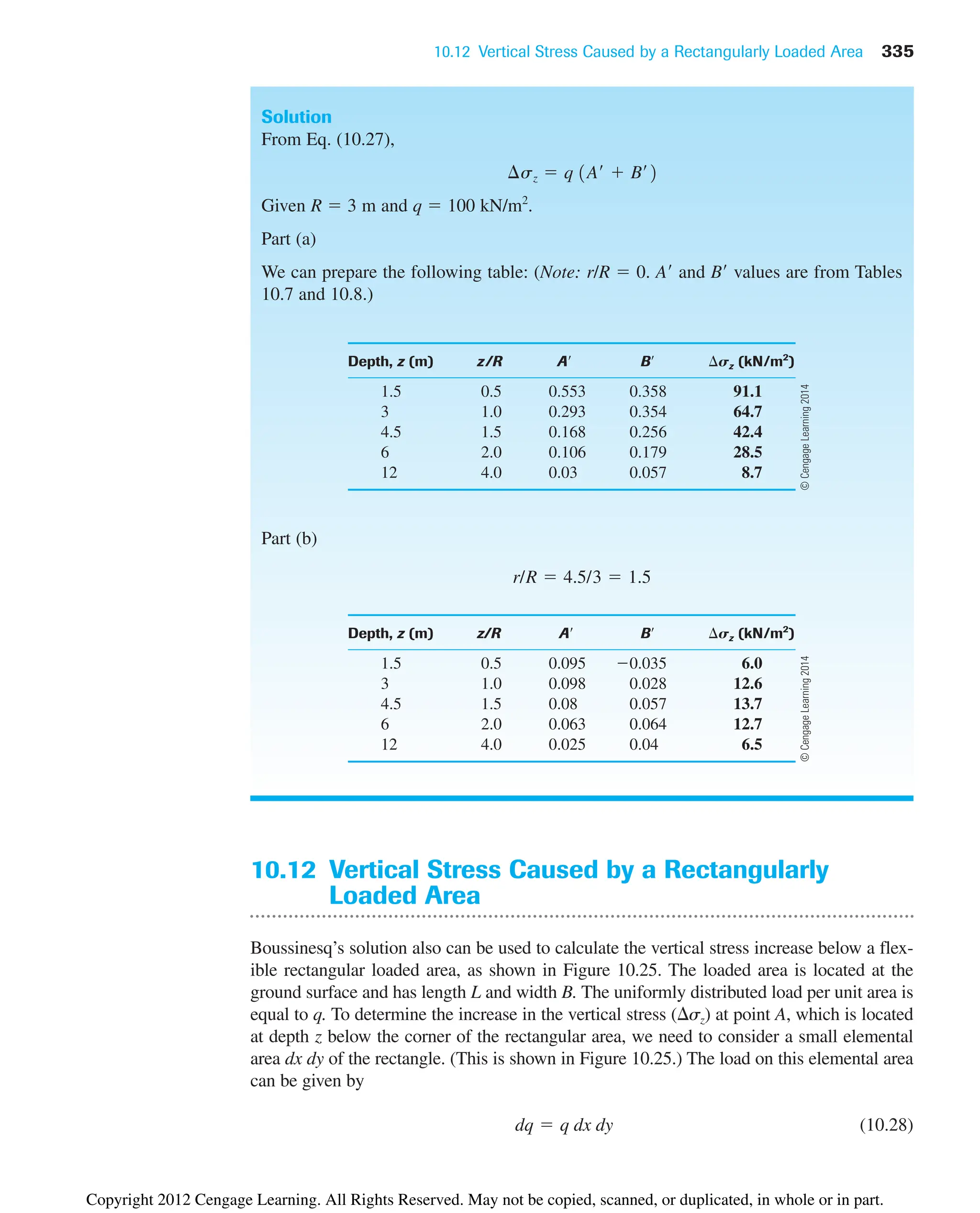
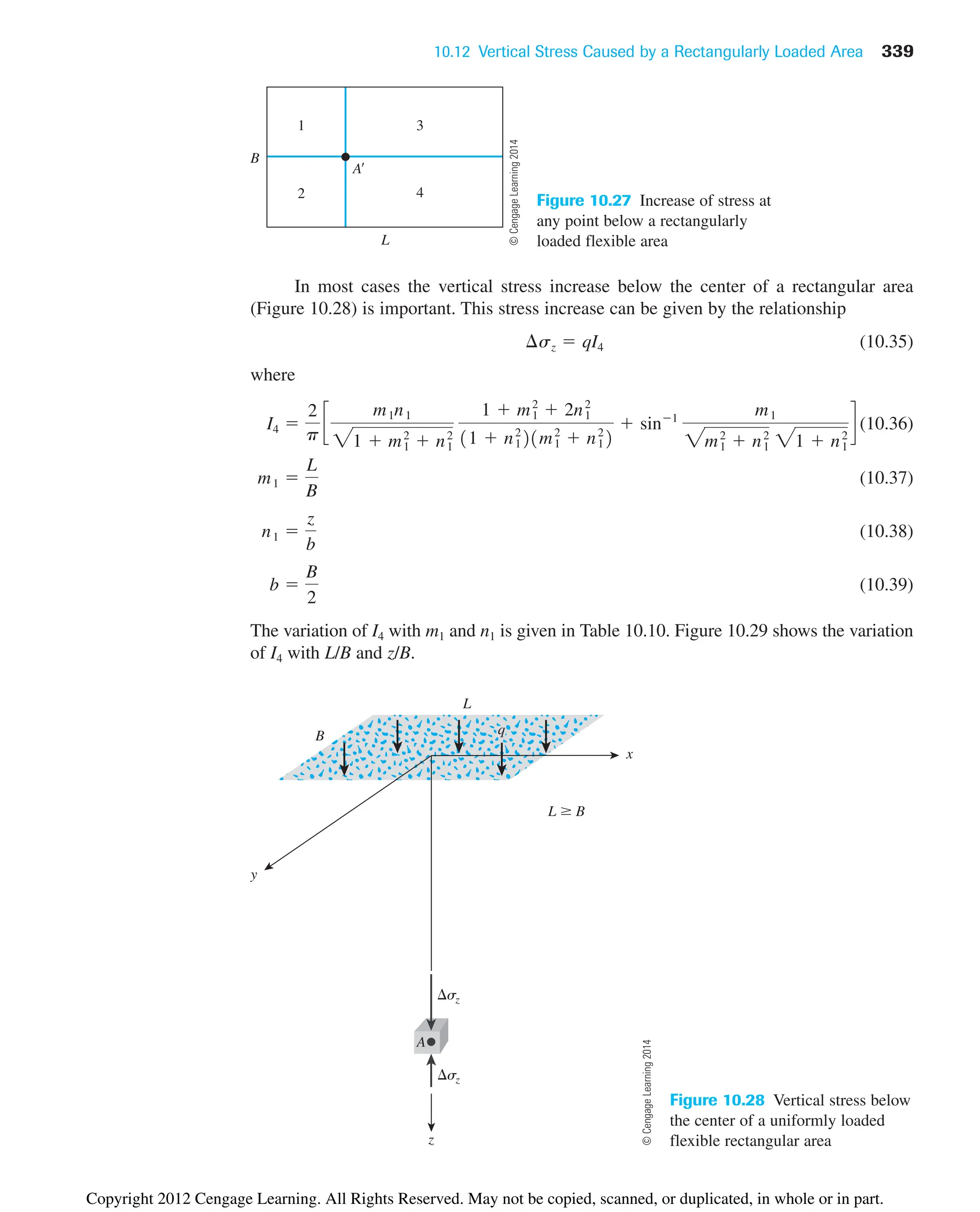
![10.12 Vertical Stress Caused by a Rectangularly Loaded Area 337
Table 10.9 Variation of I3 with m and n [Eq. (10.31)]
m
n 0.1 0.2 0.3 0.4 0.5 0.6 0.7 0.8 0.9 1.0
0.1 0.0047 0.0092 0.0132 0.0168 0.0198 0.0222 0.0242 0.0258 0.0270 0.0279
0.2 0.0092 0.0179 0.0259 0.0328 0.0387 0.0435 0.0474 0.0504 0.0528 0.0547
0.3 0.0132 0.0259 0.0374 0.0474 0.0559 0.0629 0.0686 0.0731 0.0766 0.0794
0.4 0.0168 0.0328 0.0474 0.0602 0.0711 0.0801 0.0873 0.0931 0.0977 0.1013
0.5 0.0198 0.0387 0.0559 0.0711 0.0840 0.0947 0.1034 0.1104 0.1158 0.1202
0.6 0.0222 0.0435 0.0629 0.0801 0.0947 0.1069 0.1168 0.1247 0.1311 0.1361
0.7 0.0242 0.0474 0.0686 0.0873 0.1034 0.1169 0.1277 0.1365 0.1436 0.1491
0.8 0.0258 0.0504 0.0731 0.0931 0.1104 0.1247 0.1365 0.1461 0.1537 0.1598
0.9 0.0270 0.0528 0.0766 0.0977 0.1158 0.1311 0.1436 0.1537 0.1619 0.1684
1.0 0.0279 0.0547 0.0794 0.1013 0.1202 0.1361 0.1491 0.1598 0.1684 0.1752
1.2 0.0293 0.0573 0.0832 0.1063 0.1263 0.1431 0.1570 0.1684 0.1777 0.1851
1.4 0.0301 0.0589 0.0856 0.1094 0.1300 0.1475 0.1620 0.1739 0.1836 0.1914
1.6 0.0306 0.0599 0.0871 0.1114 0.1324 0.1503 0.1652 0.1774 0.1874 0.1955
1.8 0.0309 0.0606 0.0880 0.1126 0.1340 0.1521 0.1672 0.1797 0.1899 0.1981
2.0 0.0311 0.0610 0.0887 0.1134 0.1350 0.1533 0.1686 0.1812 0.1915 0.1999
2.5 0.0314 0.0616 0.0895 0.1145 0.1363 0.1548 0.1704 0.1832 0.1938 0.2024
3.0 0.0315 0.0618 0.0898 0.1150 0.1368 0.1555 0.1711 0.1841 0.1947 0.2034
4.0 0.0316 0.0619 0.0901 0.1153 0.1372 0.1560 0.1717 0.1847 0.1954 0.2042
5.0 0.0316 0.0620 0.0901 0.1154 0.1374 0.1561 0.1719 0.1849 0.1956 0.2044
6.0 0.0316 0.0620 0.0902 0.1154 0.1374 0.1562 0.1719 0.1850 0.1957 0.2045
1.2 1.4 1.6 1.8 2.0 2.5 3.0 4.0 5.0 6.0
0.0293 0.0301 0.0306 0.0309 0.0311 0.0314 0.0315 0.0316 0.0316 0.0316
0.0573 0.0589 0.0599 0.0606 0.0610 0.0616 0.0618 0.0619 0.0620 0.0620
0.0832 0.0856 0.0871 0.0880 0.0887 0.0895 0.0898 0.0901 0.0901 0.0902
0.1063 0.1094 0.1114 0.1126 0.1134 0.1145 0.1150 0.1153 0.1154 0.1154
0.1263 0.1300 0.1324 0.1340 0.1350 0.1363 0.1368 0.1372 0.1374 0.1374
0.1431 0.1475 0.1503 0.1521 0.1533 0.1548 0.1555 0.1560 0.1561 0.1562
0.1570 0.1620 0.1652 0.1672 0.1686 0.1704 0.1711 0.1717 0.1719 0.1719
0.1684 0.1739 0.1774 0.1797 0.1812 0.1832 0.1841 0.1847 0.1849 0.1850
0.1777 0.1836 0.1874 0.1899 0.1915 0.1938 0.1947 0.1954 0.1956 0.1957
0.1851 0.1914 0.1955 0.1981 0.1999 0.2024 0.2034 0.2042 0.2044 0.2045
0.1958 0.2028 0.2073 0.2103 0.2124 0.2151 0.2163 0.2172 0.2175 0.2176
0.2028 0.2102 0.2151 0.2184 0.2206 0.2236 0.2250 0.2260 0.2263 0.2264
0.2073 0.2151 0.2203 0.2237 0.2261 0.2294 0.2309 0.2320 0.2323 0.2325
0.2103 0.2183 0.2237 0.2274 0.2299 0.2333 0.2350 0.2362 0.2366 0.2367
0.2124 0.2206 0.2261 0.2299 0.2325 0.2361 0.2378 0.2391 0.2395 0.2397
0.2151 0.2236 0.2294 0.2333 0.2361 0.2401 0.2420 0.2434 0.2439 0.2441
0.2163 0.2250 0.2309 0.2350 0.2378 0.2420 0.2439 0.2455 0.2461 0.2463
0.2172 0.2260 0.2320 0.2362 0.2391 0.2434 0.2455 0.2472 0.2479 0.2481
0.2175 0.2263 0.2324 0.2366 0.2395 0.2439 0.2460 0.2479 0.2486 0.2489
0.2176 0.2264 0.2325 0.2367 0.2397 0.2441 0.2463 0.2482 0.2489 0.2492
©
Cengage
Learning
2014
Copyright 2012 Cengage Learning. All Rights Reserved. May not be copied, scanned, or duplicated, in whole or in part.](https://image.slidesharecdn.com/principlesofgeotechnicalengineering-8thedition-231222125509-7e44d9bf/75/Principles-of-Geotechnical-Engineering-8th-Edition-pdf-357-2048.jpg)
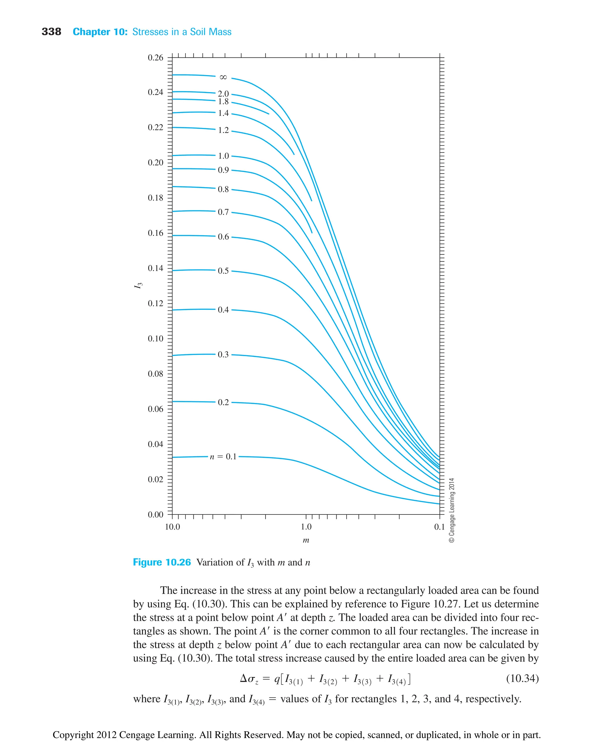
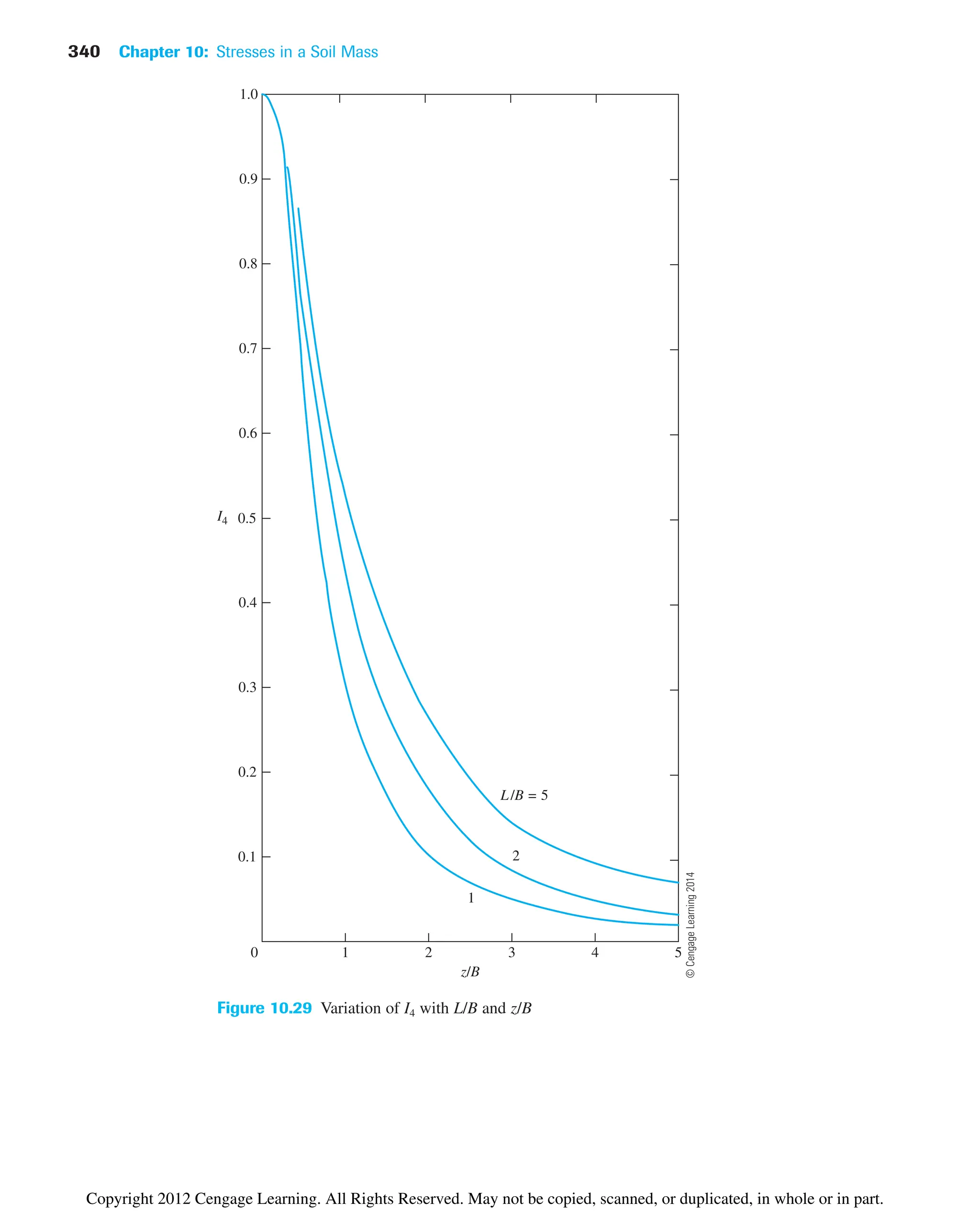
![10.12 Vertical Stress Caused by a Rectangularly Loaded Area 341
Table 10.10 Variation of I4 with m1 and n1 [Eq. (10.36)]
m1
n1 1 2 3 4 5 6 7 8 9 10
0.20 0.994 0.997 0.997 0.997 0.997 0.997 0.997 0.997 0.997 0.997
0.40 0.960 0.976 0.977 0.977 0.977 0.977 0.977 0.977 0.977 0.977
0.60 0.892 0.932 0.936 0.936 0.937 0.937 0.937 0.937 0.937 0.937
0.80 0.800 0.870 0.878 0.880 0.881 0.881 0.881 0.881 0.881 0.881
1.00 0.701 0.800 0.814 0.817 0.818 0.818 0.818 0.818 0.818 0.818
1.20 0.606 0.727 0.748 0.753 0.754 0.755 0.755 0.755 0.755 0.755
1.40 0.522 0.658 0.685 0.692 0.694 0.695 0.695 0.696 0.696 0.696
1.60 0.449 0.593 0.627 0.636 0.639 0.640 0.641 0.641 0.641 0.642
1.80 0.388 0.534 0.573 0.585 0.590 0.591 0.592 0.592 0.593 0.593
2.00 0.336 0.481 0.525 0.540 0.545 0.547 0.548 0.549 0.549 0.549
3.00 0.179 0.293 0.348 0.373 0.384 0.389 0.392 0.393 0.394 0.395
4.00 0.108 0.190 0.241 0.269 0.285 0.293 0.298 0.301 0.302 0.303
5.00 0.072 0.131 0.174 0.202 0.219 0.229 0.236 0.240 0.242 0.244
6.00 0.051 0.095 0.130 0.155 0.172 0.184 0.192 0.197 0.200 0.202
7.00 0.038 0.072 0.100 0.122 0.139 0.150 0.158 0.164 0.168 0.171
8.00 0.029 0.056 0.079 0.098 0.113 0.125 0.133 0.139 0.144 0.147
9.00 0.023 0.045 0.064 0.081 0.094 0.105 0.113 0.119 0.124 0.128
10.00 0.019 0.037 0.053 0.067 0.079 0.089 0.097 0.103 0.108 0.112
Example 10.10
The plan of a uniformly loaded rectangular area is shown in Figure 10.30a. Determine
the vertical stress increase below point at a depth of z 4 m.
A¿
¢sz
q 150 kN/m2
q
150
kN/m2
A A
4 m
1 m
1 m
2 m
q 150 kN/m2
A
3 m
2 m
2 m
(a)
(b) (c)
Figure 10.30
©
Cengage
Learning
2014
©
Cengage
Learning
2014
Copyright 2012 Cengage Learning. All Rights Reserved. May not be copied, scanned, or duplicated, in whole or in part.](https://image.slidesharecdn.com/principlesofgeotechnicalengineering-8thedition-231222125509-7e44d9bf/75/Principles-of-Geotechnical-Engineering-8th-Edition-pdf-361-2048.jpg)
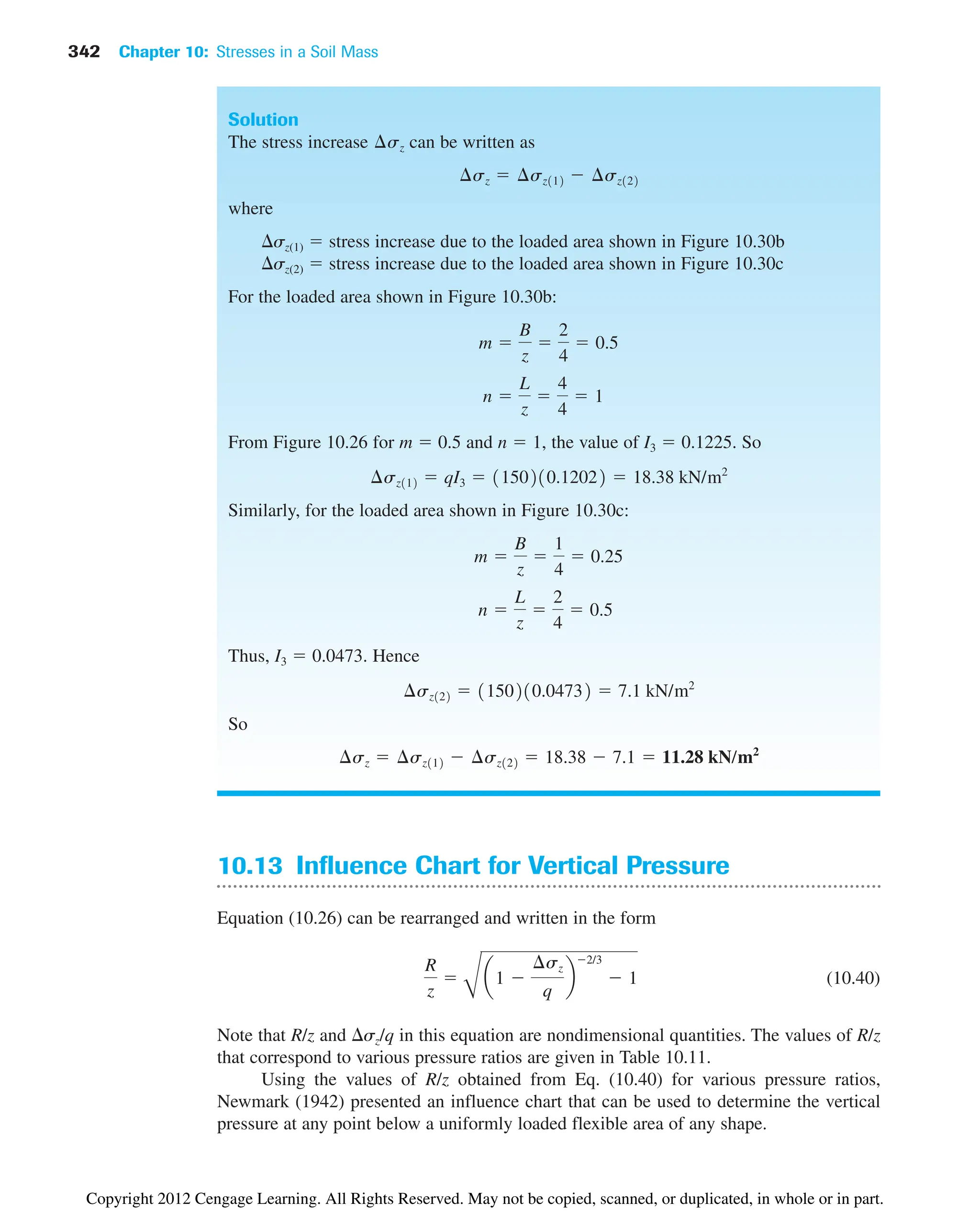
![10.13 Influence Chart for Vertical Pressure 343
Table 10.11 Values of R/z for Various Pressure Ratios [Eq. (10.40)]
sz /q R/z sz /q R/z
0 0 0.55 0.8384
0.05 0.1865 0.60 0.9176
0.10 0.2698 0.65 1.0067
0.15 0.3383 0.70 1.1097
0.20 0.4005 0.75 1.2328
0.25 0.4598 0.80 1.3871
0.30 0.5181 0.85 1.5943
0.35 0.5768 0.90 1.9084
0.40 0.6370 0.95 2.5232
0.45 0.6997 1.00 q
0.50 0.7664
Influence
value 0.005
A B
Figure 10.31 Influence chart for vertical
pressure based on Boussinesq’s theory
(Bulletin No. 338. Influence Charts for
Computation of Stresses in Elastic.
Foundations, by Nathan M. Newmark.
University of Illinois, 1942.)
Figure 10.31 shows an influence chart that has been constructed by drawing con-
centric circles. The radii of the circles are equal to the R/z values corresponding to
sz/q 0, 0.1, 0.2, . . . , 1. (Note: For sz/q 0, R/z 0, and for sz/q 1, R/z `,
so nine circles are shown.) The unit length for plotting the circles is . The circles are
divided by several equally spaced radial lines. The influence value of the chart is given
by 1/N, where N is equal to the number of elements in the chart. In Figure 10.31, there
are 200 elements; hence, the influence value is 0.005.
AB
©
Cengage
Learning
2014
Copyright 2012 Cengage Learning. All Rights Reserved. May not be copied, scanned, or duplicated, in whole or in part.](https://image.slidesharecdn.com/principlesofgeotechnicalengineering-8thedition-231222125509-7e44d9bf/75/Principles-of-Geotechnical-Engineering-8th-Edition-pdf-363-2048.jpg)
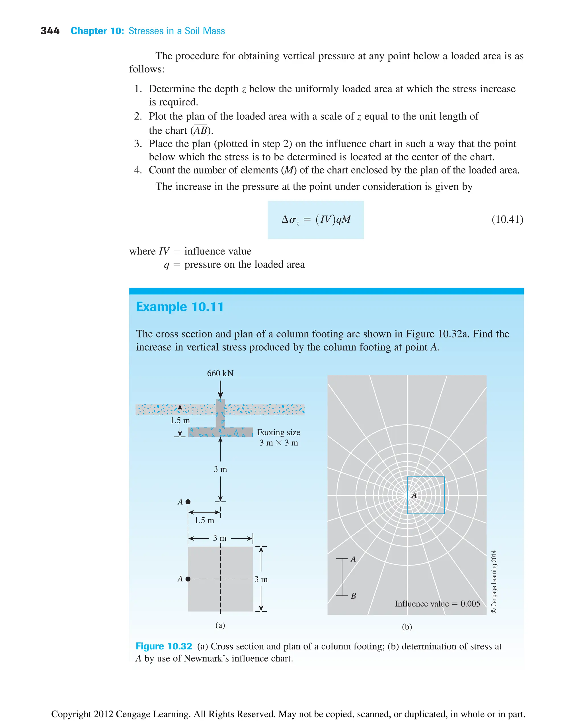
![10.14 Summary and General Comments 345
Solution
Point A is located at à depth 3 m below the bottom of the footing. The plan of the square
footing has been replotted to a scale of 3 m and placed on the influence chart
(Figure 10.32b) in such a way that point A on the plan falls directly over the center of
the chart. The number of elements inside the outline of the plan is about 48.5. Hence,
¢sz 1IV2qM 0.005a
660
3 3
b48.5 17.78 kN/m2
AB
10.14 Summary and General Comments
In this chapter, we have studied the following:
• Determination of the normal and shear stresses on an inclined plane based on the
stress conditions on a two-dimensional soil element [Eqs. (10.3)
and (10.4)].
• The principles of Mohr’s circle and the pole method to determine the stress along a
plane have been provided in Sections 10.2 and 10.3, respectively.
• The vertical stress (sz) produced at any point in a homogeneous, elastic, and
isotropic medium as a result of various types of load applied on the surface of an
infinitely large half-space has been presented. The following table provides a list of
the type of loading and the corresponding relationships to determine vertical stress.
Type of loading Equation number to estimate z
Point load 10.12
Vertical line load 10.16
Horizontal line load 10.17
Vertical strip load 10.19
Linearly increasing vertical load on a strip 10.20
Embankment loading 10.21
Uniformly loaded circular area 10.26, 10.27
Uniformly loaded rectangular area 10.30, 10.35
• The concept of using an influence chart to determine the vertical pressure at any
point below a loaded area is given in Section 10.13.
The equations and graphs presented in this chapter are based entirely on the prin-
ciples of the theory of elasticity; however, one must realize the limitations of these the-
ories when they are applied to a soil medium. This is because soil deposits, in general,
are not homogeneous, perfectly elastic, and isotropic. Hence, some deviations from the
theoretical stress calculations can be expected in the field. Only a limited number of
field observations are available in the literature for comparision purposes. On the basis
of these results, it appears that one could expect a difference of 25 to 30% between
theoretical estimates and actual field values.
©
Cengage
Learning
2014
Copyright 2012 Cengage Learning. All Rights Reserved. May not be copied, scanned, or duplicated, in whole or in part.](https://image.slidesharecdn.com/principlesofgeotechnicalengineering-8thedition-231222125509-7e44d9bf/75/Principles-of-Geotechnical-Engineering-8th-Edition-pdf-365-2048.jpg)
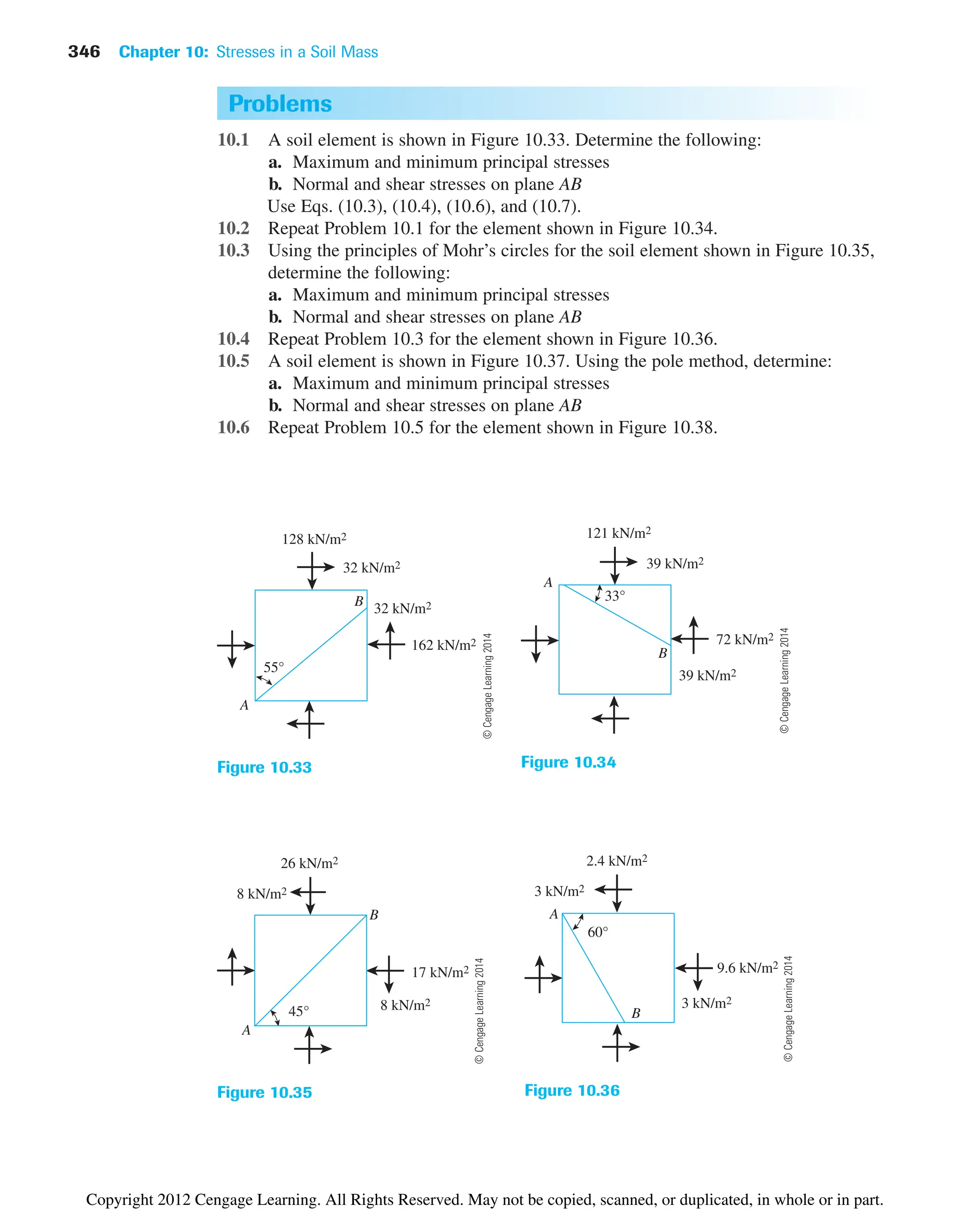
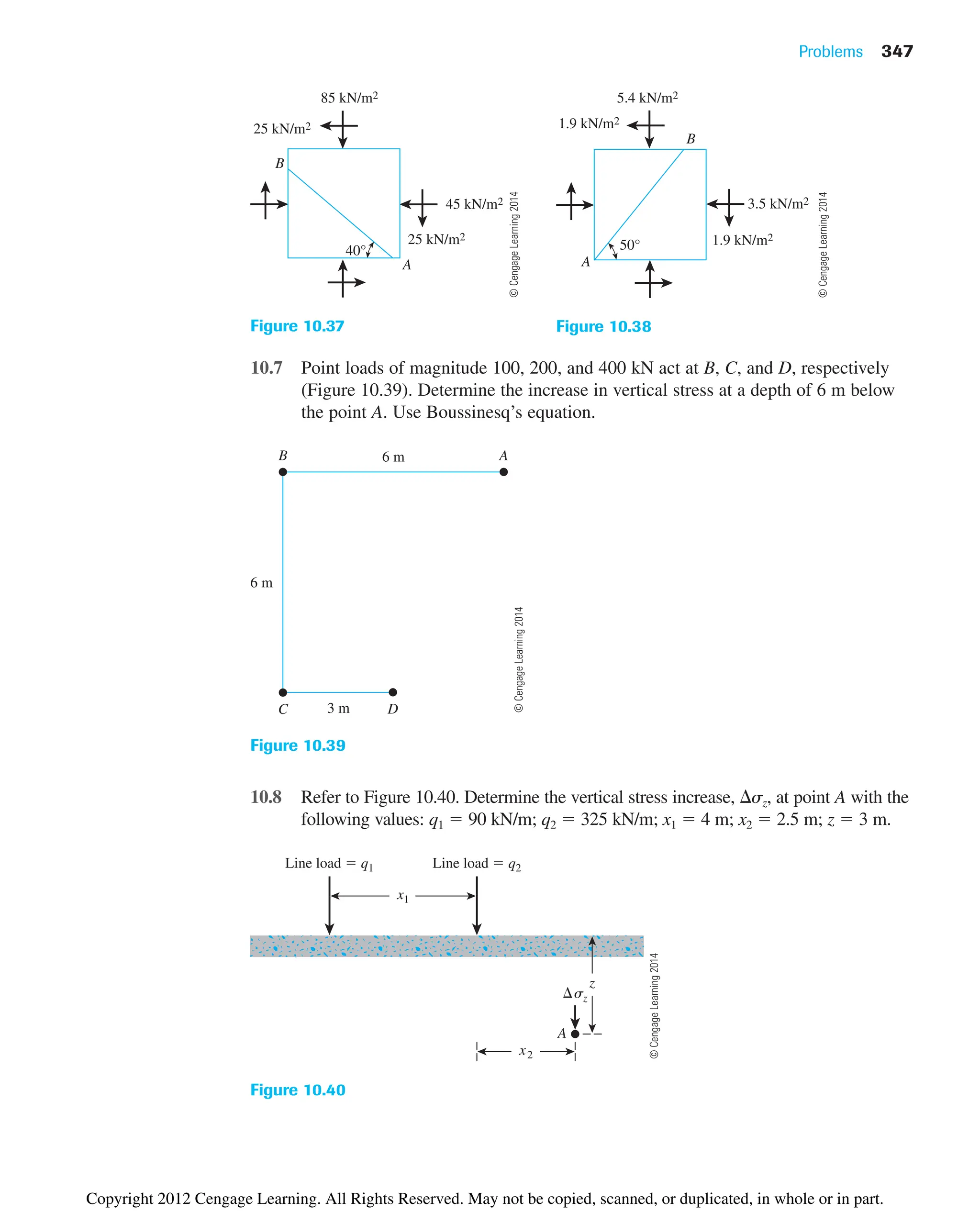
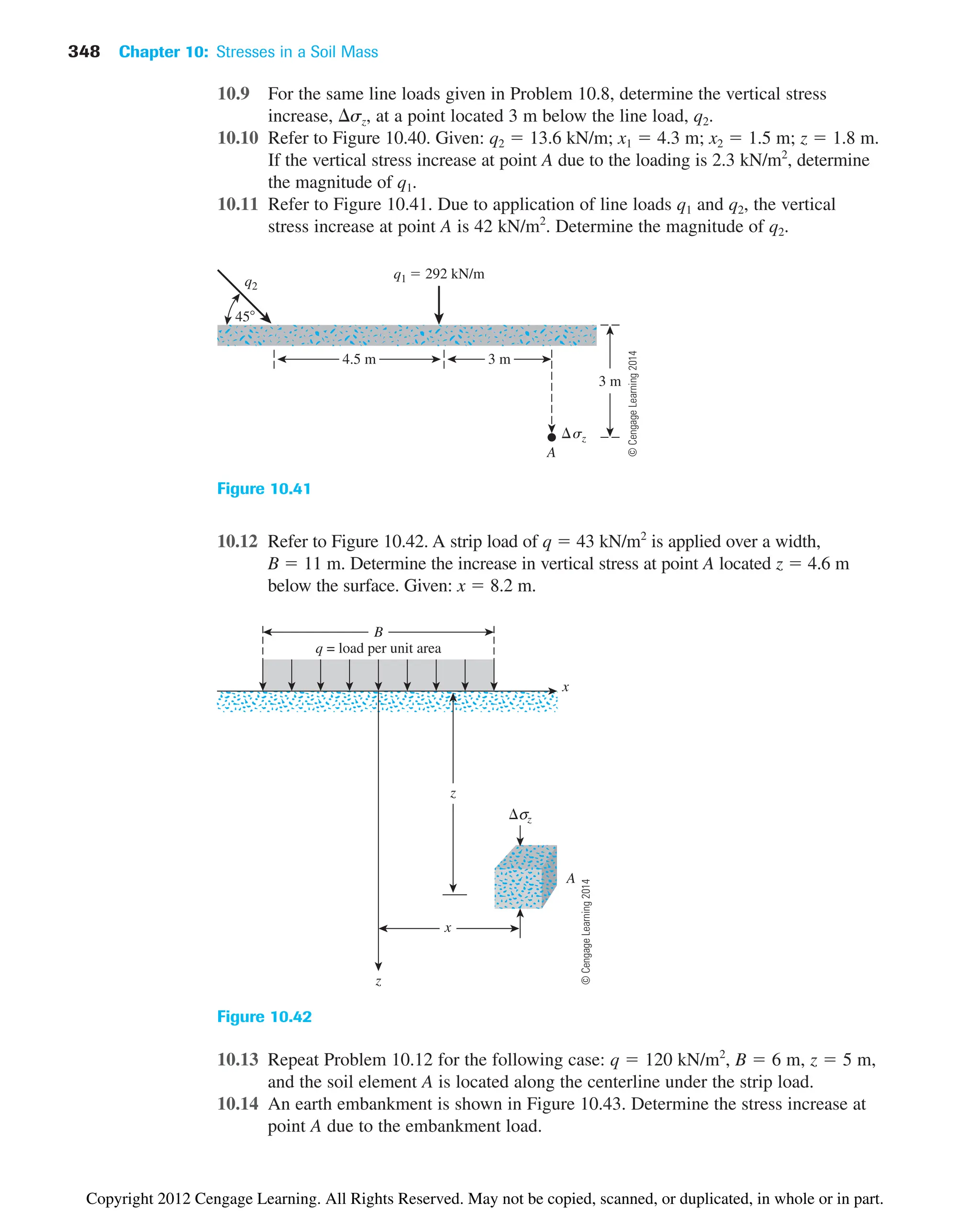
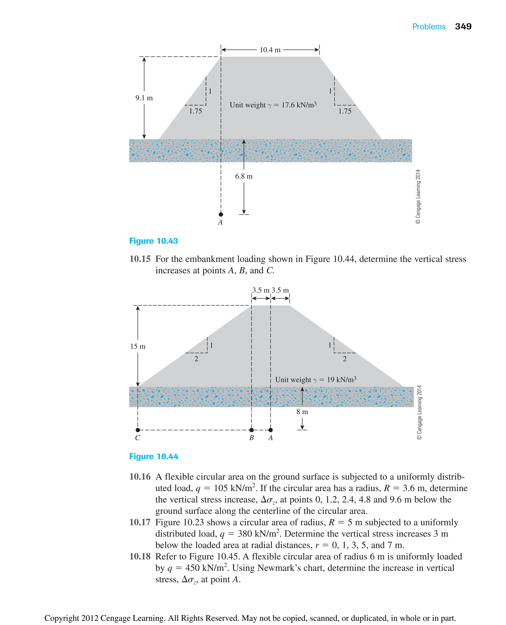
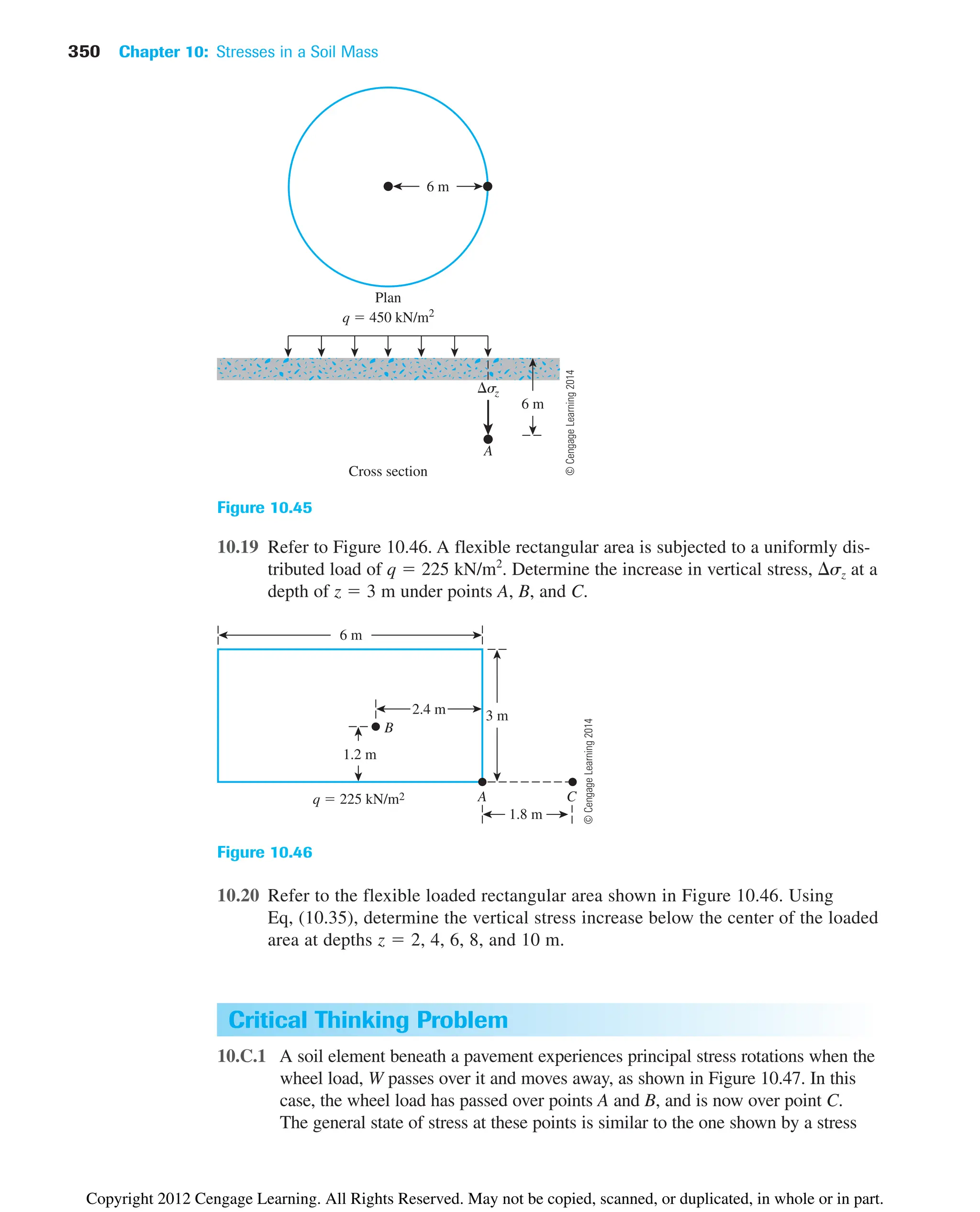
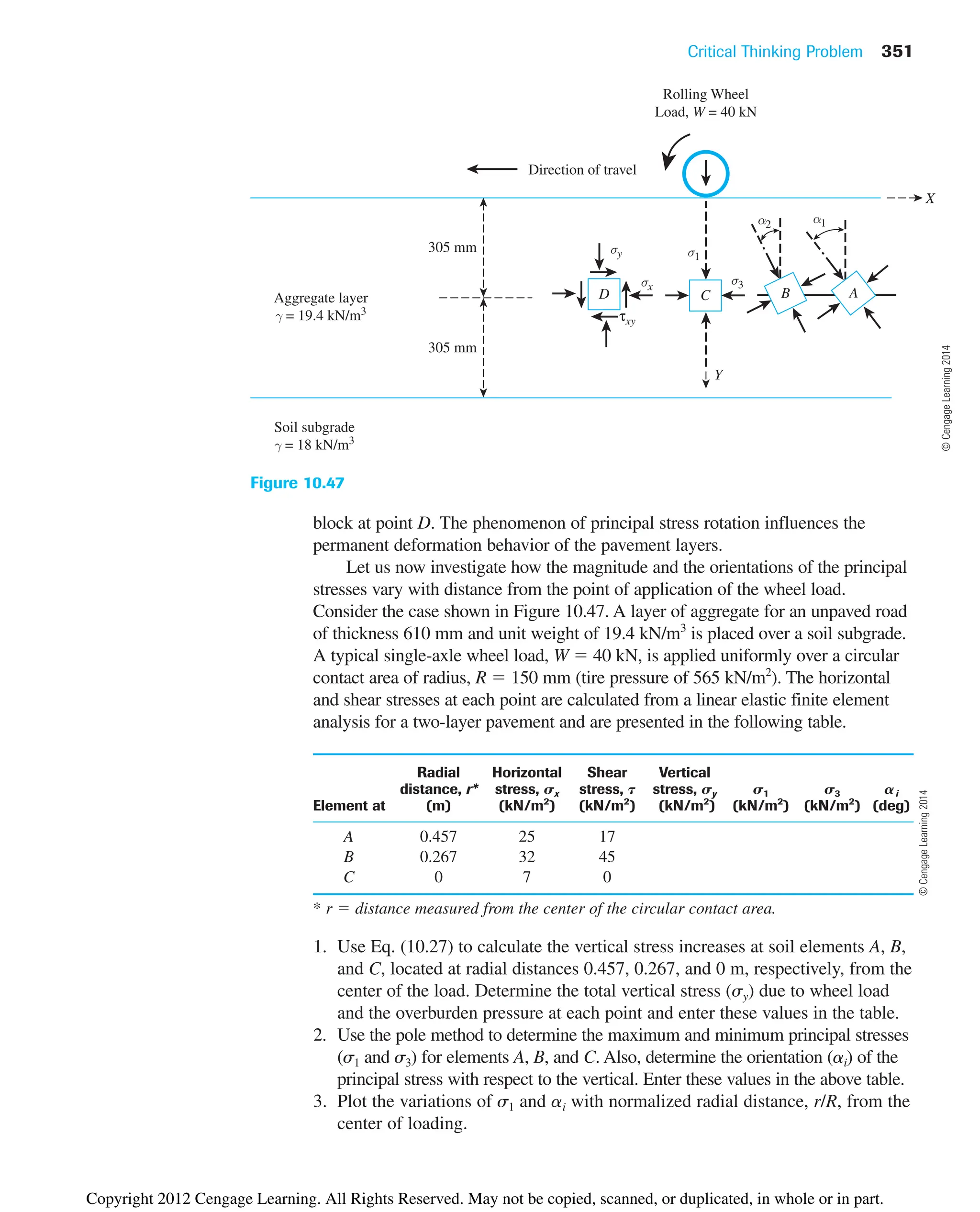
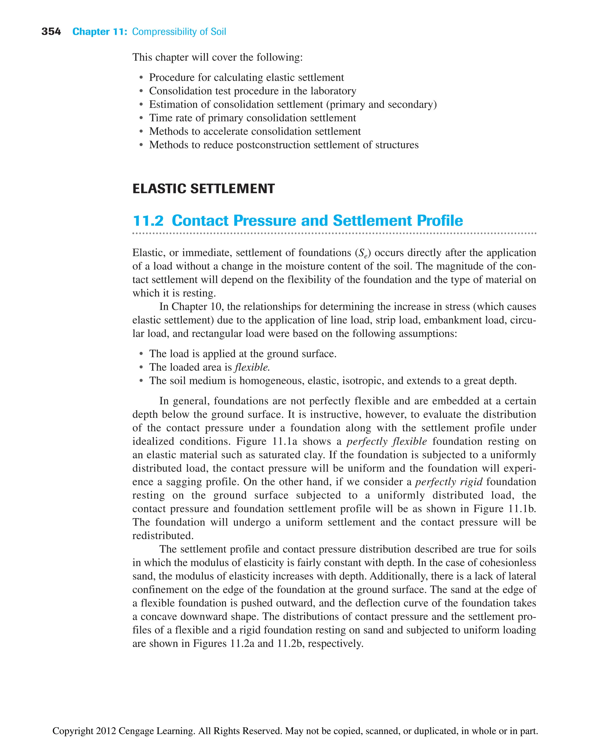
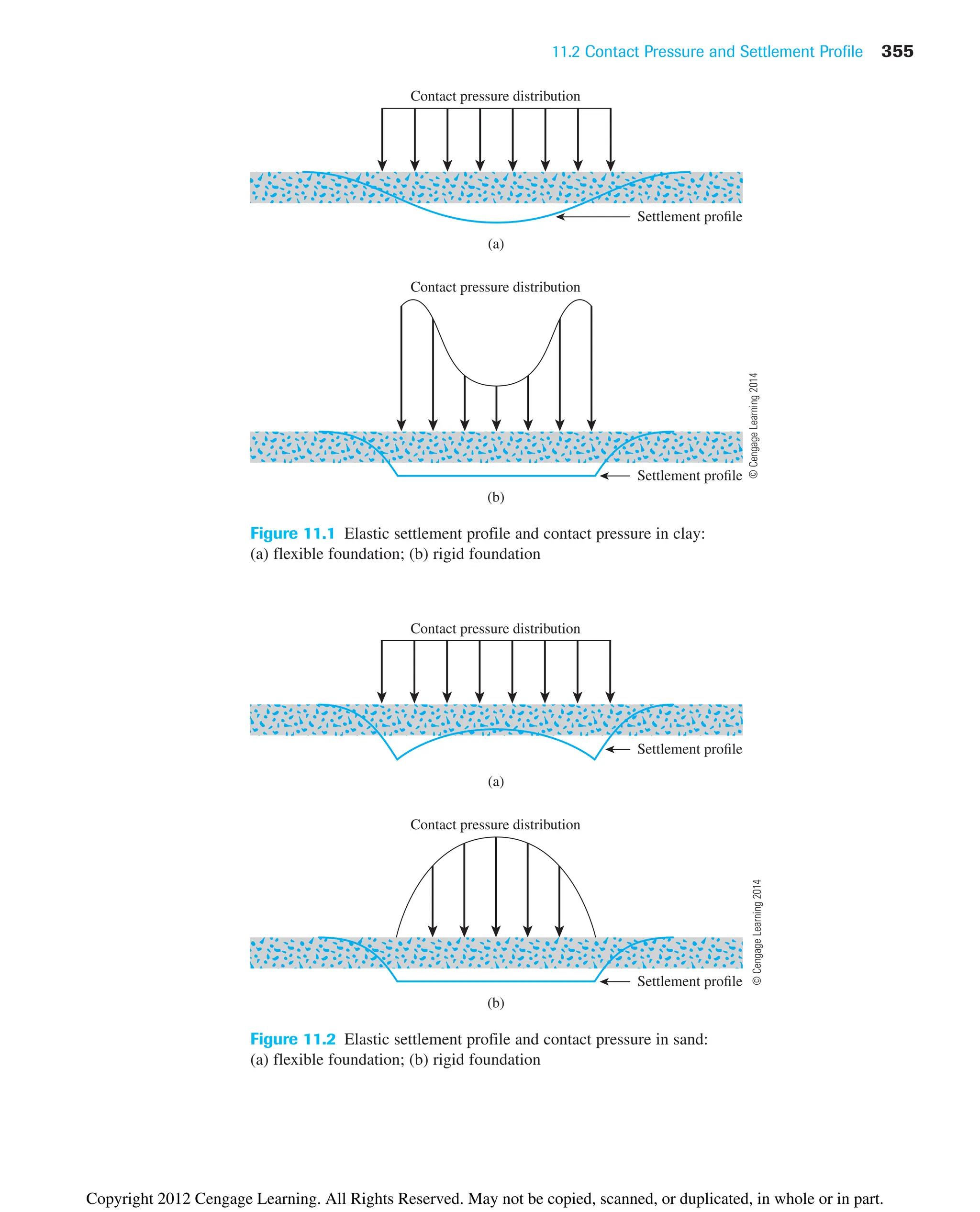
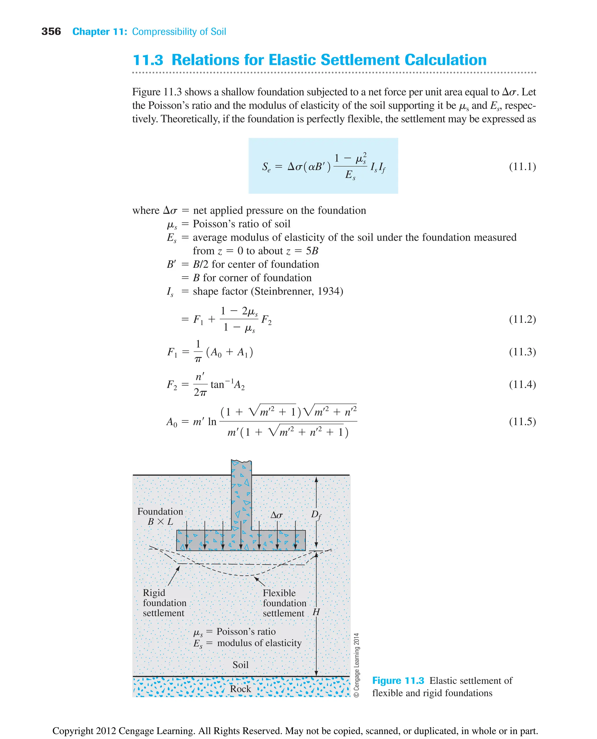
![11.3 Relations for Elastic Settlement Calculation 357
(11.6)
(11.7)
(11.8)
a factor that depends on the location on the foundation where settlement is
being calculated
• For calculation of settlement at the center of the foundation:
• For calculation of settlement at a corner of the foundation:
The variations of F1 and F2 [Eqs. (11.3) and (11.4)] with m¿ and n¿ are given in Tables 11.1
and 11.2. Also the variation of If with Df /B and ms is given in Table 11.3. Note that when
Df 0, the value of If 1 in all cases.
The elastic settlement of a rigid foundation can be estimated as
(11.9)
Due to the nonhomogeneous nature of soil deposits, the magnitude of Es may vary
with depth. For that reason, Bowles (1987) recommended using a weighted average value
of Es in Eq. (11.1) or
(11.10)
where Es(i) soil modulus of elasticity within a depth z
H or 5B, whichever is smaller
Representative values of the modulus of elasticity and Poisson’s ratio for different
types of soils are given in Tables 11.4 and 11.5, respectively.
z
Es
gEs1i2¢z
z
Se1rigid2 ⬇ 0.93Se1flexible, center2
n¿
H
B
m¿
L
B
a 1
n¿
H
a
B
2
b
m¿
L
B
a 4
If depth factor 1Fox, 19482 f a
Df
B
, ms, and
L
B
b
A2
m¿
n¿ 2mœ2
nœ2
1
A1 ln
1m¿ 2mœ2
1221 nœ2
m¿ 2mœ2
nœ2
1
Copyright 2012 Cengage Learning. All Rights Reserved. May not be copied, scanned, or duplicated, in whole or in part.](https://image.slidesharecdn.com/principlesofgeotechnicalengineering-8thedition-231222125509-7e44d9bf/75/Principles-of-Geotechnical-Engineering-8th-Edition-pdf-377-2048.jpg)
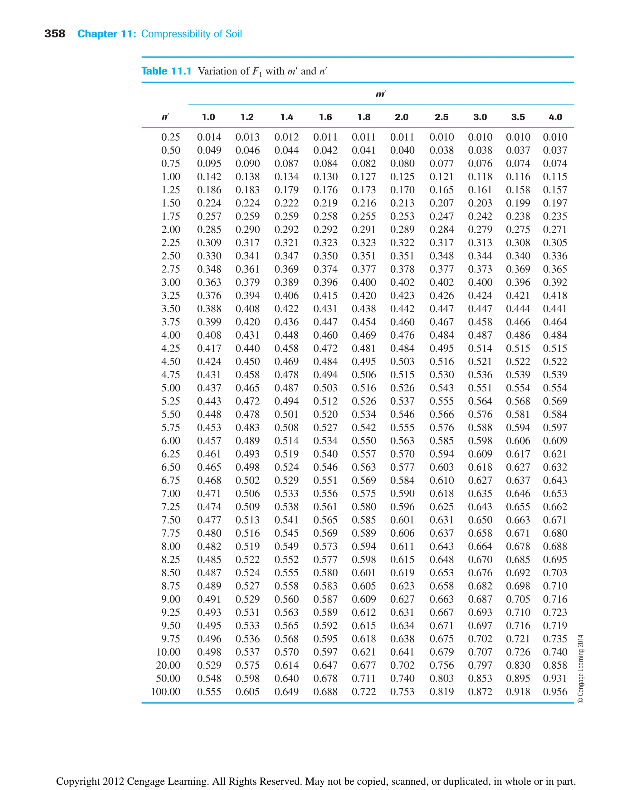
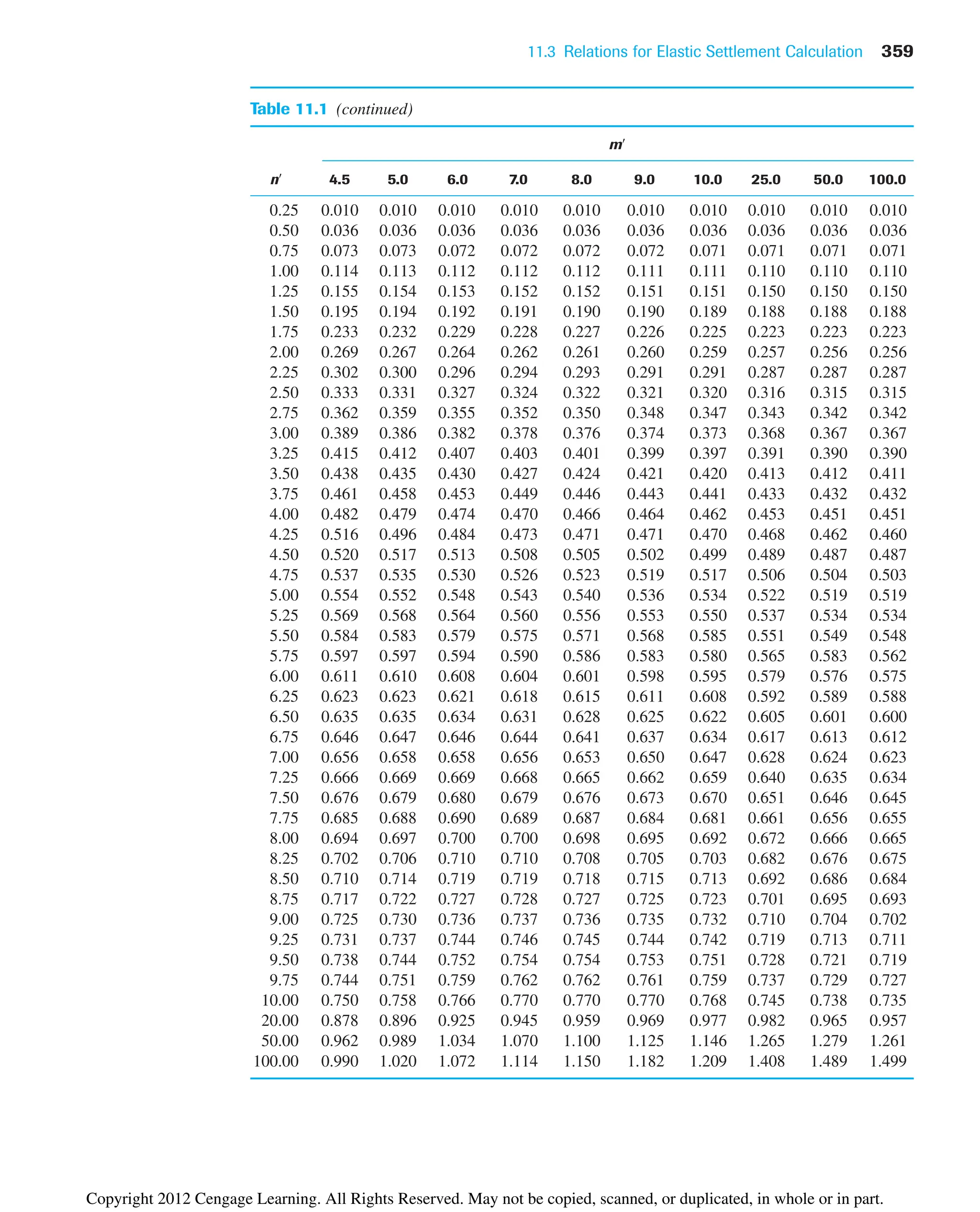
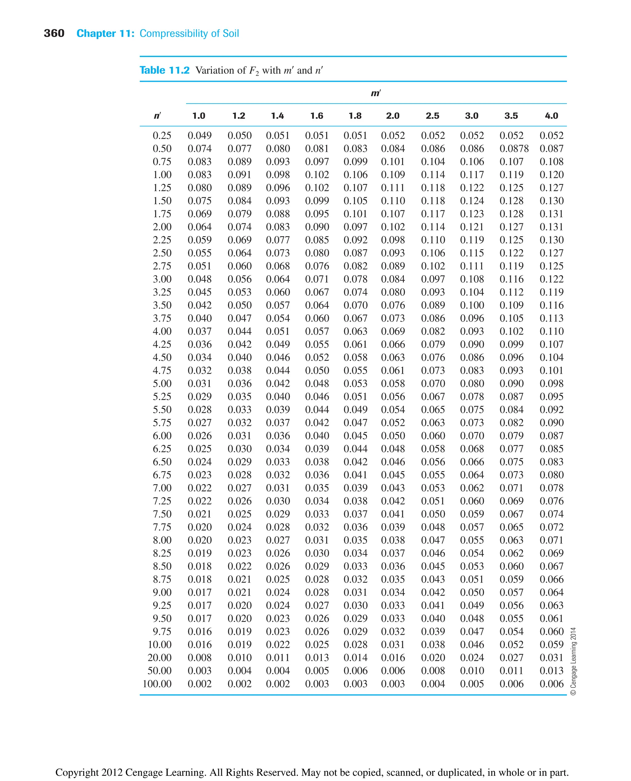
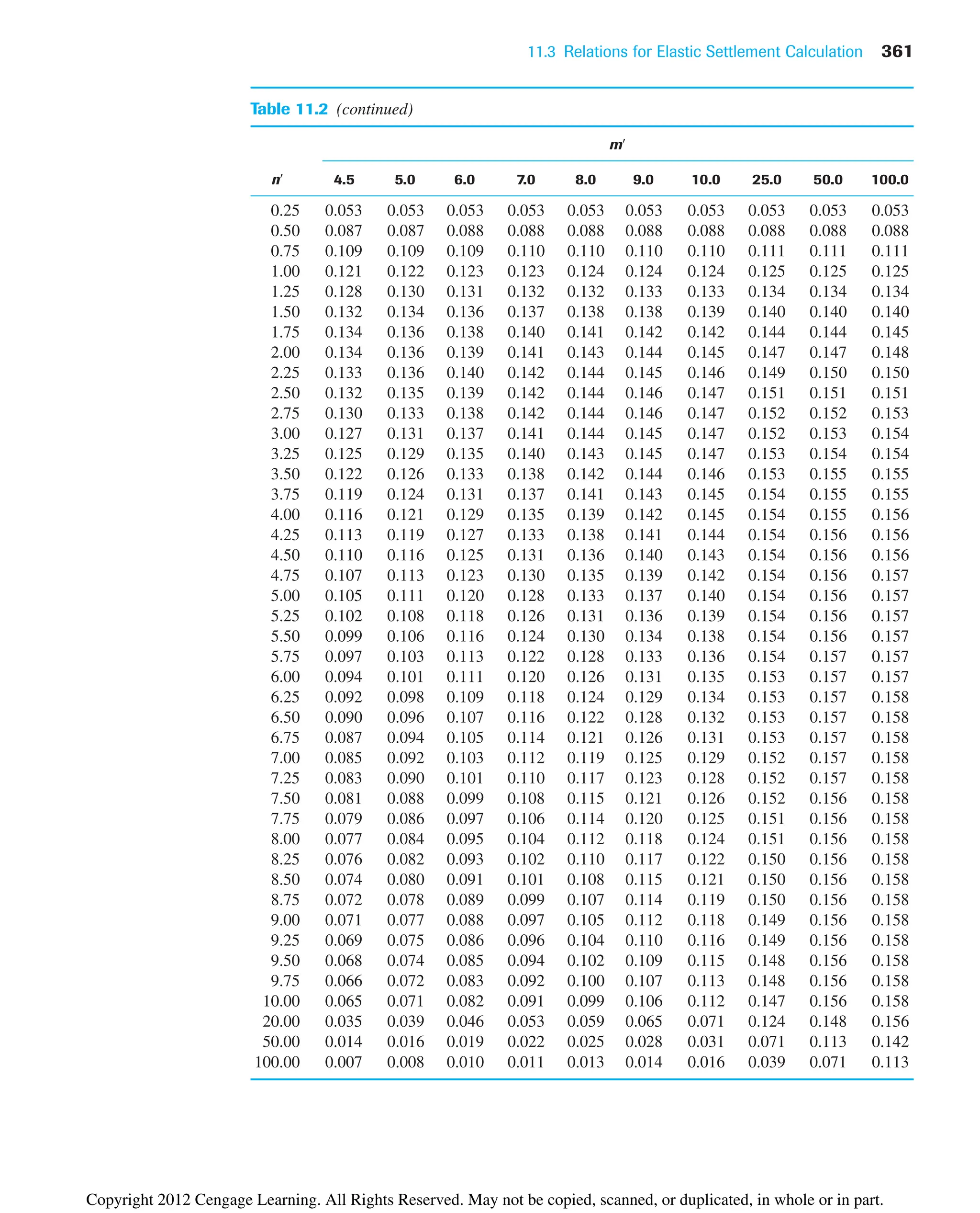
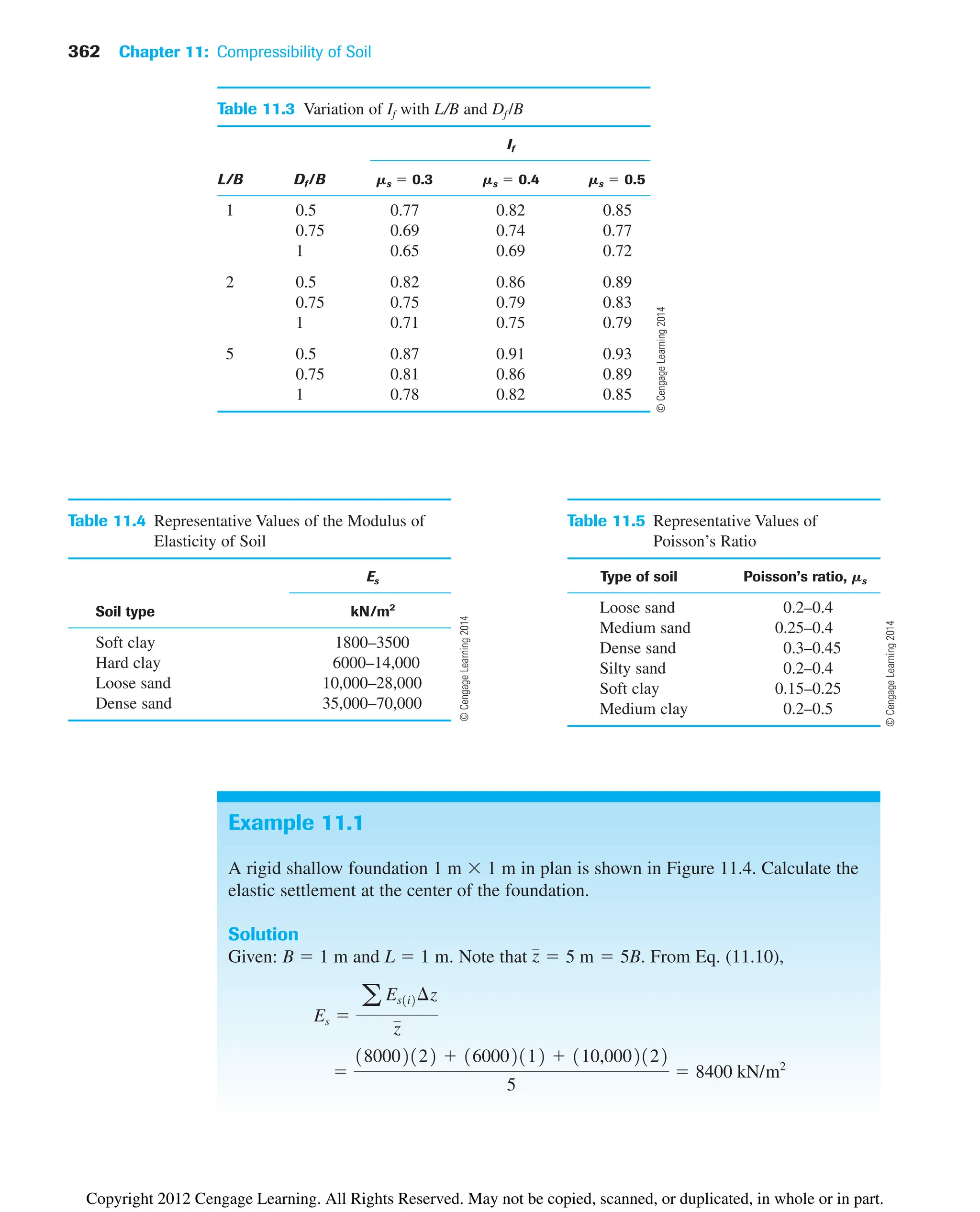
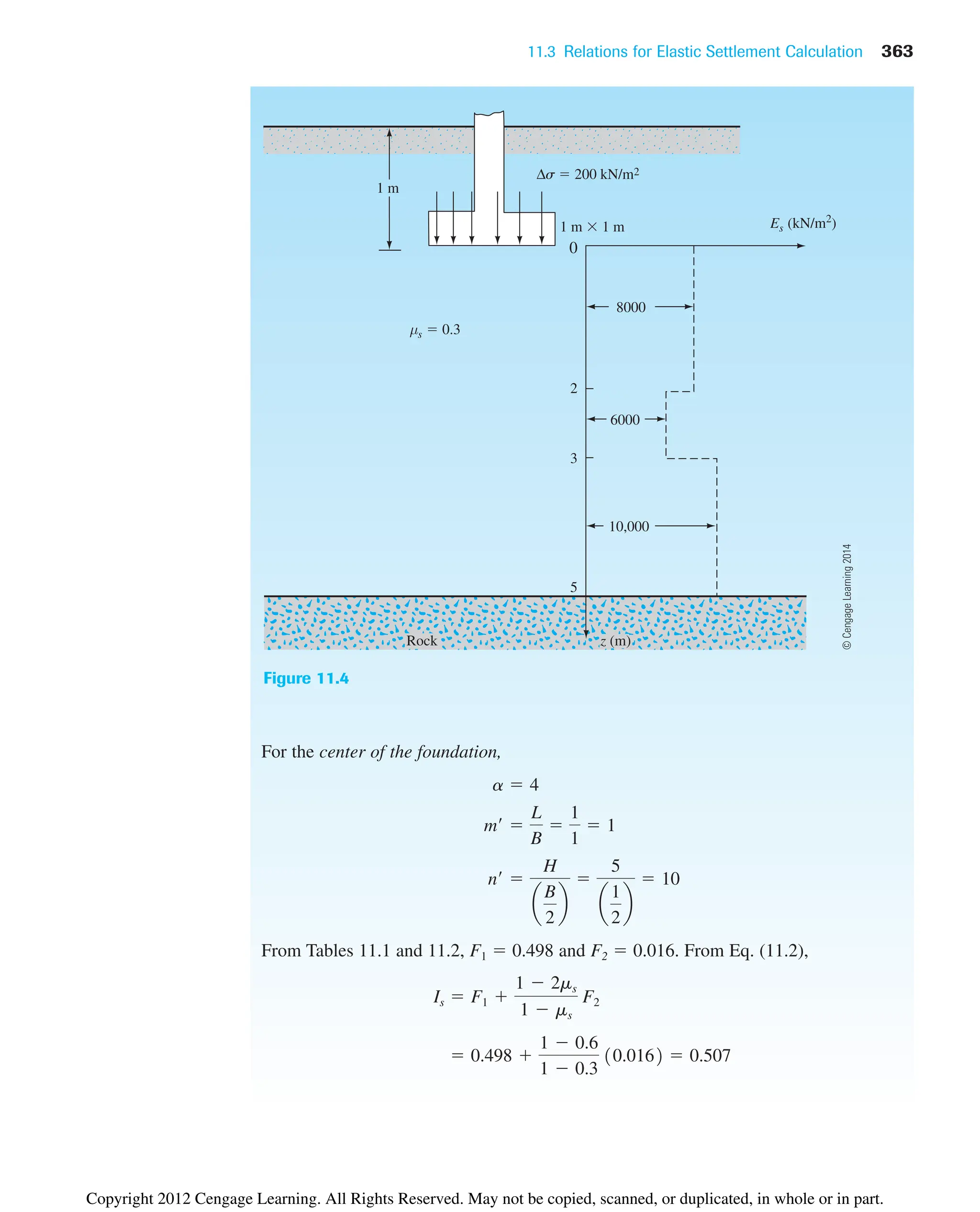
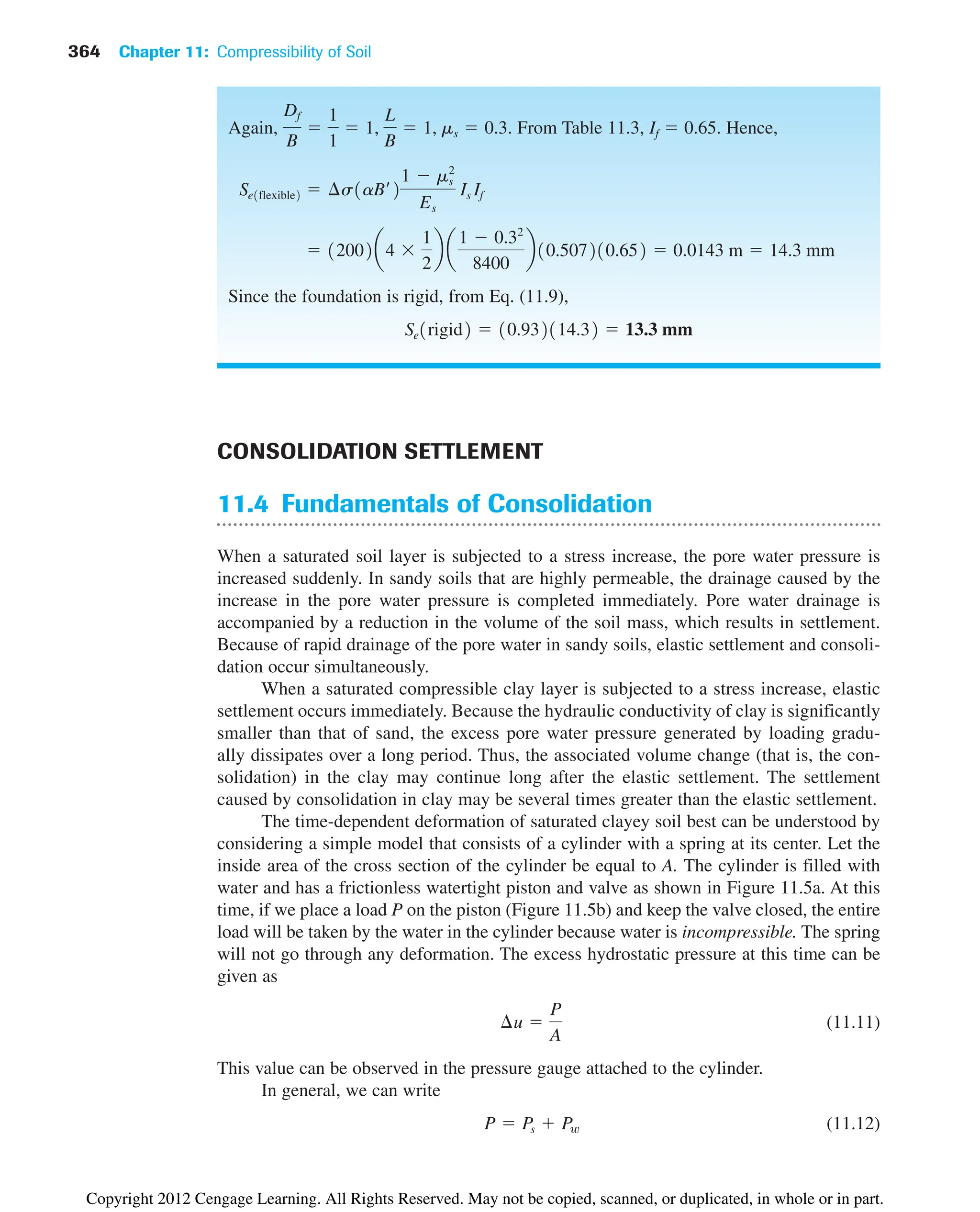
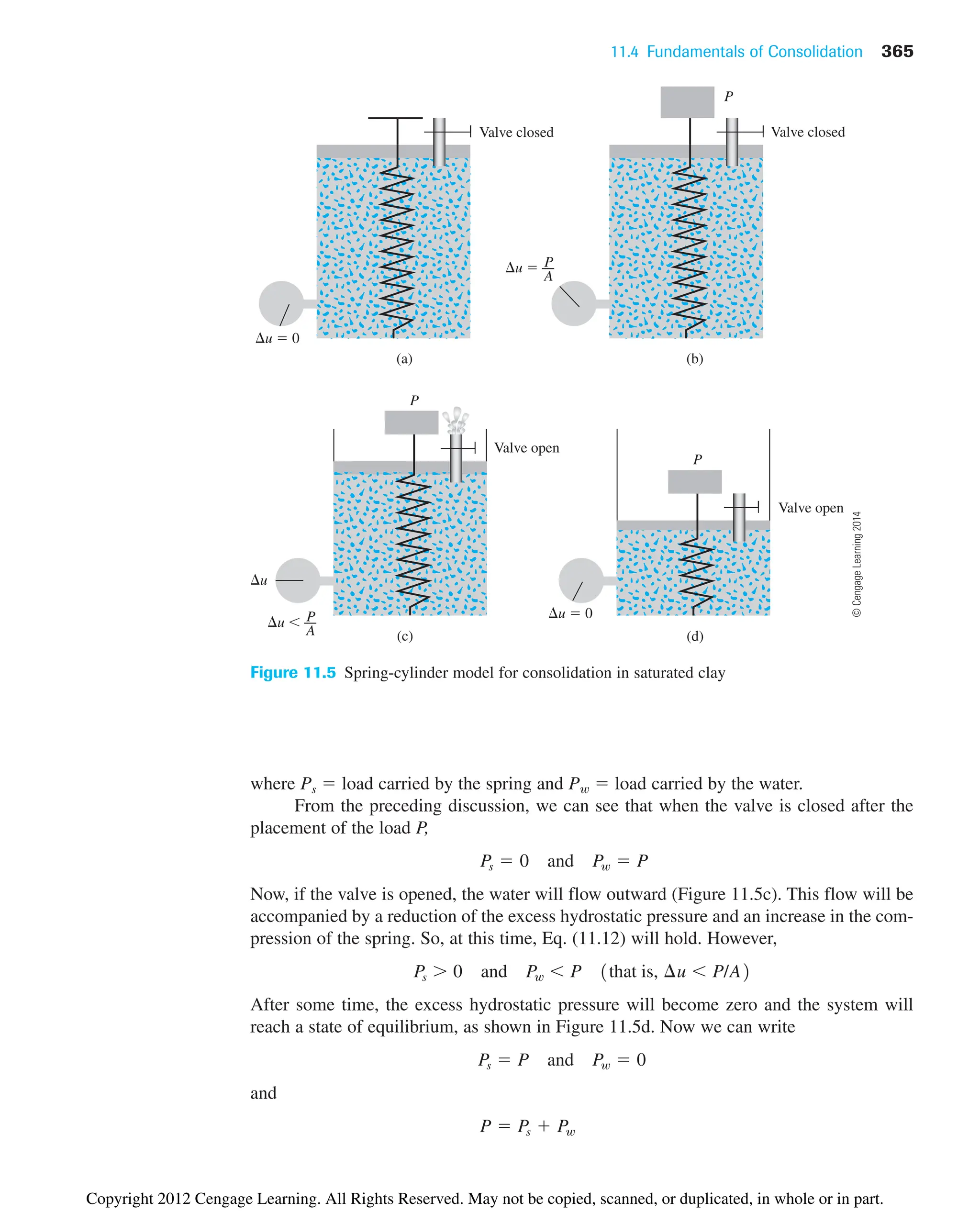
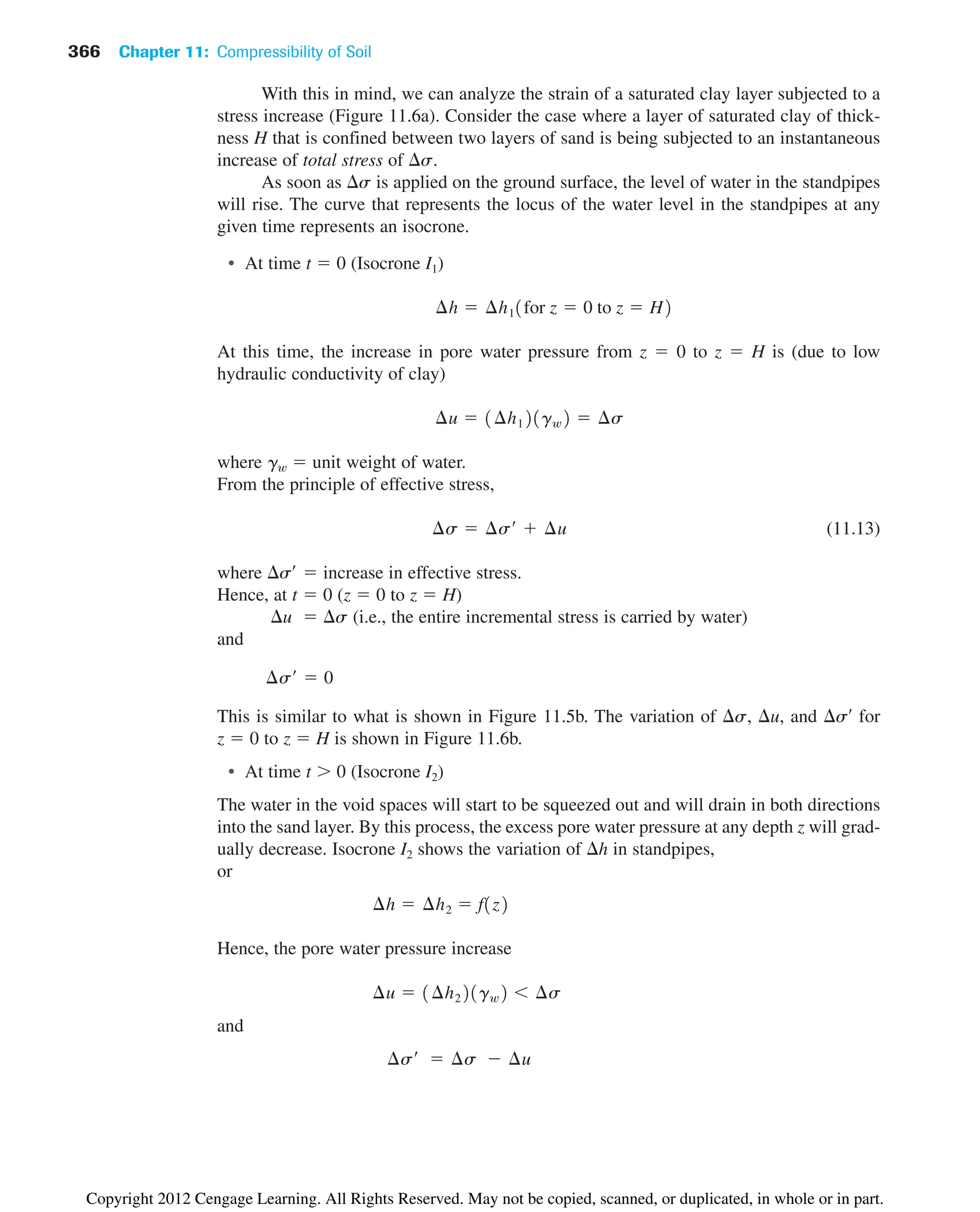
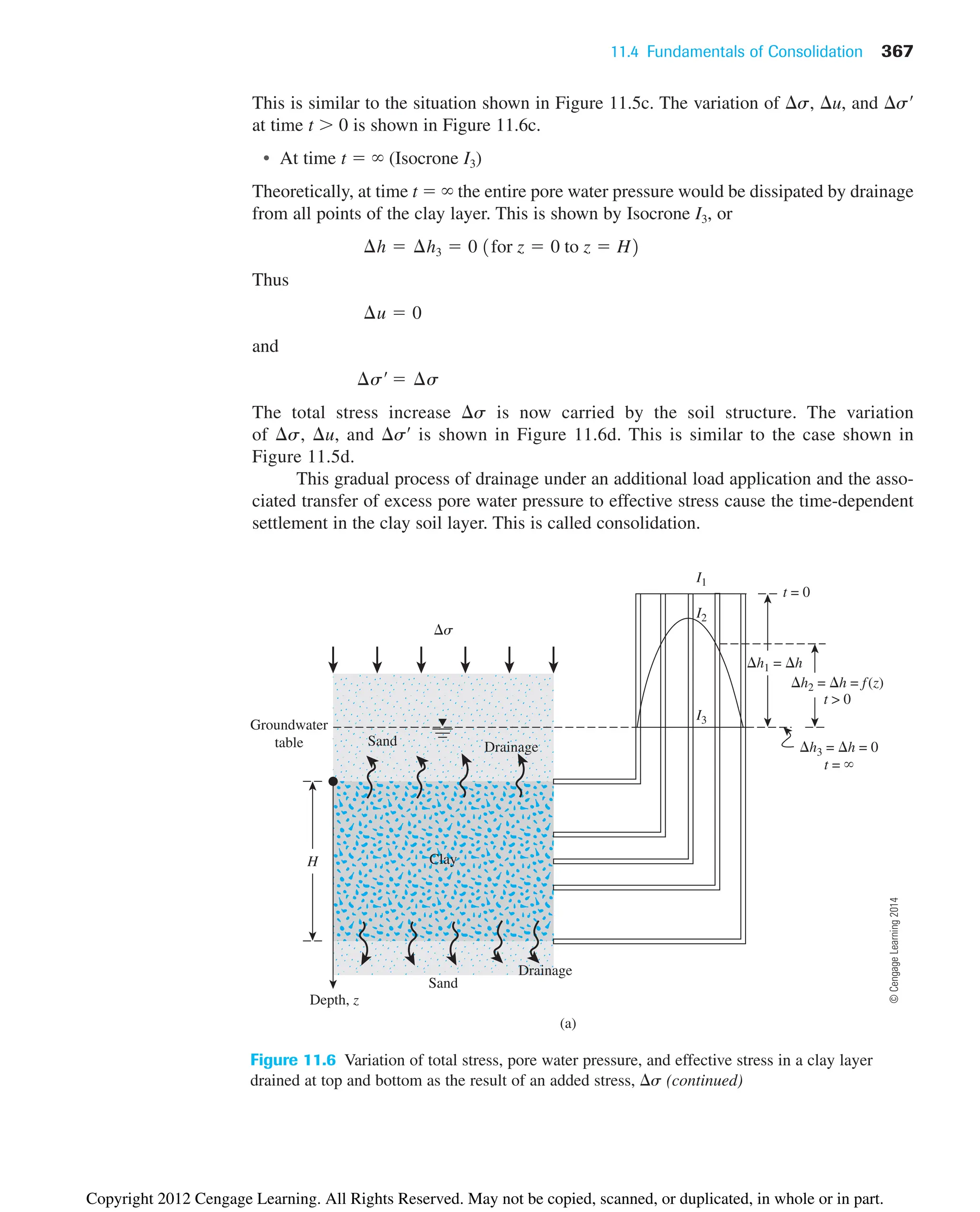
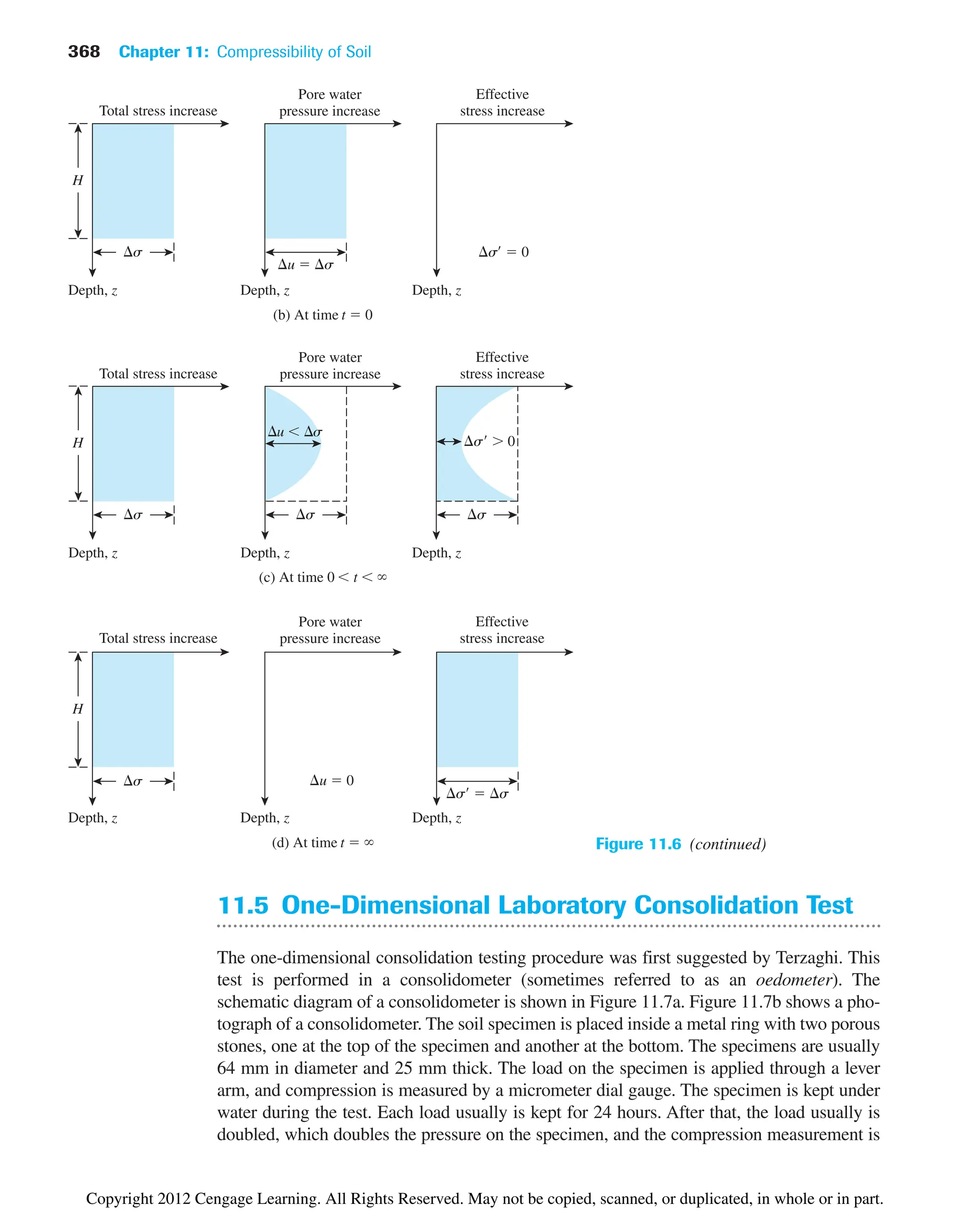
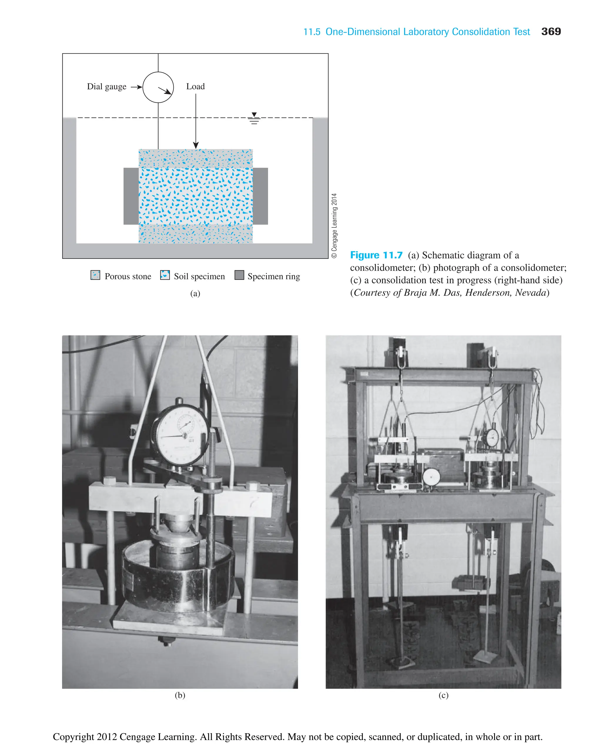
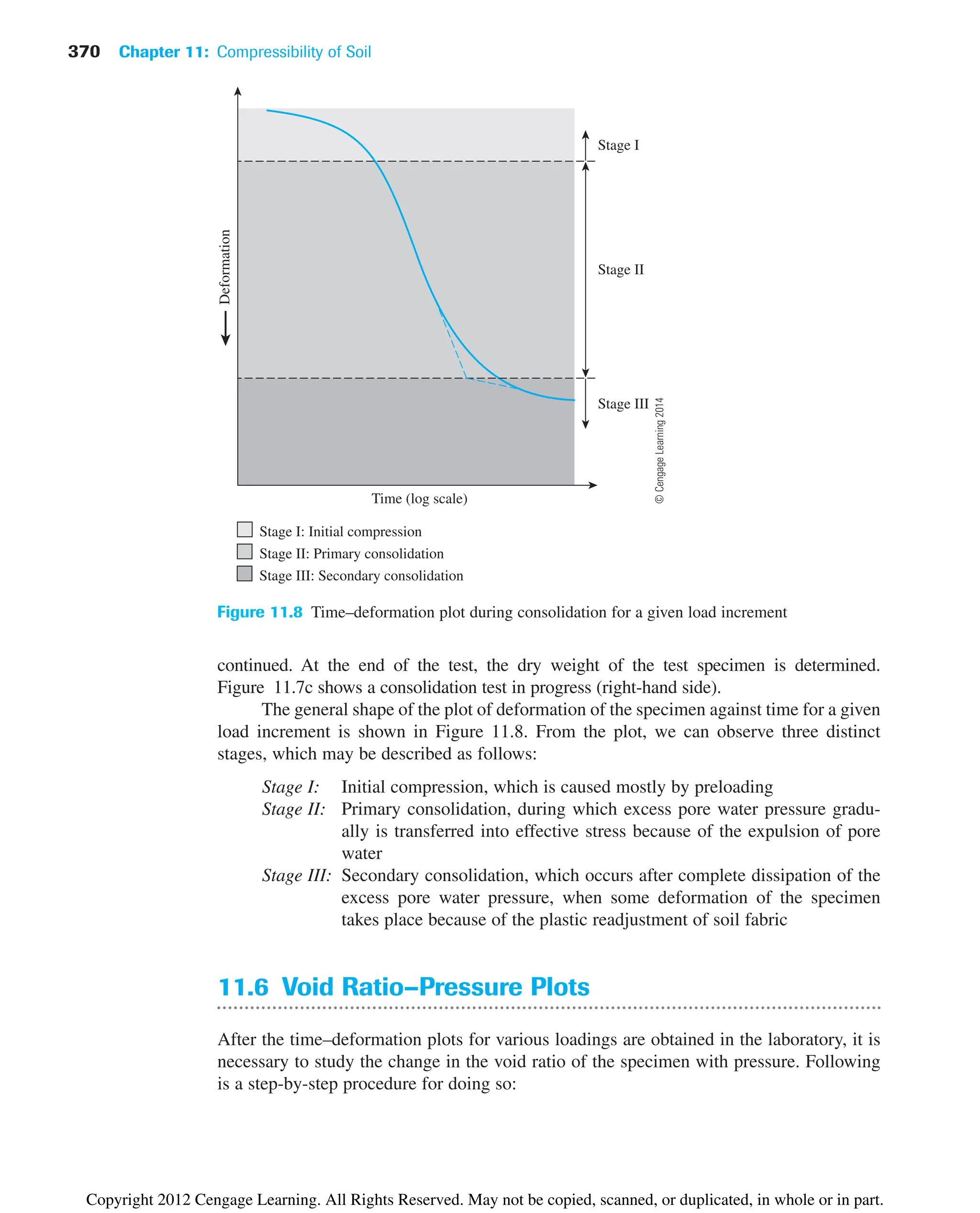
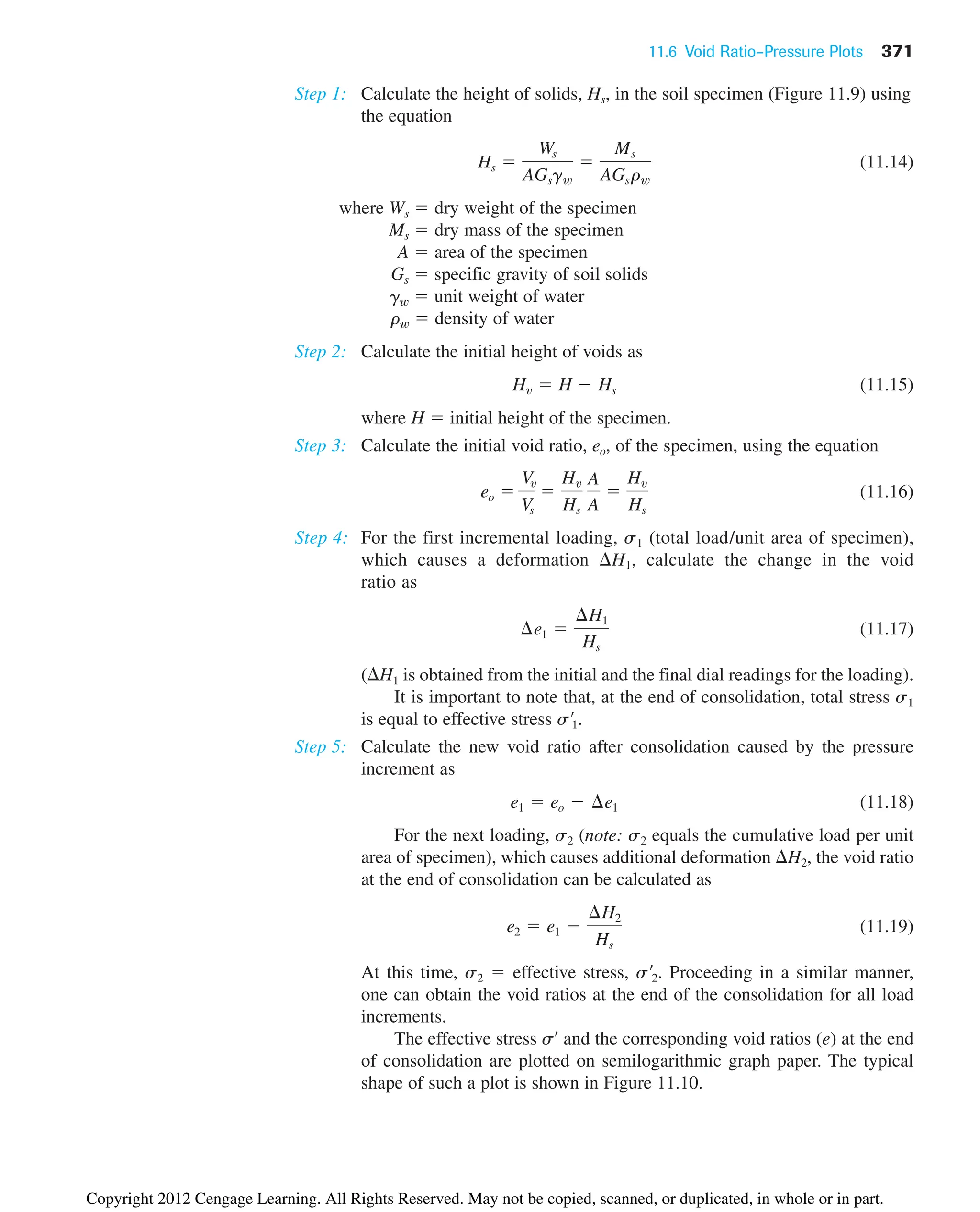
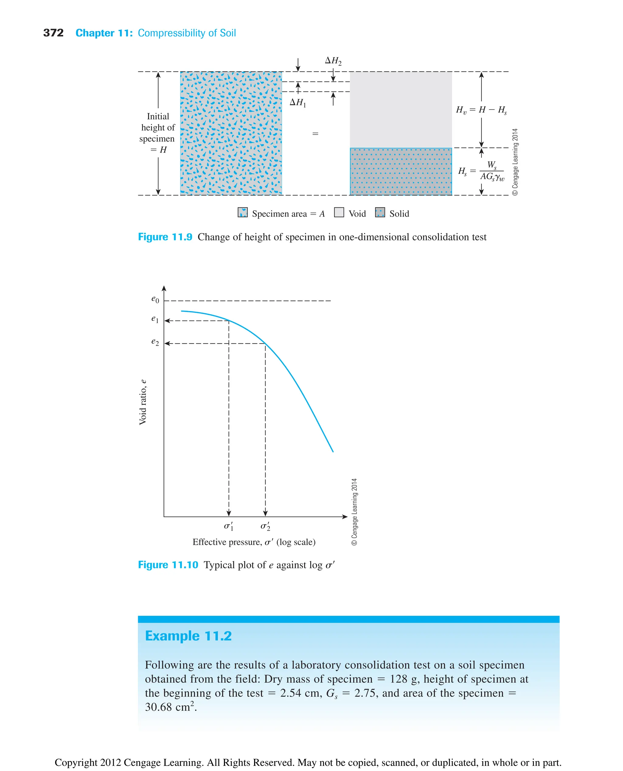
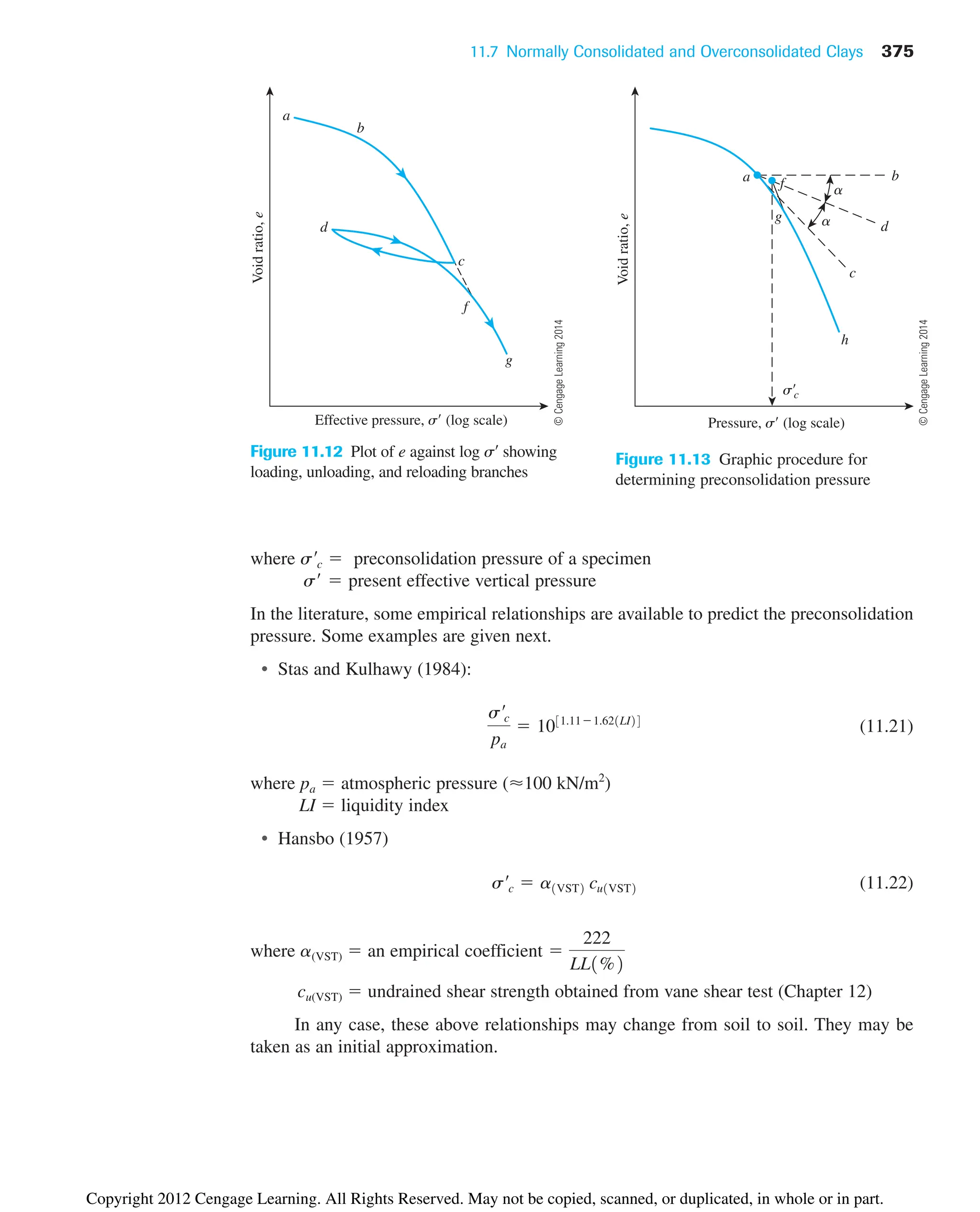
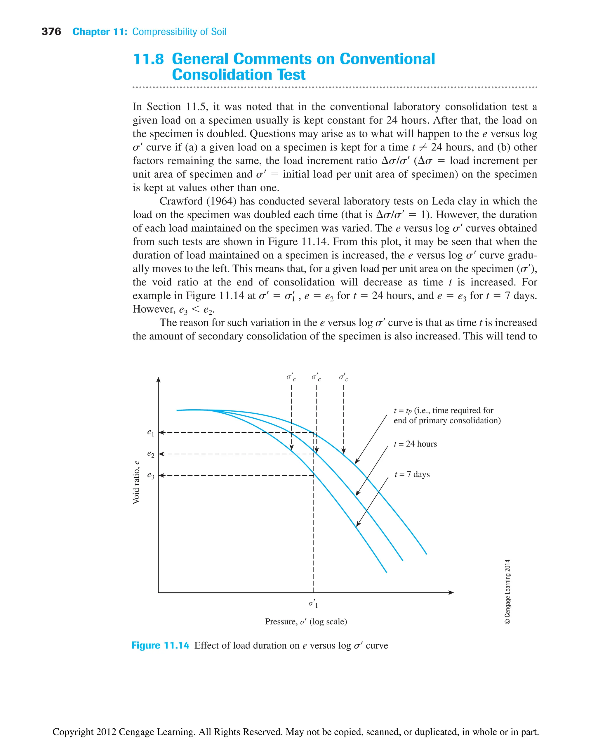
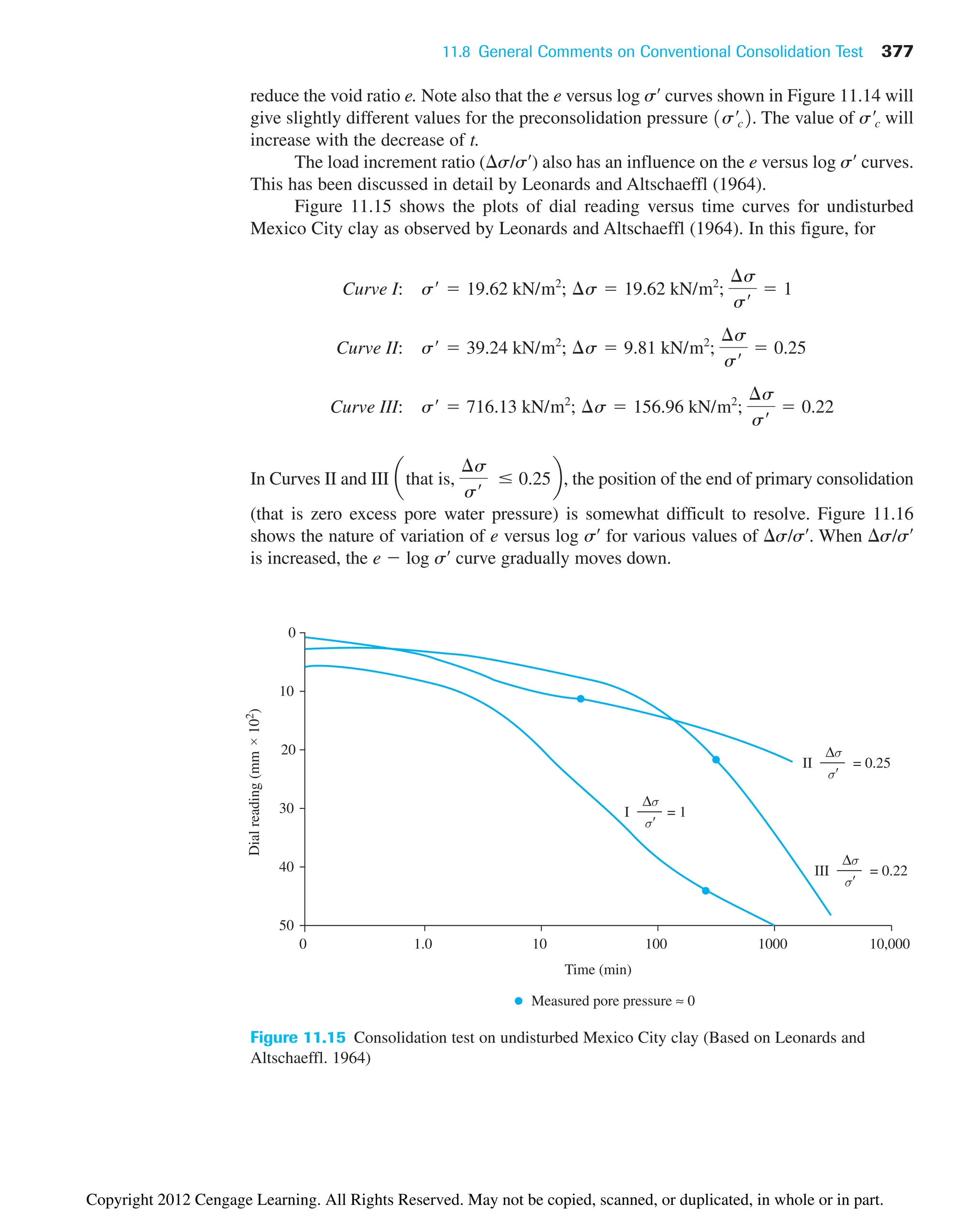
![378 Chapter 11: Compressibility of Soil
σ
Δσ
1
σ
Δσ
σ
Δσ
= 1
1
Pressure, σ (log scale)
Void
ratio,
e
Figure 11.16 Effect of load increment ratio on e versus log s¿ curve
11.9 Effect of Disturbance on Void Ratio–Pressure
Relationship
A soil specimen will be remolded when it is subjected to some degree of disturbance. This
remolding will result in some deviation of the e-log s¿ plot as observed in the laboratory
from the actual behavior in the field. The field e-log s¿ plot can be reconstructed from the
laboratory test results in the manner described in this section (Terzaghi and Peck, 1967).
Normally Consolidated Clay of Low to Medium Plasticity (Figure 11.17)
1. In Figure 11.17, curve 2 is the laboratory e-log s¿ plot. From this plot, determine the
preconsolidation pressure (that is, the present effective overburden pres-
sure). Knowing where , draw vertical line ab.
2. Calculate the void ratio in the field, [Section 11.6, Eq. (11.16)]. Draw horizontal
line cd.
3. Calculate 0.4 and draw line ef. (Note: f is the point of intersection of the line with
curve 2.)
4. Join points f and g. Note that g is the point of intersection of lines ab and cd. This is
the virgin compression curve.
It is important to point out that if a soil is remolded completely, the general position
of the e-log s¿ plot will be as represented by curve 3.
eo
eo
s¿c s¿o
1s¿c2 s¿o
©
Cengage
Learning
2014
Copyright 2012 Cengage Learning. All Rights Reserved. May not be copied, scanned, or duplicated, in whole or in part.](https://image.slidesharecdn.com/principlesofgeotechnicalengineering-8thedition-231222125509-7e44d9bf/75/Principles-of-Geotechnical-Engineering-8th-Edition-pdf-398-2048.jpg)
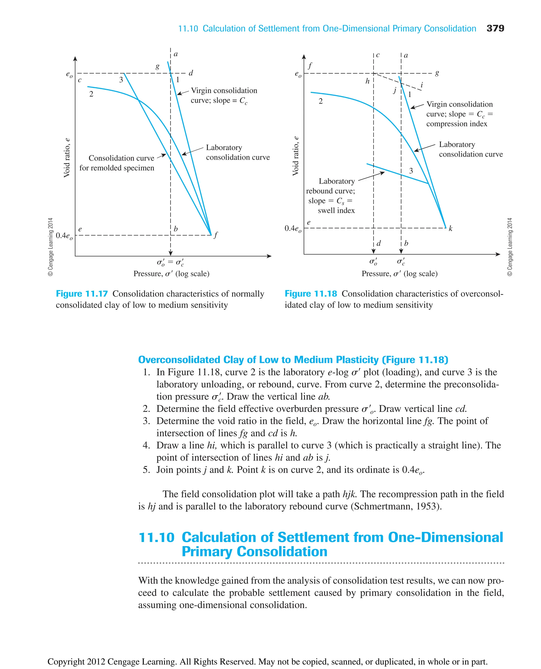
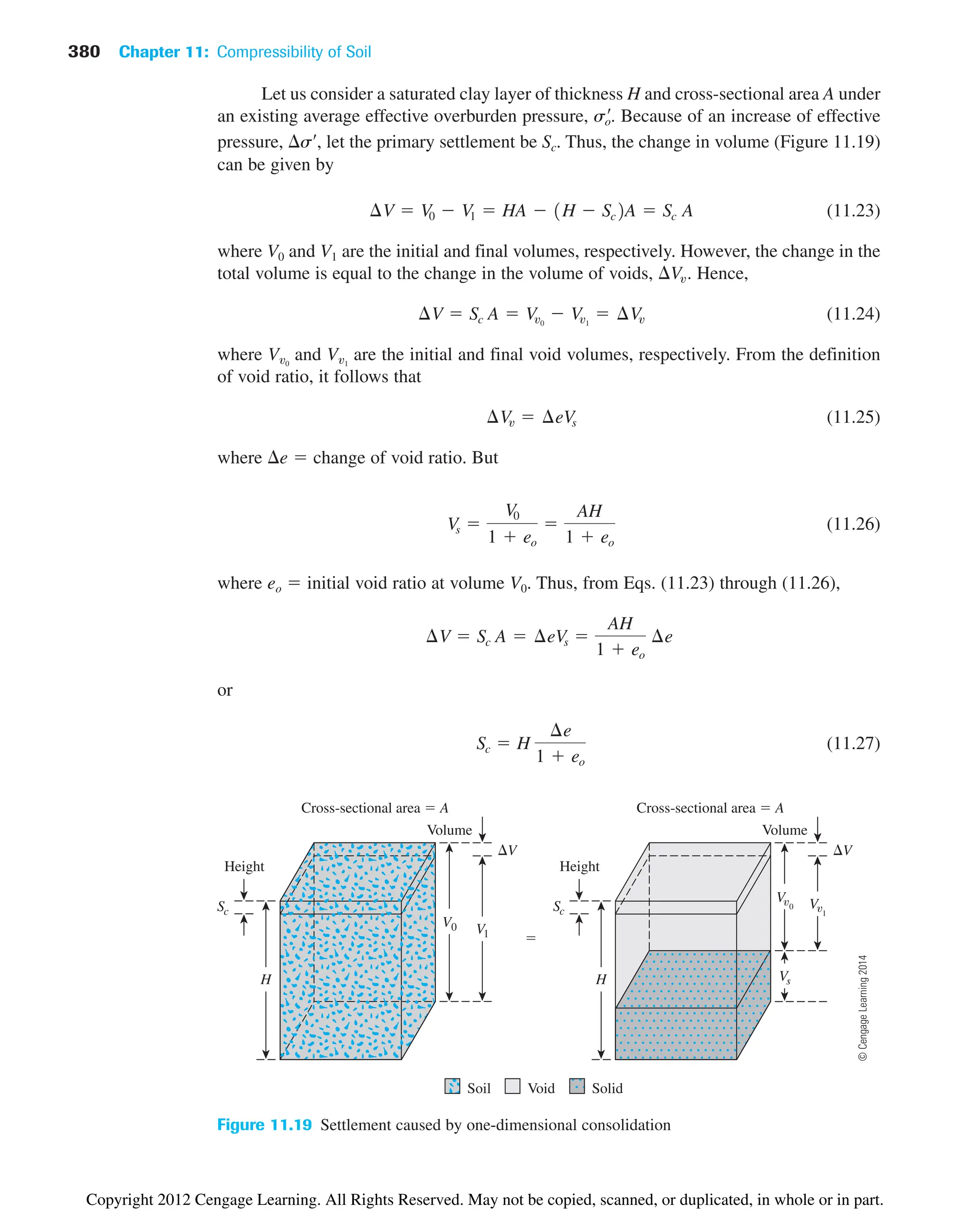
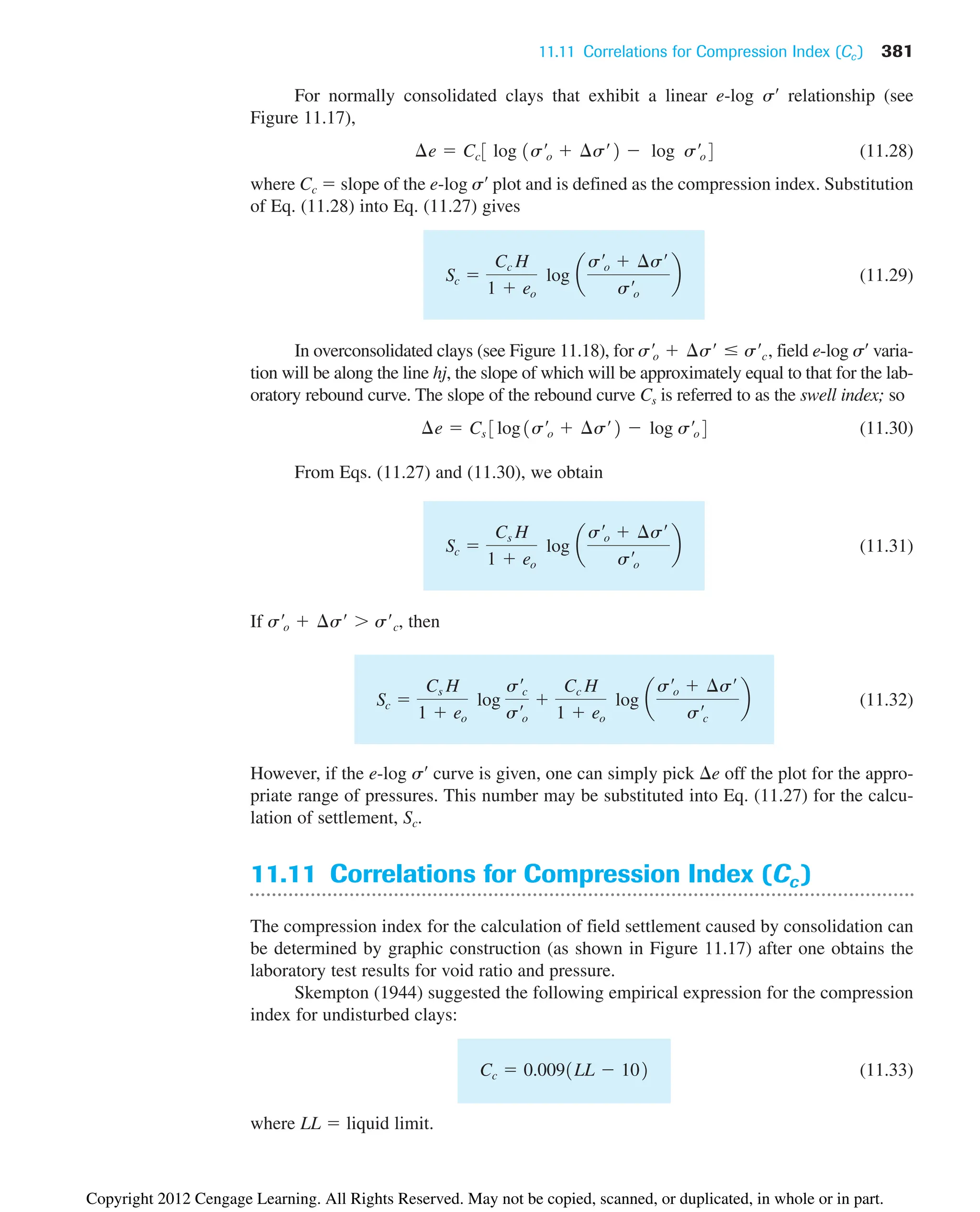
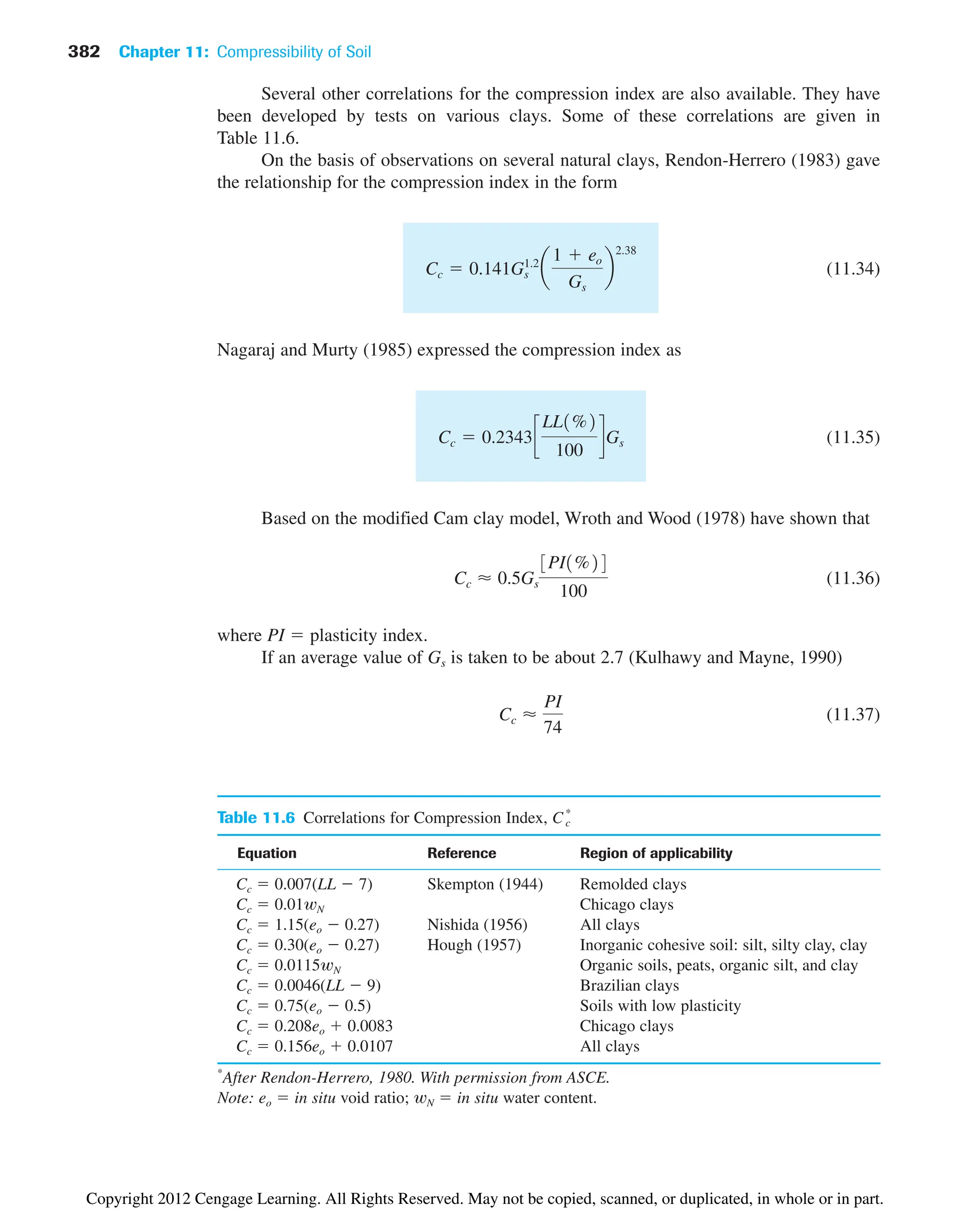
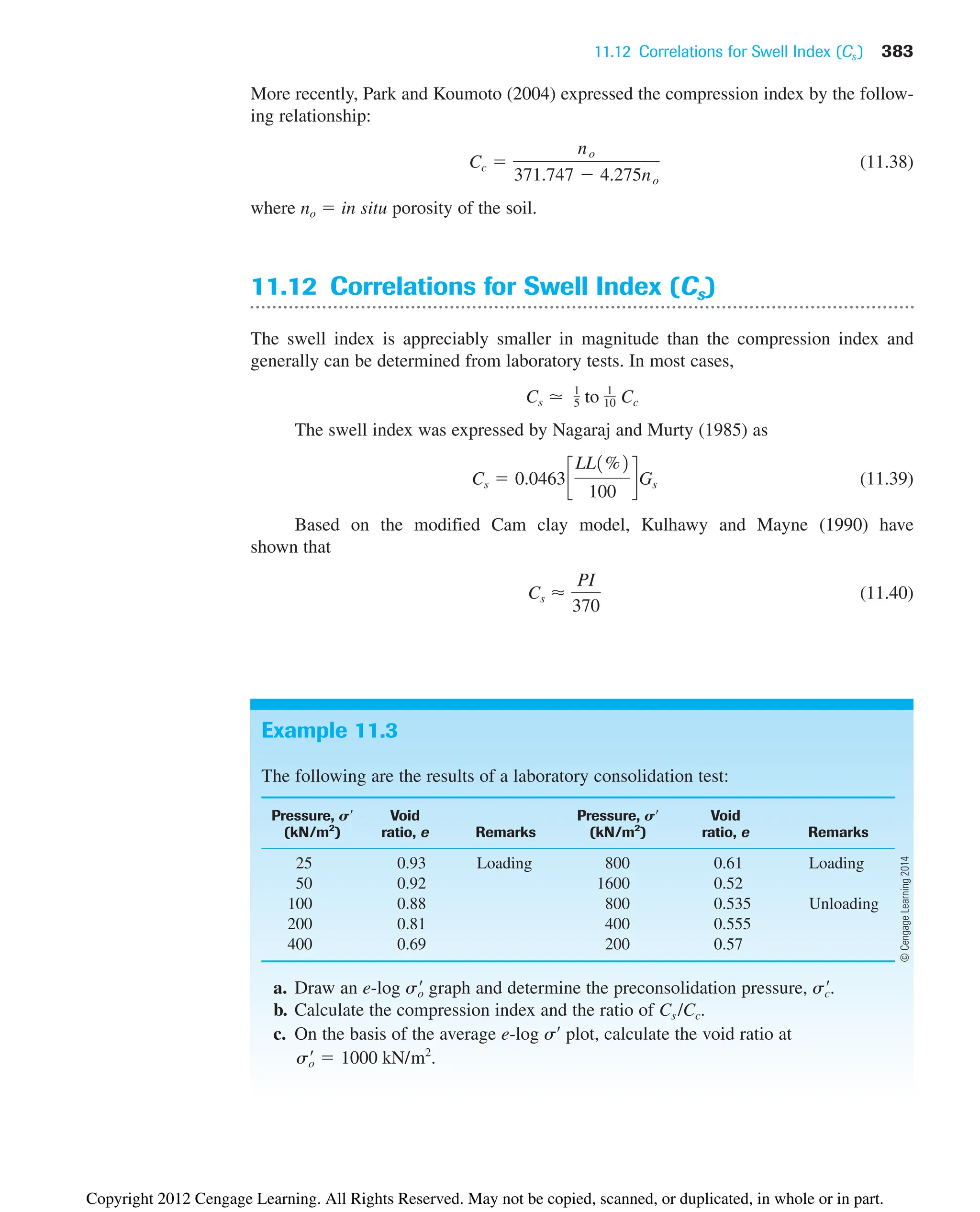

![11.12 Correlations for Swell Index (Cs ) 385
Example 11.4
A soil profile is shown in Figure 11.21. If a uniformly distributed load, s, is applied
at the ground surface, what is the settlement of the clay layer caused by primary con-
solidation if
a. The clay is normally consolidated
b. The preconsolidation pressure
c.
Use Cs ⬇
1
5
Cc.
s¿
c 150 kN/m2
1s¿
c2 200 kN/m2
From the loading branch,
From the unloading branch,
Part c
We know that e1 0.8 at and that Cc 0.33 [part (b)]. Let
. So,
e3 0.8 0.33 log a
1000
200
b ⬇ 0.57
0.33
0.8 e3
log a
1000
200
b
s¿3 1000 kN/m2
s¿1 200 kN/m2
Cc
e1 e3
log
s¿3
s¿1
Cs
Cc
0.04
0.33
0.12
Cs
e1 e2
log
s¿2
s¿1
0.544 0.532
log a
400
200
b
0.0399 ⬇ 0.04
Cc
e1 e2
log
s¿2
s¿1
0.8 0.7
log a
400
200
b
0.33
Copyright 2012 Cengage Learning. All Rights Reserved. May not be copied, scanned, or duplicated, in whole or in part.](https://image.slidesharecdn.com/principlesofgeotechnicalengineering-8thedition-231222125509-7e44d9bf/75/Principles-of-Geotechnical-Engineering-8th-Edition-pdf-405-2048.jpg)
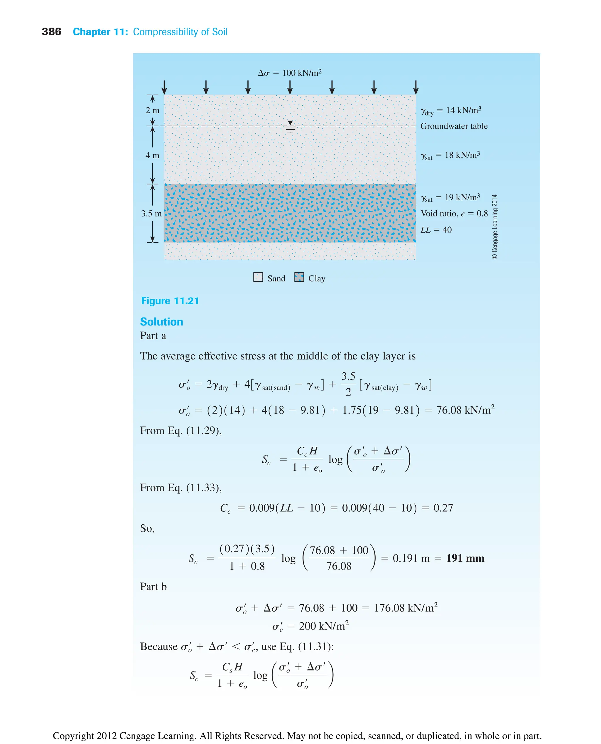
![11.12 Correlations for Swell Index (Cs ) 387
Example 11.5
A soil profile is shown in Figure 11.22a. Laboratory consolidation tests were con-
ducted on a specimen collected from the middle of the clay layer. The field consolida-
tion curve interpolated from the laboratory test results is shown in Figure 11.22b.
Calculate the settlement in the field caused by primary consolidation for a surcharge
of 60 kN/m2
applied at the ground surface.
Solution
The void ratio corresponding to 92.76 kN/m2
(see Figure 11.22b) is 1.045. Hence,
e 1.1 1.045 0.055. We have
[Eq. (11.27)]
So,
Sc 8
10.0552
1 1.1
0.21 m 210 mm
Settlement 1Sc2 H
¢e
1 eo
sO¿ ¢s¿ 32.76 60 92.76 kN/m2
¢s¿ 60 kN/m2
eo 1.1
32.76 kN/m2
s¿o 1421gsat gw2 4118.0 9.812
Part c
Because use Eq. (11.32):
⬇ 0.0675 m 67.5 mm
10.054213.52
1.8
log a
150
76.08
b
10.27213.52
1.8
log a
176.08
150
b
Sc
CsH
1 eo
log
s¿c
s¿o
Cc H
1 eo
log a
s¿o ¢s¿
s¿c
b
s¿o s¿c s¿o ¢s¿,
s¿c 150 kN/m2
s¿o ¢s¿ 176.08 kN/m2
s¿o 76.08 kN/m2
Sc
10.054213.52
1 0.8
log a
76.08 100
76.08
b 0.038 m 38 mm
Cs
Cc
5
0.27
5
0.054
Copyright 2012 Cengage Learning. All Rights Reserved. May not be copied, scanned, or duplicated, in whole or in part.](https://image.slidesharecdn.com/principlesofgeotechnicalengineering-8thedition-231222125509-7e44d9bf/75/Principles-of-Geotechnical-Engineering-8th-Edition-pdf-407-2048.jpg)
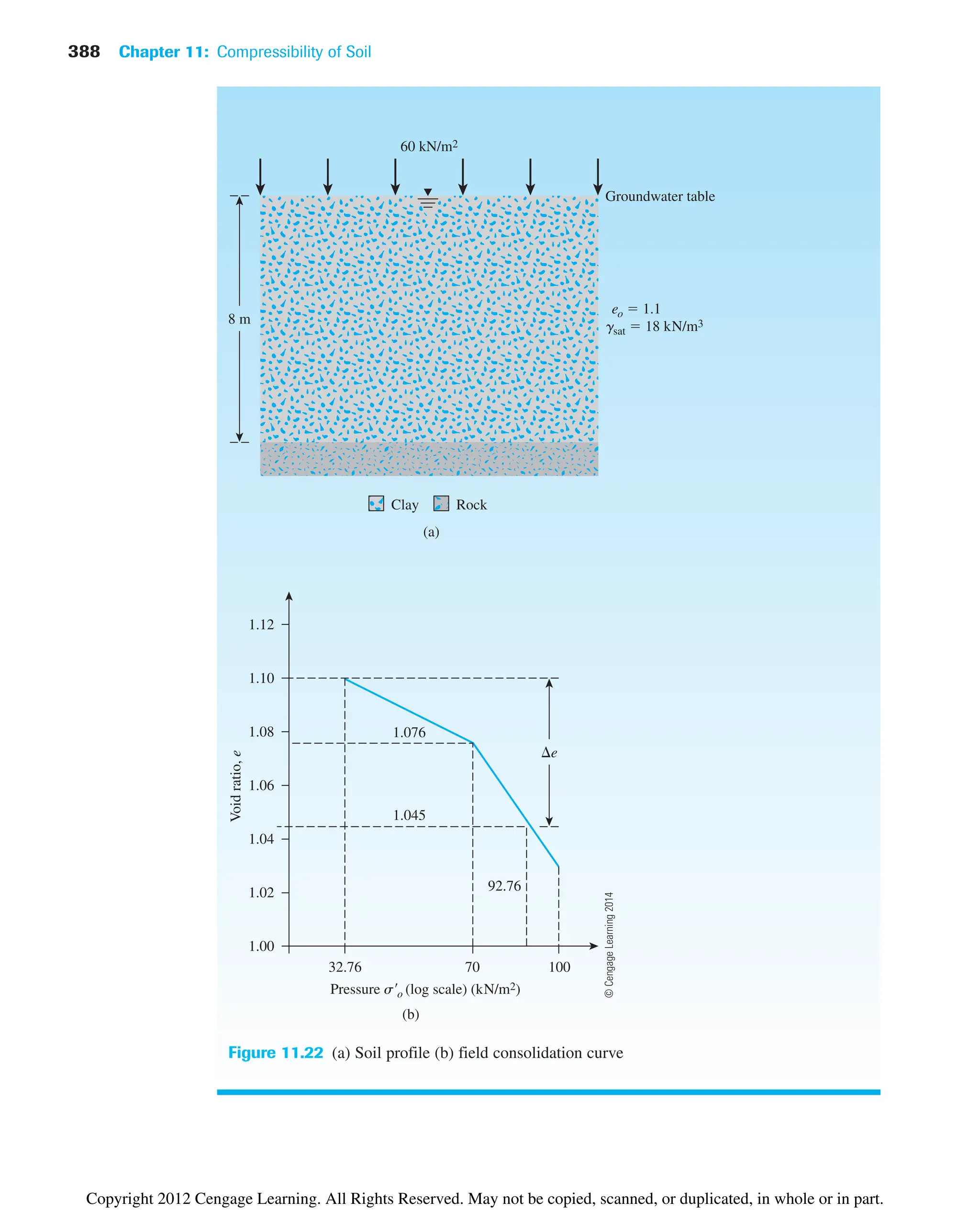
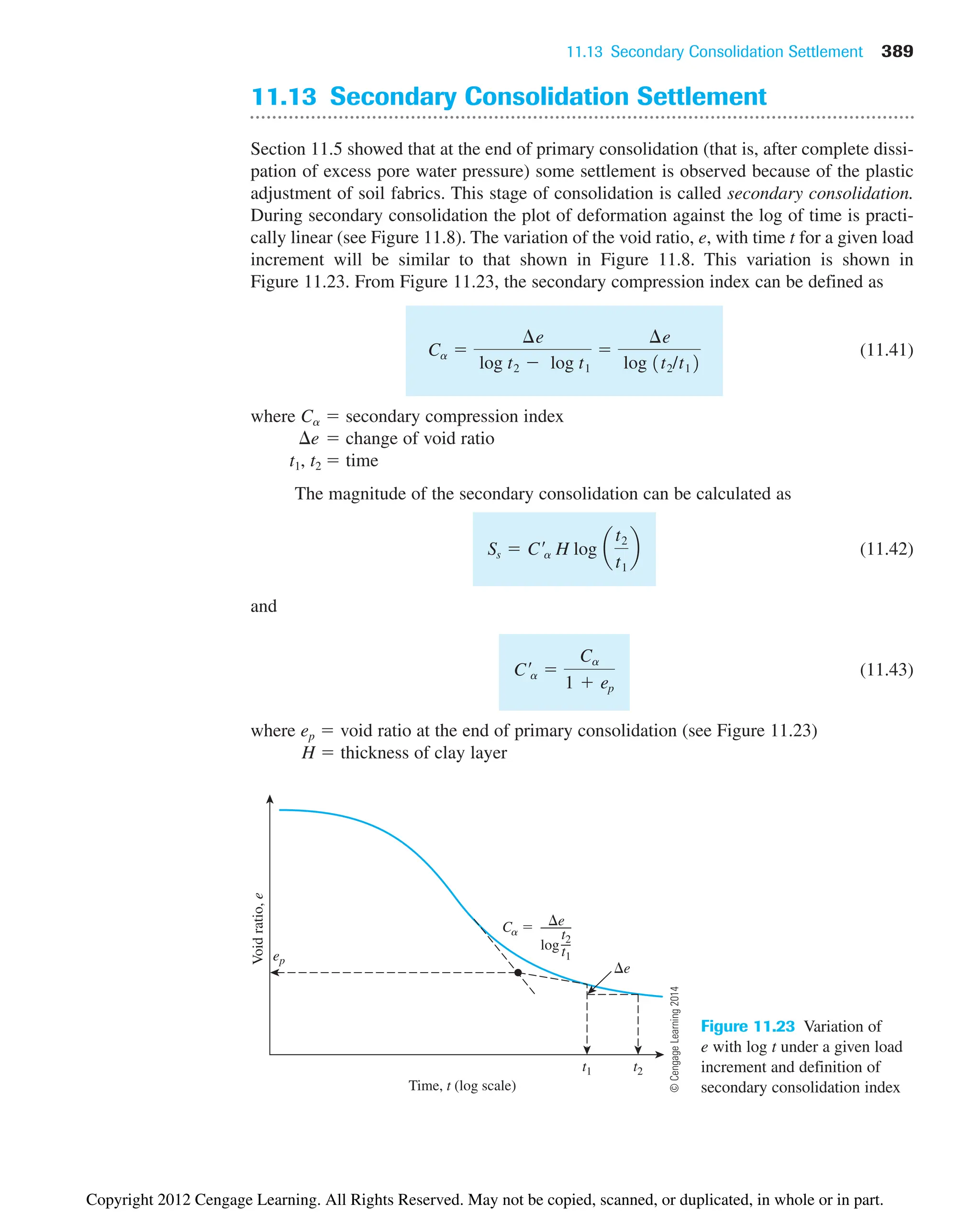
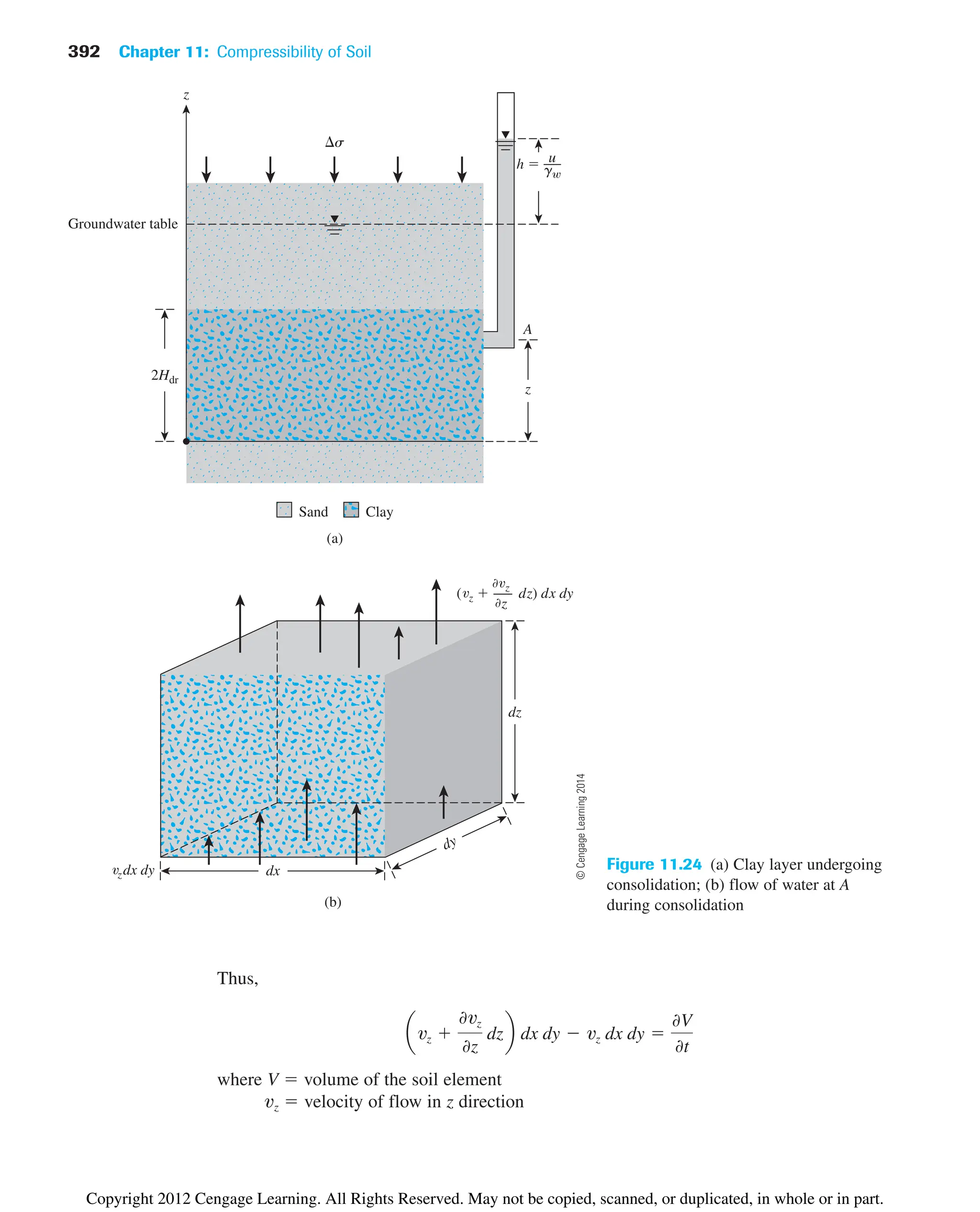
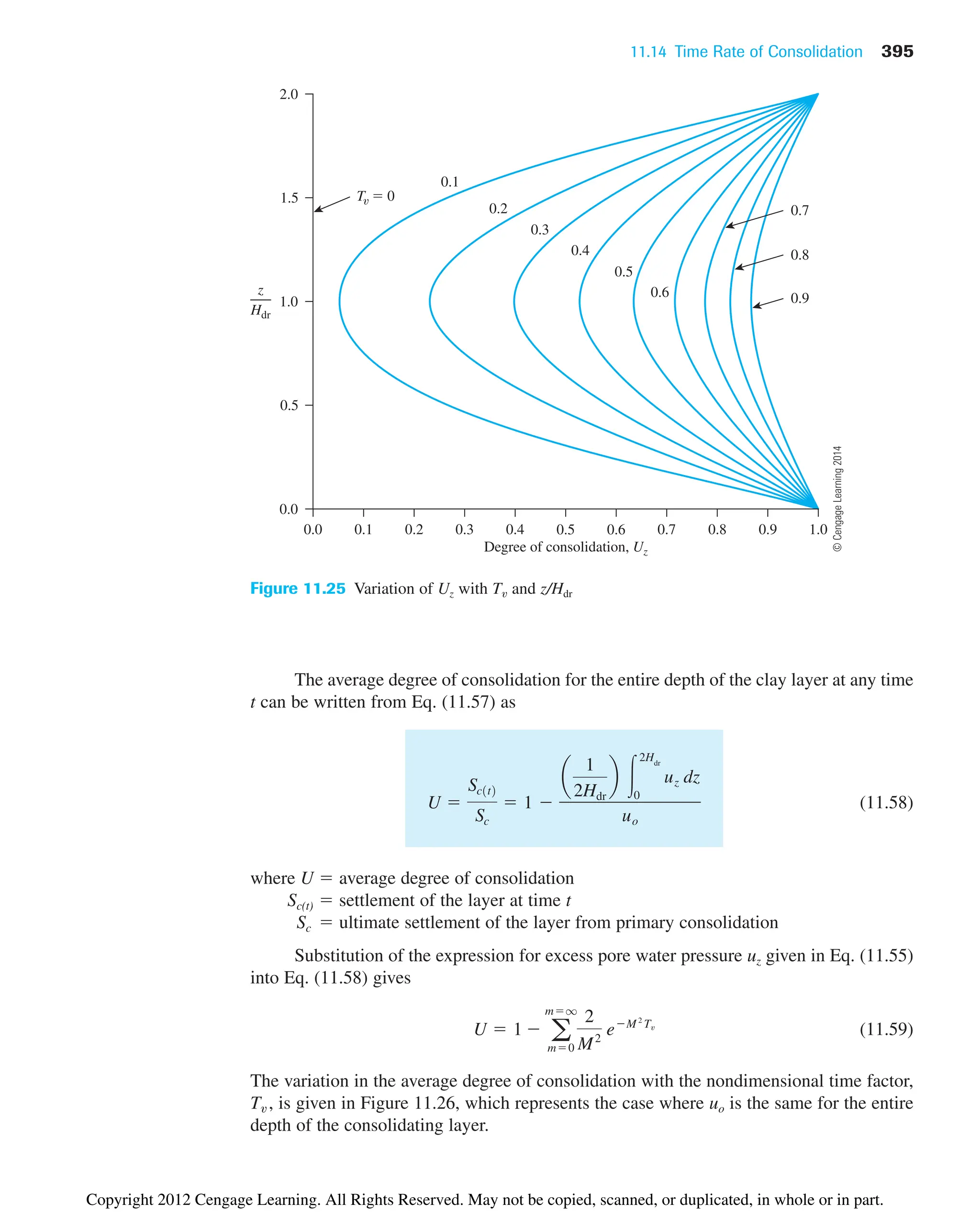
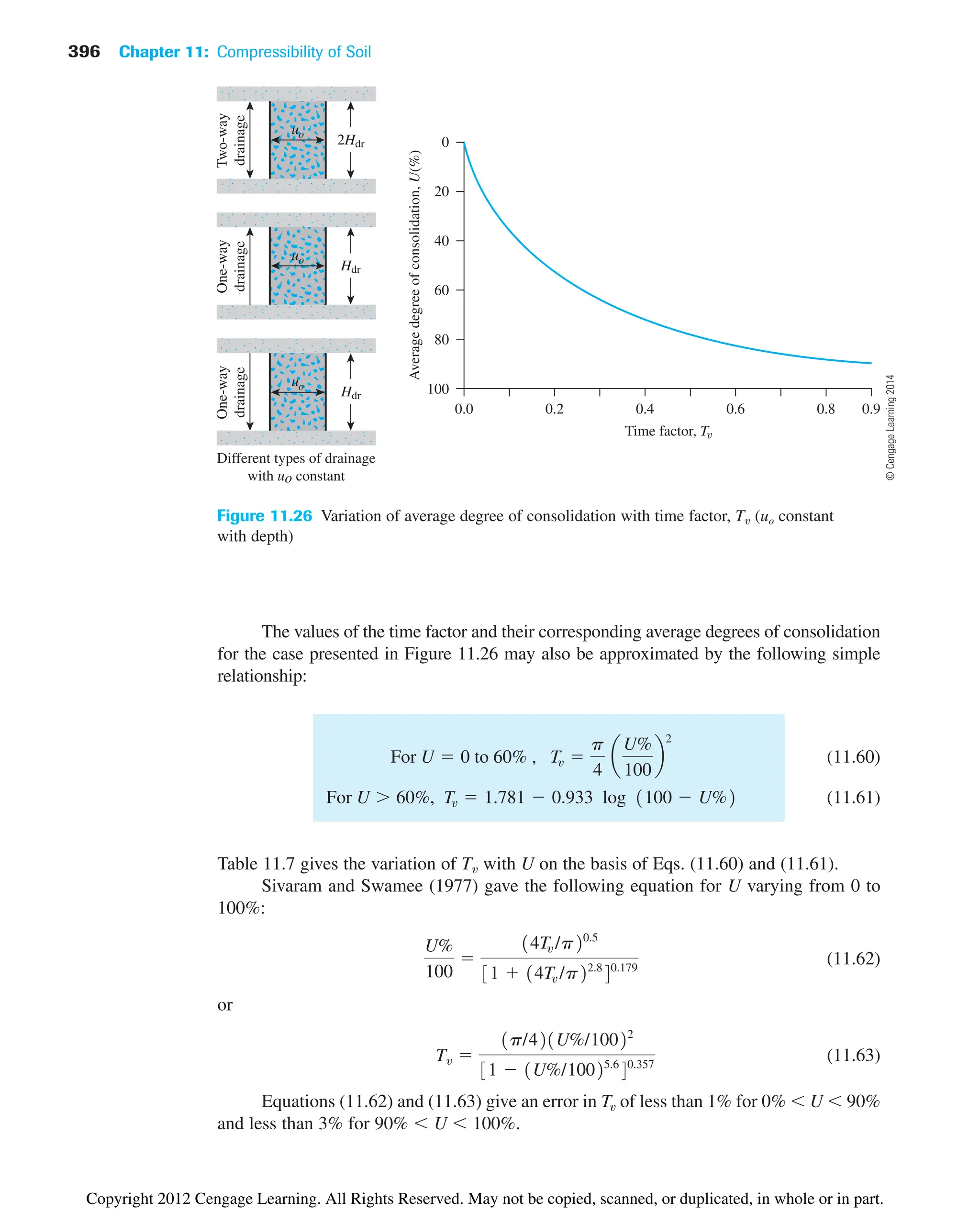
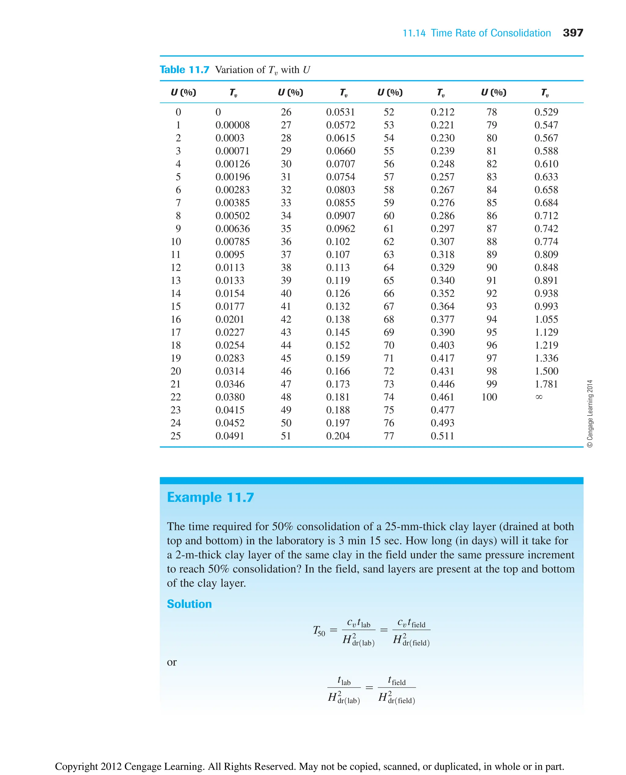
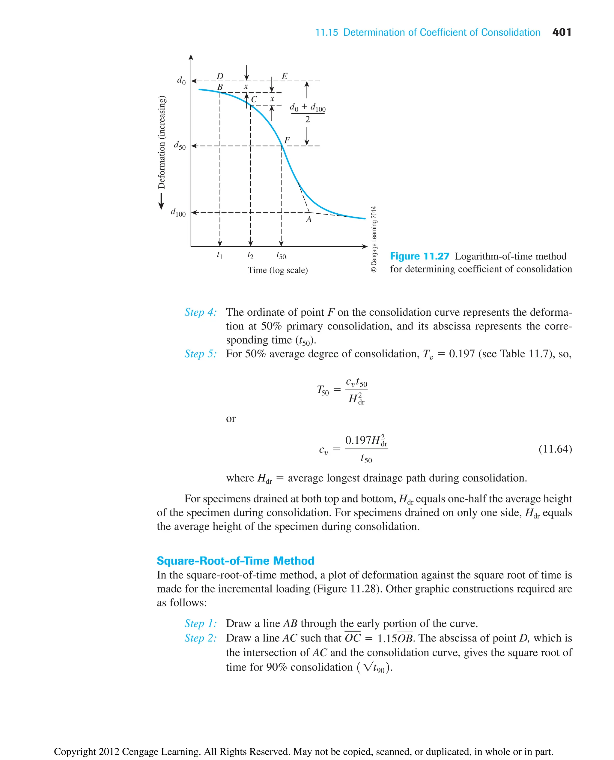
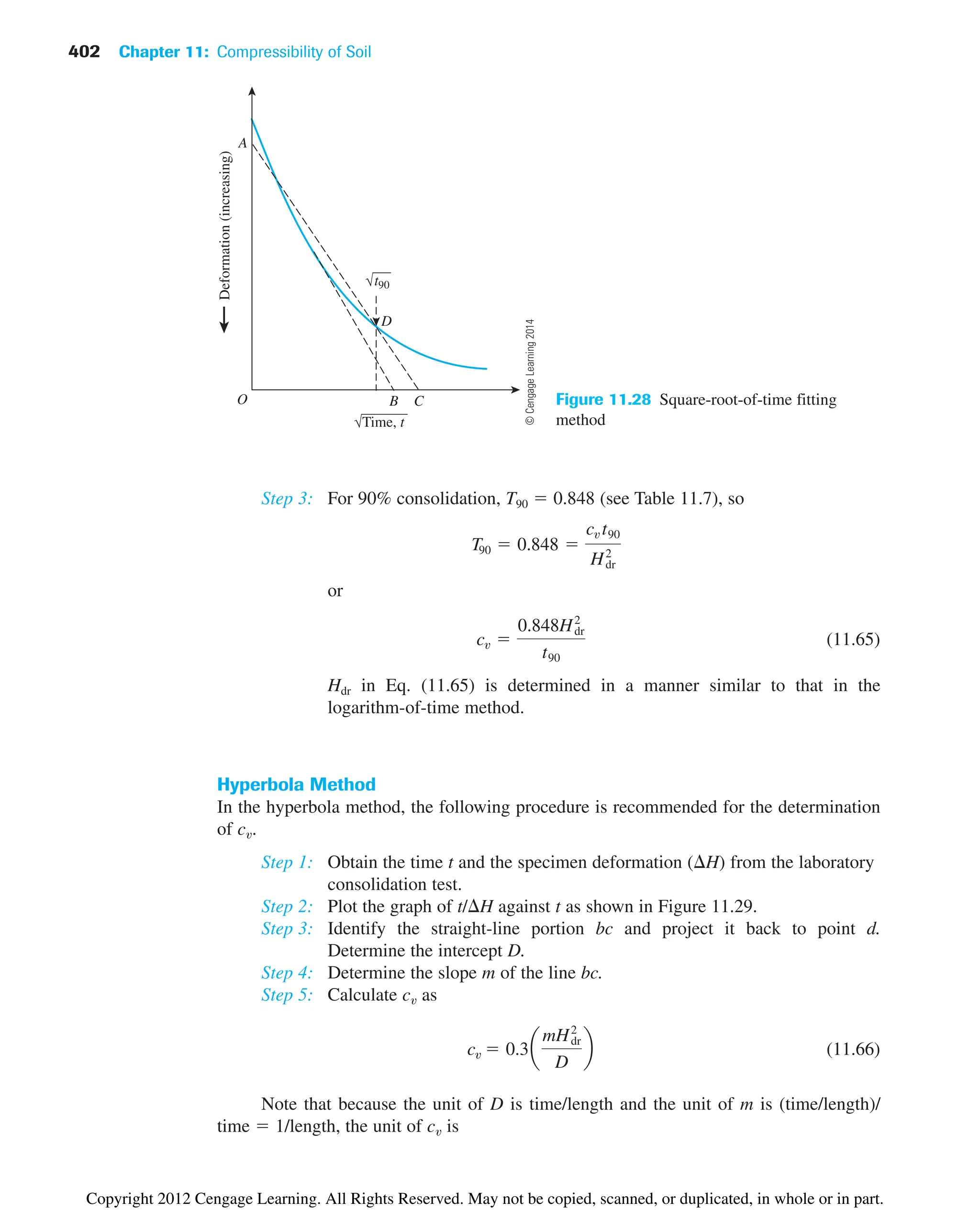
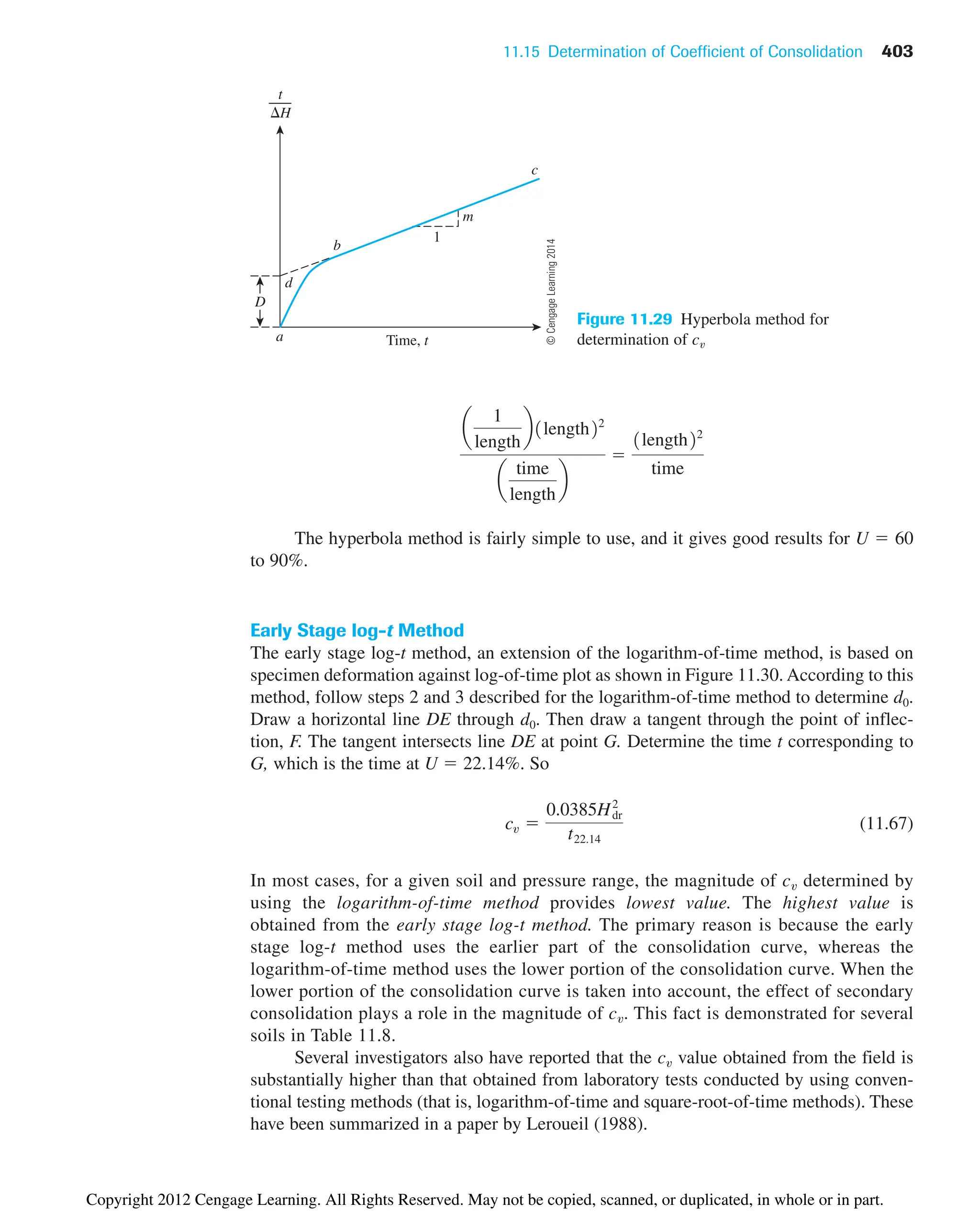
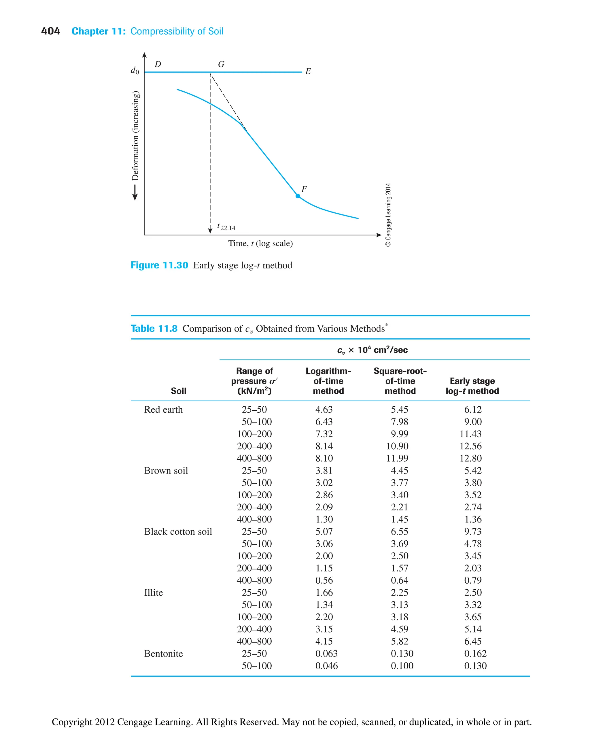
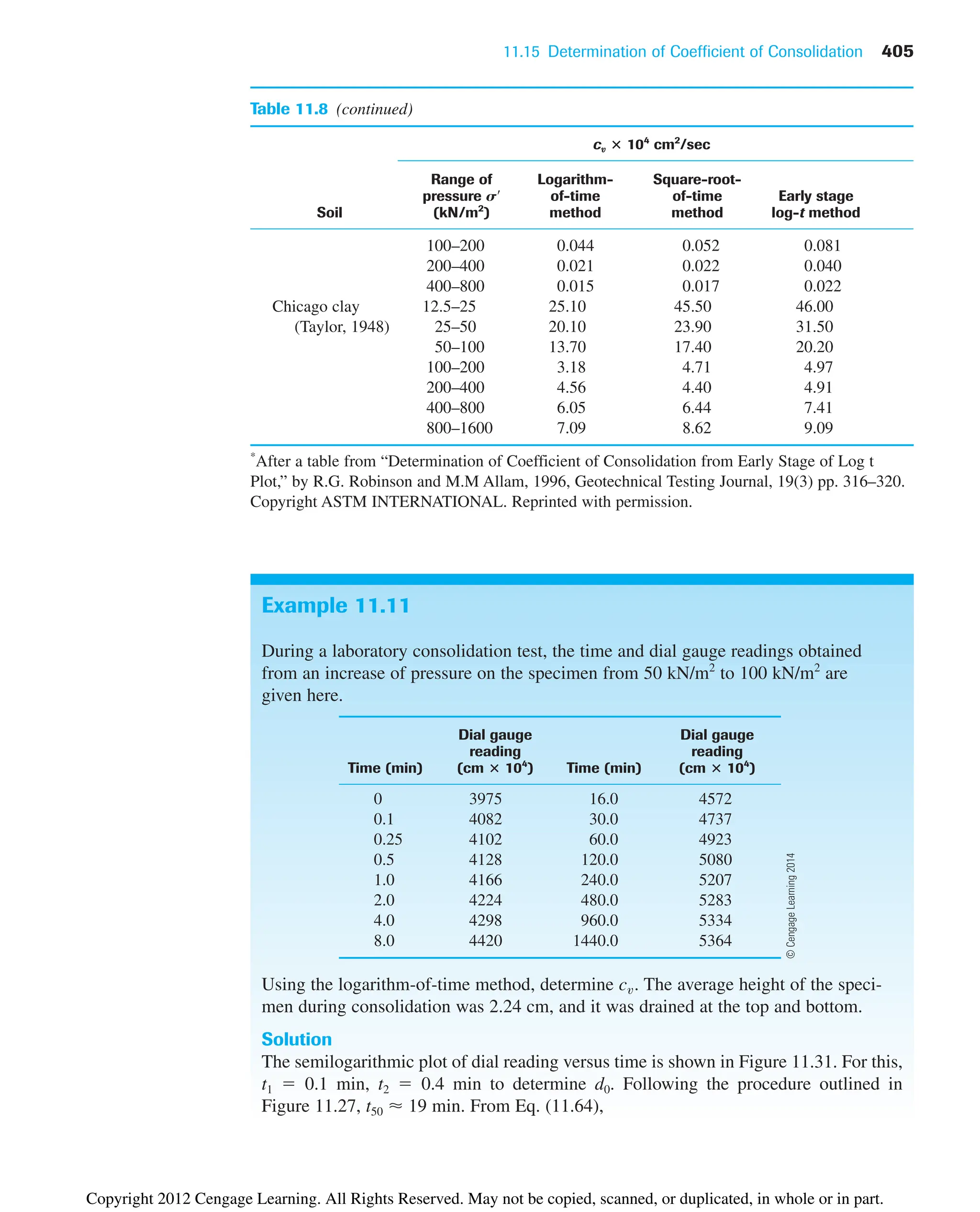
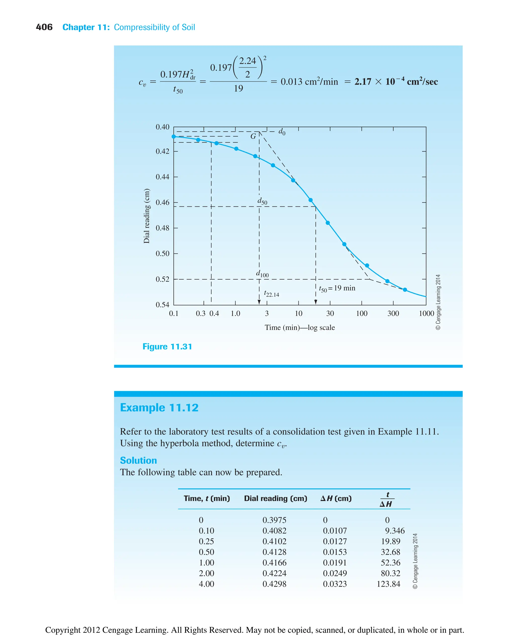
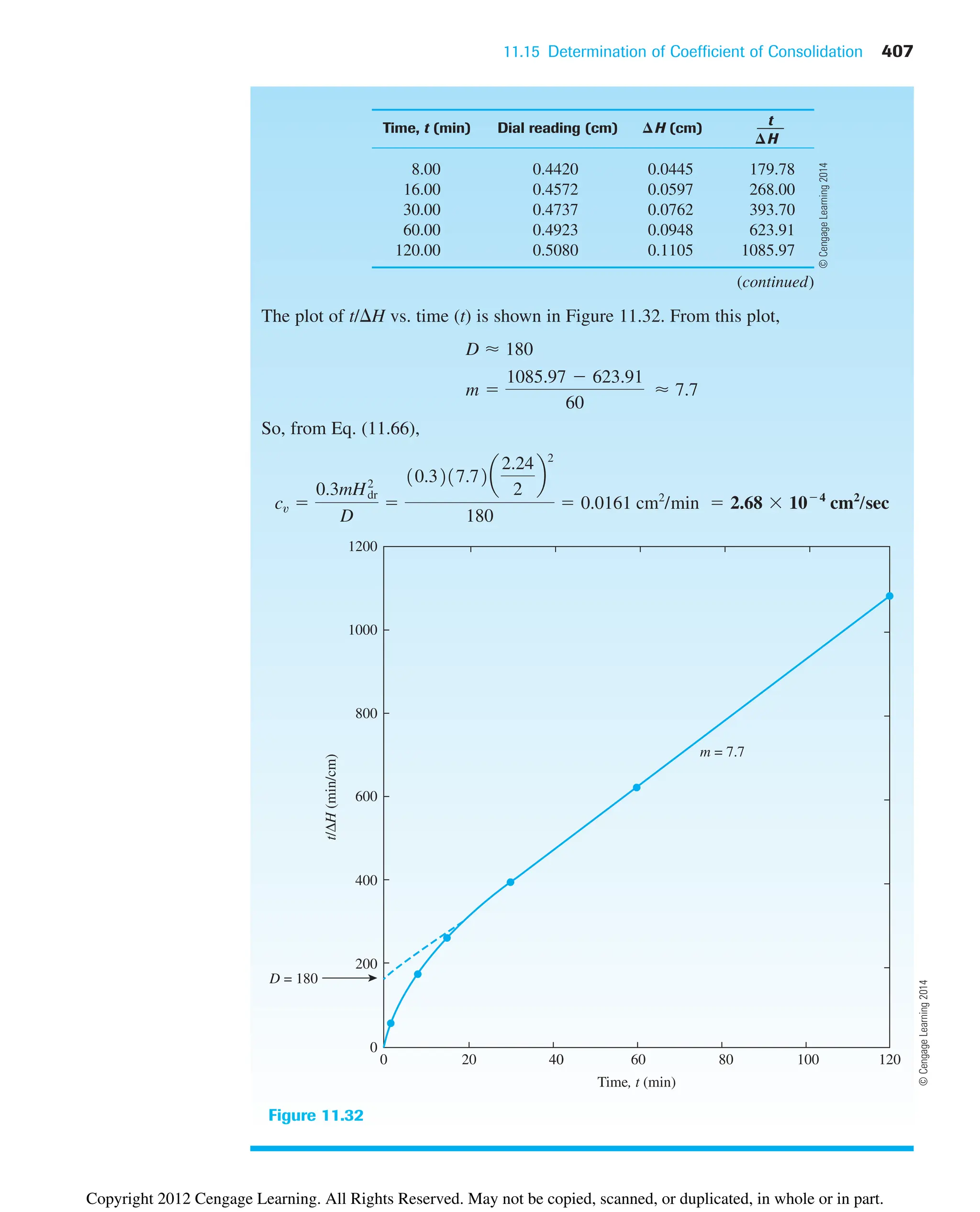
![408 Chapter 11: Compressibility of Soil
Example 11.13
Refer to the laboratory test results of a consolidation test given in Example 11.11.
Using the earth stage log-t method, determine cv.
Solution
Refer to Figure 11.31. A tangent is drawn through the point of inflection. It intersects
the do line at G. The time corresponding to point G is 2.57 min. From Eq. (11.67),
0.01879 cm/min 3.13 : 104
cm2
/sec
cv
0.03851Hdr22
t22.14
10.03852a
2.24
2
b
2
2.57
Example 11.14
Calculate the settlement of the 3-m-thick clay layer (Figure 11.33) that will result
from the load carried by a 1.5-m-square footing. The clay is normally consolidated.
Use the weighted average method [Eq. (11.68)] to calculate the average increase of
effective pressure in the clay layer.
11.16 Calculation of Consolidation Settlement
under a Foundation
Chapter 10 showed that the increase in the vertical stress in soil caused by a load applied
over a limited area decreases with depth z measured from the ground surface downward.
Hence to estimate the one-dimensional settlement of a foundation, we can use Eq. (11.29),
(11.31), or (11.32). However, the increase of effective stress, s¿, in these equations should
be the average increase in the pressure below the center of the foundation. The values can
be determined by using the procedure described in Chapter 10.
Assuming that the pressure increase varies parabolically, using Simpson’s rule, we
can estimate the value of as
(11.68)
where , , and represent the increase in the effective pressure at the top,
middle, and bottom of the layer, respectively.
¢s¿
b
¢s¿
m
¢s¿
t
¢s¿
av
¢s¿
t 4¢s¿
m ¢s¿
b
6
¢s¿
av
Copyright 2012 Cengage Learning. All Rights Reserved. May not be copied, scanned, or duplicated, in whole or in part.](https://image.slidesharecdn.com/principlesofgeotechnicalengineering-8thedition-231222125509-7e44d9bf/75/Principles-of-Geotechnical-Engineering-8th-Edition-pdf-428-2048.jpg)
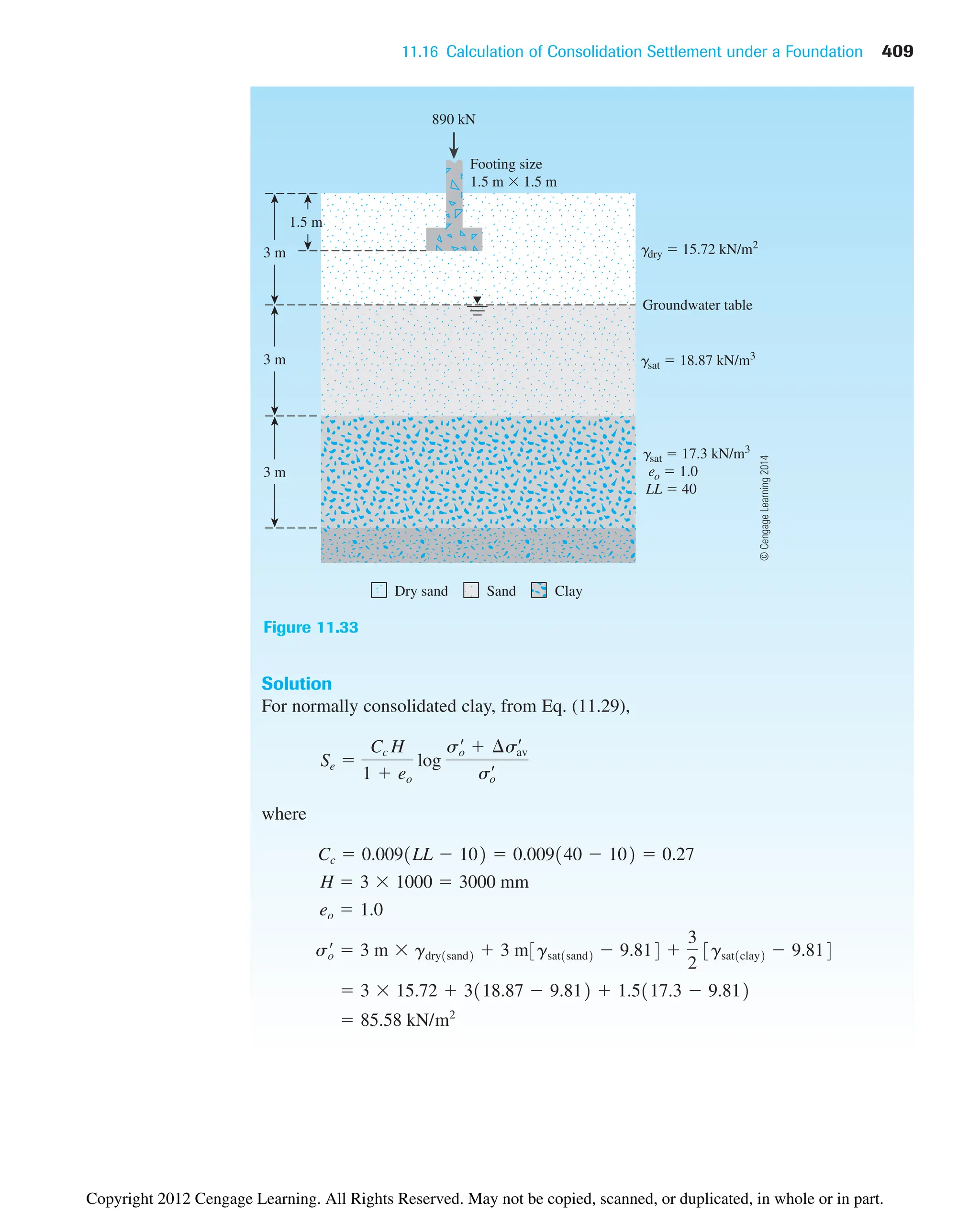
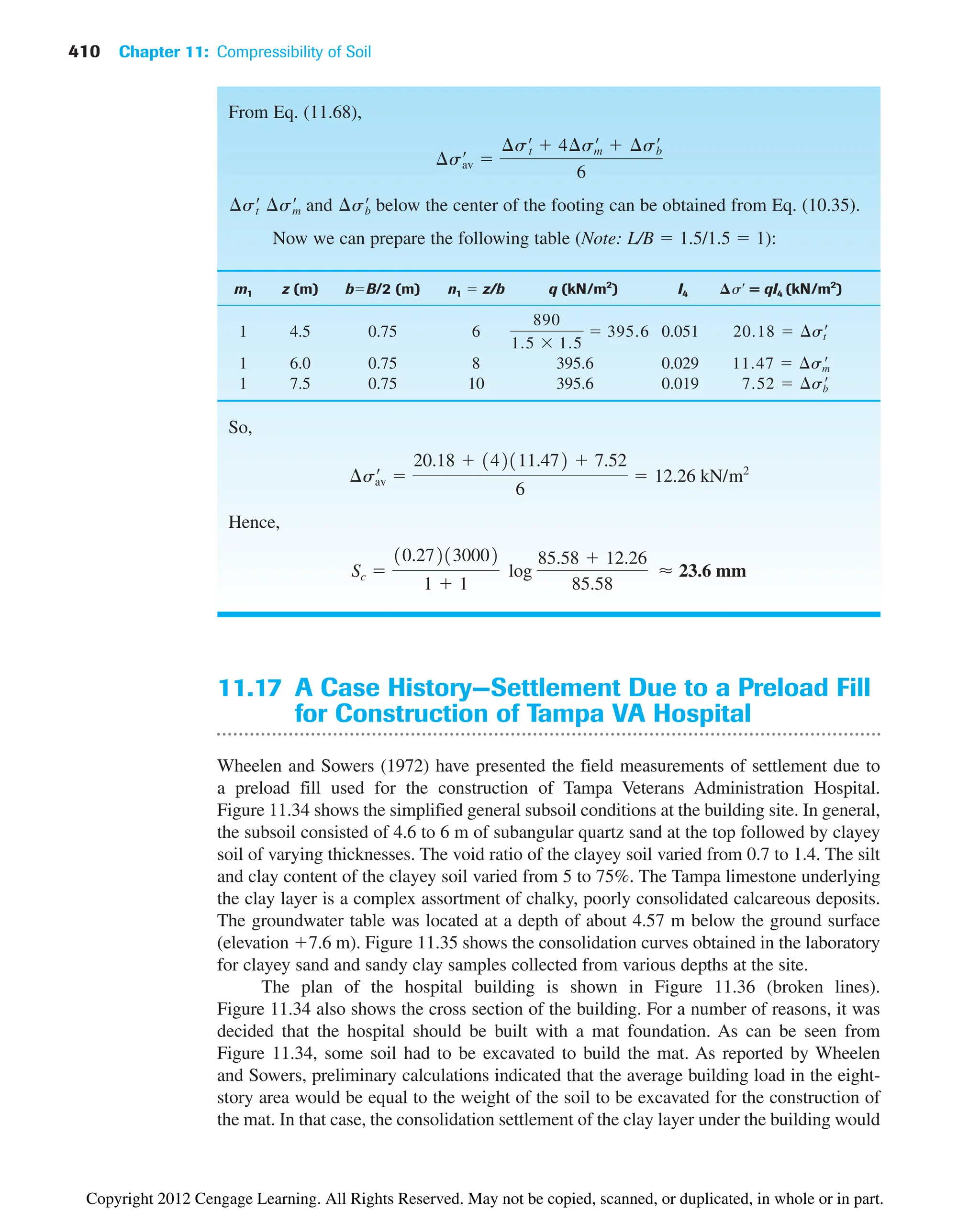
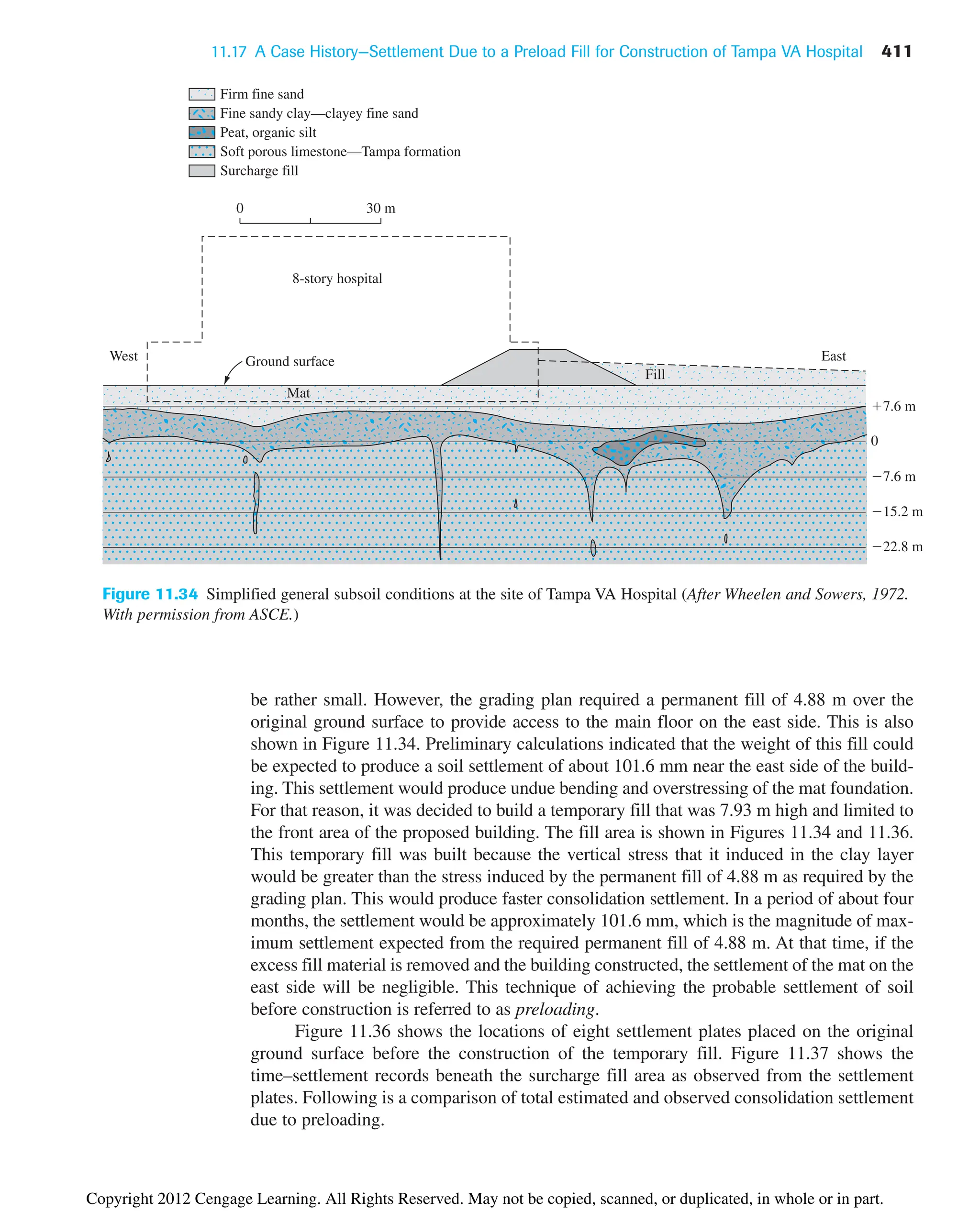
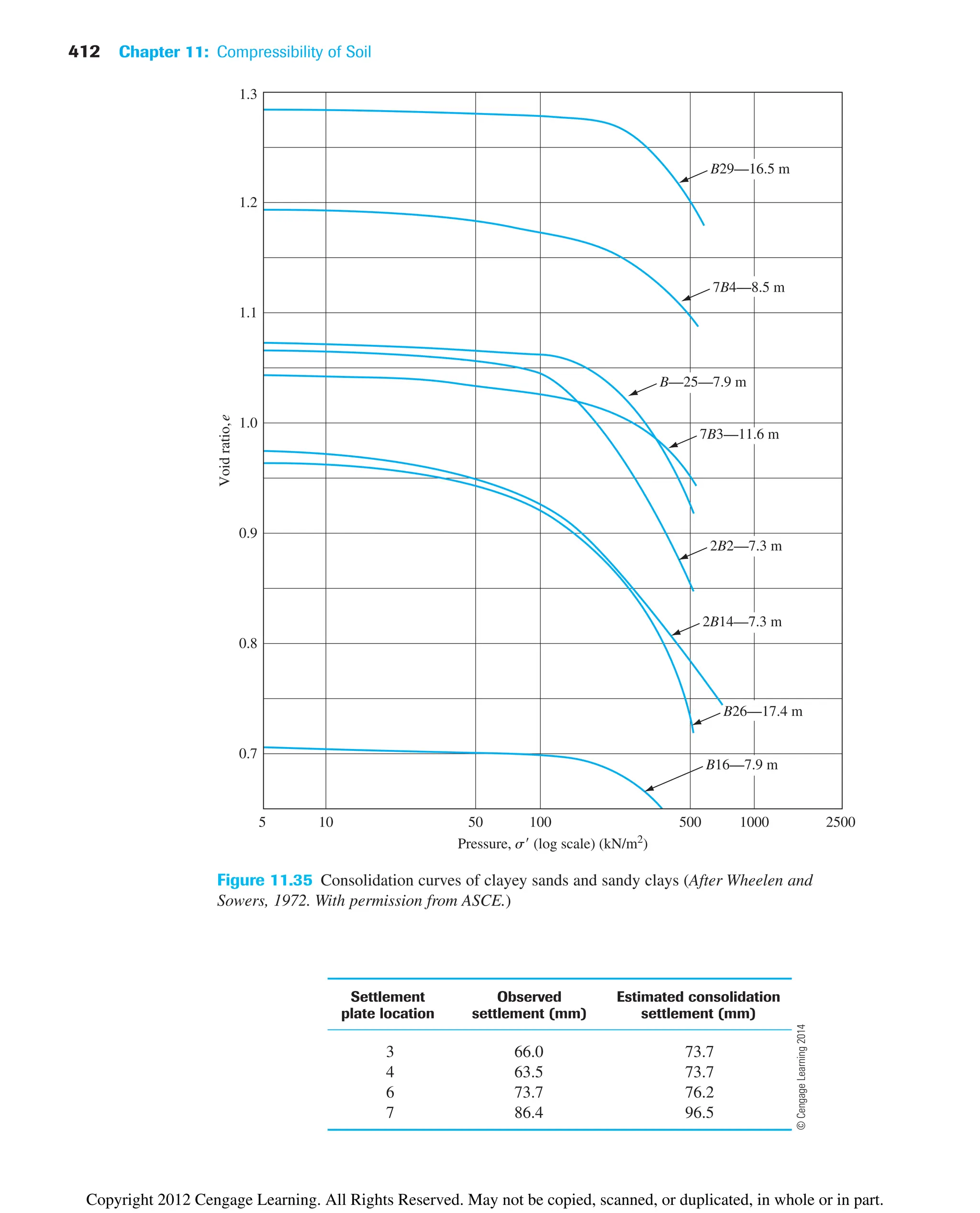
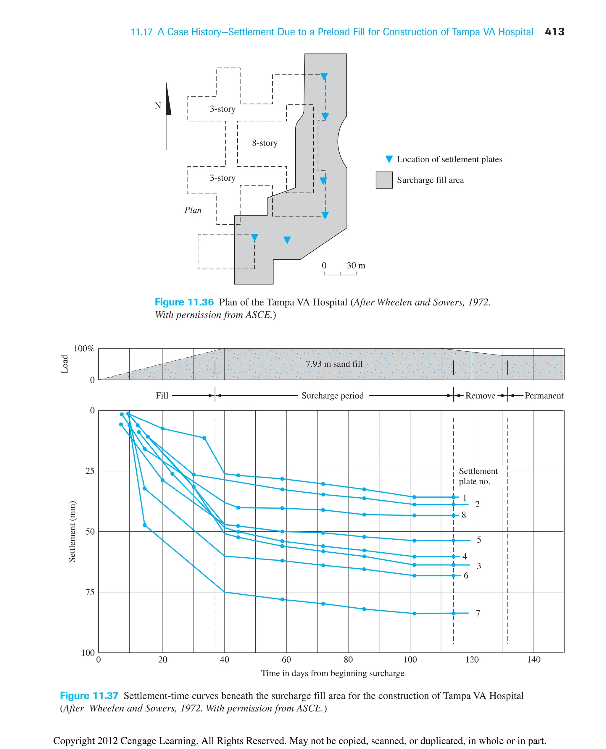
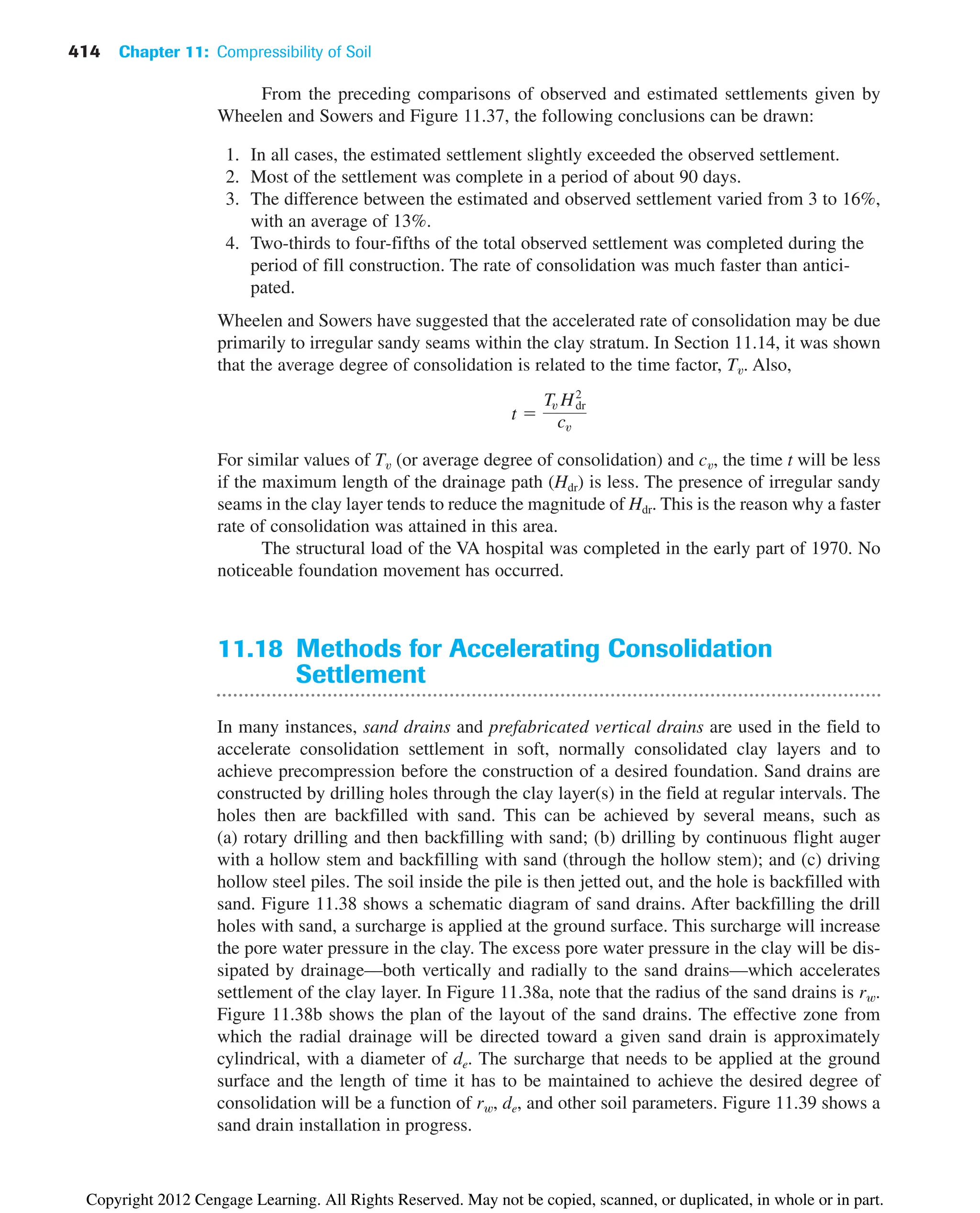
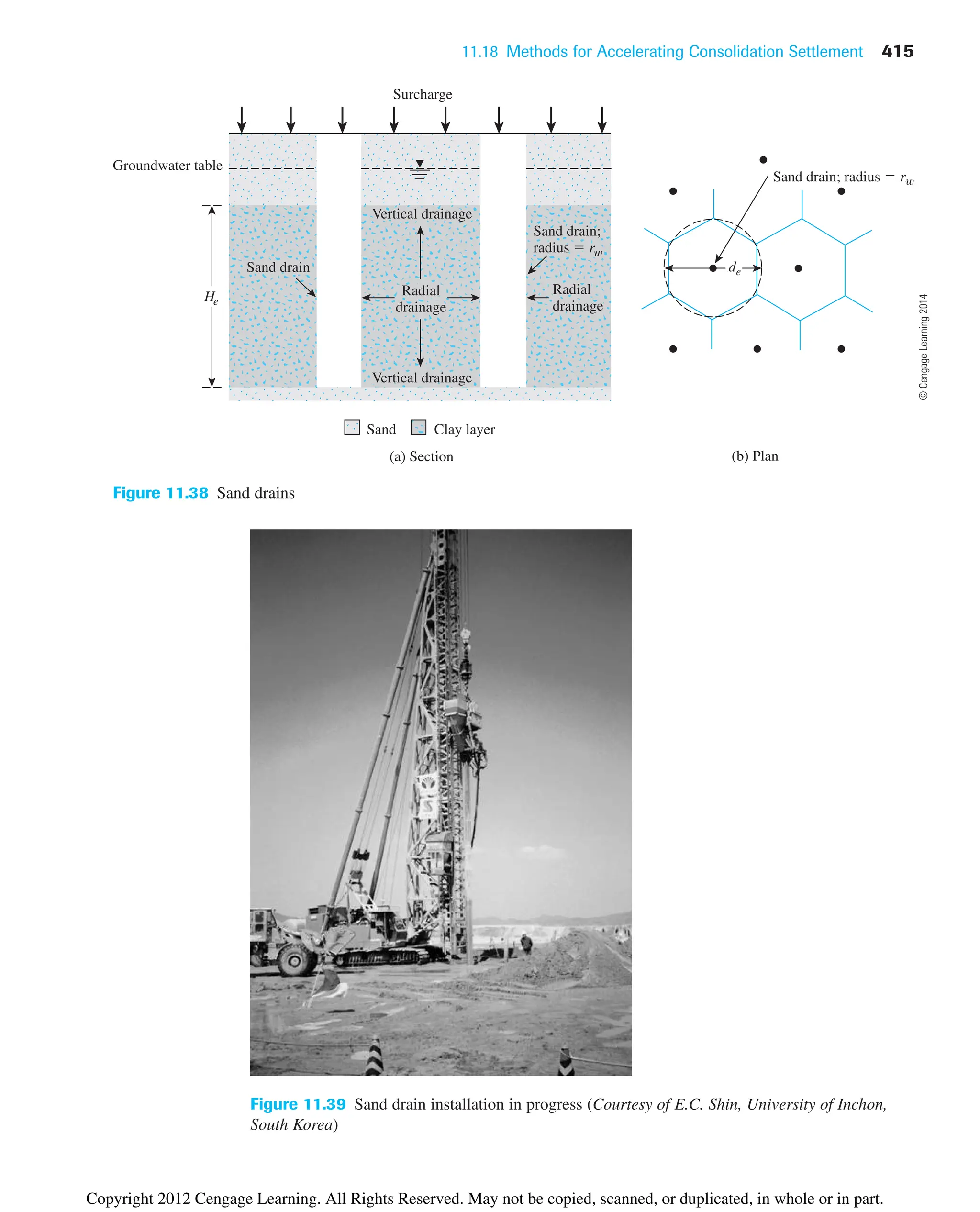
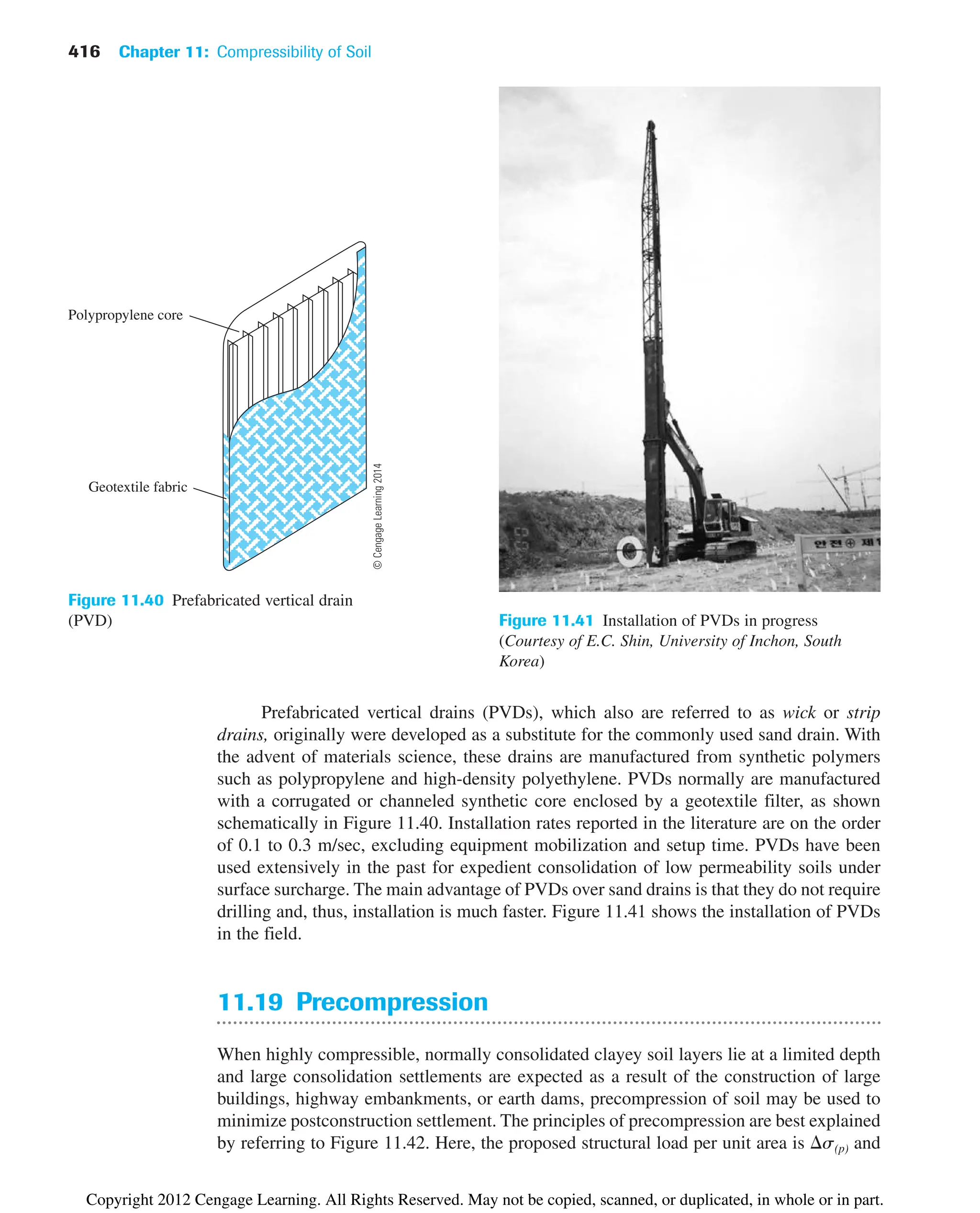
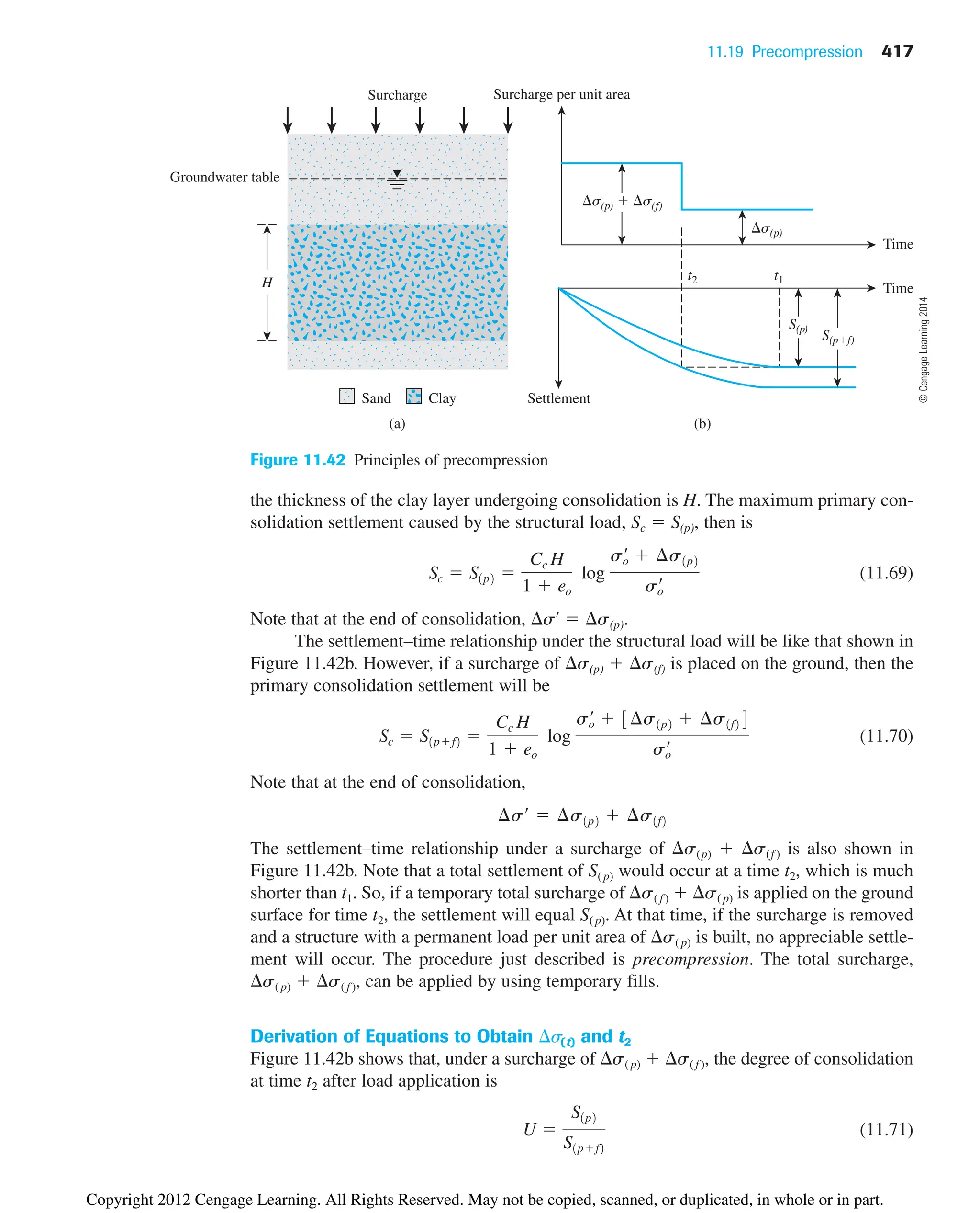
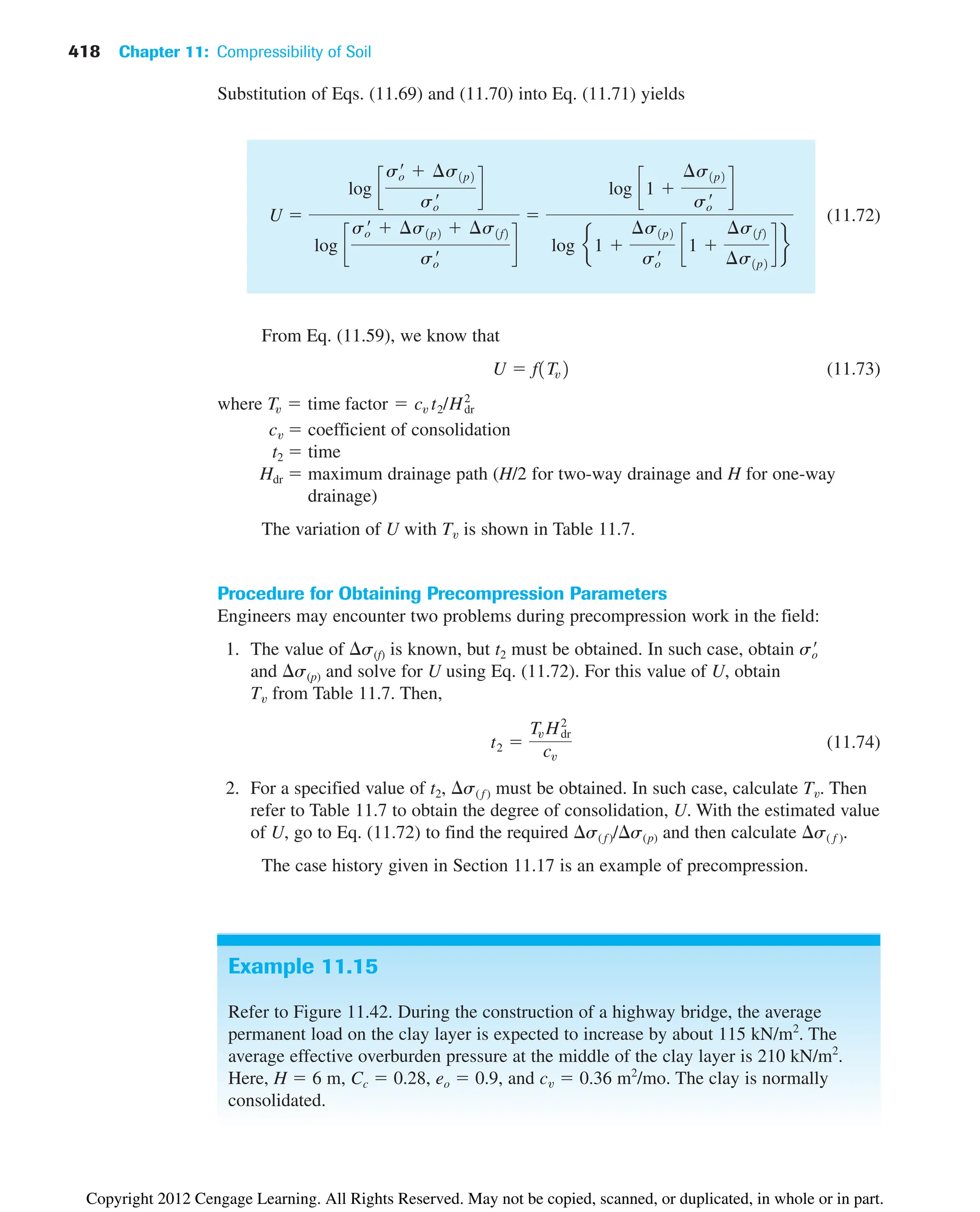
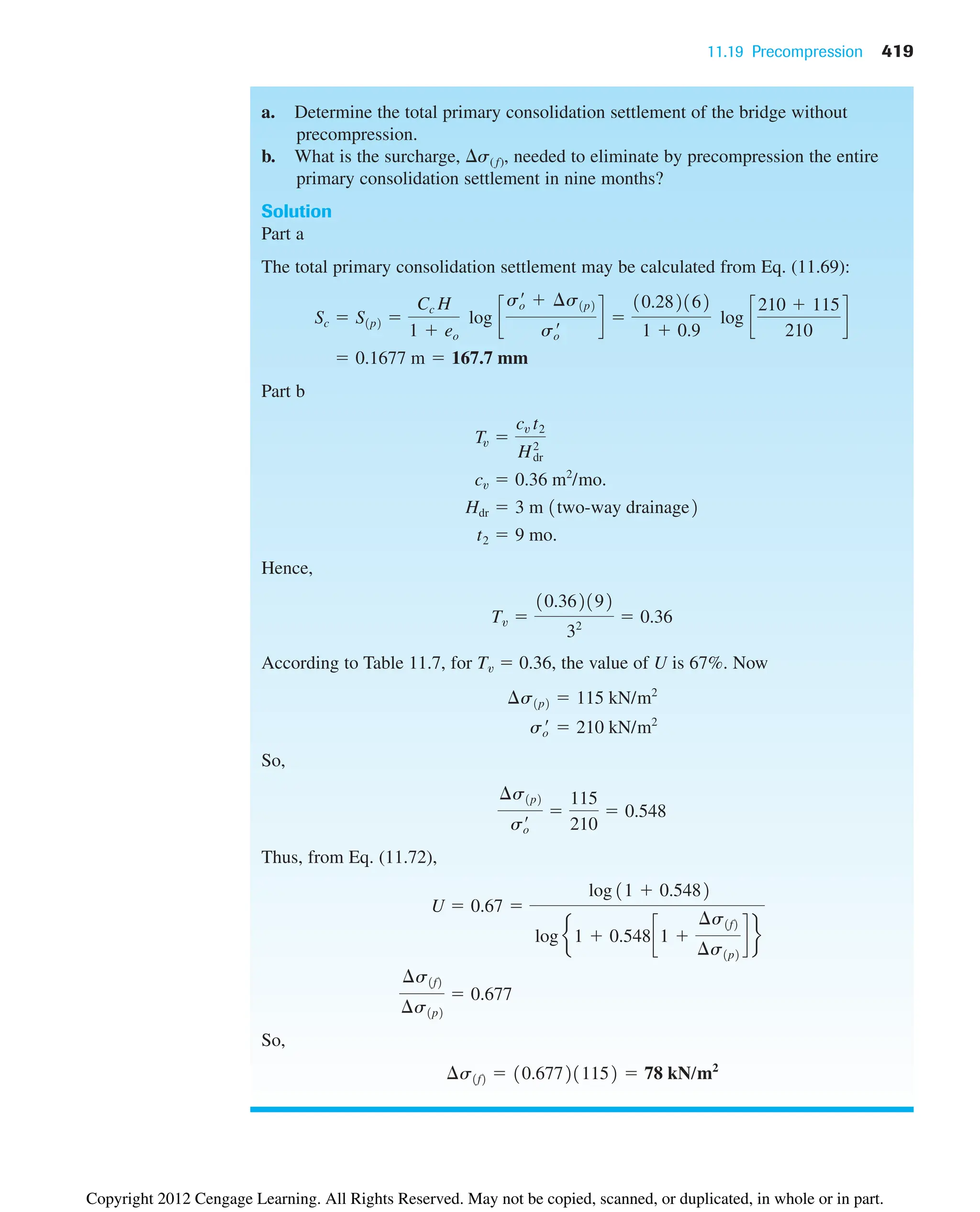
![420 Chapter 11: Compressibility of Soil
11.20 Summary and General Comments
This chapter discussed theories relating to the settlement of foundations. Following is a
summary of the topics covered.
• Total settlement of a foundation is the sum of elastic settlement and consolidation
settlement. Consolidation settlement has two components—primary and secondary.
• Elastic settlement (Section 11.3) is primarily a function of the size (length and width)
and rigidity of the foundation, the modulus of elasticity and Poisson’s ratio of the
soil supporting the foundation, and the intensity of the load applied.
• Consolidation is a time-dependent process of settlement of the saturated clay layer(s)
located below the groundwater table.
• Primary consolidation settlement can be calculated using Eqs. (11.29), (11.31),
and (11.32).
• Empirical relationships for compression index and swell index needed to estimate
primary consolidation settlement are given in Sections 11.11 and 11.12.
• Secondary consolidation settlement can be estimated using Eq. (11.42).
• The degree of consolidation at any time after load application is a function of the
nondimensional time factor Tv [see Table 11.7 and Eqs. (11.60)–(11.63)].
• The coefficient of consolidation for a given loading range can be obtained by using
logarithm-of-time, square-root-of-time, hyperbola, and early stage log-t methods
(Section 11.15).
• Sand drains and prefabricated vertical drains may be used to accelerate the consoli-
dation process in the field (Section 11.18).
• Precompression is a technique to reduce postconstruction settlement by application
of a temporary surcharge on the ground surface for a limited period of time. The
surcharge is removed when construction begins.
There are several case histories in the literature for which the fundamental principles
of soil compressibility have been used to predict and compare the actual total settlement
and the time rate of settlement of soil profiles under superimposed loading. In some cases,
the actual and predicted maximum settlements agree remarkably; in many others, the
predicted settlements deviate to a large extent from the actual settlements observed. The
disagreement in the latter cases may have several causes:
1. Improper evaluation of soil properties
2. Nonhomogeneity and irregularity of soil profiles
3. Error in the evaluation of the net stress increase with depth, which induces
settlement
The variation between the predicted and observed time rate of settlement may also
be due to
• Improper evaluation of cv (see Section 11.15)
• Presence of irregular sandy seams within the clay layer, which reduces the length of
the maximum drainage path, Hdr
Copyright 2012 Cengage Learning. All Rights Reserved. May not be copied, scanned, or duplicated, in whole or in part.](https://image.slidesharecdn.com/principlesofgeotechnicalengineering-8thedition-231222125509-7e44d9bf/75/Principles-of-Geotechnical-Engineering-8th-Edition-pdf-440-2048.jpg)
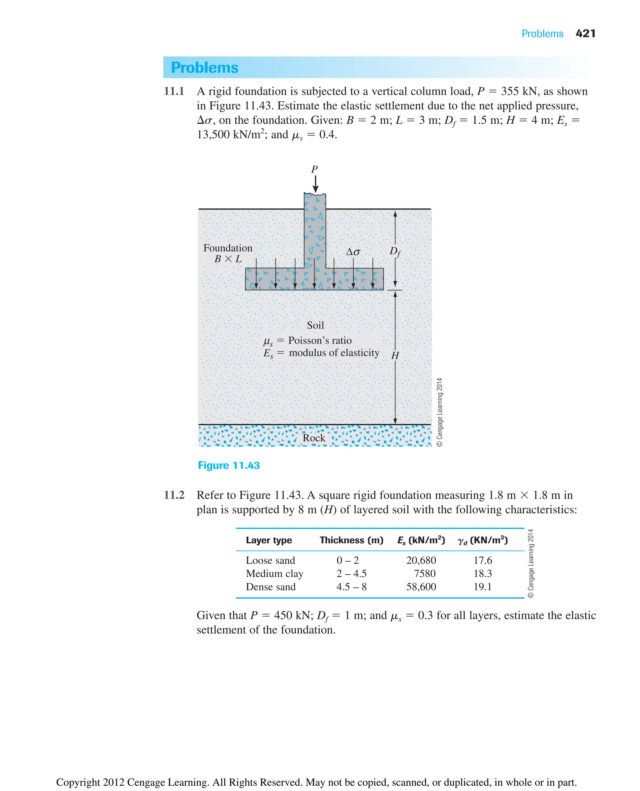
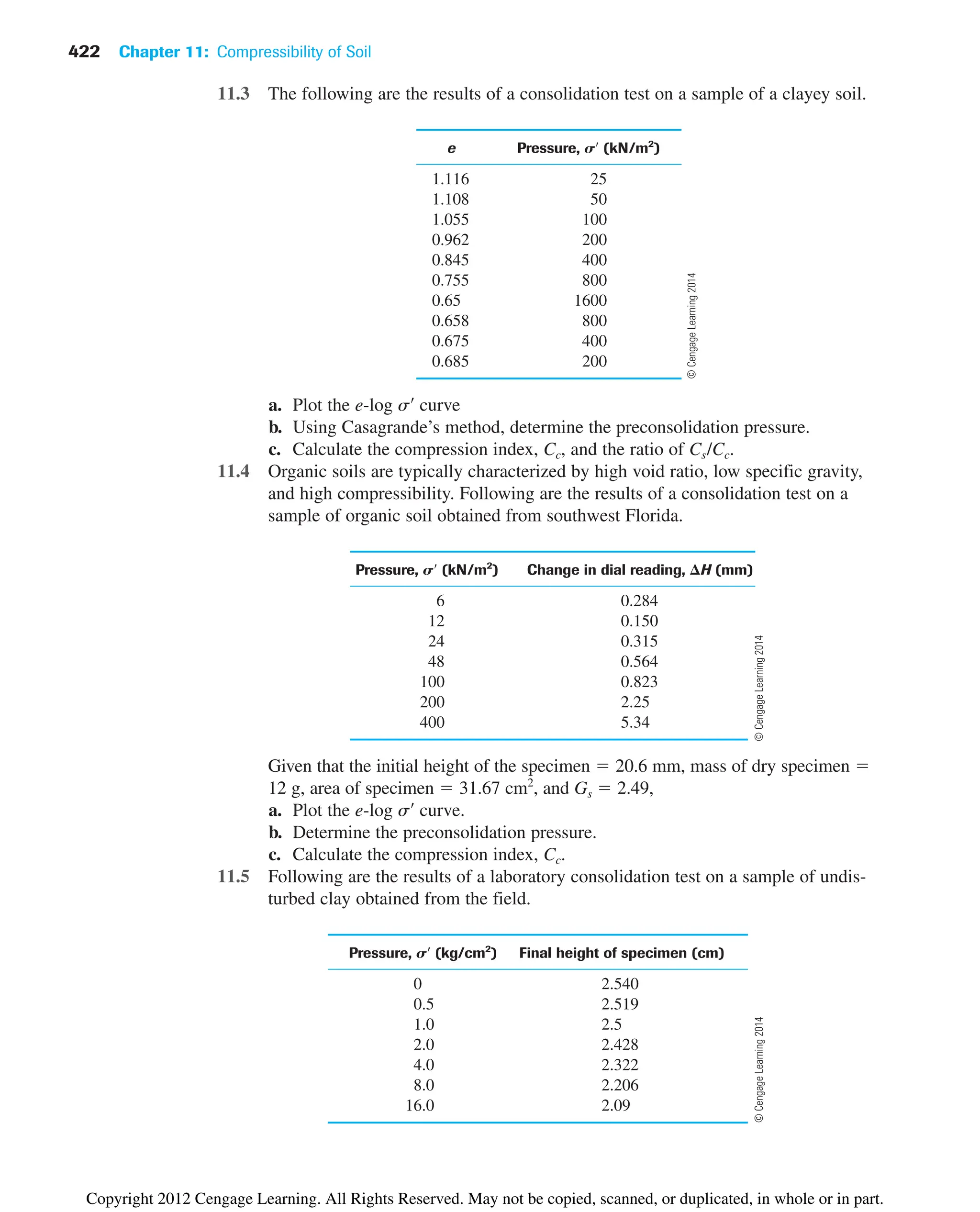
![The height of the specimen at the beginning of the test was 25.4 mm, and the diame-
ter was 63.5 mm. The moist specimen weighed 140 g and the water content was
determined to be 19%. Estimate the compression index and the preconsolidation
pressure from the e-log s¿ curve. Given: Gs 2.7.
11.6 Refer to Figure 11.43. Considering the soil to be a uniform clay layer, estimate
the primary consolidation settlement due to the foundation load. Given:
P 150 kN; B 3 m; L 3 m; Df 1.5 m; H 8 m; e 0.7; Gs 2.72; and
LL 42. Assume that the clay is normally consolidated, and the groundwater
table is at the foundation level. Use
11.7 Redo Problem 11.6 using the weighted average method [Eq. (11.68)] to calculate
the stress increase in the clay layer.
11.8 Consider the soil profile shown in Figure 11.44 subjected to the uniformly
distributed load, s, on the ground surface. Given: s 26 kN/m2
; H1 1.83 m;
H2 3.66 m; and H3 5.5 m. Soil characteristics are as follows:
• Sand: gd 17.9 kN/m3
; gsat 18.5 kN/m3
• Clay: gsat 18.3 kN/m3
; LL 38; e 0.73;
Estimate the primary consolidation settlement in the clay if
a. The clay is normally consolidated
b. The preconsolidation pressure
11.9 Refer to Figure 11.44. Estimate the primary consolidation settlement in the clay
layer. Given: s 85 kN/m2
; H1 2 m; H2 4 m; and H3 6 m. Soil charac-
teristics are as follows:
• Sand: e 0.65; Gs 2.66
• Clay: LL 54; e 0.98; Gs 2.74; ; Cs
1
6
Cc
sc
¿ 150 kN/m2
sc
¿ 105 kN/m2
Cs
1
5
Cc
¢s
P
BL
Problems 423
Sand
s
H1
H2
H3
Clay
Figure 11.44
©
Cengage
Learning
2014
Copyright 2012 Cengage Learning. All Rights Reserved. May not be copied, scanned, or duplicated, in whole or in part.](https://image.slidesharecdn.com/principlesofgeotechnicalengineering-8thedition-231222125509-7e44d9bf/75/Principles-of-Geotechnical-Engineering-8th-Edition-pdf-443-2048.jpg)
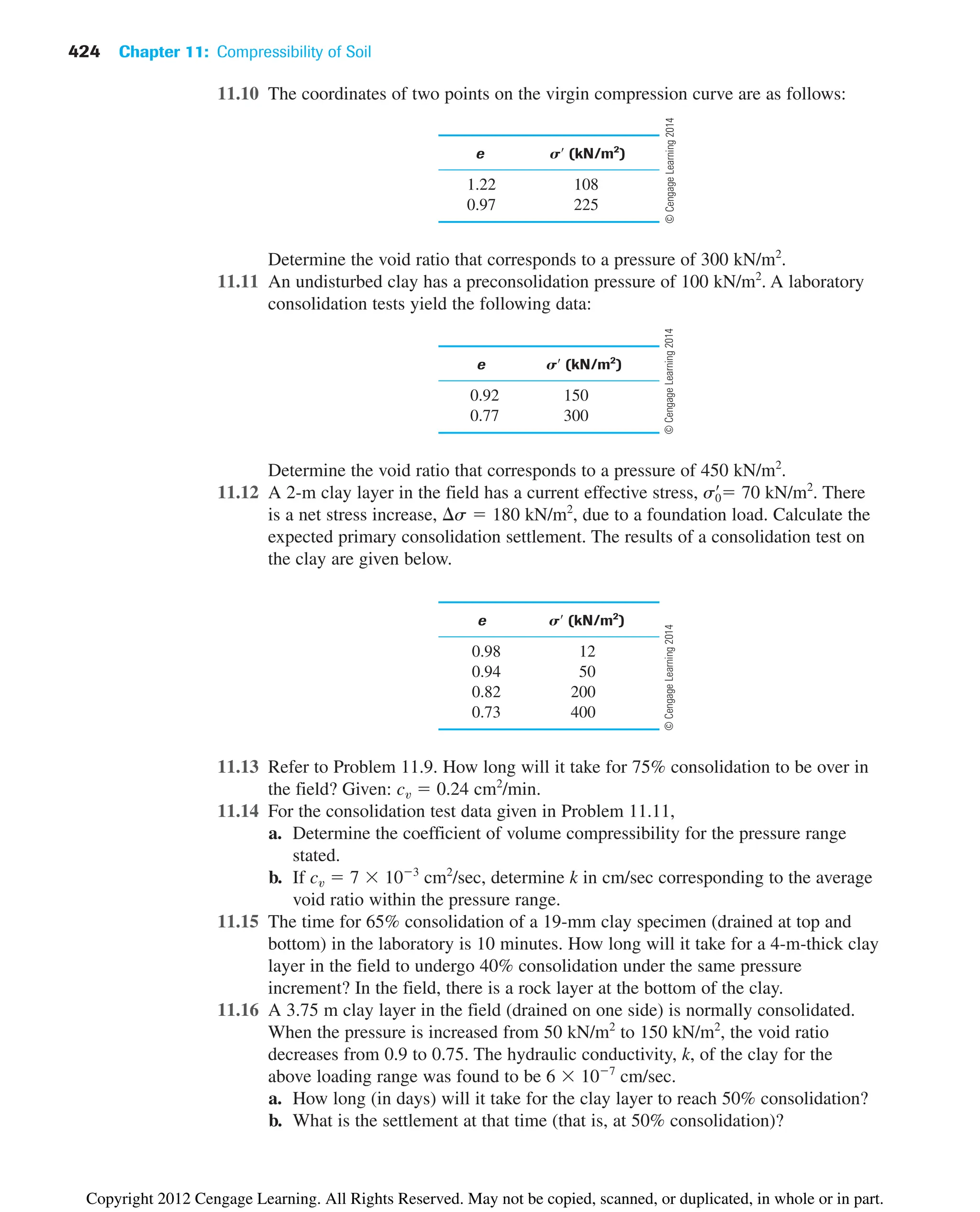
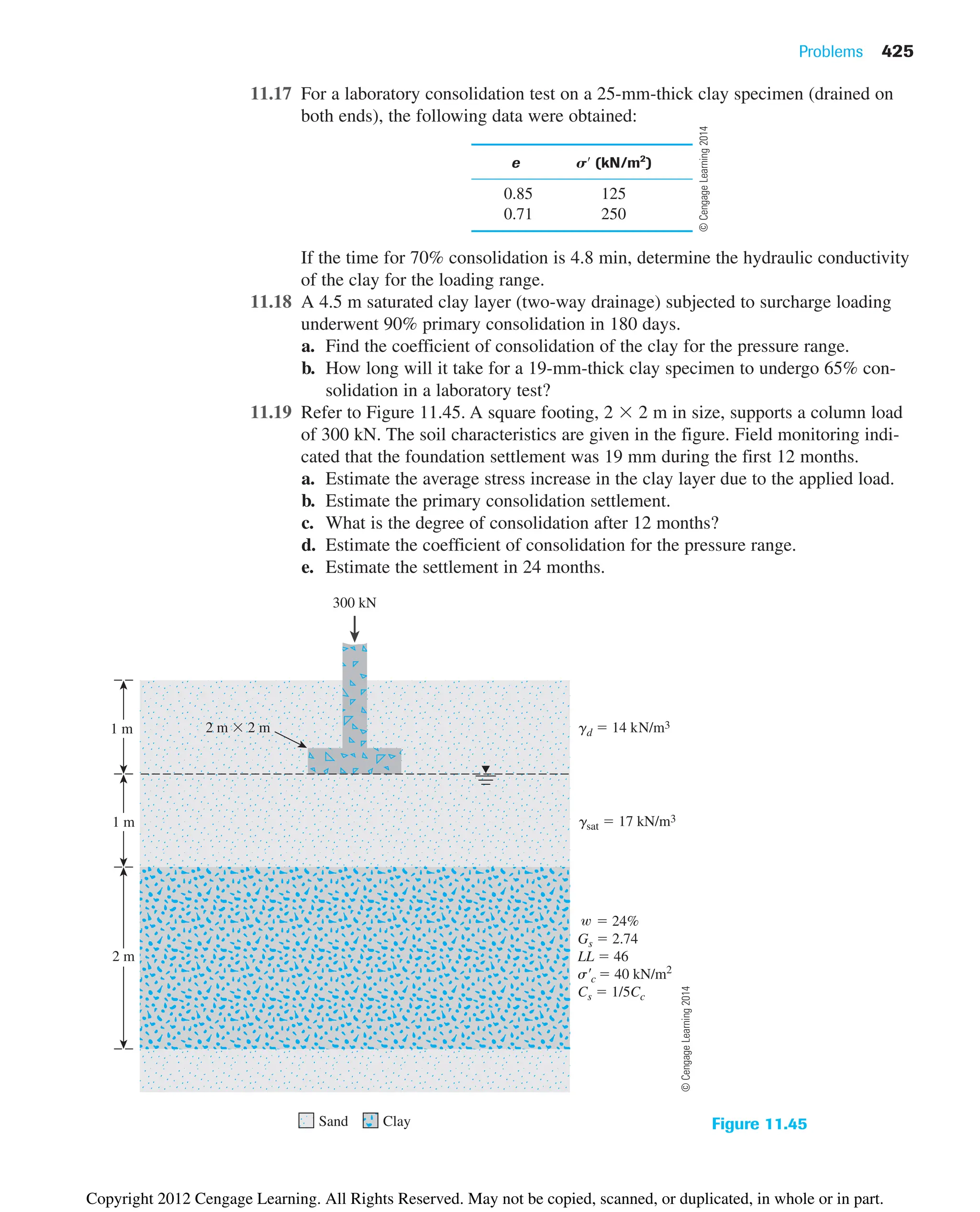
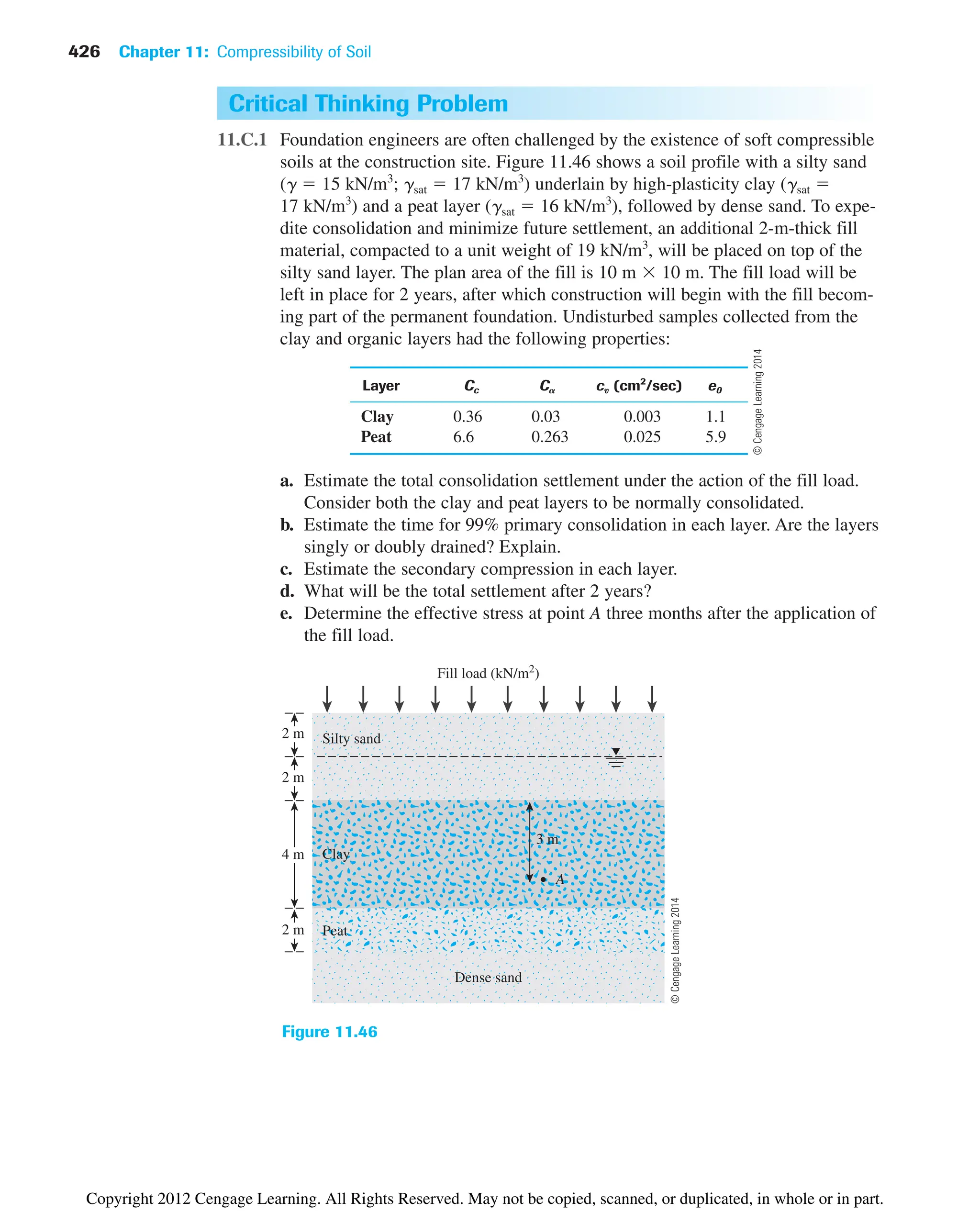
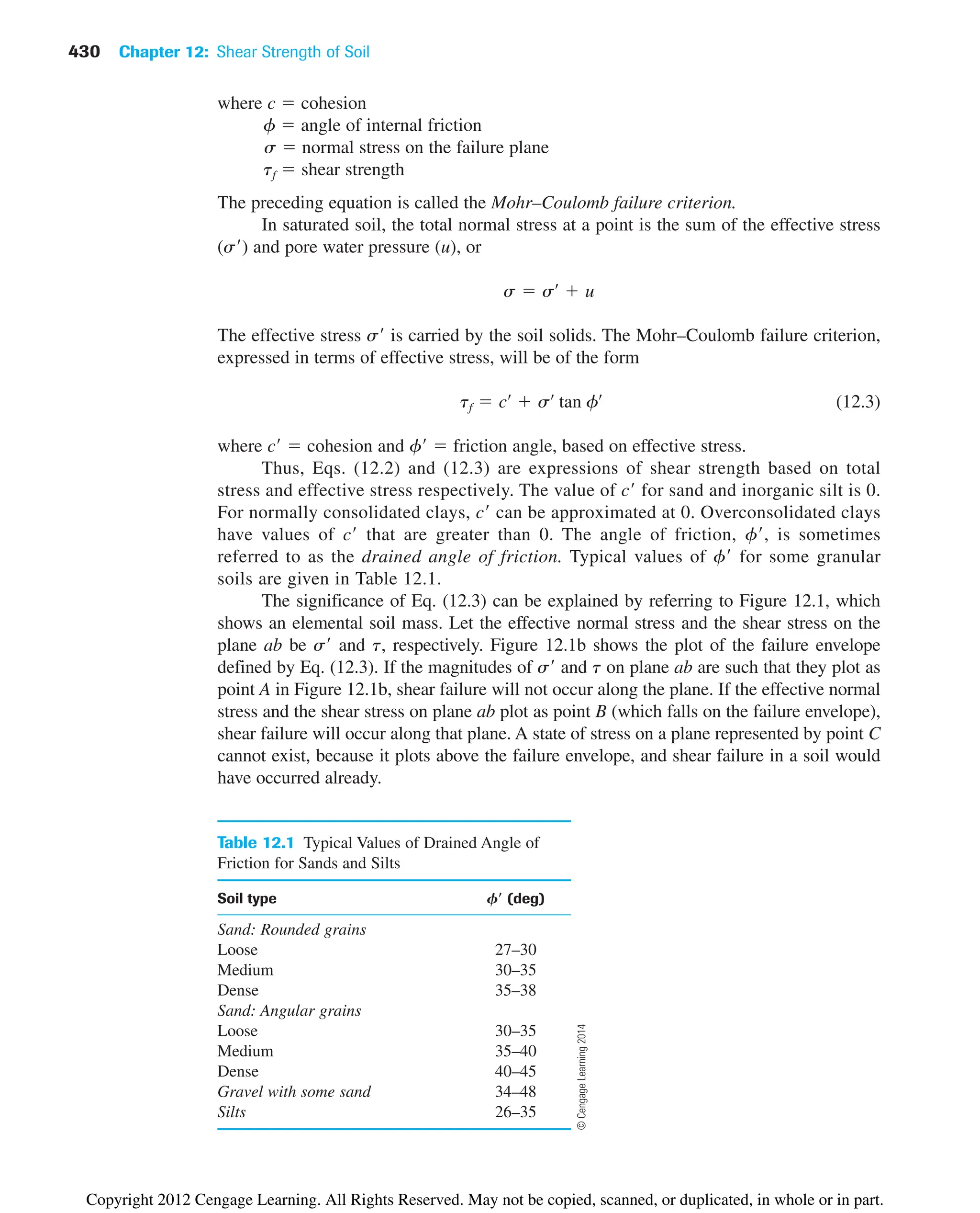
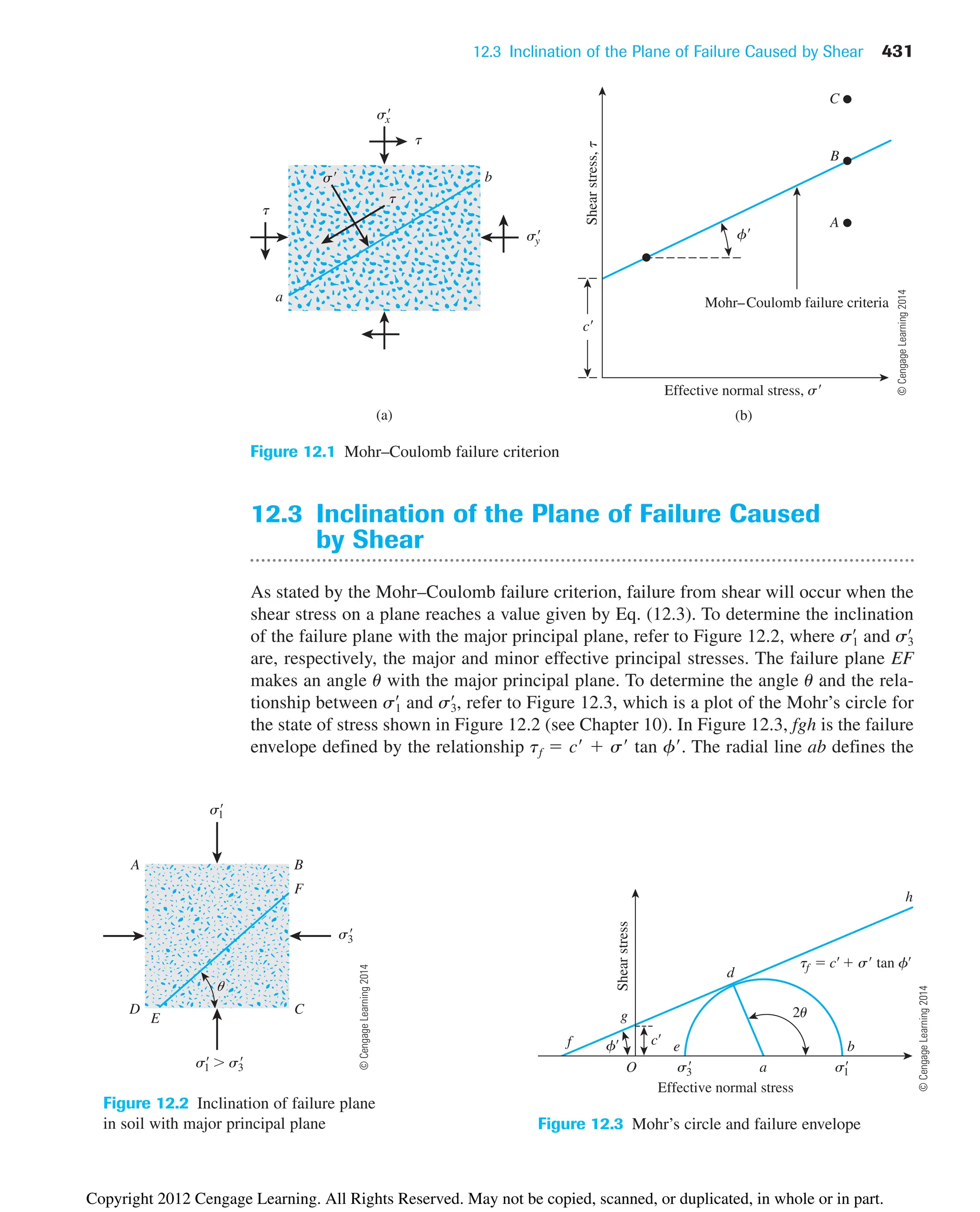
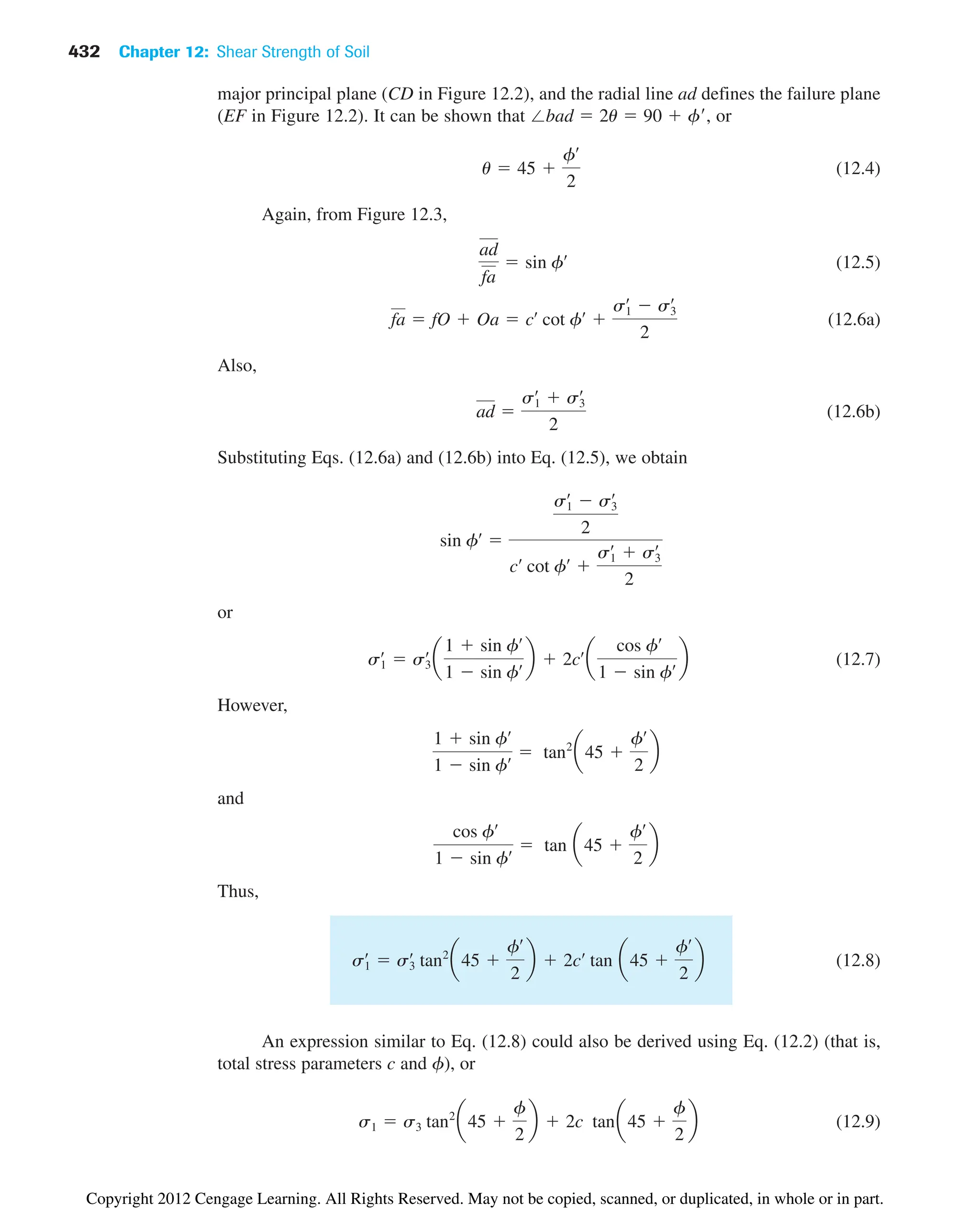
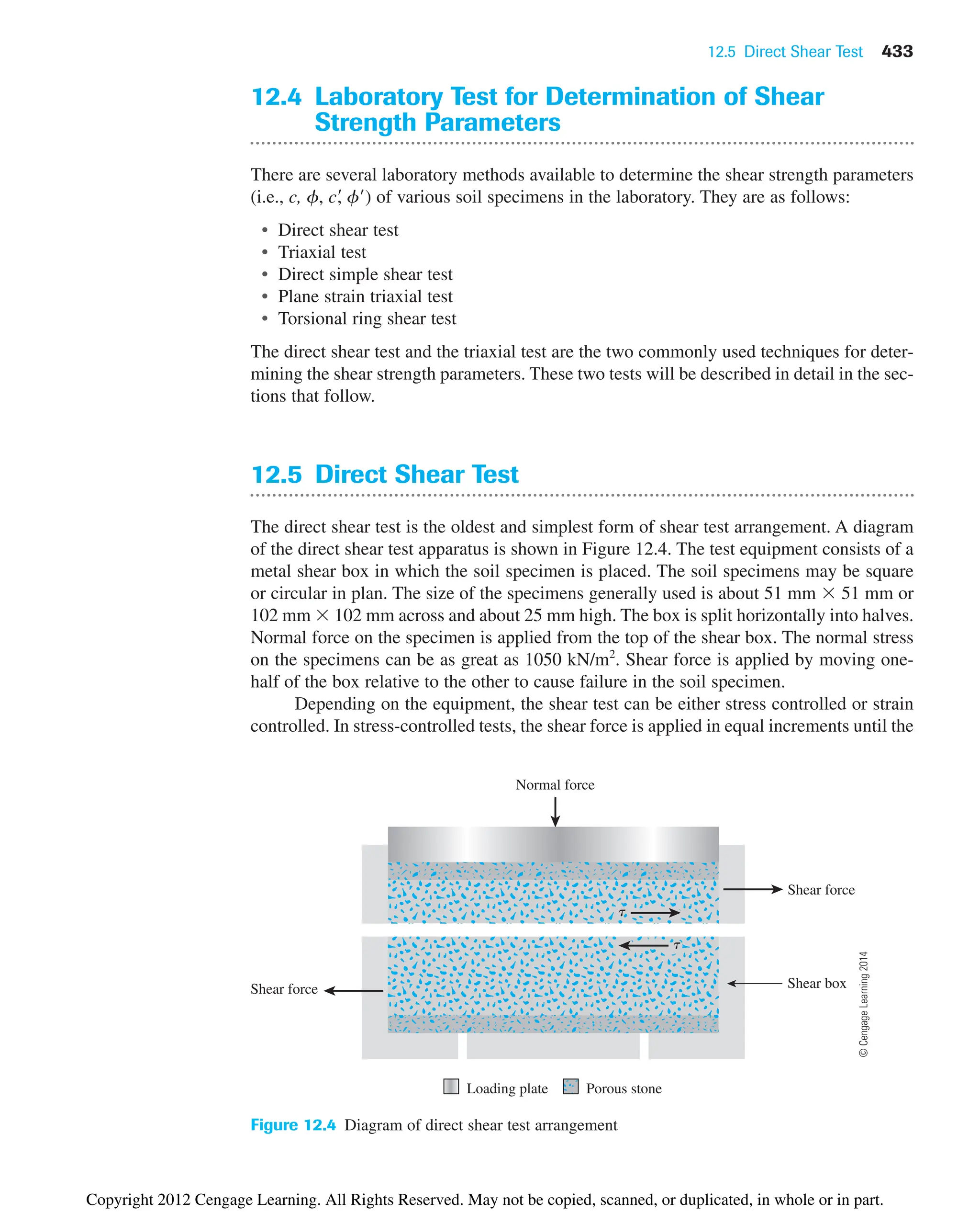
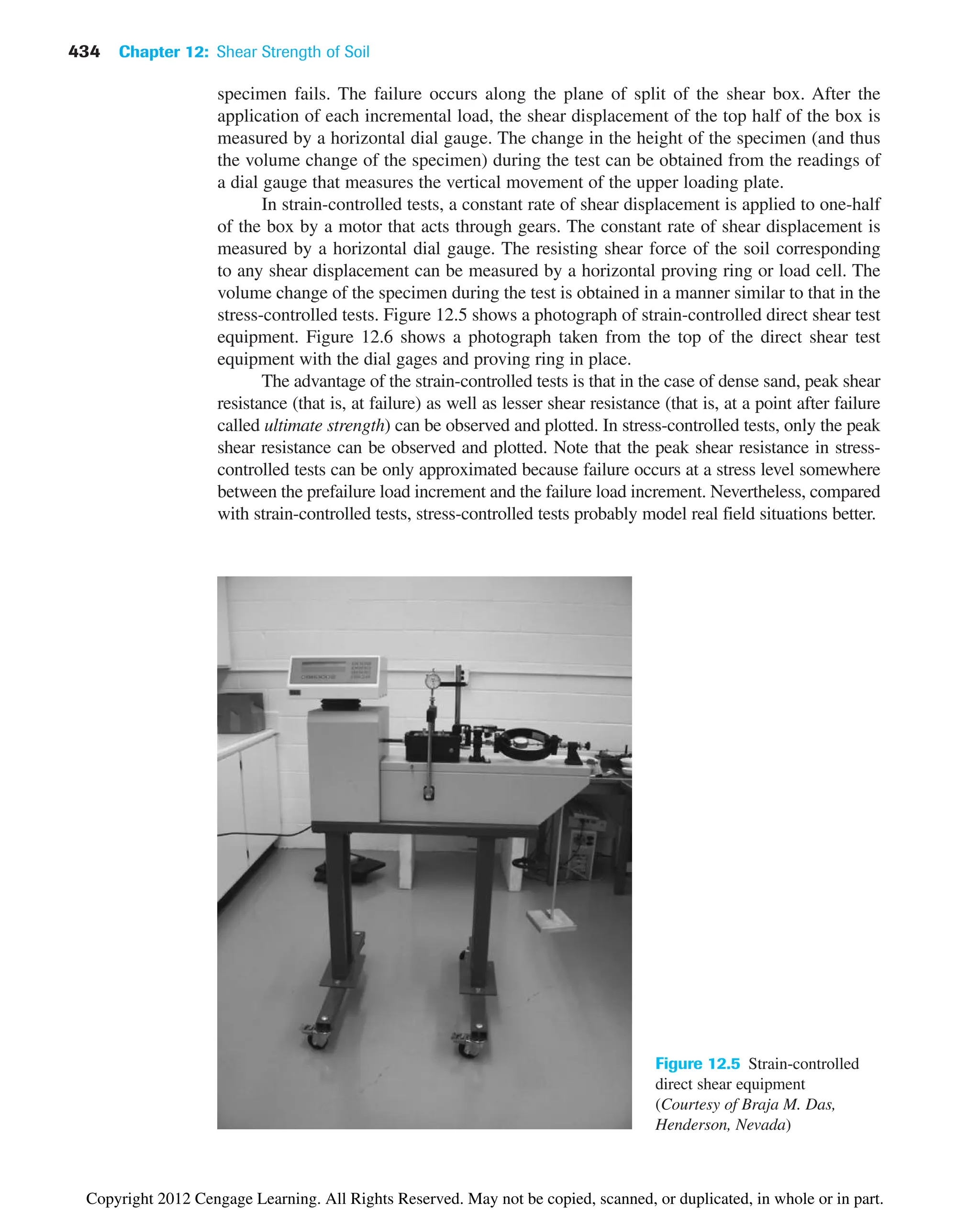

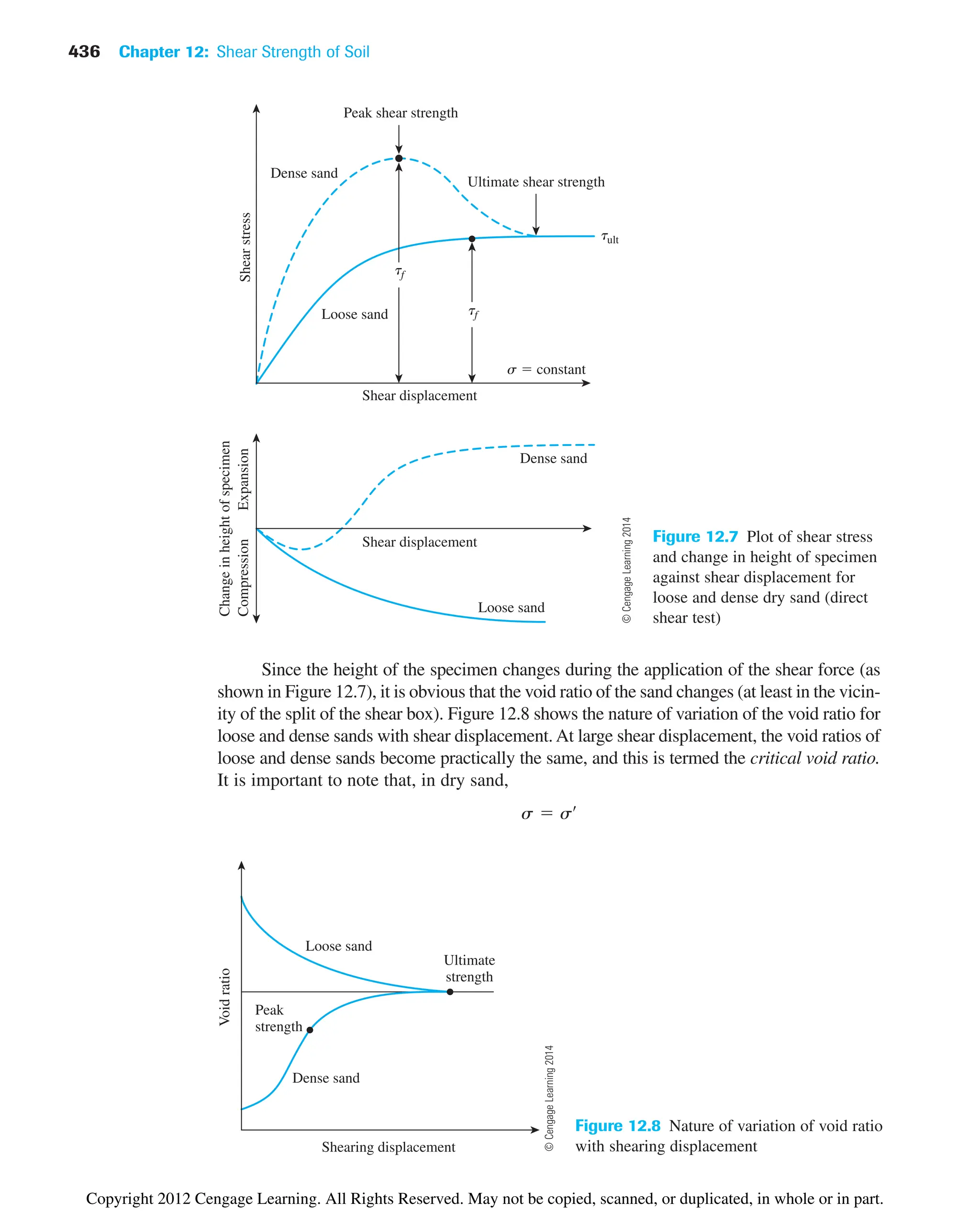
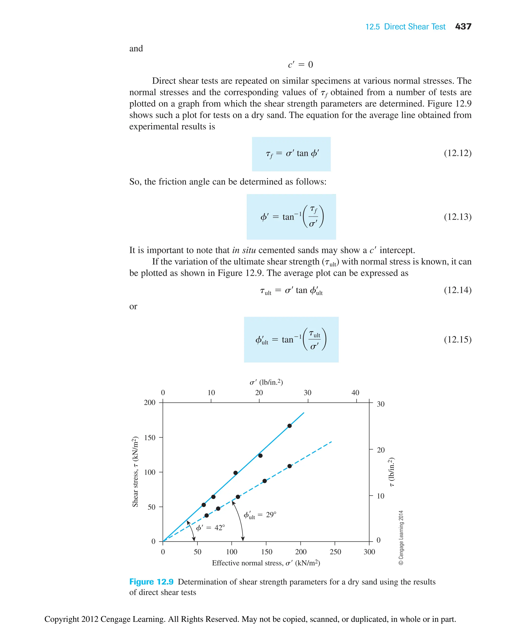
![438 Chapter 12: Shear Strength of Soil
12.6 Drained Direct Shear Test on Saturated
Sand and Clay
In the direct shear test arrangement, the shear box that contains the soil specimen is generally
kept inside a container that can be filled with water to saturate the specimen. A drained test
is made on a saturated soil specimen by keeping the rate of loading slow enough so that the
excess pore water pressure generated in the soil is dissipated completely by drainage. Pore
water from the specimen is drained through two porous stones. (See Figure 12.4.)
Because the hydraulic conductivity of sand is high, the excess pore water pressure
generated due to loading (normal and shear) is dissipated quickly. Hence, for an ordinary
loading rate, essentially full drainage conditions exist. The friction angle, f, obtained
from a drained direct shear test of saturated sand will be the same as that for a similar spec-
imen of dry sand.
The hydraulic conductivity of clay is very small compared with that of sand. When
a normal load is applied to a clay soil specimen, a sufficient length of time must elapse for
full consolidation—that is, for dissipation of excess pore water pressure. For this reason,
the shearing load must be applied very slowly. The test may last from two to five days.
Figure 12.10 shows the results of a drained direct shear test on an overconsolidated clay.
Figure 12.11 shows the plot of tf against s obtained from a number of drained direct shear
tests on a normally consolidated clay and an overconsolidated clay. Note that the value of
for a normally consolidated clay.
Similar to the ultimate shear strength in the case of sand (Figure 12.8), at large shear-
ing displacements, we can obtain the residual shear strength of clay (tr) in a drained test.
c¿ ⯝ 0
0
200
400
600
0 1 2 3 4
Horizontal deformation
Dimension of specimen in the direction of shear force
(%)
Residual shear strength
Shear
stress
(kN/m
2
)
Peak shear strength
Figure 12.10 Results of a drained direct shear test on an overconsolidated clay [Note: Residual
shear strength in clay is similar to ultimate shear strength in sand (see Figure 12.7)]
©
Cengage
Learning
2014
Copyright 2012 Cengage Learning. All Rights Reserved. May not be copied, scanned, or duplicated, in whole or in part.](https://image.slidesharecdn.com/principlesofgeotechnicalengineering-8thedition-231222125509-7e44d9bf/75/Principles-of-Geotechnical-Engineering-8th-Edition-pdf-458-2048.jpg)
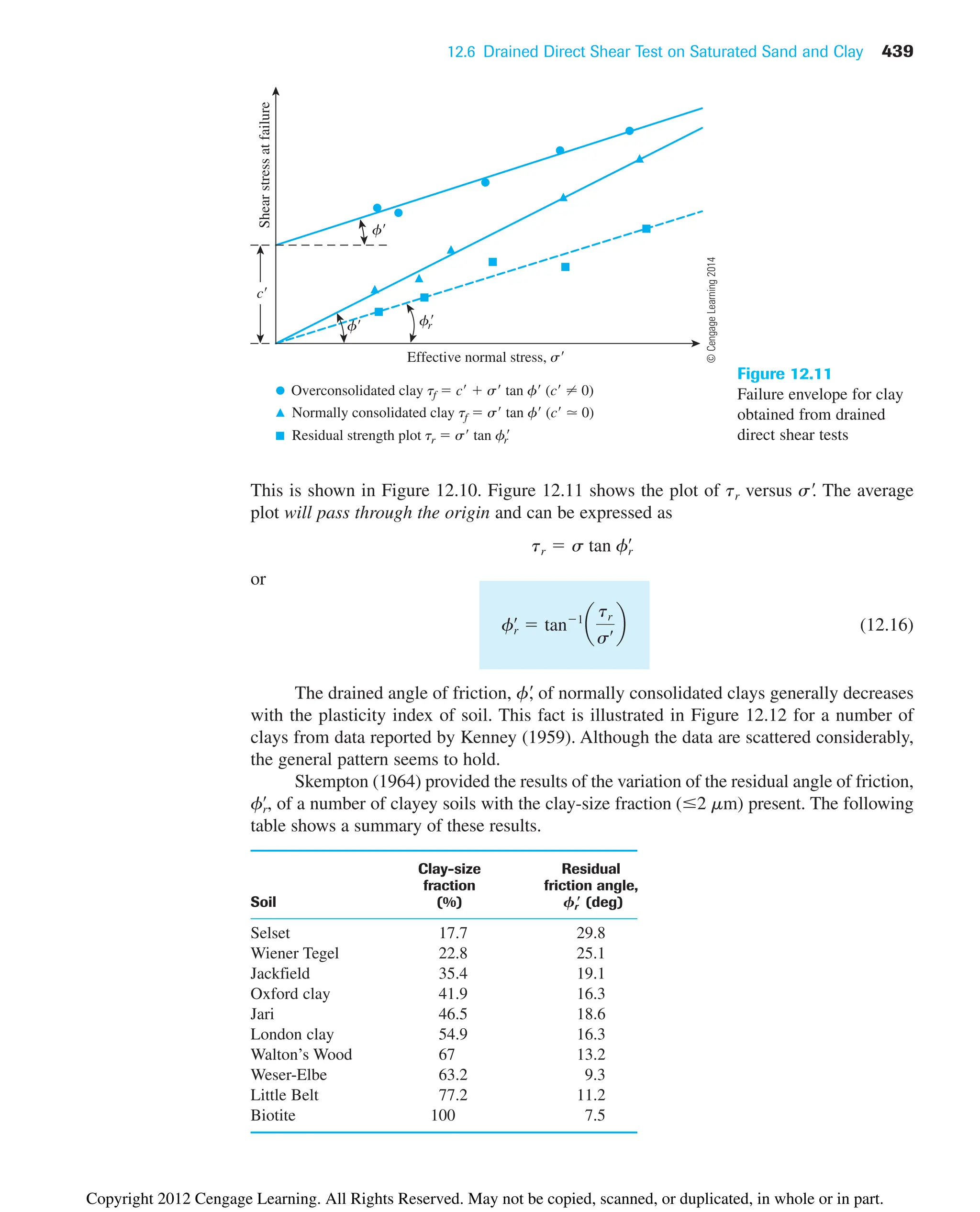
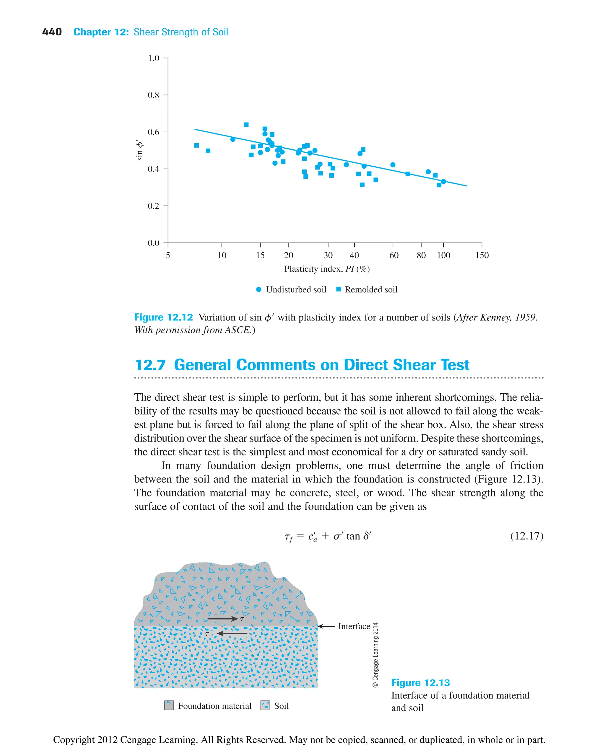
![12.7 General Comments on Direct Shear Test 441
where adhesion
d effective angle of friction between the soil and the foundation meterial
Note that the preceding equation is similar in form to Eq. (12.3). The shear strength
parameters between a soil and a foundation material can be conveniently determined by a
direct shear test. This is a great advantage of the direct shear test. The foundation material
can be placed in the bottom part of the direct shear test box and then the soil can be placed
above it (that is, in the top part of the box), as shown in Figure 12.14, and the test can be
conducted in the usual manner.
Figure 12.15 shows the results of direct shear tests conducted in this manner
with a quartz sand and concrete, wood, and steel as foundation materials, with
s 100 kN/m2
.
It was mentioned briefly in Section 12.1 [related to Eq. (12.1)] that Mohr’s failure
envelope is curvilinear in nature, and Eq. (12.2) is only an approximation. This fact should
be kept in mind when considering problems at higher confining pressures. Figure 12.16
shows the decrease of f and d with the increase of normal stress (s) for the same mate-
rials discussed in Figure 12.15. This can be explained by referring to Figure 12.17, which
shows a curved Mohr’s failure envelope. If a direct shear test is conducted with
the shear strength will be tf (1). So,
This is shown in Figure 12.17. In a similar manner, if the test is conducted with
, then
As can be seen from Figure 12.17, . Keeping this in mind, it must
be realized that the values of f given in Table 12.1 are only the average values.
d2
œ
d1
œ
since s2
œ
s112
œ
dœ
d2
œ
tan1
c
tf122
s122
œ d
sœ
s122
œ
d1
œ
tan1
c
tf112
s112
œ d
sœ
s112
œ
,
ca
œ
Shear
force
Normal force
Soil Foundation material
Figure 12.14 Direct shear test to determine interface friction angle
©
Cengage
Learning
2014
Copyright 2012 Cengage Learning. All Rights Reserved. May not be copied, scanned, or duplicated, in whole or in part.](https://image.slidesharecdn.com/principlesofgeotechnicalengineering-8thedition-231222125509-7e44d9bf/75/Principles-of-Geotechnical-Engineering-8th-Edition-pdf-461-2048.jpg)
![442 Chapter 12: Shear Strength of Soil
1/e
2.0
tan
(f
or
d)
1.2
Relative density, Dr (%)
0
25
50
75
100
1.9 1.8 1.7 1.6 1.5 1.4 1.3
1.0
0.8
0.6
0.4
0.2
0.0
Sand Wood Steel
Normal stress s 100 kN/m2
emin 0.51 emax 0.716
Concrete
Figure 12.15 Variation of tan f and tan d with 1/e
[Note: e void ratio, s 100 kN/m2
, quartz sand]
(After Acar, Durgunoglu, and Tumay, 1982. With
permission from ASCE.)
0.5 1.0 2.0 4.0 6.0 8.0 10
50
40
30
20
10
0
Friction
angle,
d
or
f
()
Sand Wood Steel
Concrete
Normal stress, s ( 102 kN/m2)
Figure 12.16 Variation of f and d with s
(Note: Relative density 45%; quartz sand) (After Acar,
Durgunoglu, and Tumay, 1982. With permission
from ASCE.)
d1
d2
[tf(1), s(1)]
[tf(2), s(2)]
Mohr’s failure envelope in sand
Shear
stress,
t
Normal stress, s
Figure 12.17
Curvilinear nature of Mohr’s
failure envelope in sand
©
Cengage
Learning
2014
Copyright 2012 Cengage Learning. All Rights Reserved. May not be copied, scanned, or duplicated, in whole or in part.](https://image.slidesharecdn.com/principlesofgeotechnicalengineering-8thedition-231222125509-7e44d9bf/75/Principles-of-Geotechnical-Engineering-8th-Edition-pdf-462-2048.jpg)
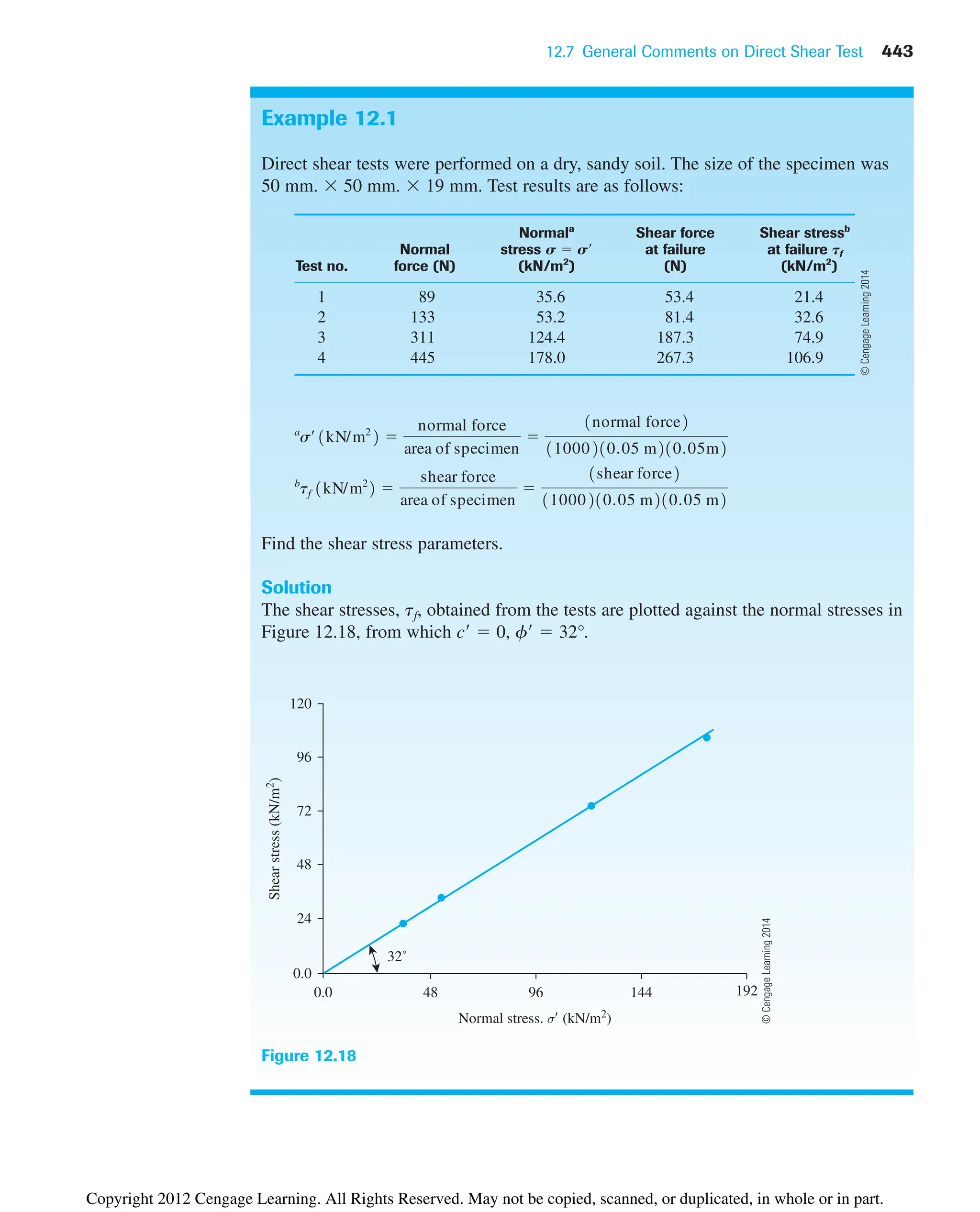
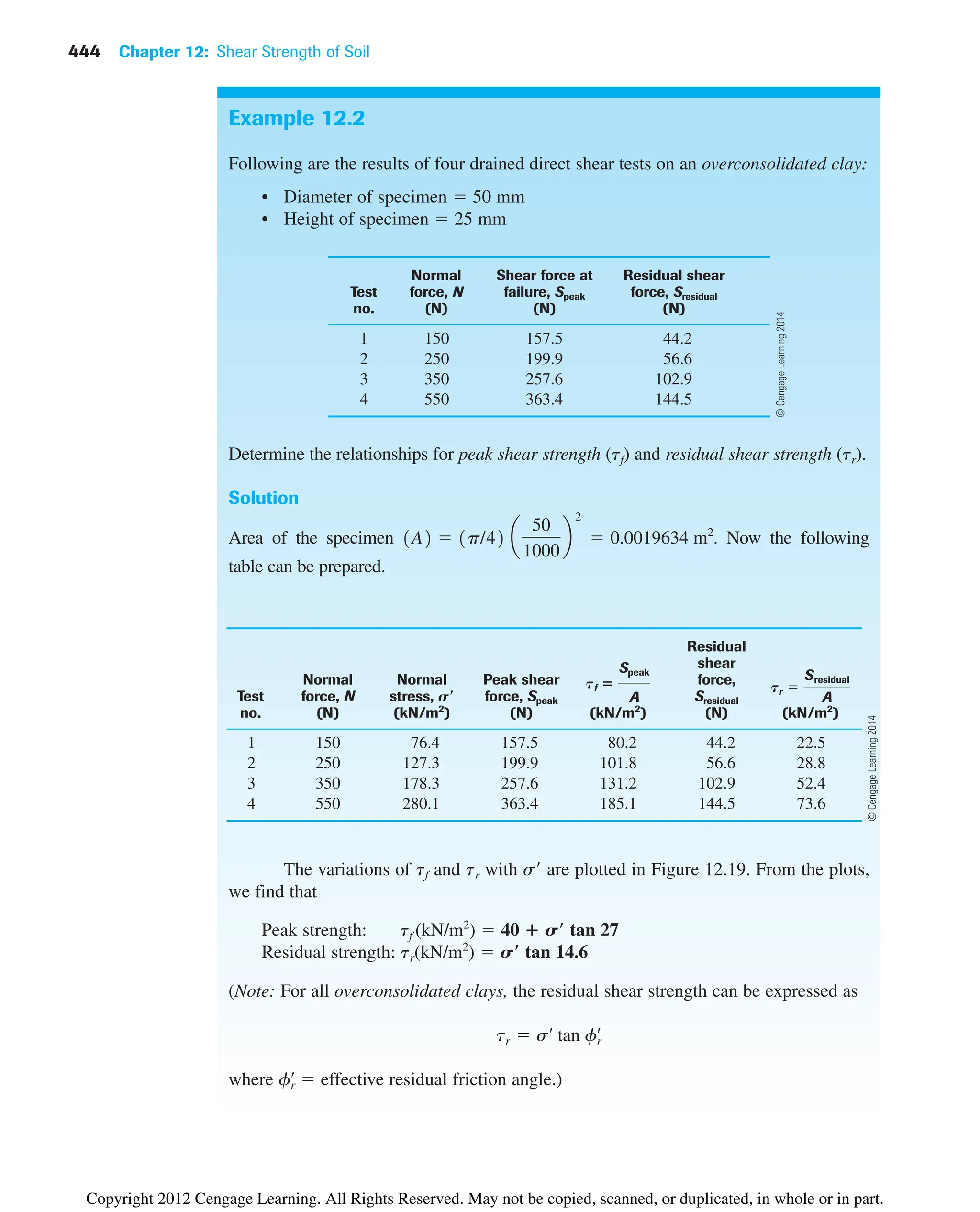
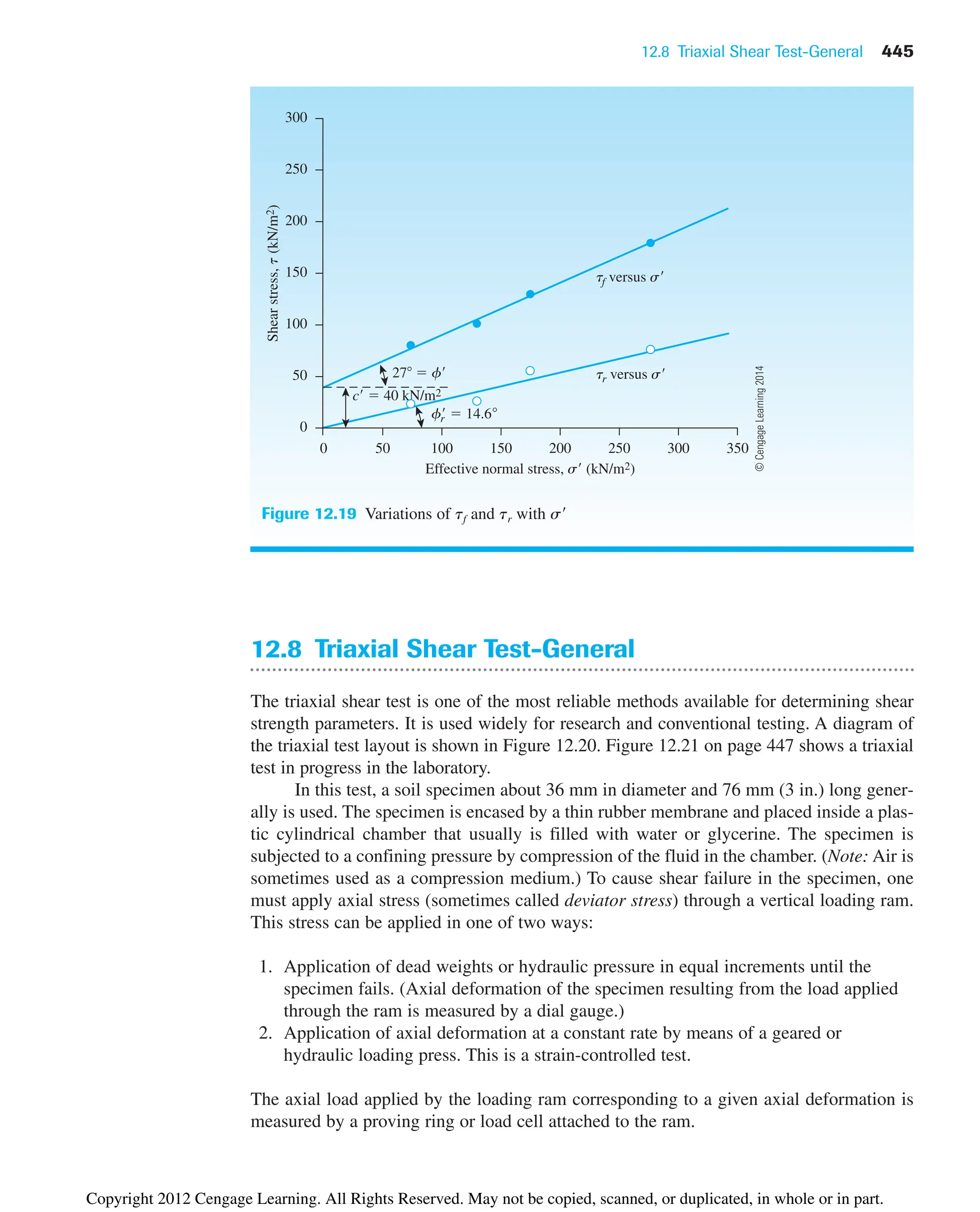
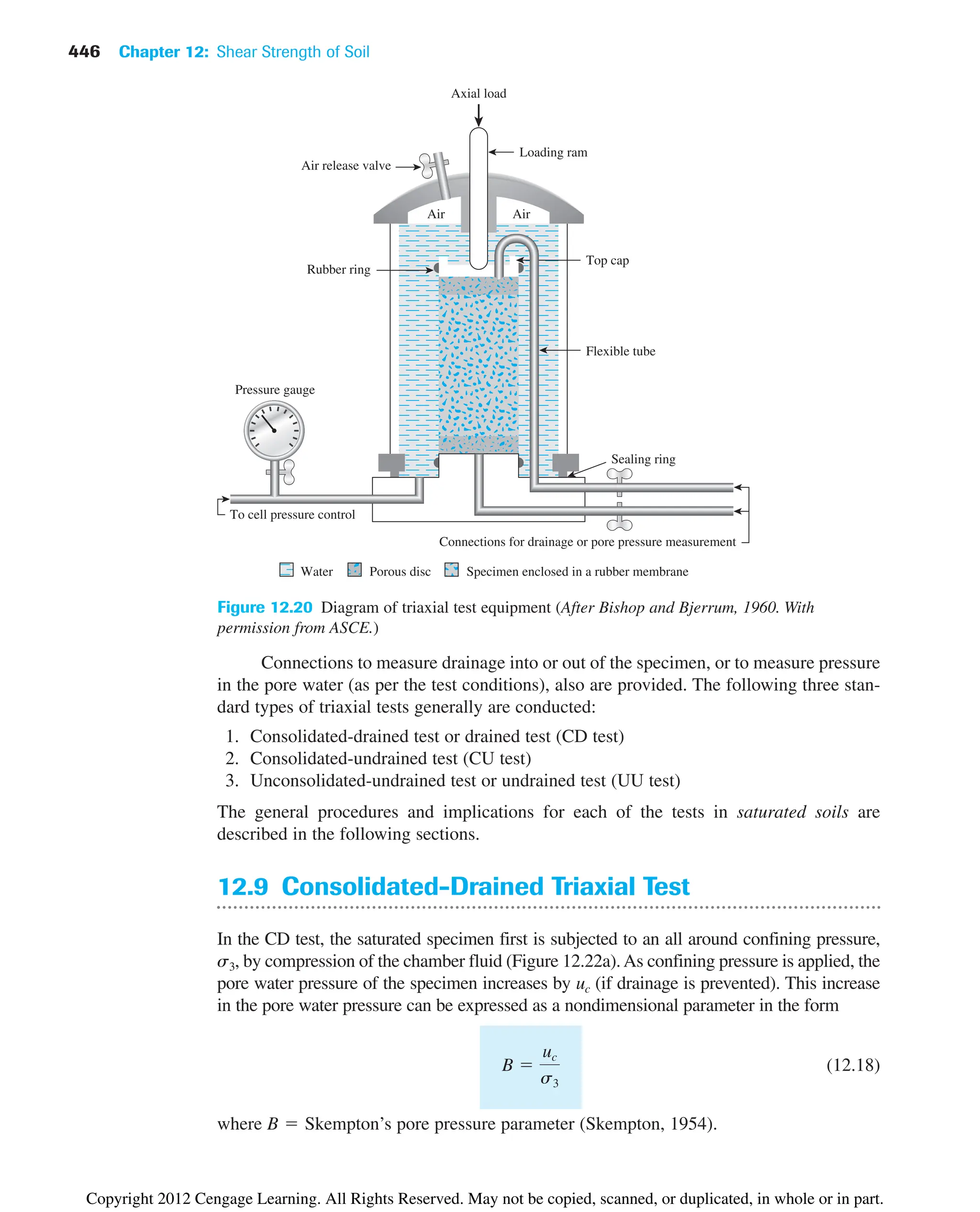
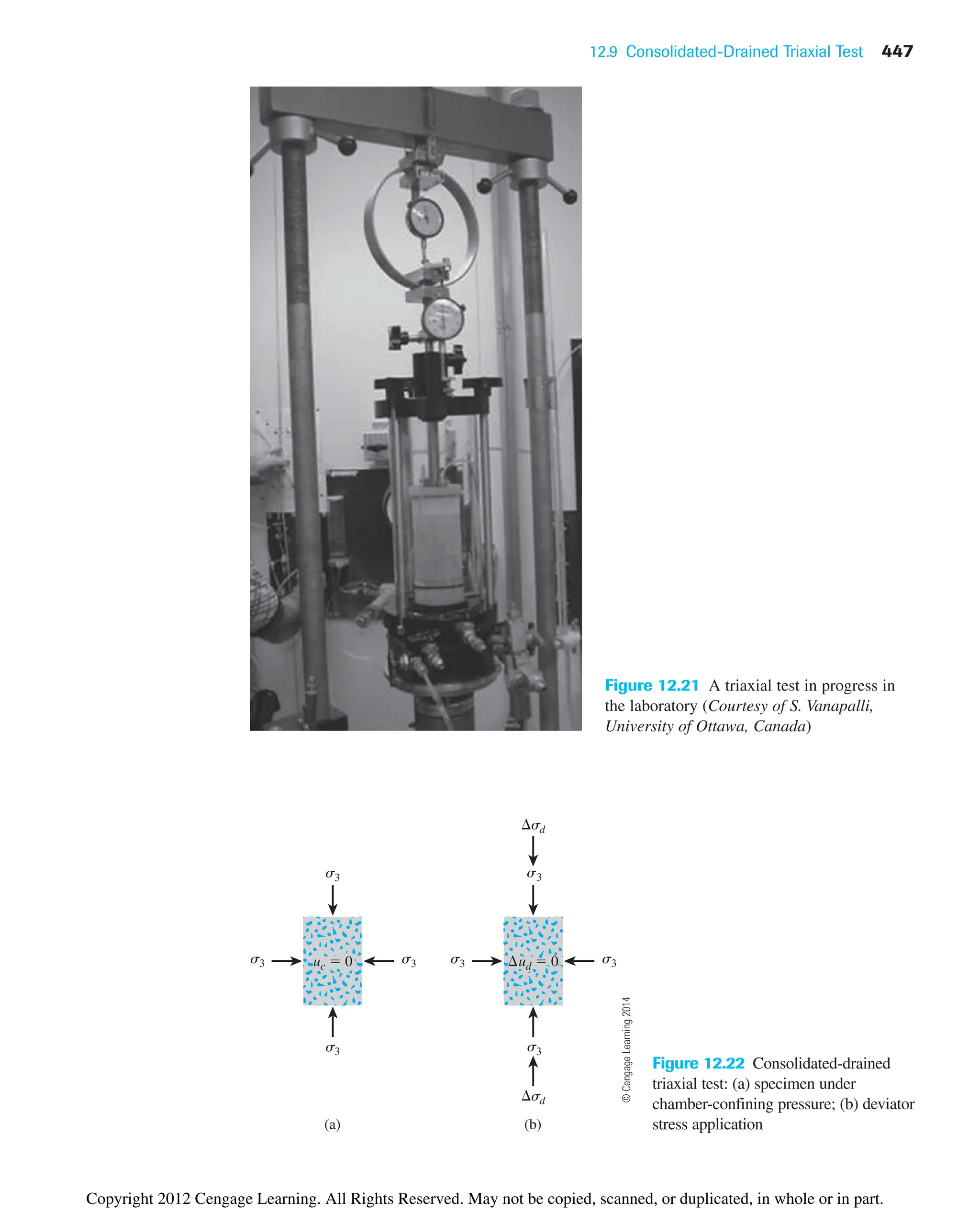
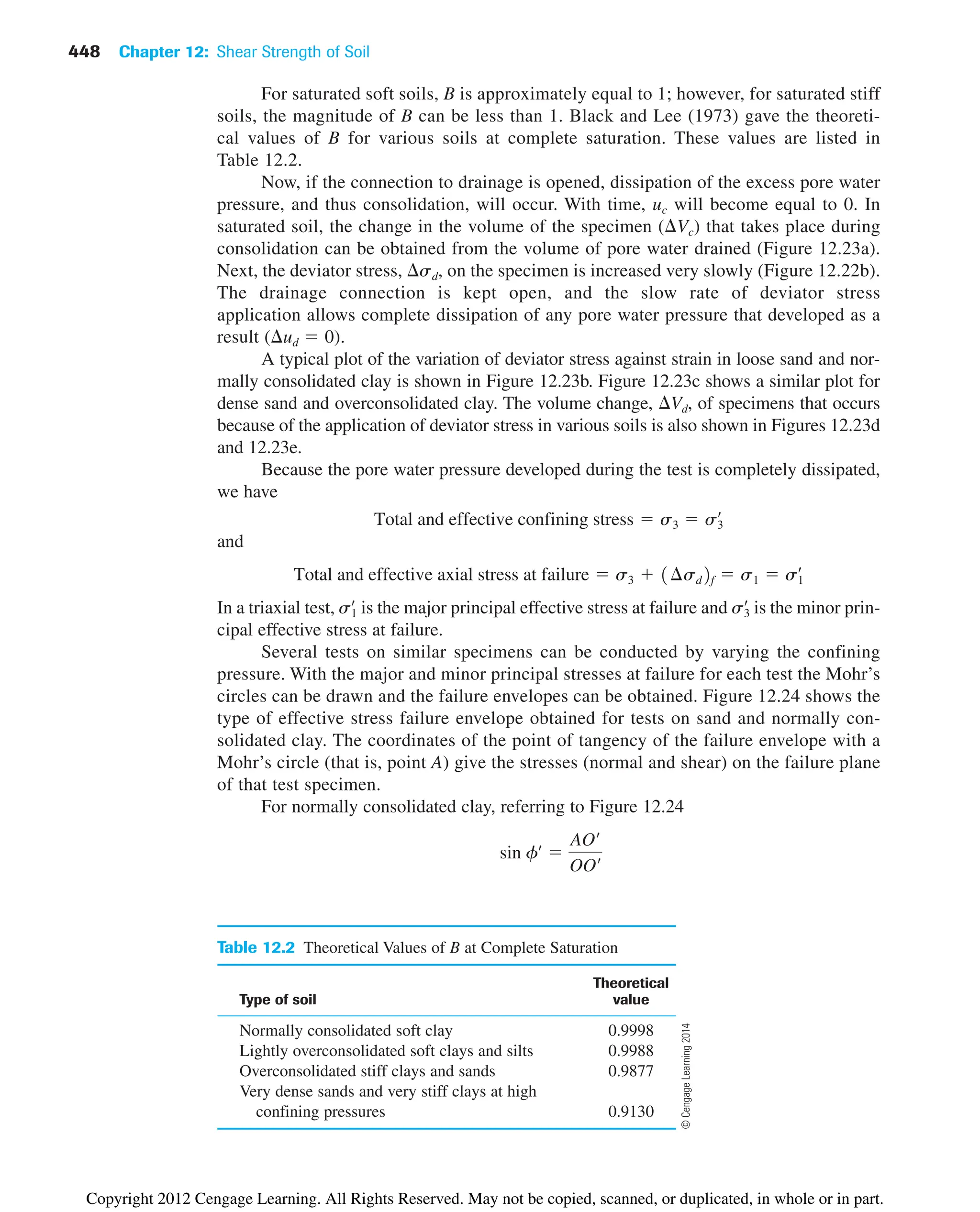
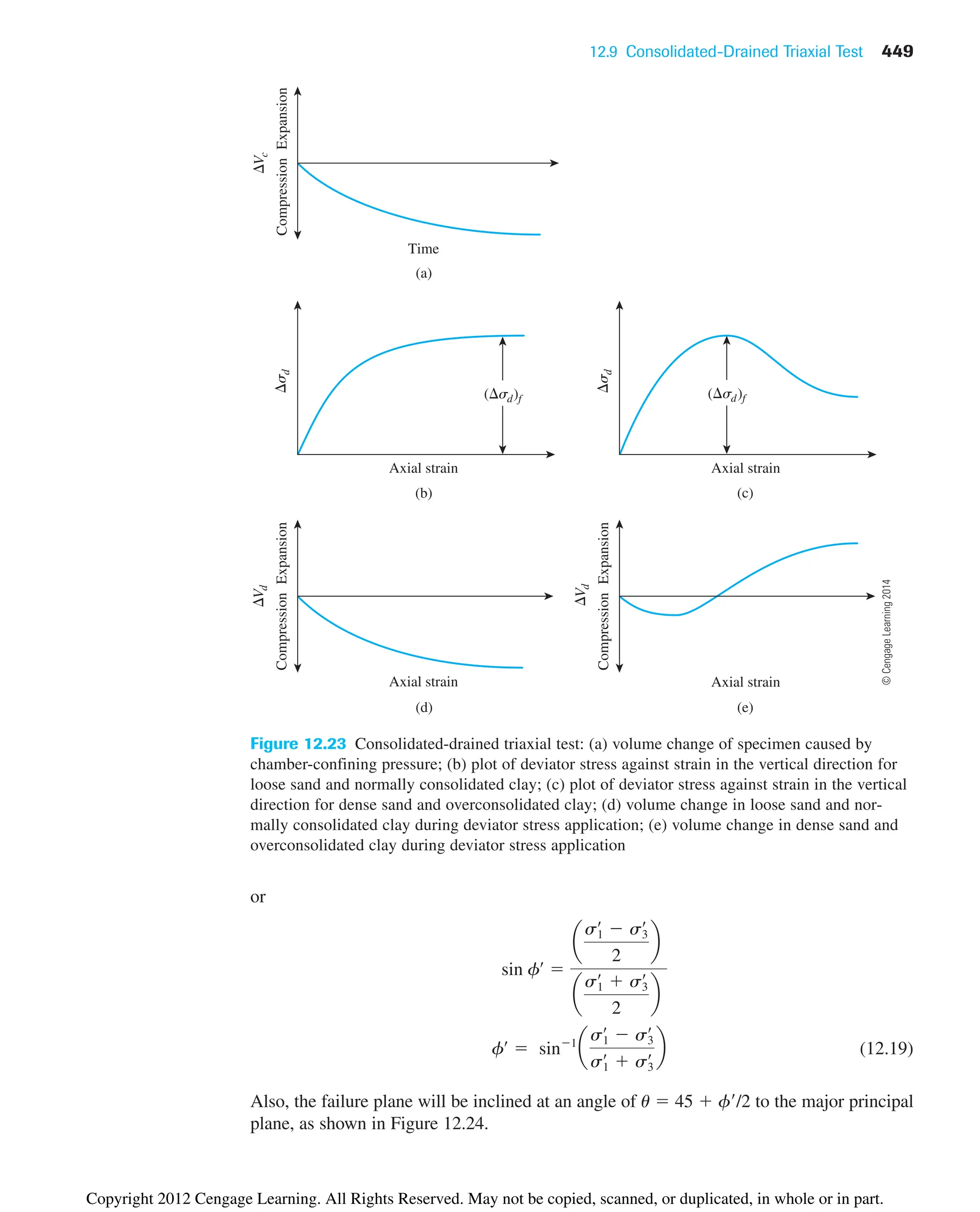
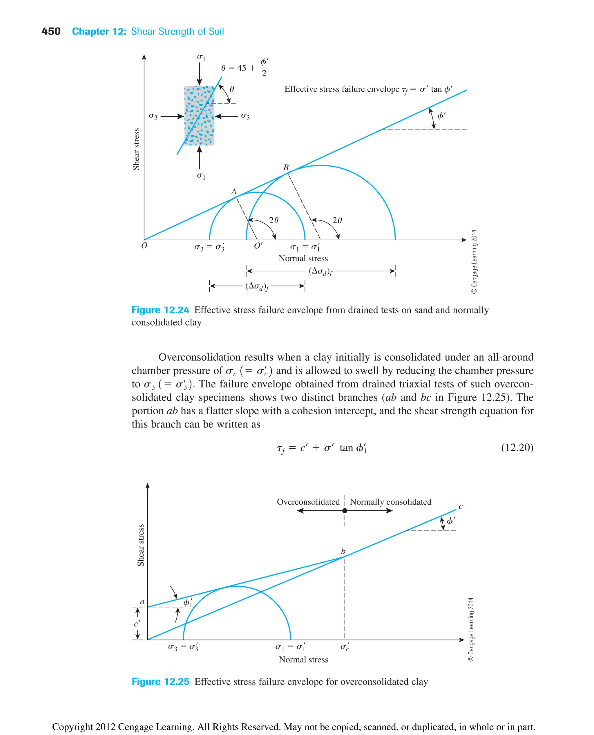

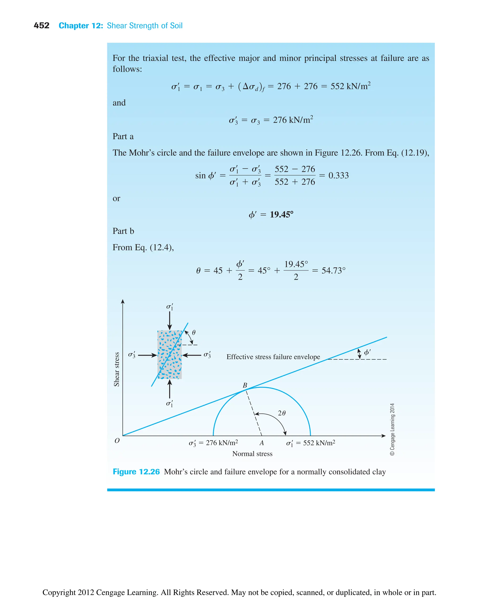
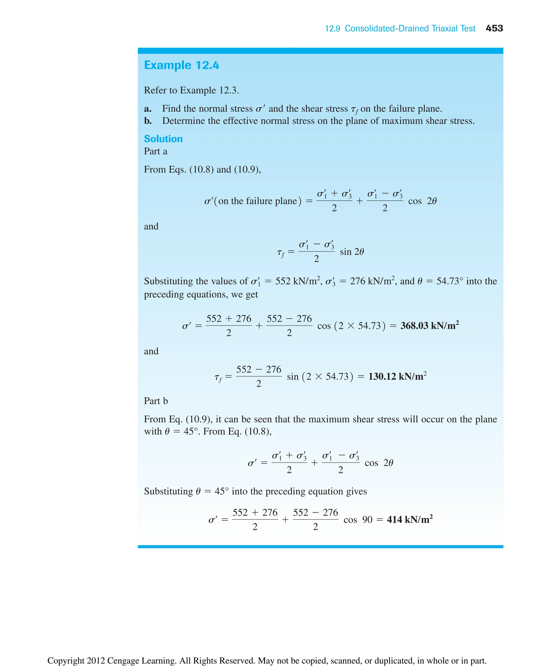
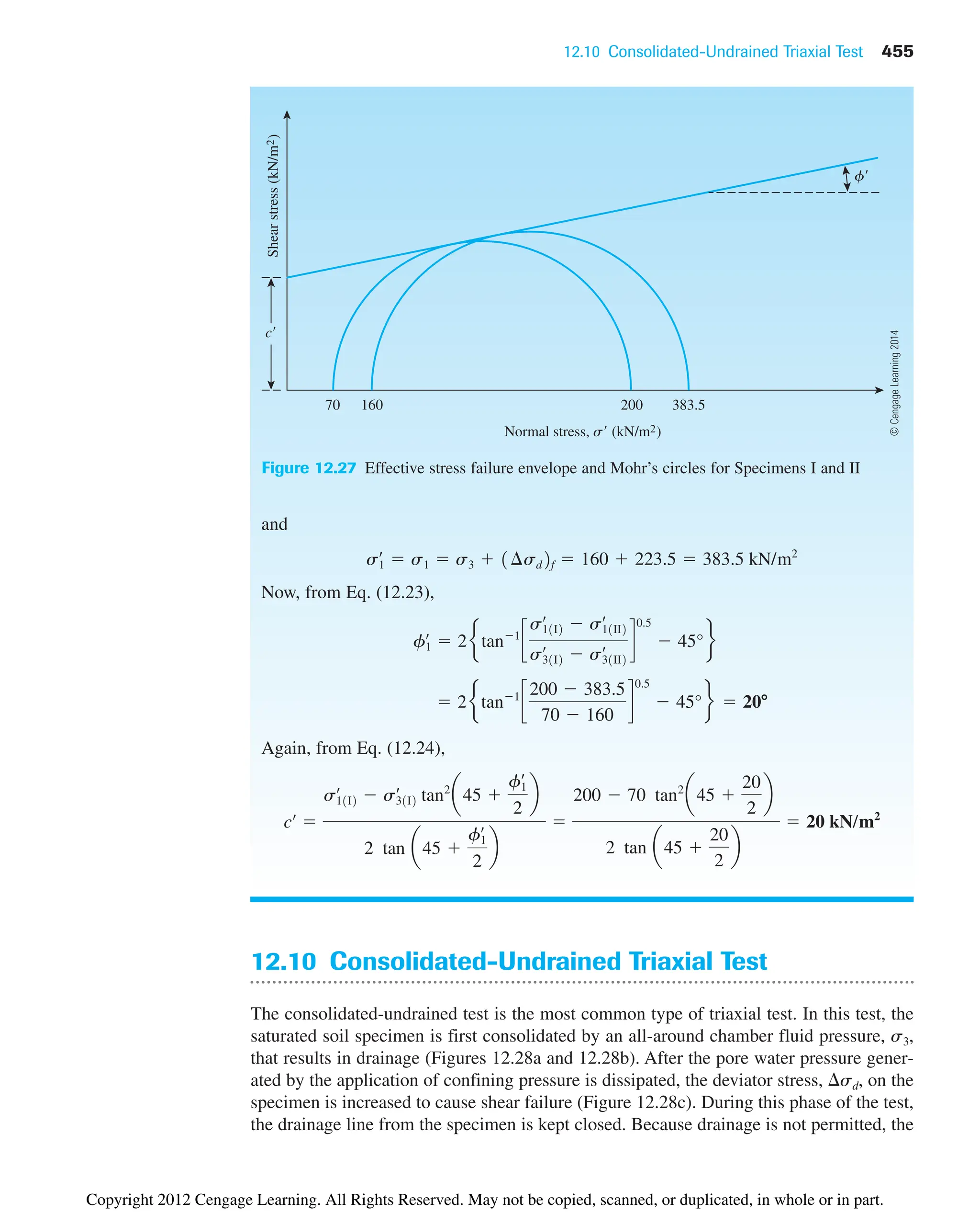
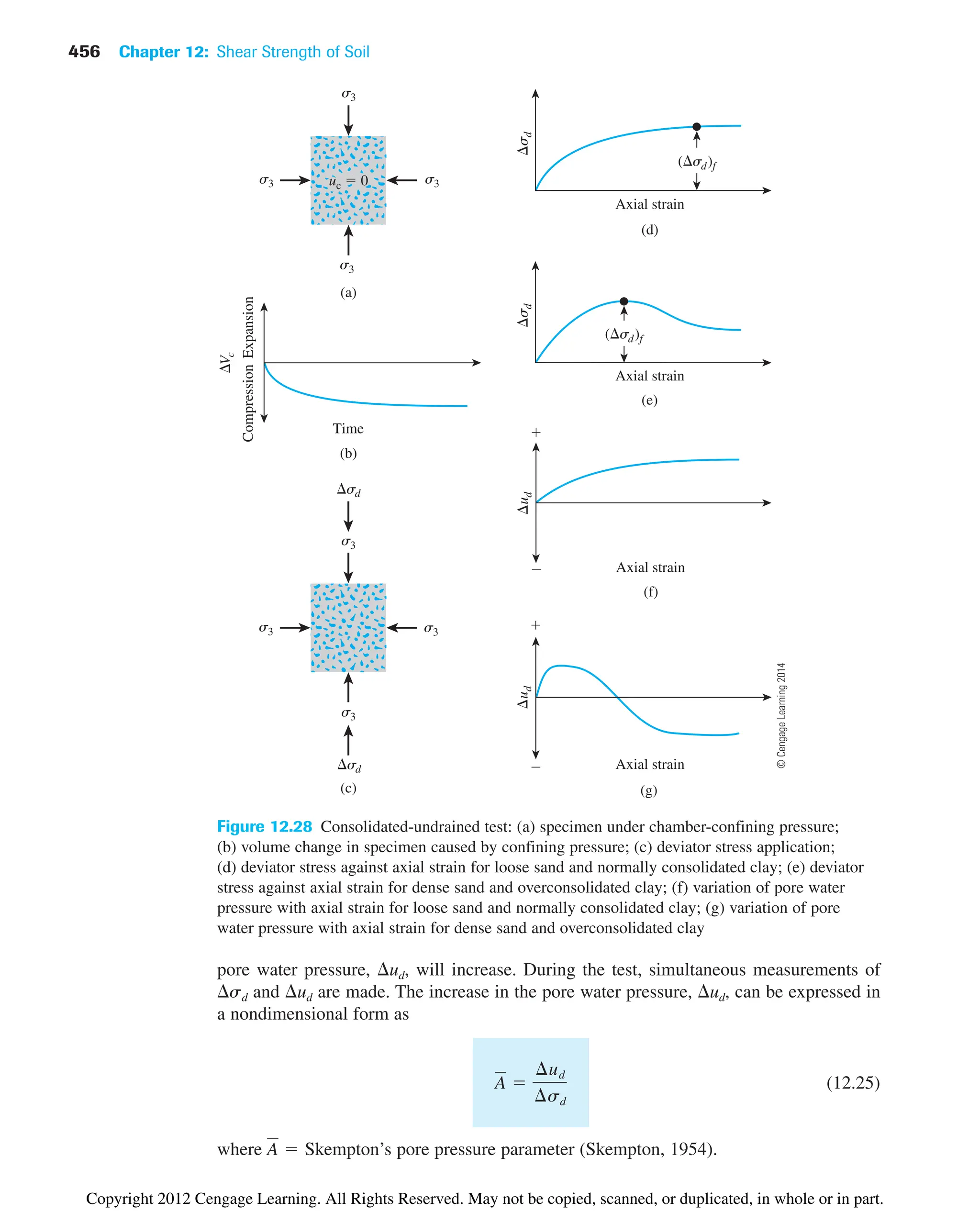
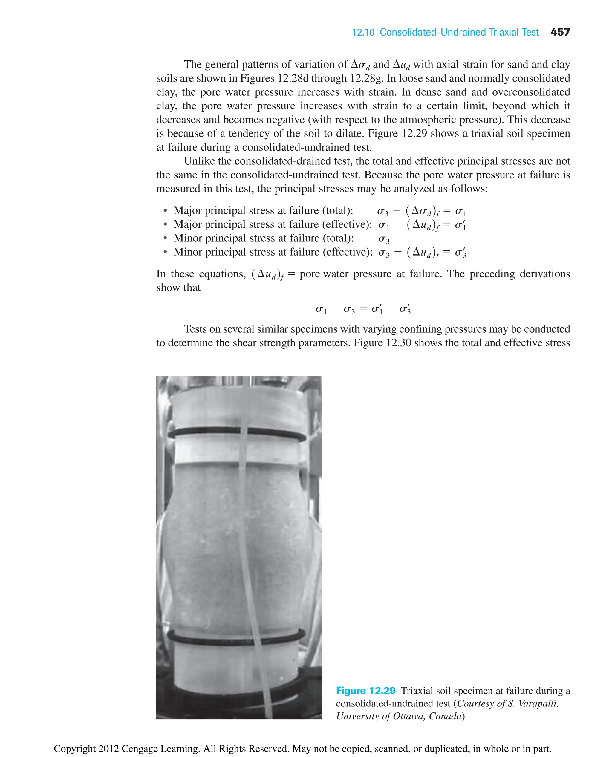
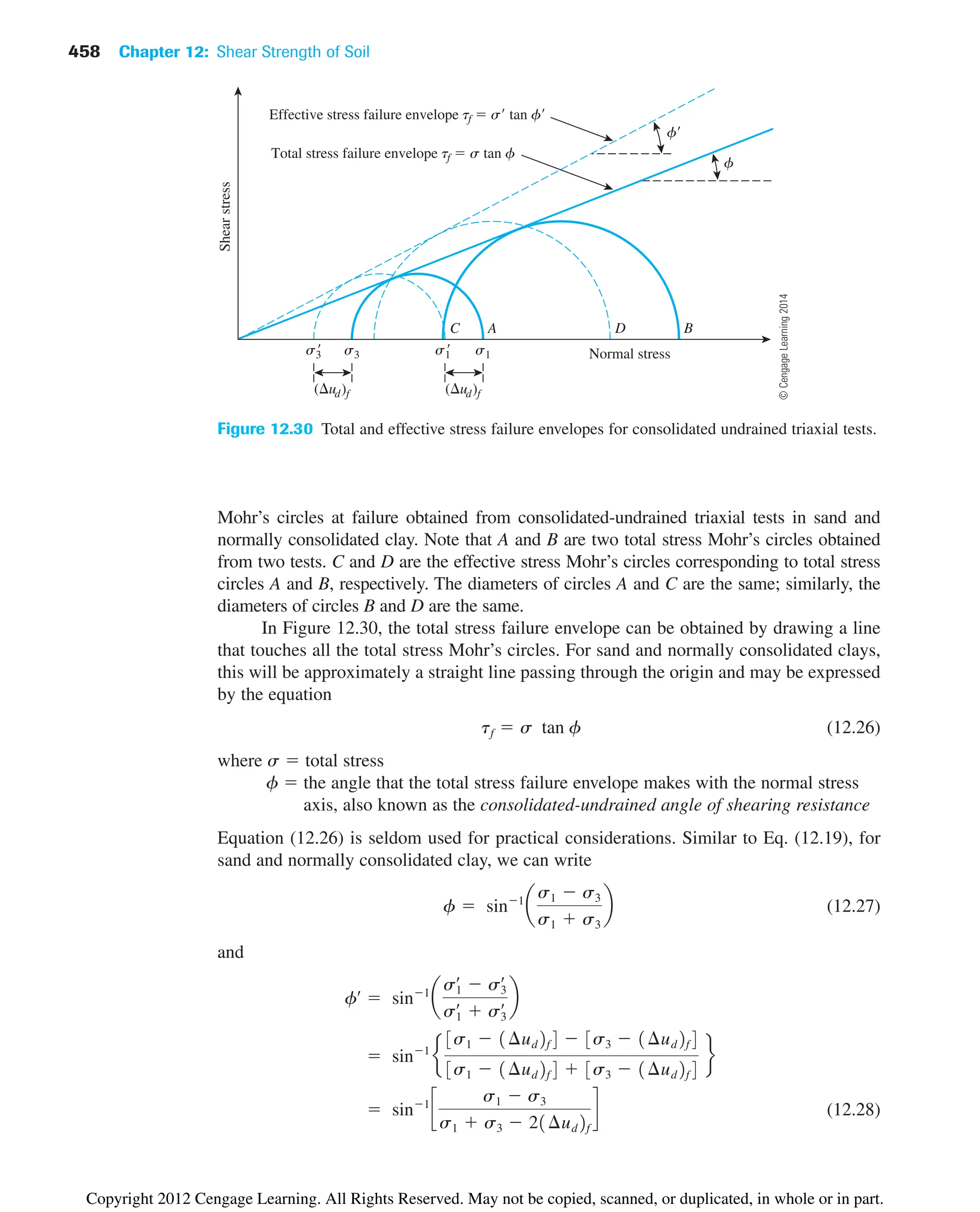
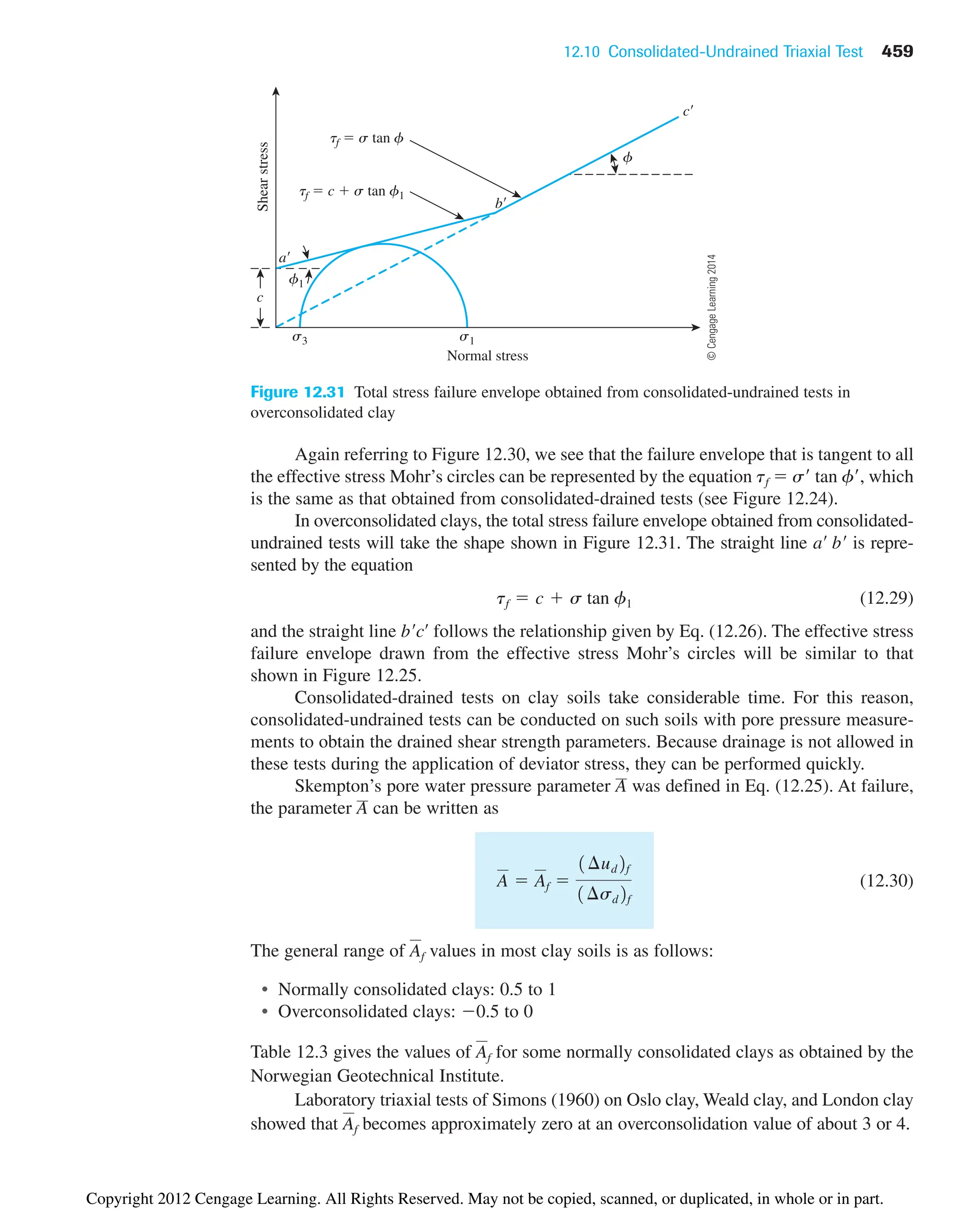
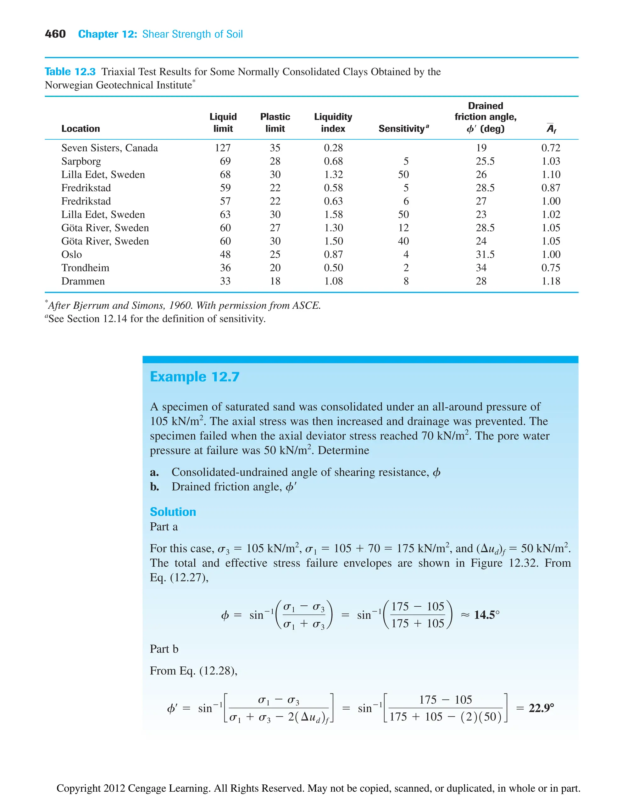
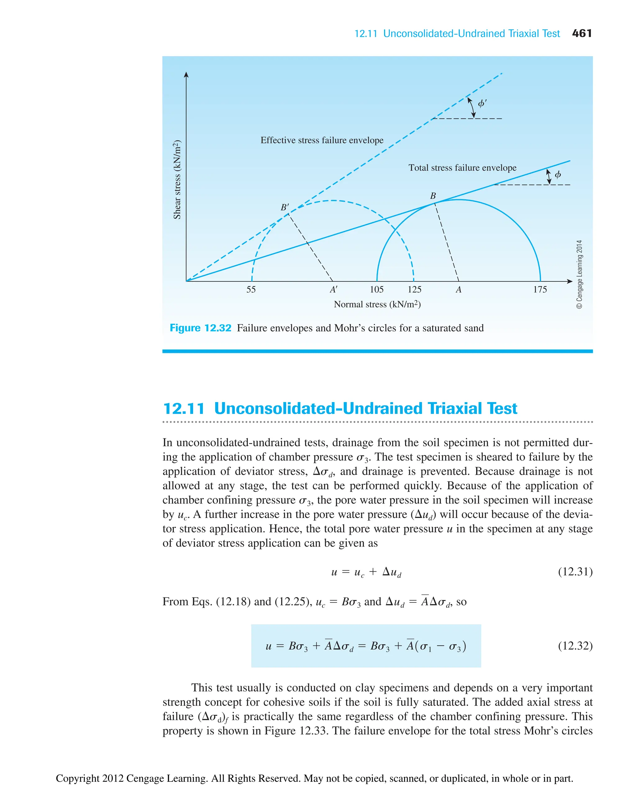
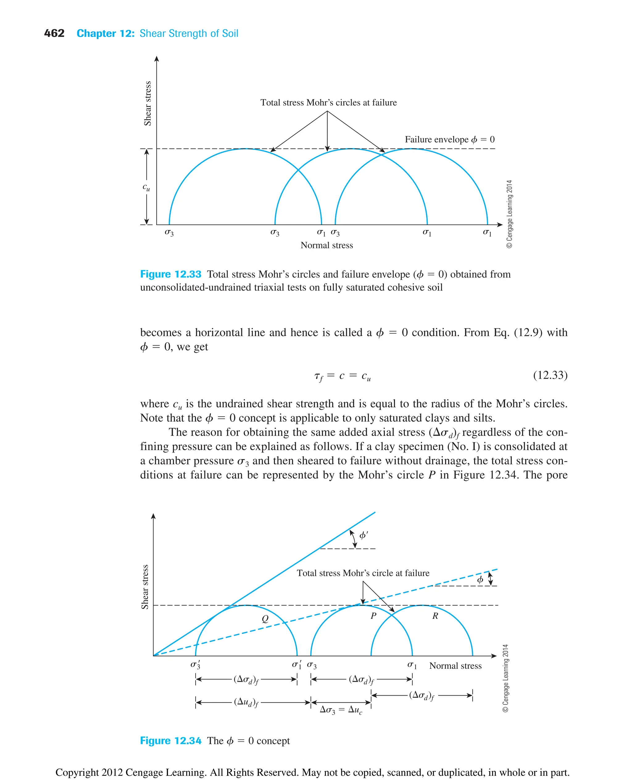
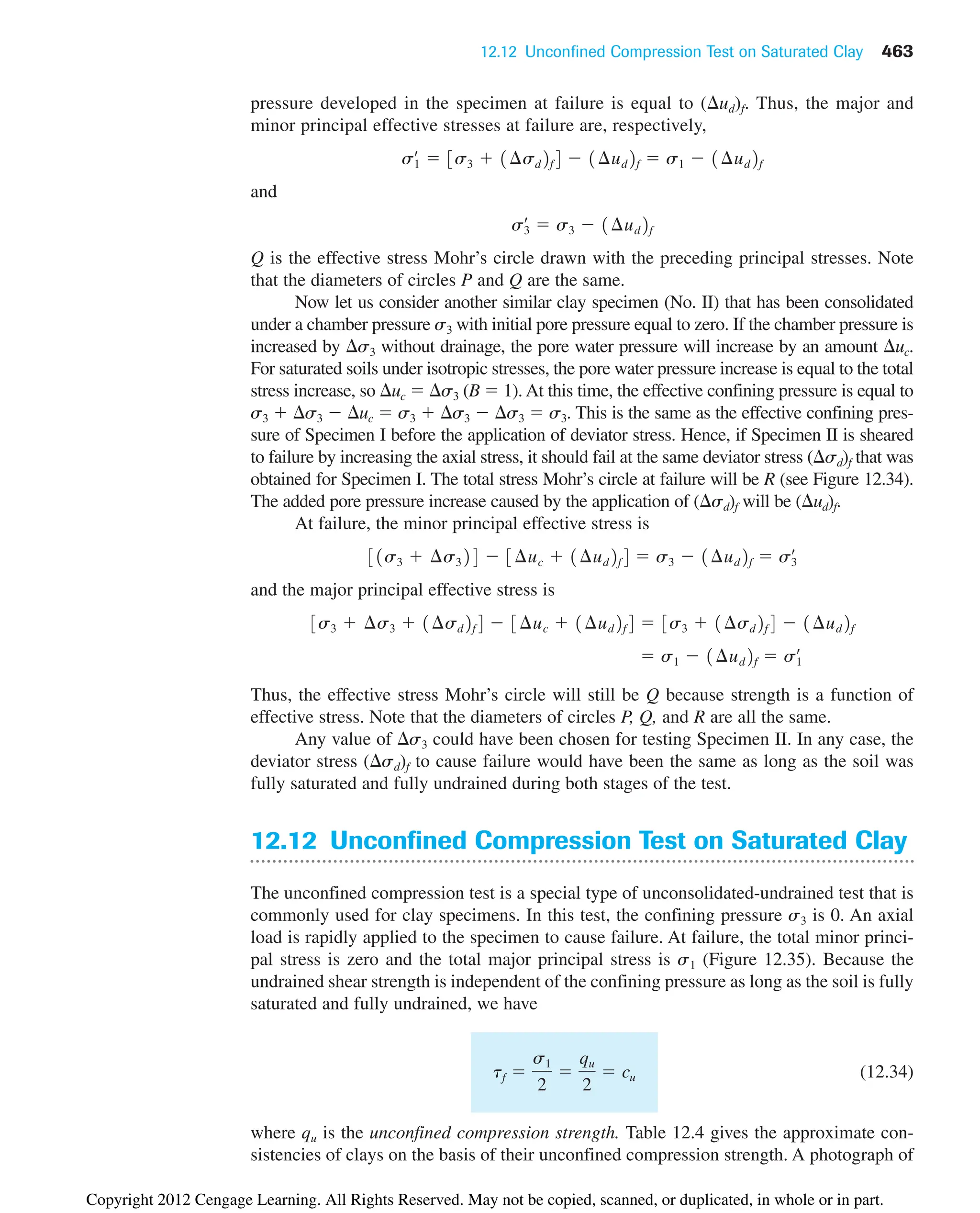
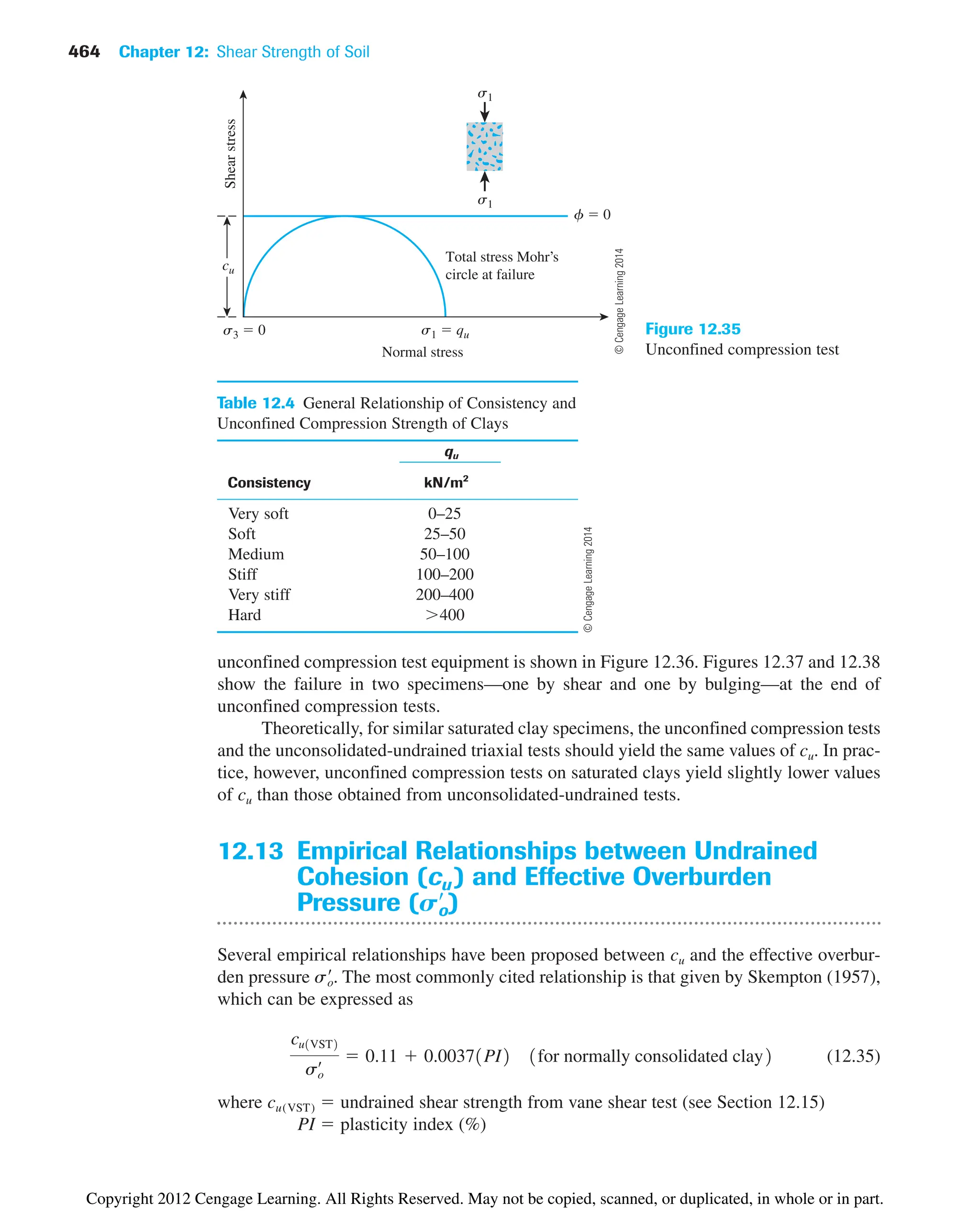

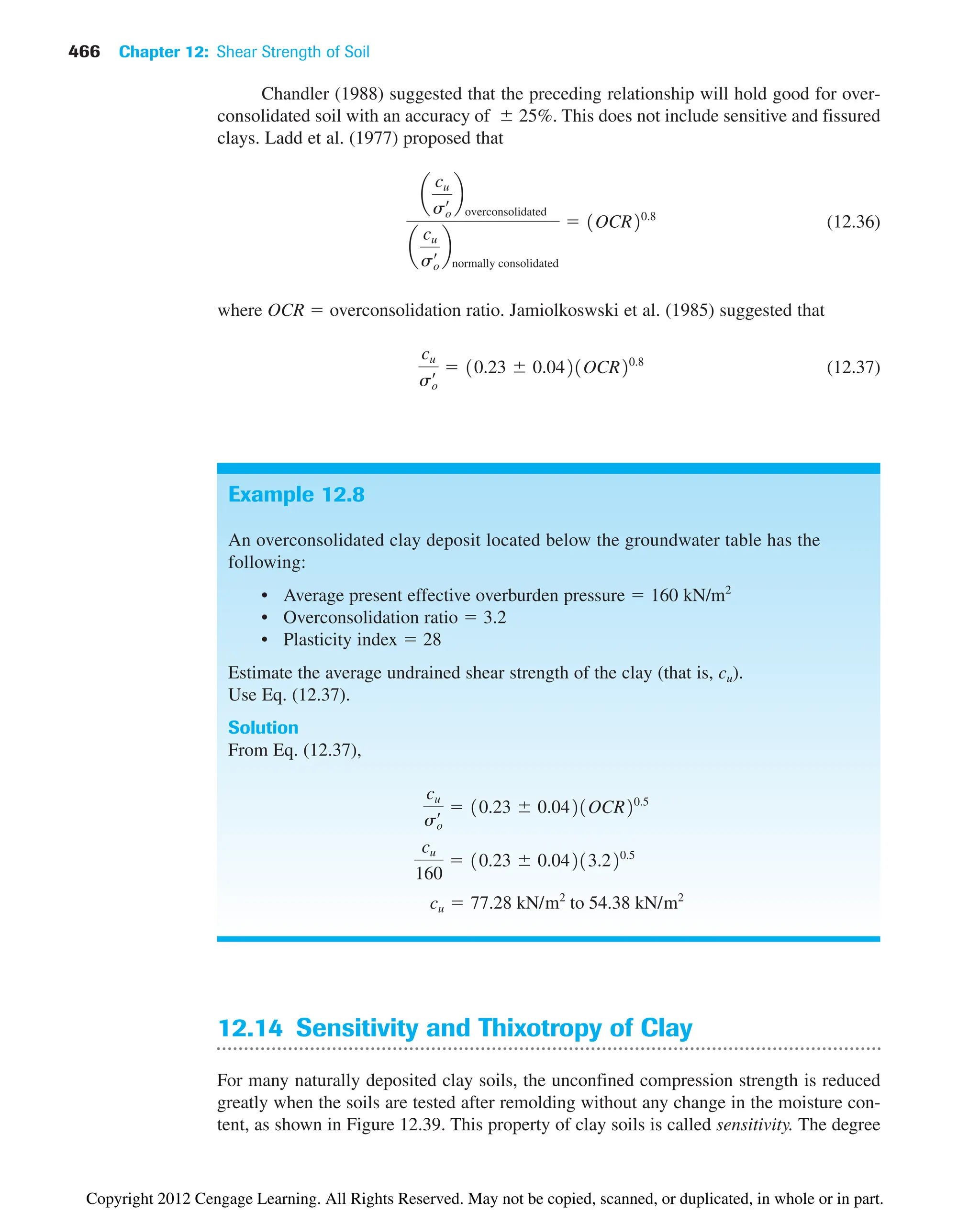
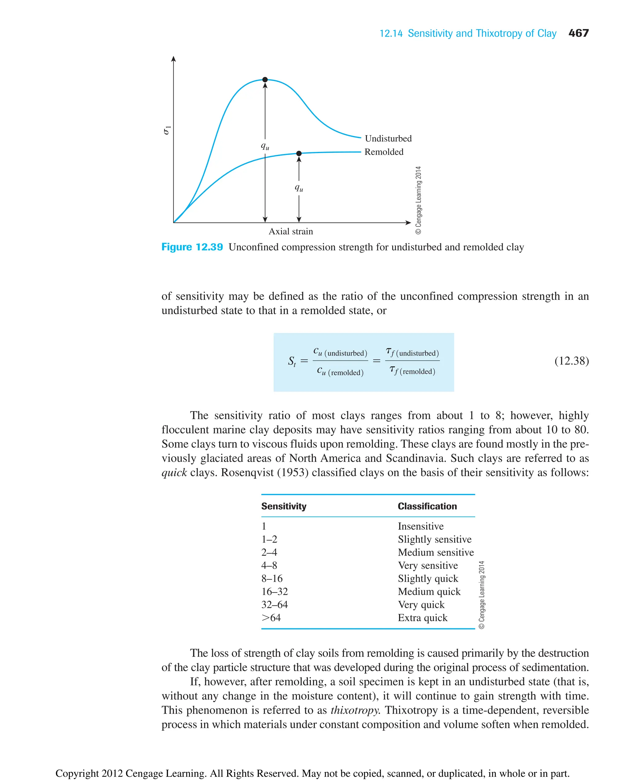
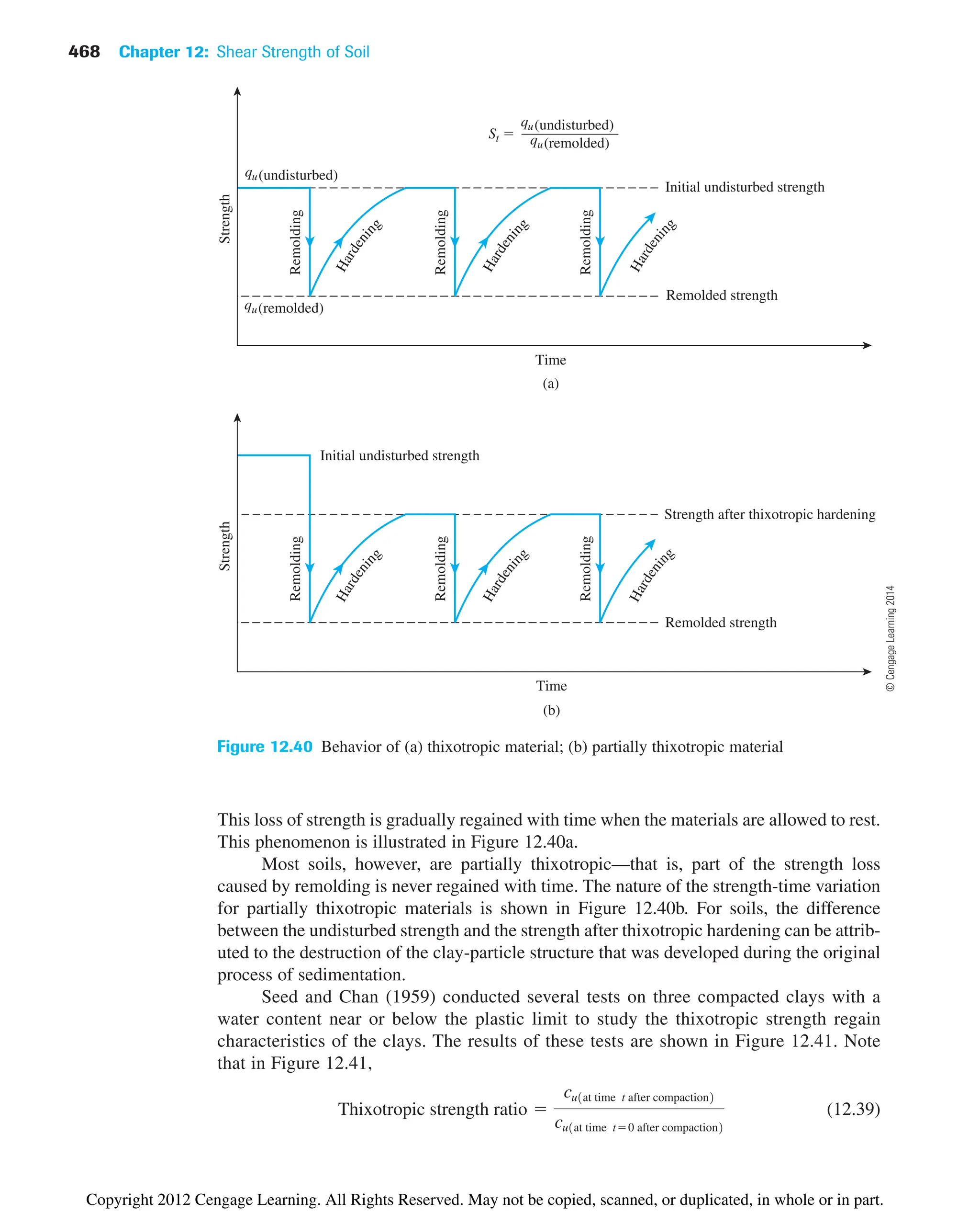
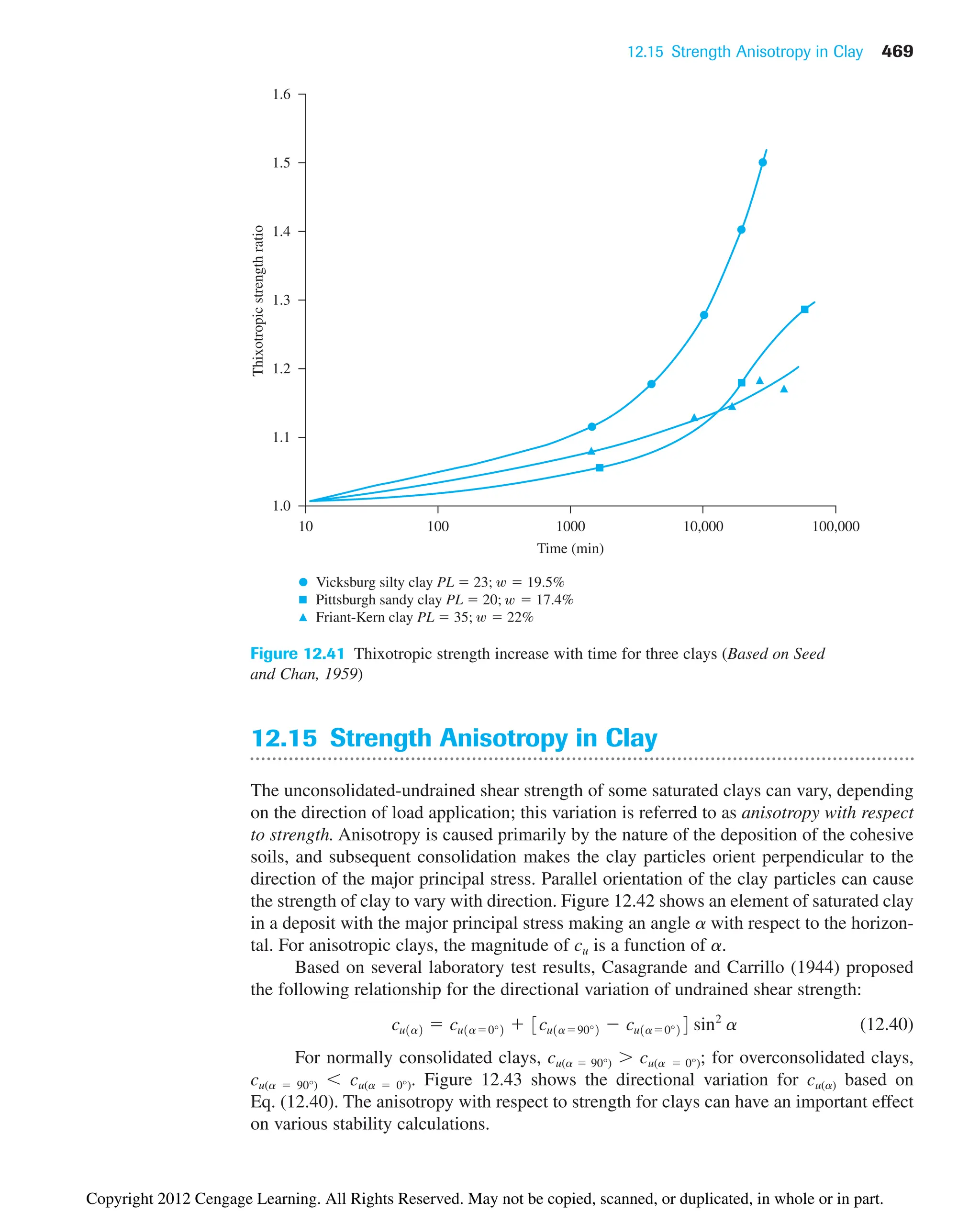
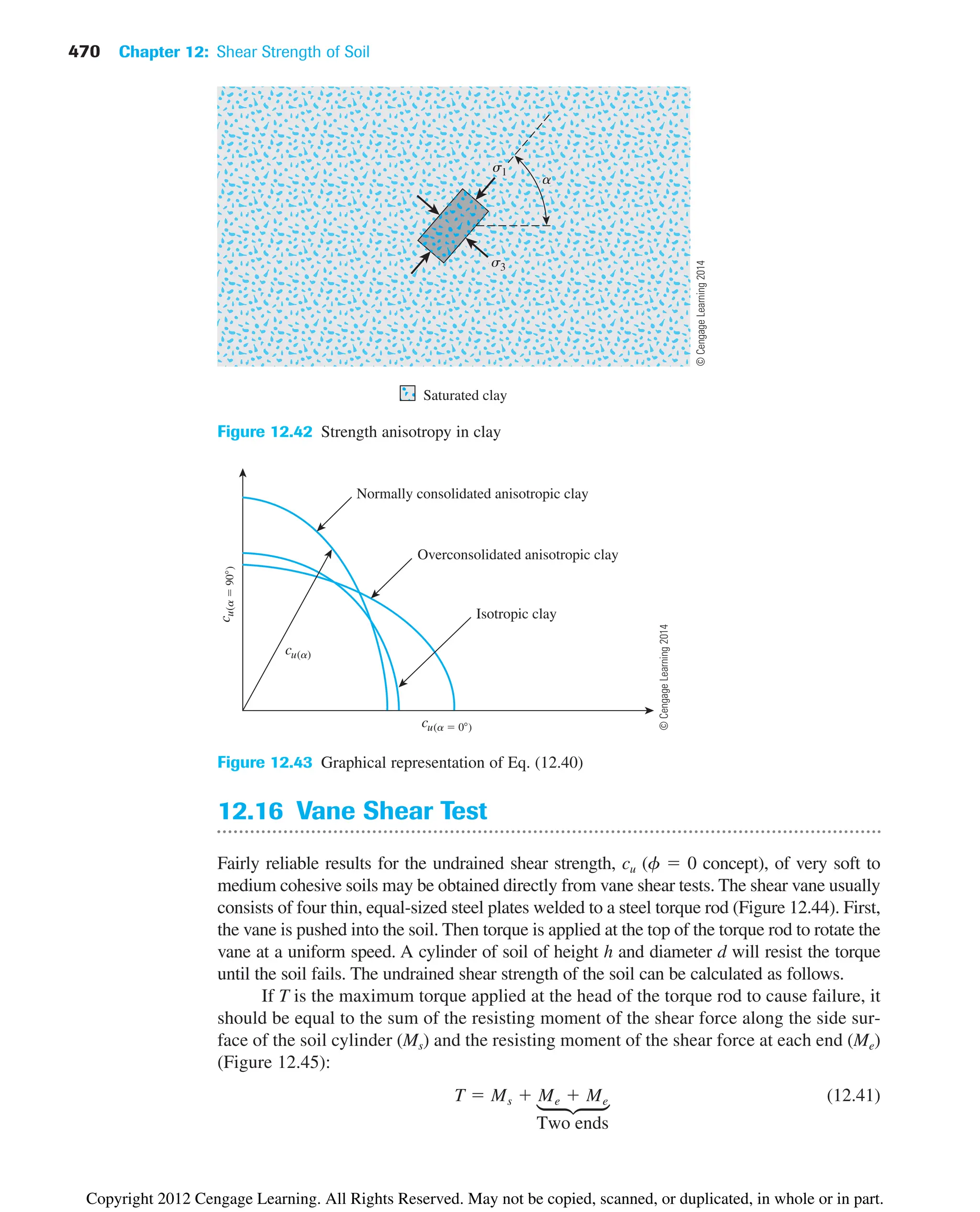
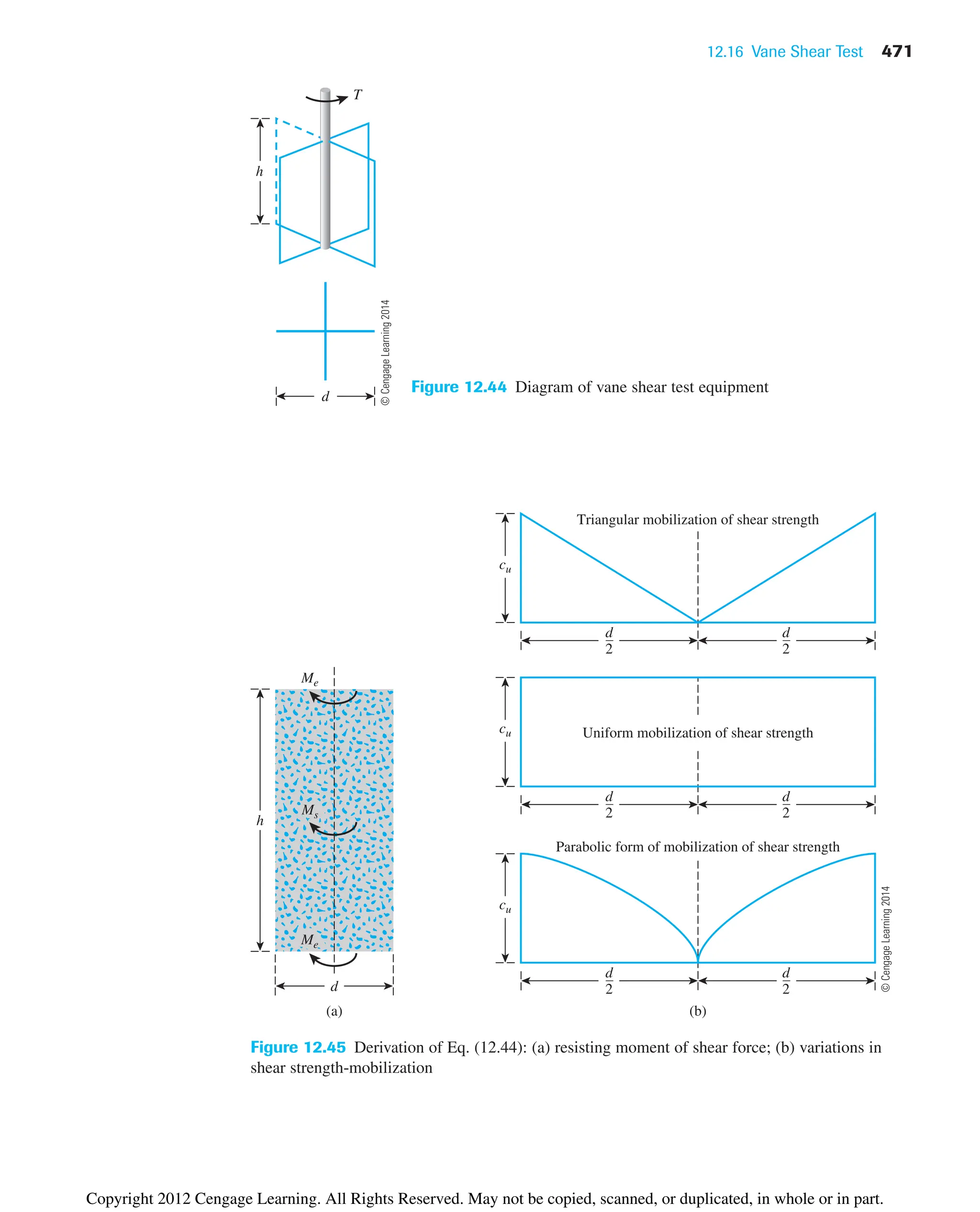
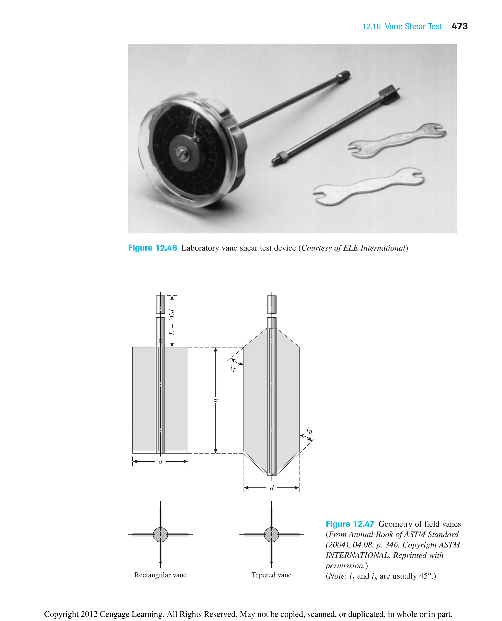
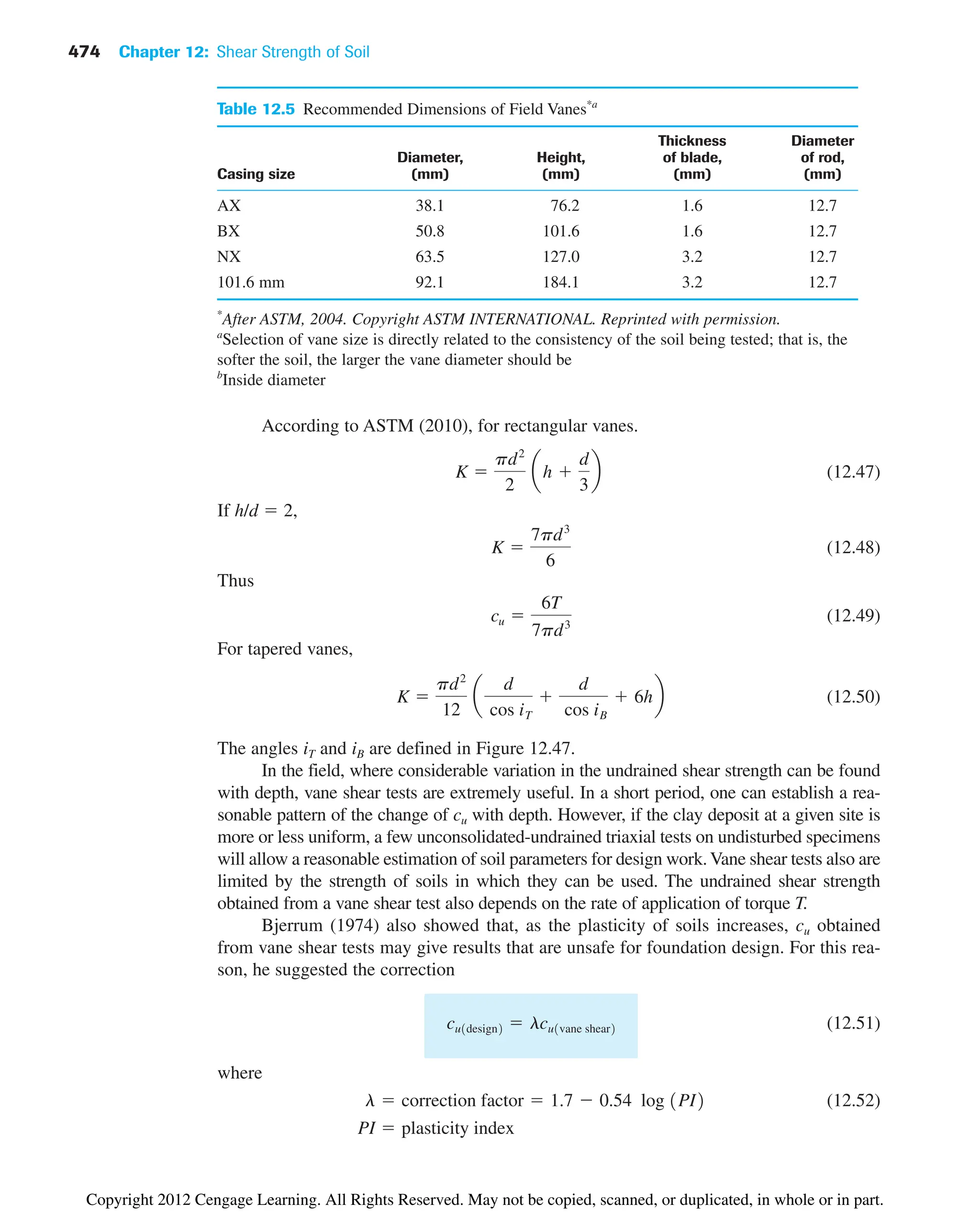
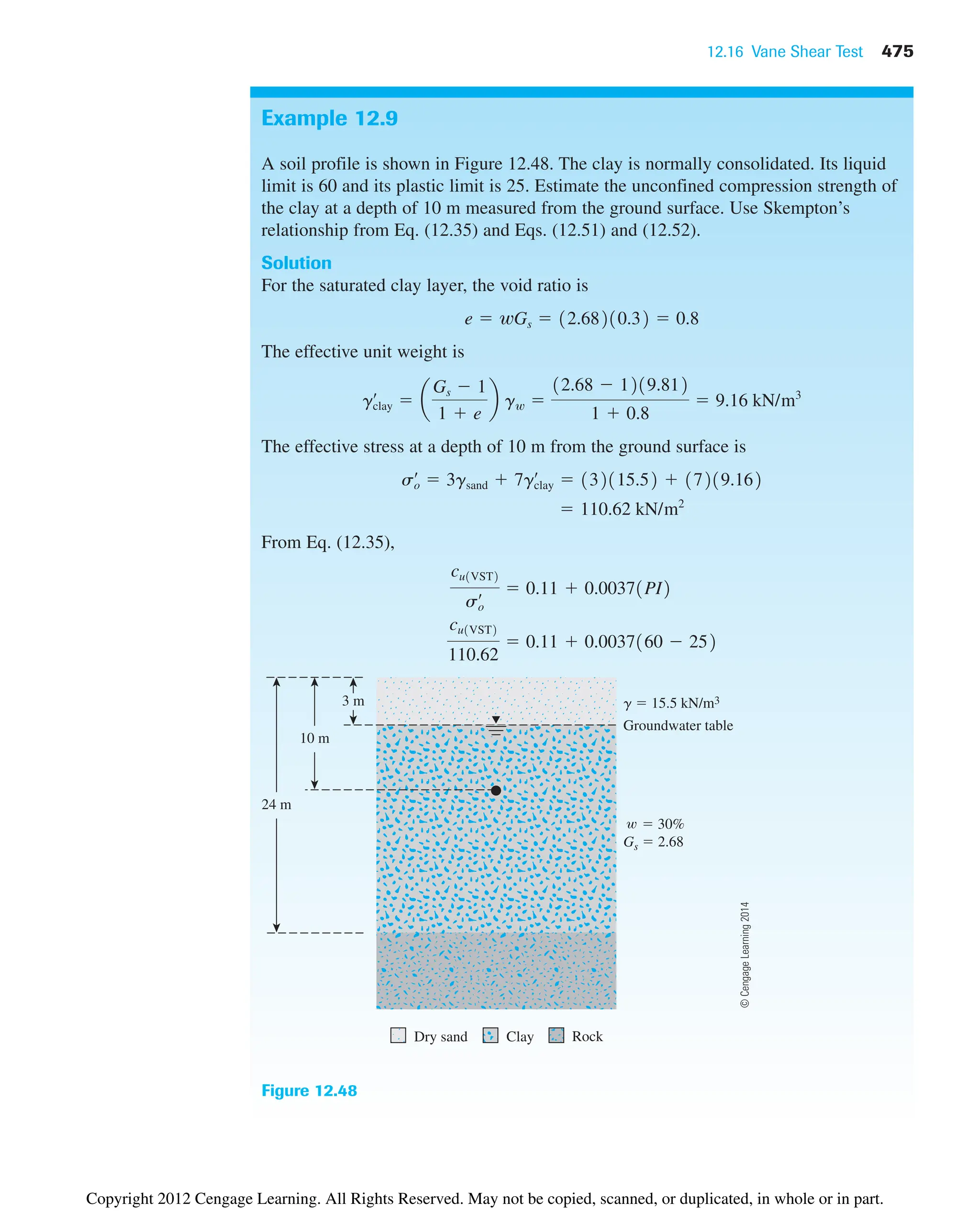
![476 Chapter 12: Shear Strength of Soil
12.17 Other Methods for Determining Undrained
Shear Strength
A modified form of the vane shear test apparatus is the Torvane (Figure 12.49), which is a
handheld device with a calibrated spring. This instrument can be used for determining cu
for tube specimens collected from the field during soil exploration, and it can be used in
the field. The Torvane is pushed into the soil and then rotated until the soil fails. The
undrained shear strength can be read at the top of the calibrated dial.
Figure 12.50 shows a pocket penetrometer, which is pushed directly into the soil. The
unconfined compression strength (qu) is measured by a calibrated spring. This device can
be used both in the laboratory and in the field.
12.18 Shear Strength of Unsaturated Cohesive Soils
The equation relating total stress, effective stress, and pore water pressure for unsaturated
soils can be expressed as
(12.53)
where s effective stress
s total stress
ua pore air pressure
uw pore water pressure
When the expression for s is substituted into the shear strength equation
[Eq. (12.3)], which is based on effective stress parameters, we get
(12.54)
The values of depend primarily on the degree of saturation. With ordinary triaxial
equipment used for laboratory testing, it is not possible to determine accurately the effec-
tive stresses in unsaturated soil specimens, so the common practice is to conduct undrained
tf cœ
3s ua x1ua uw24 tan fœ
sœ
s ua x1ua uw2
and
From Eqs. (12.51) and (12.52), we get
So the unconfined compression strength is
qu 2cu 122122.952 45.9 kN/m2
31.7 0.54 log 160 252426.49 22.95 kN/m2
31.7 0.54 log 1PI24cu1VST2
cu lcu1VST2
cu1VST2 26.49 kN/m2
Copyright 2012 Cengage Learning. All Rights Reserved. May not be copied, scanned, or duplicated, in whole or in part.](https://image.slidesharecdn.com/principlesofgeotechnicalengineering-8thedition-231222125509-7e44d9bf/75/Principles-of-Geotechnical-Engineering-8th-Edition-pdf-496-2048.jpg)

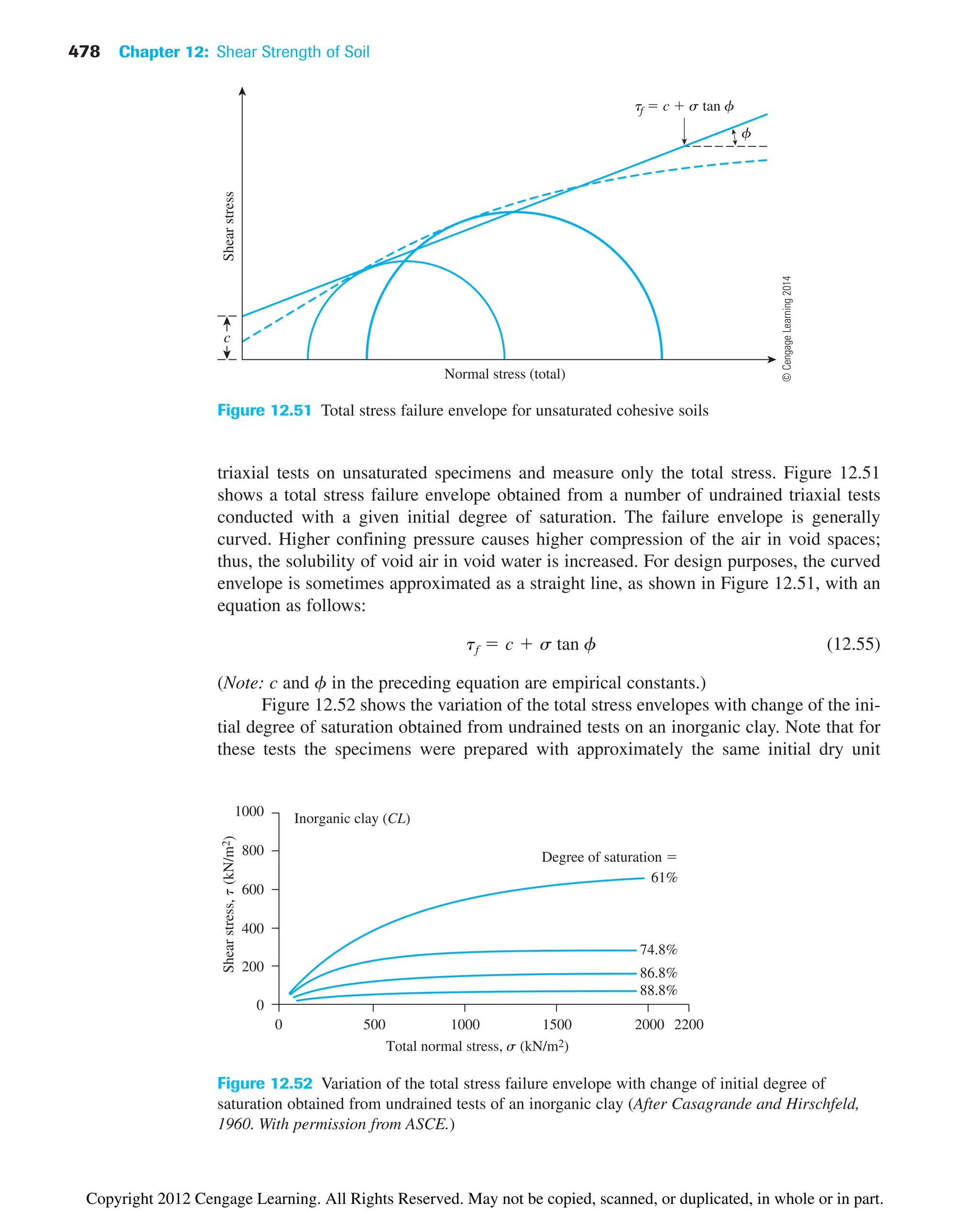
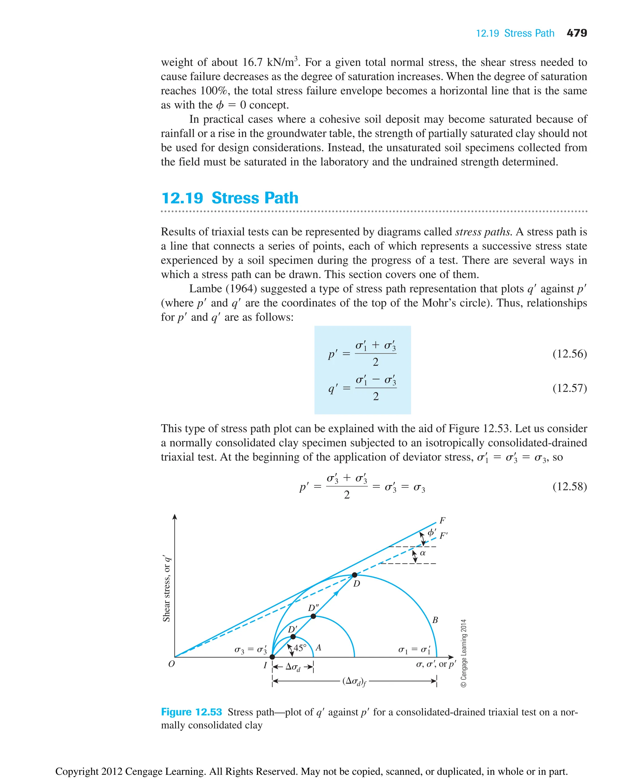
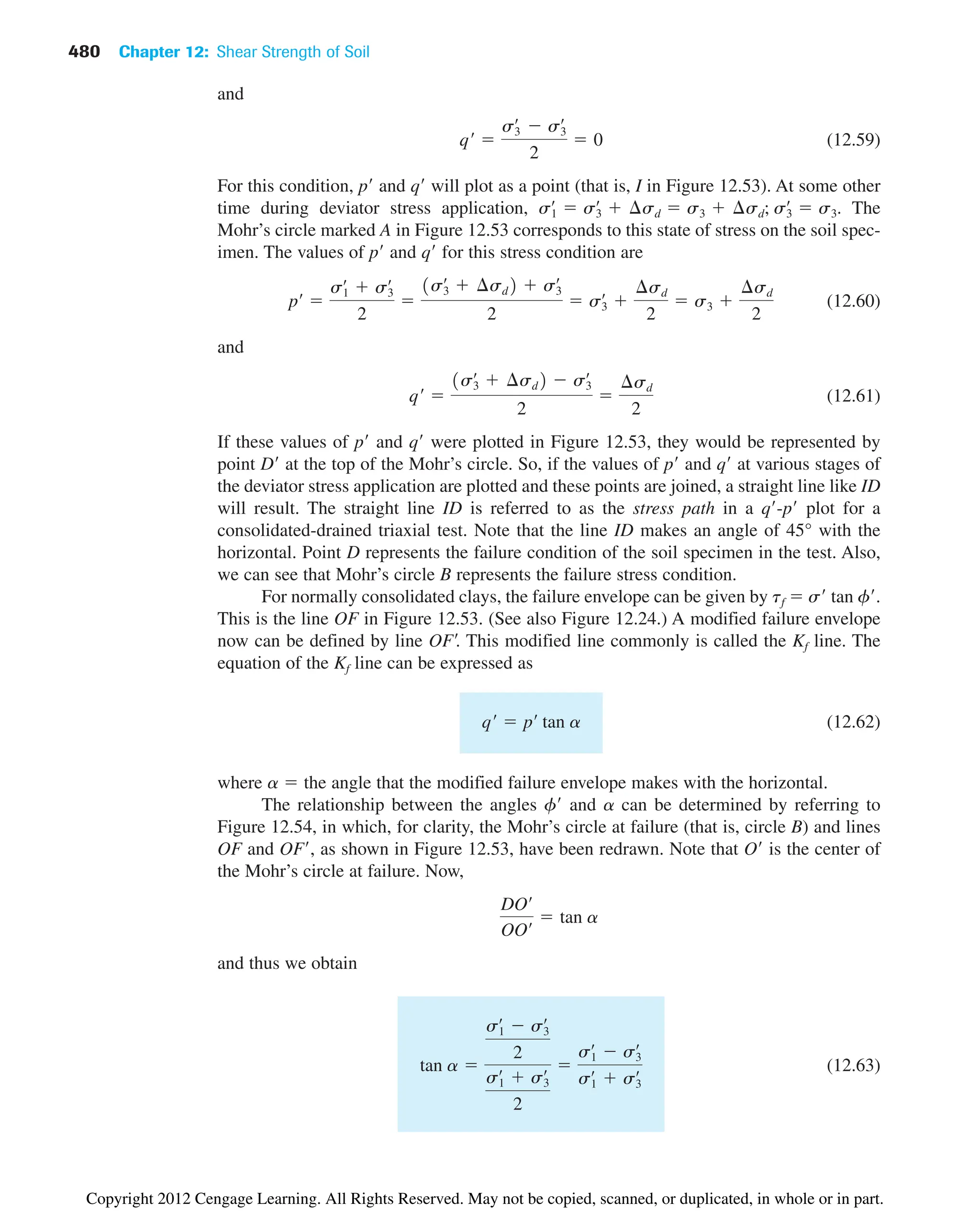
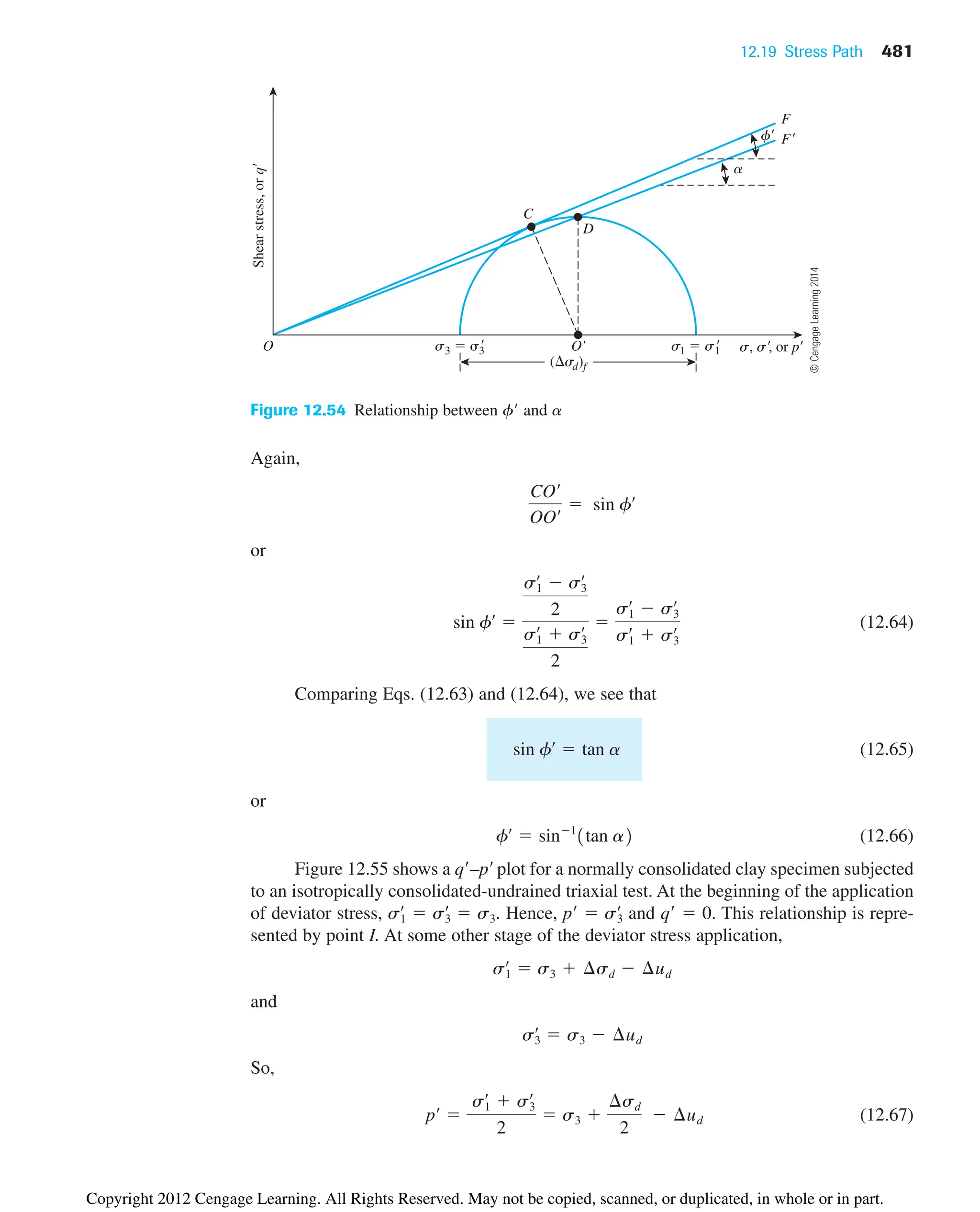
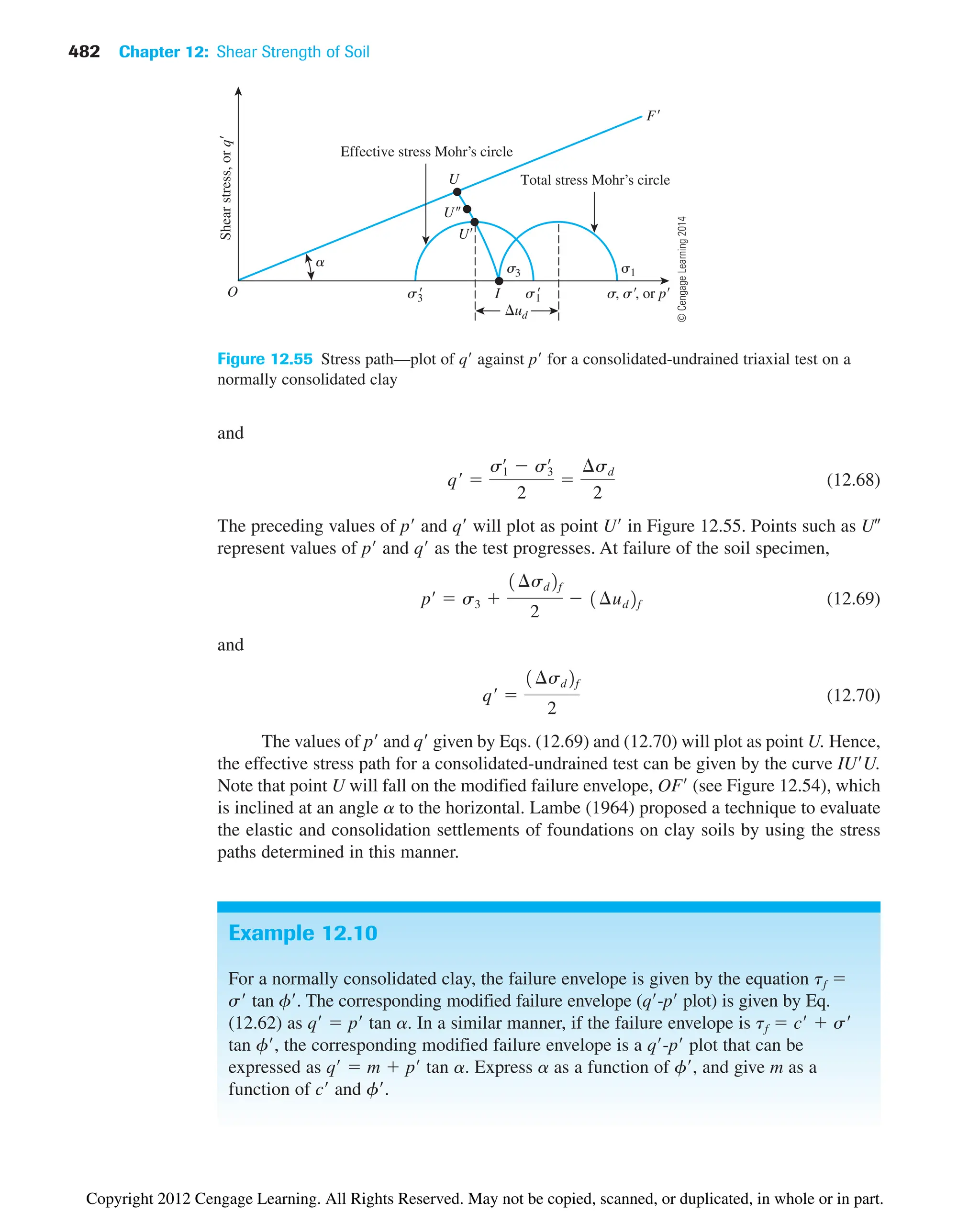
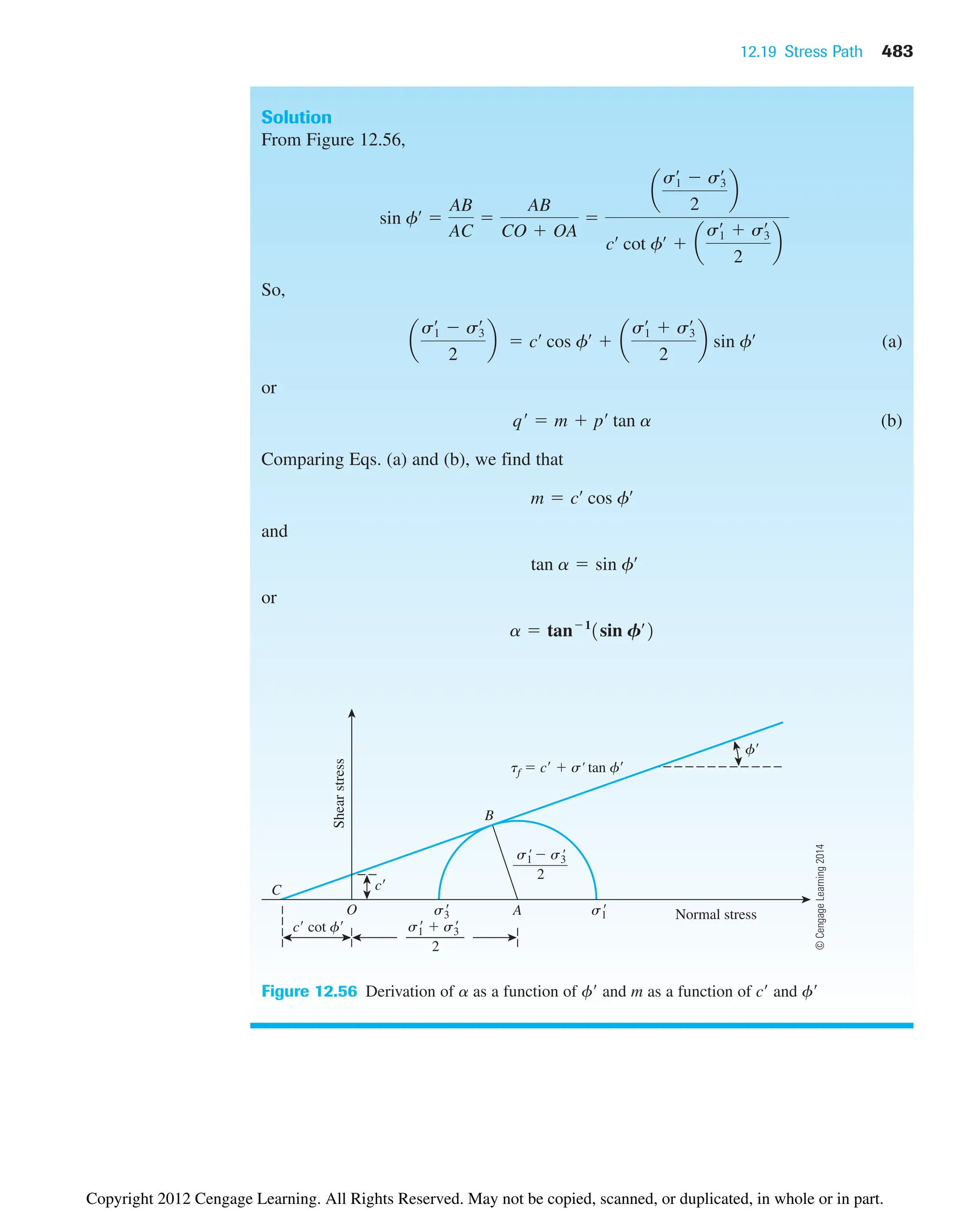
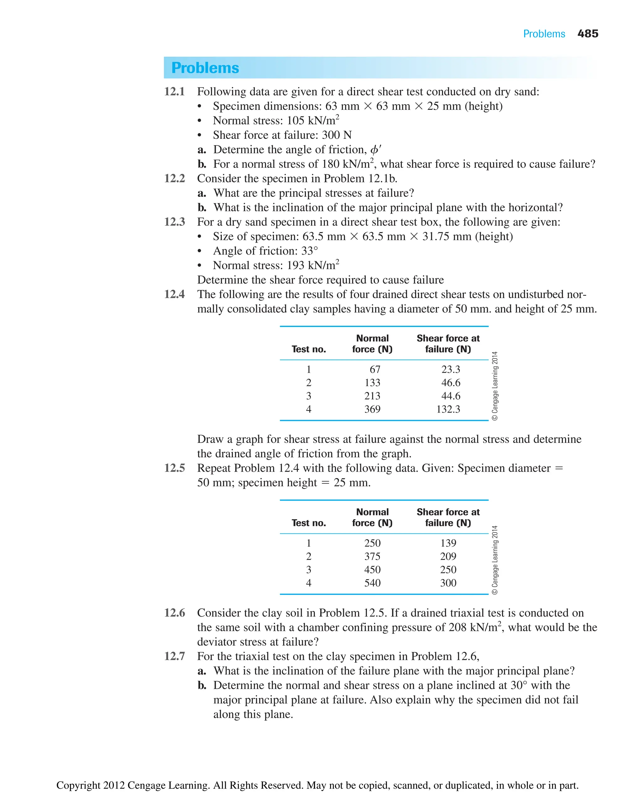
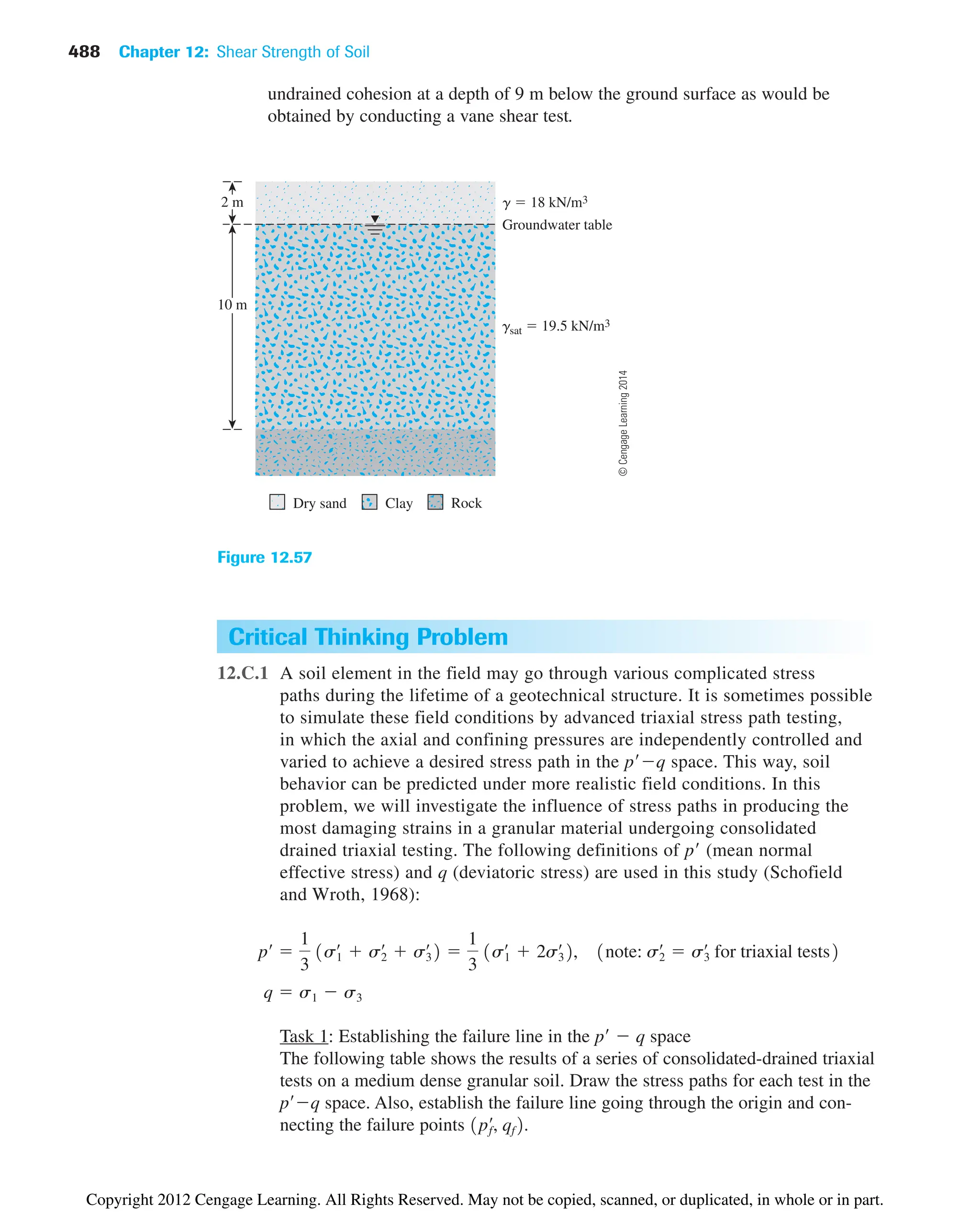
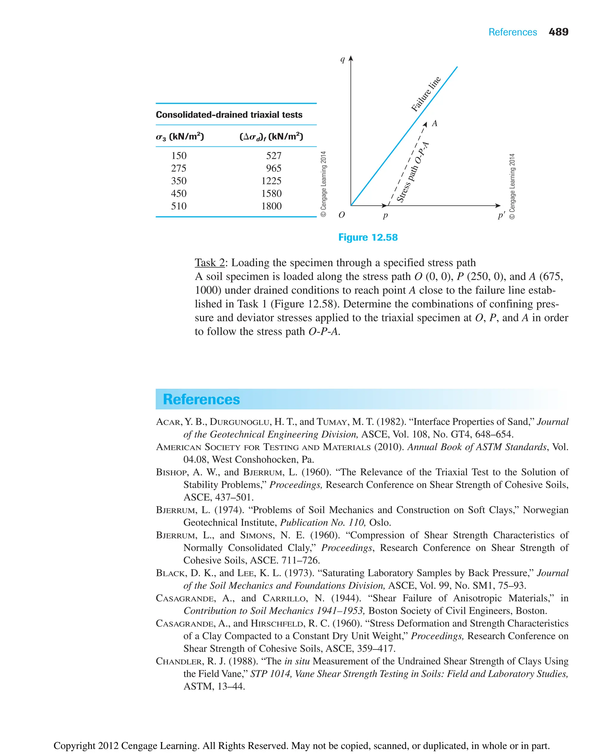
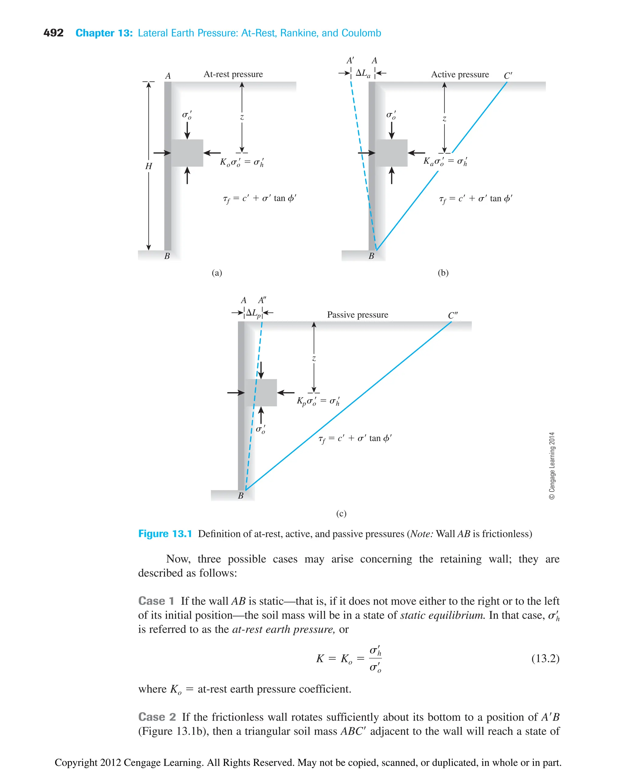
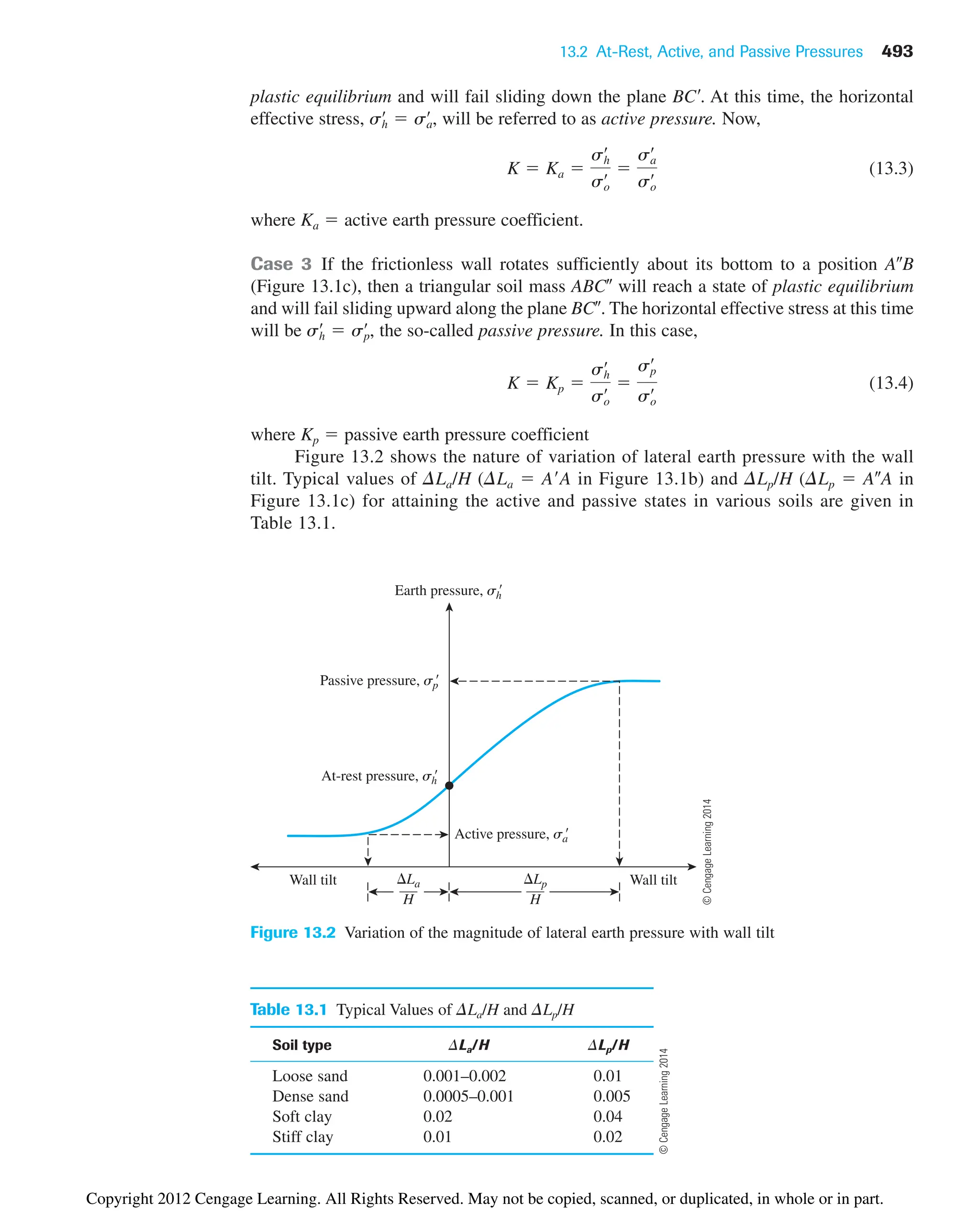
![494 Chapter 13: Lateral Earth Pressure: At-Rest, Rankine, and Coulomb
A
B
so
gz
sh
Kogz
H
z
tf c s tan f
Figure 13.3
Earth pressure at rest
AT-REST LATERAL EARTH PRESSURE
13.3 Earth Pressure At-Rest
The fundamental concept of earth pressure at rest was discussed in the preceding section. In
order to define the earth pressure coefficient Ko at rest, we refer to Figure 13.3, which shows
a wall AB retaining a dry soil with a unit weight of g. The wall is static. At a depth z,
So,
For coarse-grained soils, the coefficient of earth pressure at rest can be estimated by
using the empirical relationship (Jaky, 1944)
(13.5)
where f drained friction angle.
While designing a wall that may be subjected to lateral earth pressure at rest, one
must take care in evaluating the value of Ko. Sherif, Fang, and Sherif (1984), on the basis
of their laboratory tests, showed that Jaky’s equation for Ko [Eq. (13.5)] gives good results
when the backfill is loose sand. However, for a dense, compacted sand backfill, Eq. (13.5)
may grossly underestimate the lateral earth pressure at rest. This underestimation results
because of the process of compaction of backfill. For this reason, they recommended the
design relationship
(13.6)
where gd actual compacted dry unit weight of the sand behind the wall
gd(min) dry unit weight of the sand in the loosest state (Chapter 3)
Ko 11 sin f2 c
gd
gd1min2
1d5.5
Ko 1 sin fœ
Ko
sh
œ
so
œ at-rest earth pressure coefficient
Horizontal effective stress sh
œ
Ko gz
Vertical effective stress so
œ
gz
©
Cengage
Learning
2014
Copyright 2012 Cengage Learning. All Rights Reserved. May not be copied, scanned, or duplicated, in whole or in part.](https://image.slidesharecdn.com/principlesofgeotechnicalengineering-8thedition-231222125509-7e44d9bf/75/Principles-of-Geotechnical-Engineering-8th-Edition-pdf-514-2048.jpg)
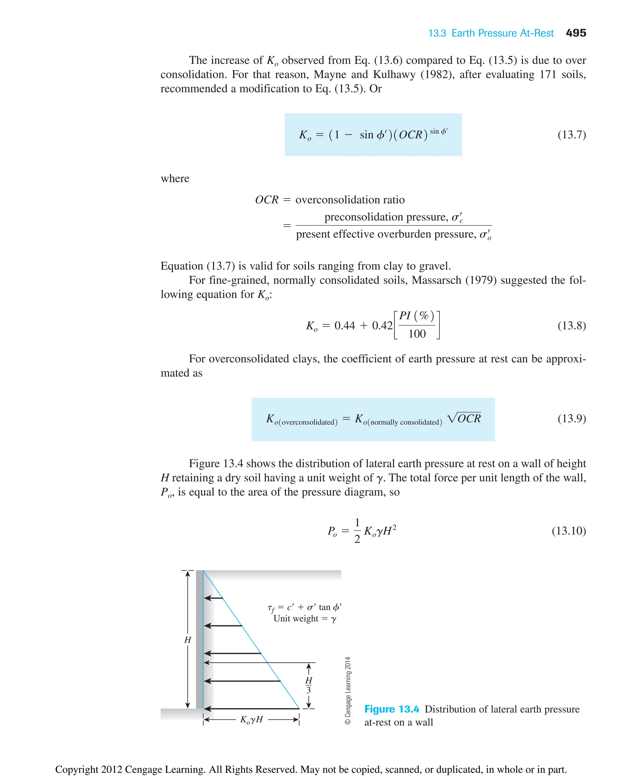
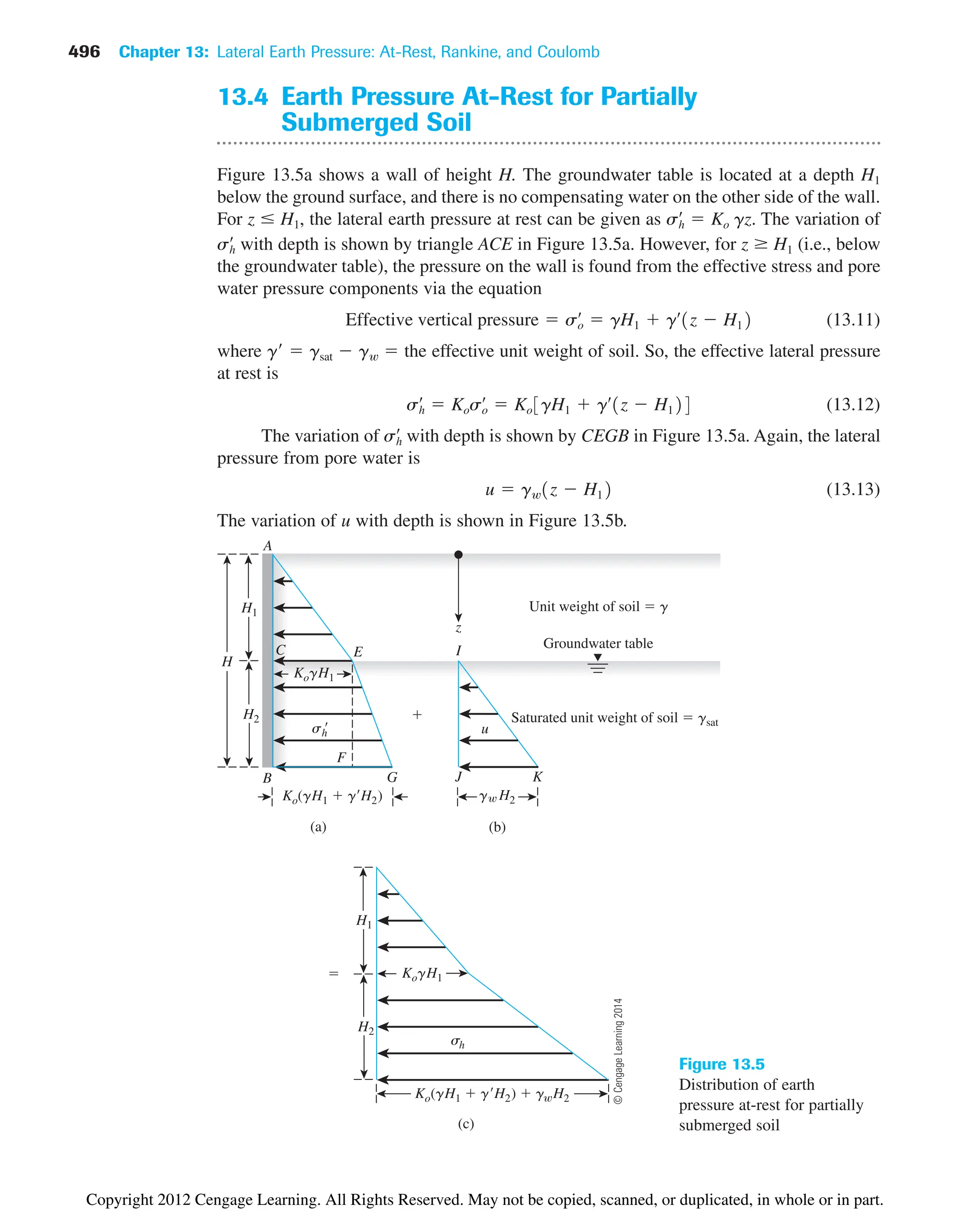
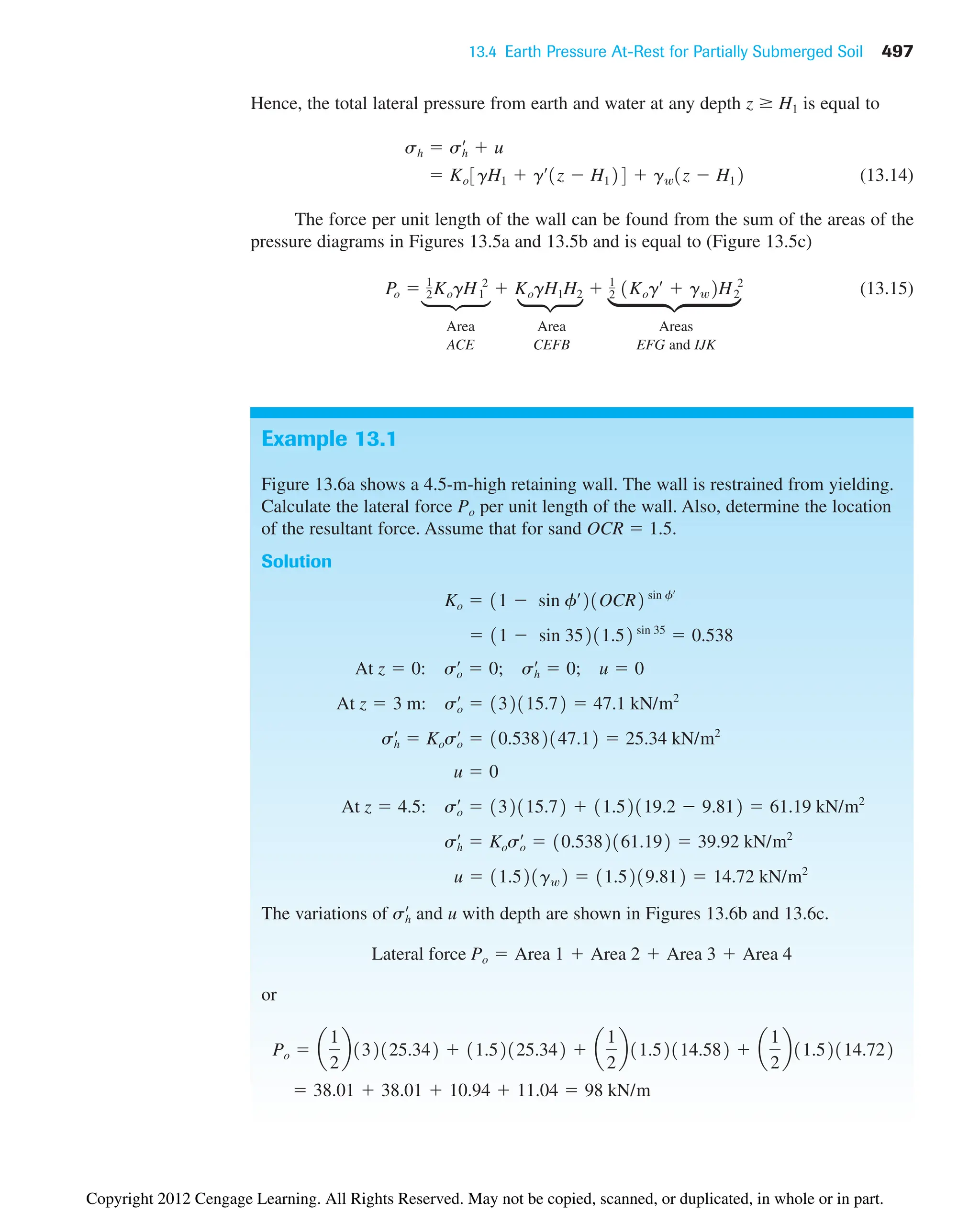
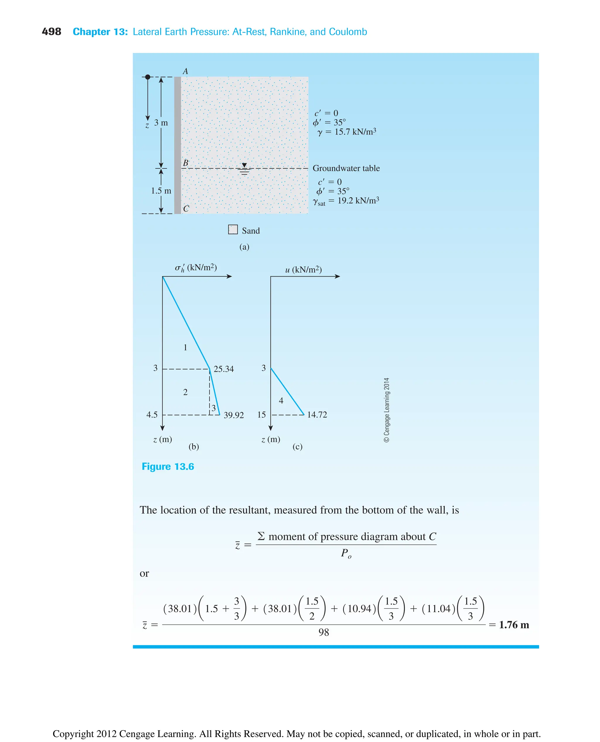
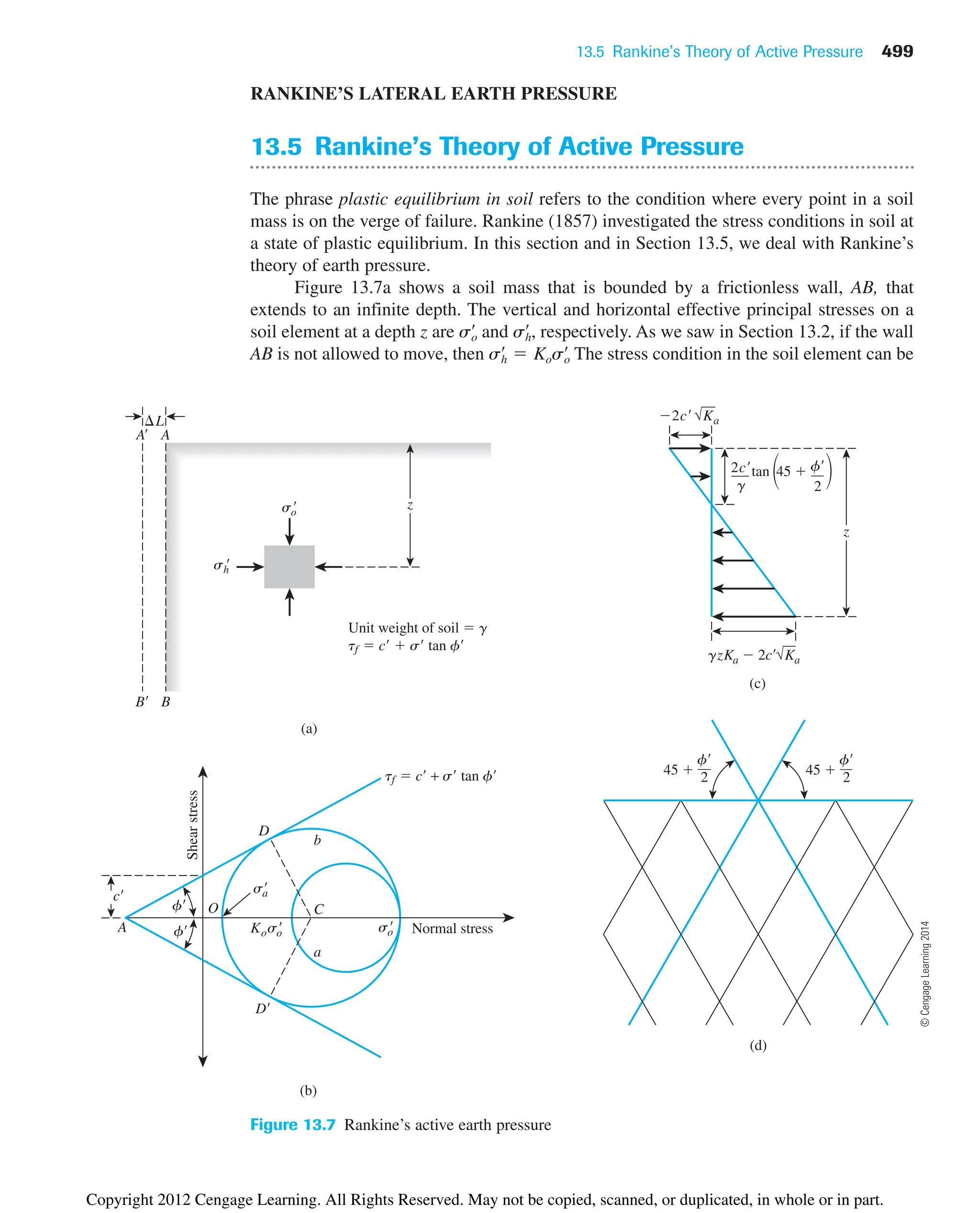
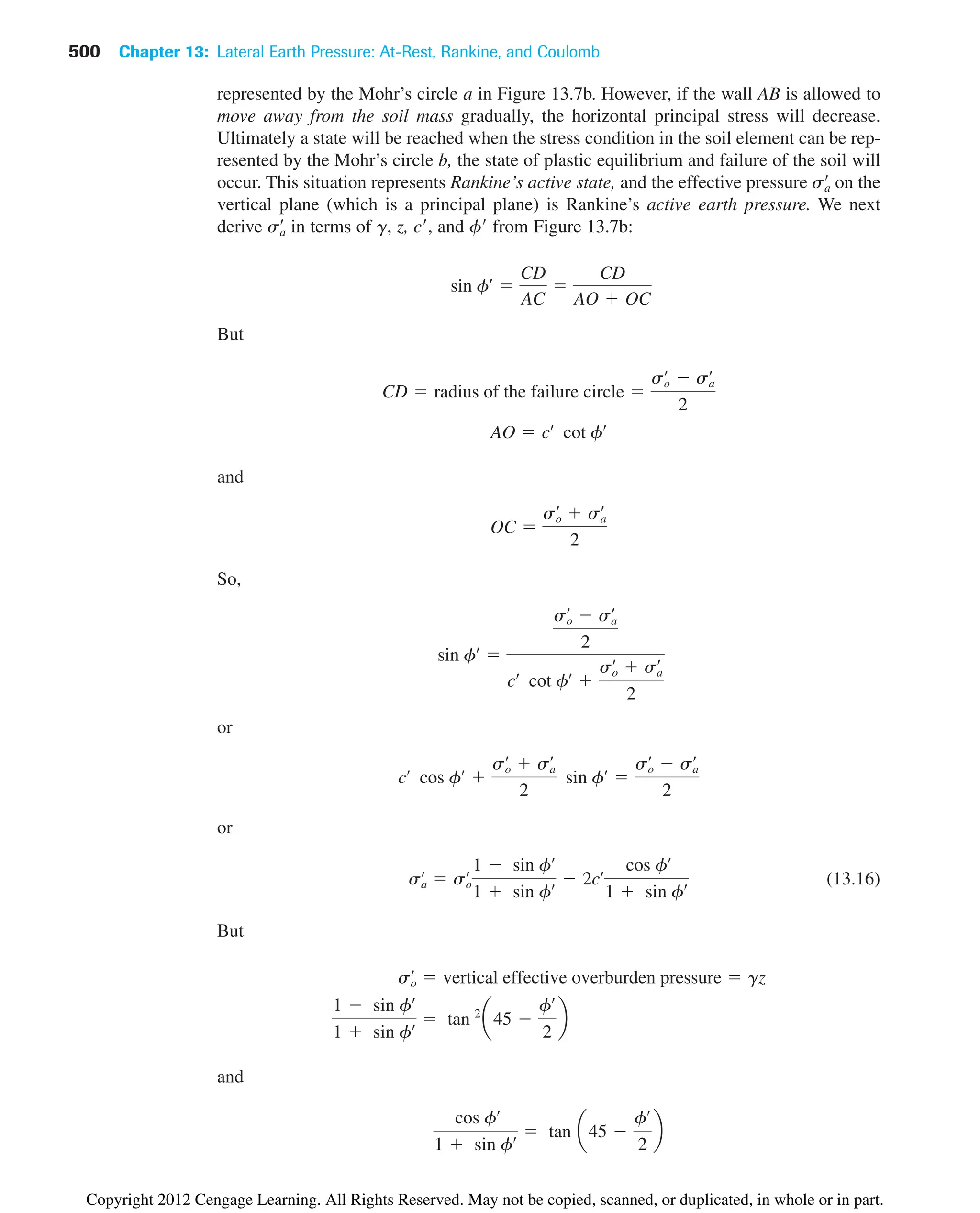
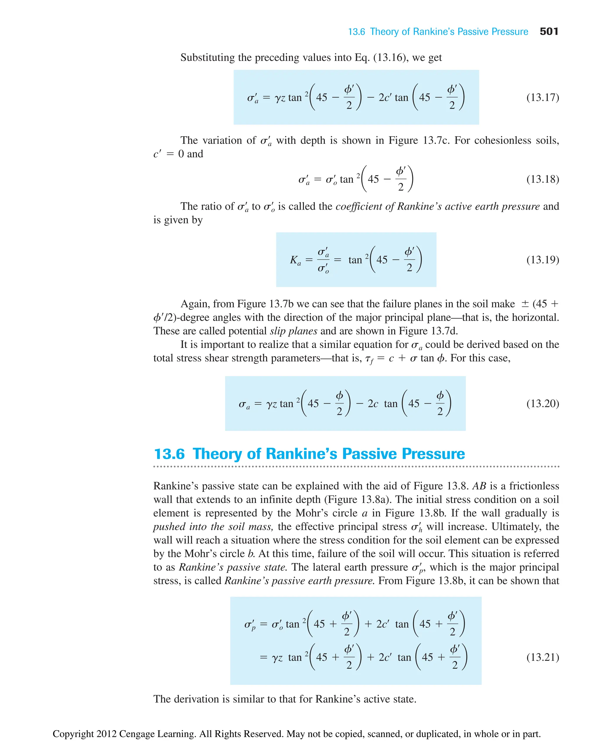
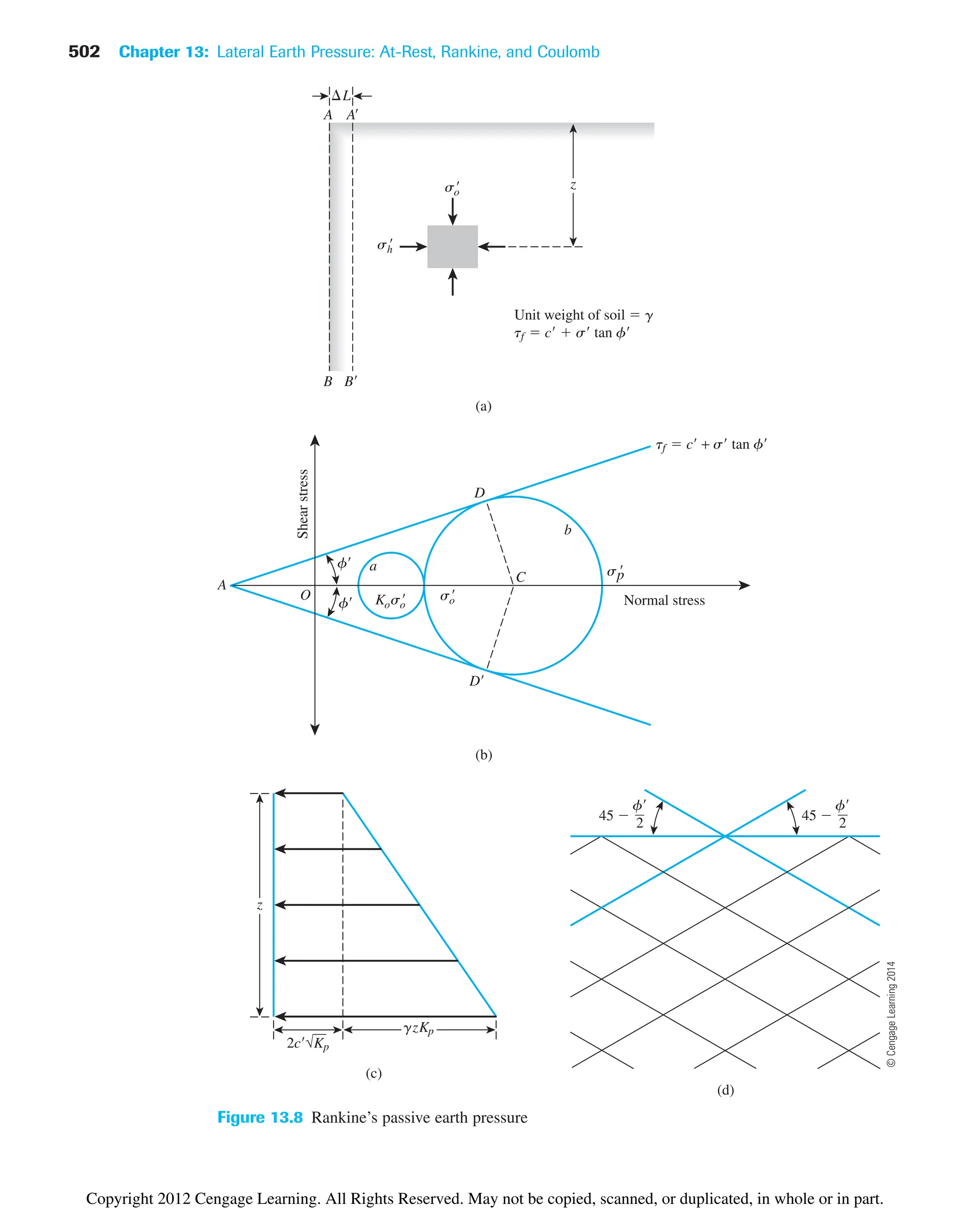
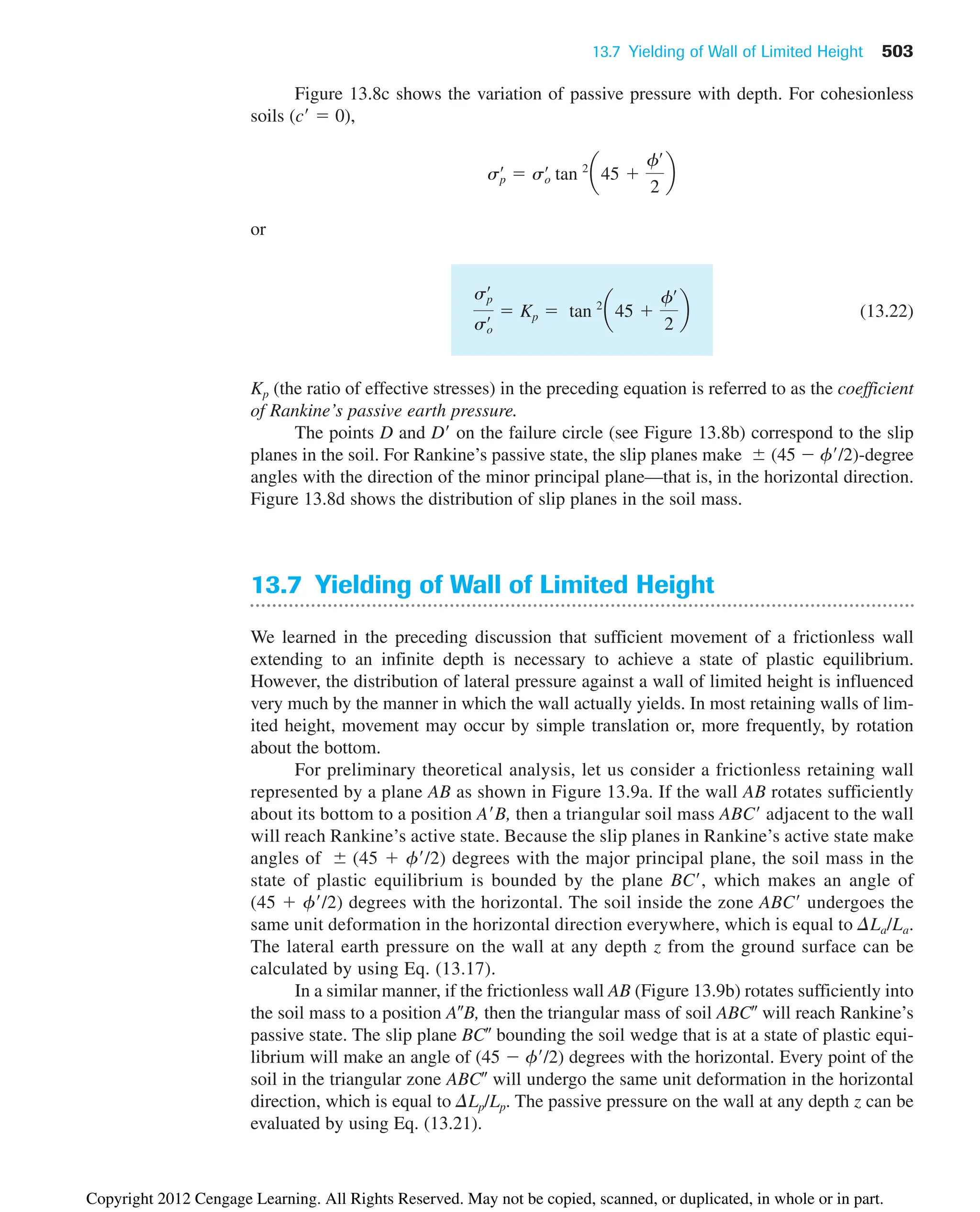
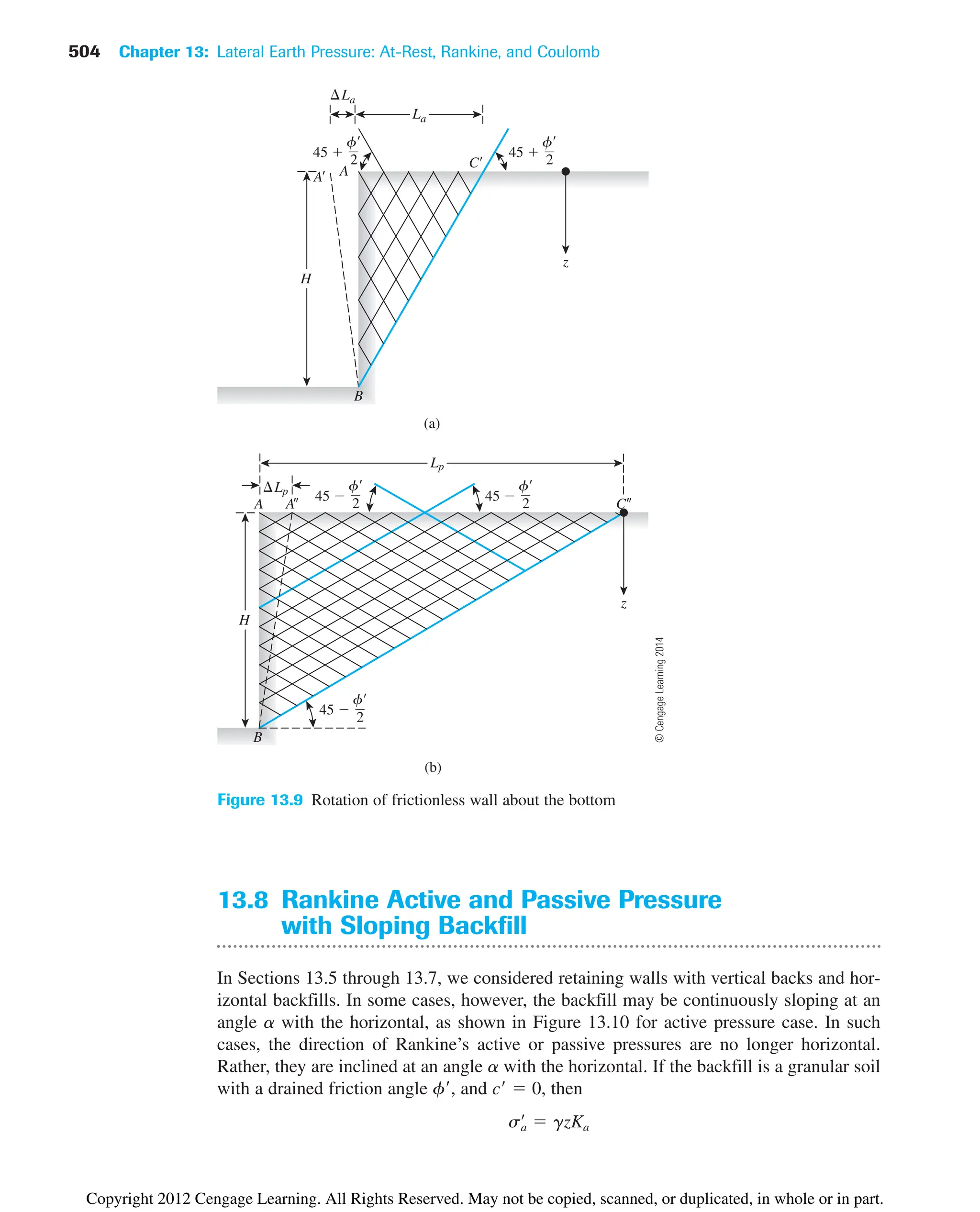
![13.8 Rankine Active and Passive Pressure with Sloping Backfill 505
γ
φ
z
α
α
a
Frictionless
wall
H σ′
c
Figure 13.10
Frictionless vertical retaining wall with
sloping backfill
Table 13.2 Values of Ka [Eq. (13.23)]
F (deg) B
T A (deg) 28 30 32 34 36 38 40
0 0.361 0.333 0.307 0.283 0.260 0.238 0.217
5 0.366 0.337 0.311 0.286 0.262 0.240 0.219
10 0.380 0.350 0.321 0.294 0.270 0.246 0.225
15 0.409 0.373 0.341 0.311 0.283 0.258 0.235
20 0.461 0.414 0.374 0.338 0.306 0.277 0.250
25 0.573 0.494 0.434 0.385 0.343 0.307 0.275
where
(13.23)
The active force per unit length of the wall can be given as
(13.24)
The line of action of the resultant acts at a distance of H/3 measured from the bottom of
the wall. Table 13.2 gives the values of Ka for various combinations of a and f.
In a similar manner, the Rankine passive earth pressure for a wall of height H with
a granular sloping backfill can be represented by the equation
(13.25)
Pp
1
2
gH2
Kp
Pa
1
2
KagH2
cos a
cos a 2 cos 2
a cos 2
fœ
cos a 2 cos 2
a cos 2
fœ
Ka Rankine’s active pressure coefficient
©
Cengage
Learning
2014
©
Cengage
Learning
2014
Copyright 2012 Cengage Learning. All Rights Reserved. May not be copied, scanned, or duplicated, in whole or in part.](https://image.slidesharecdn.com/principlesofgeotechnicalengineering-8thedition-231222125509-7e44d9bf/75/Principles-of-Geotechnical-Engineering-8th-Edition-pdf-525-2048.jpg)
![506 Chapter 13: Lateral Earth Pressure: At-Rest, Rankine, and Coulomb
Table 13.3 Passive Earth Pressure Coefficient, Kp [Eq. (13.26)]
F (deg) B
T A (deg) 28 30 32 34 36 38 40
0 2.770 3.000 3.255 3.537 3.852 4.204 4.599
5 2.715 2.943 3.196 3.476 3.788 4.136 4.527
10 2.551 2.775 3.022 3.295 3.598 3.937 4.316
15 2.284 2.502 2.740 3.003 3.293 3.615 3.977
20 1.918 2.132 2.362 2.612 2.886 3.189 3.526
25 1.434 1.664 1.894 2.135 2.394 2.676 2.987
where
(13.26)
is the passive earth pressure coefficient.
As in the case of the active force, the resultant force Pp is inclined at an angle a with
the horizontal and intersects the wall at a distance of H/3 measured from the bottom of the
wall. The values of Kp (passive earth pressure coefficient) for various values of a and f
are given in Table 13.3.
A generalized case for Rankine active and passive pressure with granular backfill is
given in Appendix A.
13.9 Diagrams for Lateral Earth-Pressure
Distribution against Retaining Walls
Backfill—Cohesionless Soil with Horizontal Ground Surface
Active Case Figure 13.11a shows a retaining wall with cohensionless soil backfill that
has a horizontal ground surface. The unit weight and the angle of friction of the soil are g
and f, respectively.
For Rankine’s active state, the earth pressure at any depth against the retaining wall
can be given by Eq. (13.17):
Note that increases linearly with depth, and at the bottom of the wall, it is
(13.27)
The total force per unit length of the wall is equal to the area of the pressure diagram, so
(13.28)
Pa
1
2
KagH2
sa
œ
KagH
sa
œ
sa
œ
Kagz 1Note: cœ
02
Kp cos a
cos a 2 cos 2
a cos 2
fœ
cos a 2 cos 2
a cos 2
fœ
©
Cengage
Learning
2014
Copyright 2012 Cengage Learning. All Rights Reserved. May not be copied, scanned, or duplicated, in whole or in part.](https://image.slidesharecdn.com/principlesofgeotechnicalengineering-8thedition-231222125509-7e44d9bf/75/Principles-of-Geotechnical-Engineering-8th-Edition-pdf-526-2048.jpg)
![13.9 Diagrams for Lateral Earth-Pressure Distribution against Retaining Walls 507
H
Failure
wedge
g
f
c 0
(a)
sa
Pa
H
3
(b)
KpgH
sp
Pp
H
3
Failure wedge
H
H
H
KagH
f
2
45
f
2
45
g
f
c 0
Figure 13.11
Pressure distribu-
tion against a
retaining wall for
cohensionless soil
backfill with
horizontal ground
surface:
(a) Rankine’s
active state;
(b) Rankine’s
passive state
Passive Case The lateral pressure distribution against a retaining wall of height H for
Rankine’s passive state is shown in Figure 13.11b. The lateral earth pressure at any depth z
[Eq. (13.22), c 0] is
(13.29)
The total force per unit length of the wall is
(13.30)
Backfill—Partially Submerged Cohensionless
Soil Supporting a Surcharge
Active Case Figure 13.12a shows a frictionless retaining wall of height H and a backfill
of cohensionless soil. The groundwater table is located at a depth of H1 below the ground
surface, and the backfill is supporting a surcharge pressure of q per unit area. From
Eq. (13.19), the effective active earth pressure at any depth can be given by
(13.31)
sa
œ
Kaso
œ
Pp
1
2
KpgH2
sp
œ
KpgH
©
Cengage
Learning
2014
Copyright 2012 Cengage Learning. All Rights Reserved. May not be copied, scanned, or duplicated, in whole or in part.](https://image.slidesharecdn.com/principlesofgeotechnicalengineering-8thedition-231222125509-7e44d9bf/75/Principles-of-Geotechnical-Engineering-8th-Edition-pdf-527-2048.jpg)
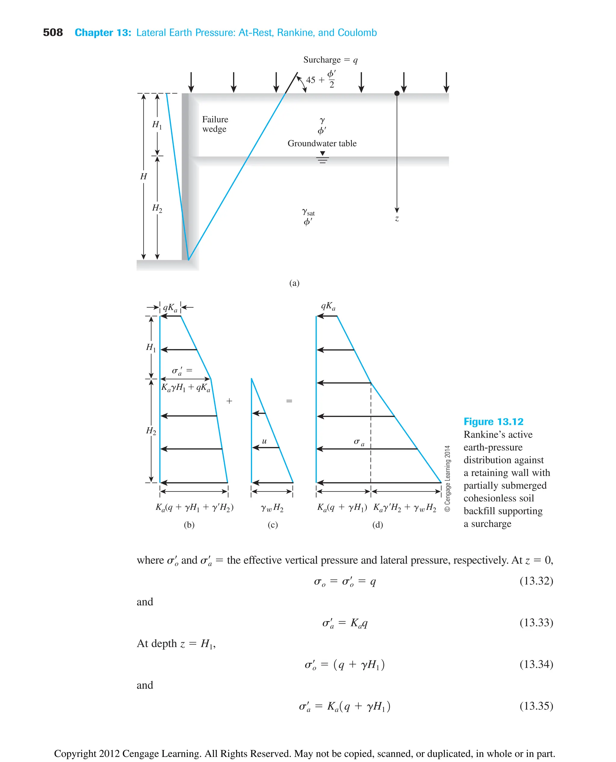
![13.9 Diagrams for Lateral Earth-Pressure Distribution against Retaining Walls 509
At depth z H,
(13.36)
and
(13.37)
where g gsat gw. The variation of with depth is shown in Figure 13.12b.
The lateral pressure on the wall from the pore water between and H1 is 0, and
for z H1, it increases linearly with depth (Figure 13.12c). At ,
The total lateral-pressure diagram (Figure 13.12d) is the sum of the pressure dia-
grams shown in Figures 13.12b and 13.12c. The total active force per unit length of the
wall is the area of the total pressure diagram. Thus,
(13.38)
Passive Case Figure 13.13a shows the same retaining wall as was shown in Figure 13.12a.
Rankine’s passive pressure at any depth against the wall can be given by Eq. (13.22):
Using the preceding equation, we can determine the variation of with depth, as
shown in Figure 13.13b. The variation of the pressure on the wall from water with depth
is shown in Figure 13.13c. Figure 13.13d shows the distribution of the total pressure p
with depth. The total lateral passive force per unit length of the wall is the area of the dia-
gram given in Figure 13.13d, or
(13.39)
Backfill—Cohesive Soil with Horizontal Backfill
Active Case Figure 13.14a shows a frictionless retaining wall with a cohesive soil back-
fill. The active pressure against the wall at any depth below the ground surface can be
expressed as [Eq. (13.17)]
The variation of Kagz with depth is shown in Figure 13.14b, and the variation of
with depth is shown in Figure 13.14c. Note that is not a function of z;
hence, Figure 13.14c is a rectangle. The variation of the net value of with depth is plot-
ted in Figure 13.14d. Also note that, because of the effect of cohesion, is negative in the
upper part of the retaining wall. The depth zo at which the active pressure becomes equal
to 0 can be found from Eq. (13.17) as
Kagzo 21Kacœ
0
sa
œ
sa
œ
21Kacœ
21Kacœ
sa
œ
Kagz 21Kacœ
Pp KpqH
1
2
KpgH1
2
KpgH1H2
1
2
1Kpgœ
gw2H2
2
sp
œ
sp
œ
Kpso
œ
Pa KaqH
1
2
KagH1
2
KagH1H2
1
2
1Kagœ
gw2H2
2
u gwH2
z H
z 0
sa
œ
sa
œ
Ka1q gH1 gœ
H22
so
œ
1q gH1 gœ
H22
Copyright 2012 Cengage Learning. All Rights Reserved. May not be copied, scanned, or duplicated, in whole or in part.](https://image.slidesharecdn.com/principlesofgeotechnicalengineering-8thedition-231222125509-7e44d9bf/75/Principles-of-Geotechnical-Engineering-8th-Edition-pdf-529-2048.jpg)
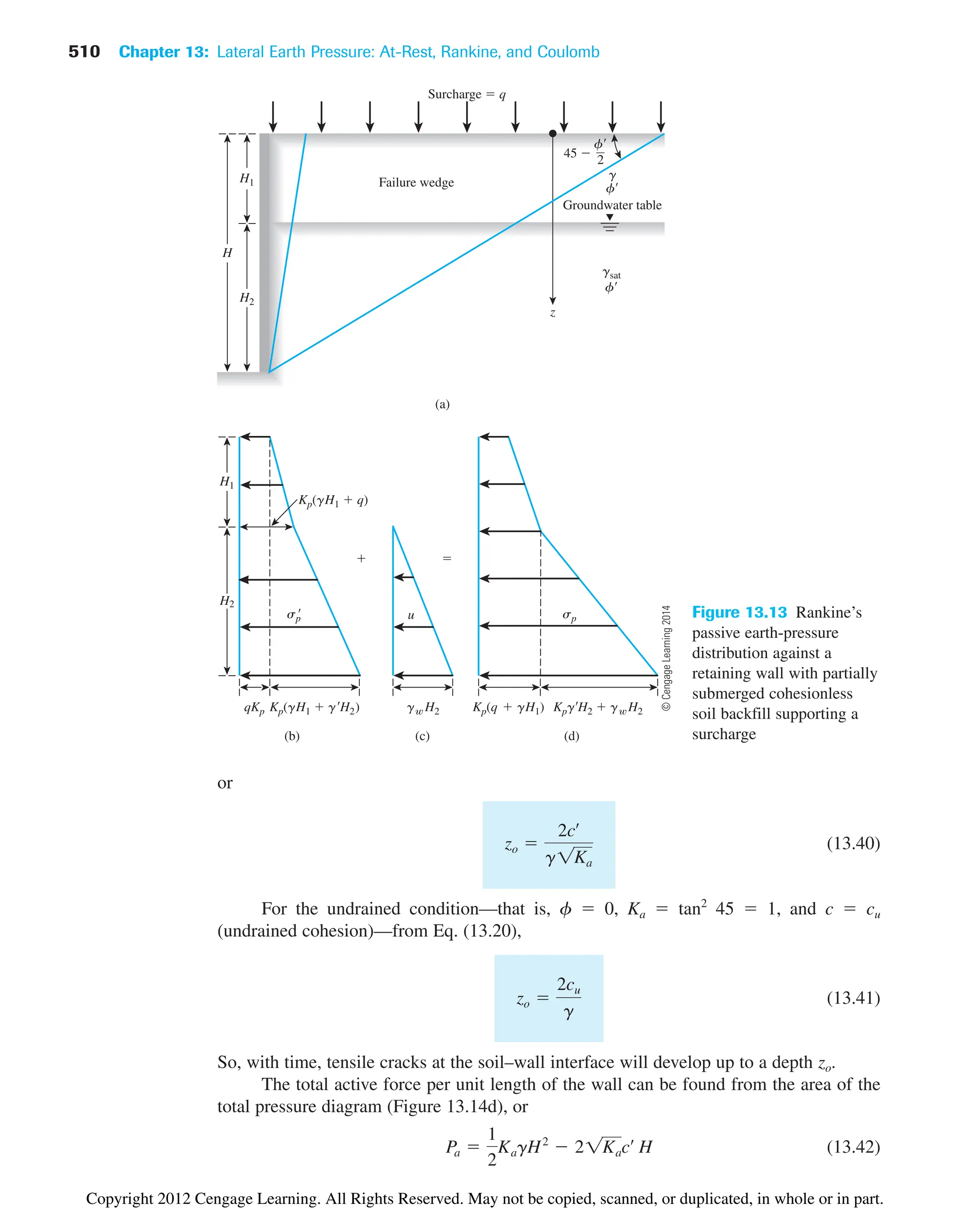
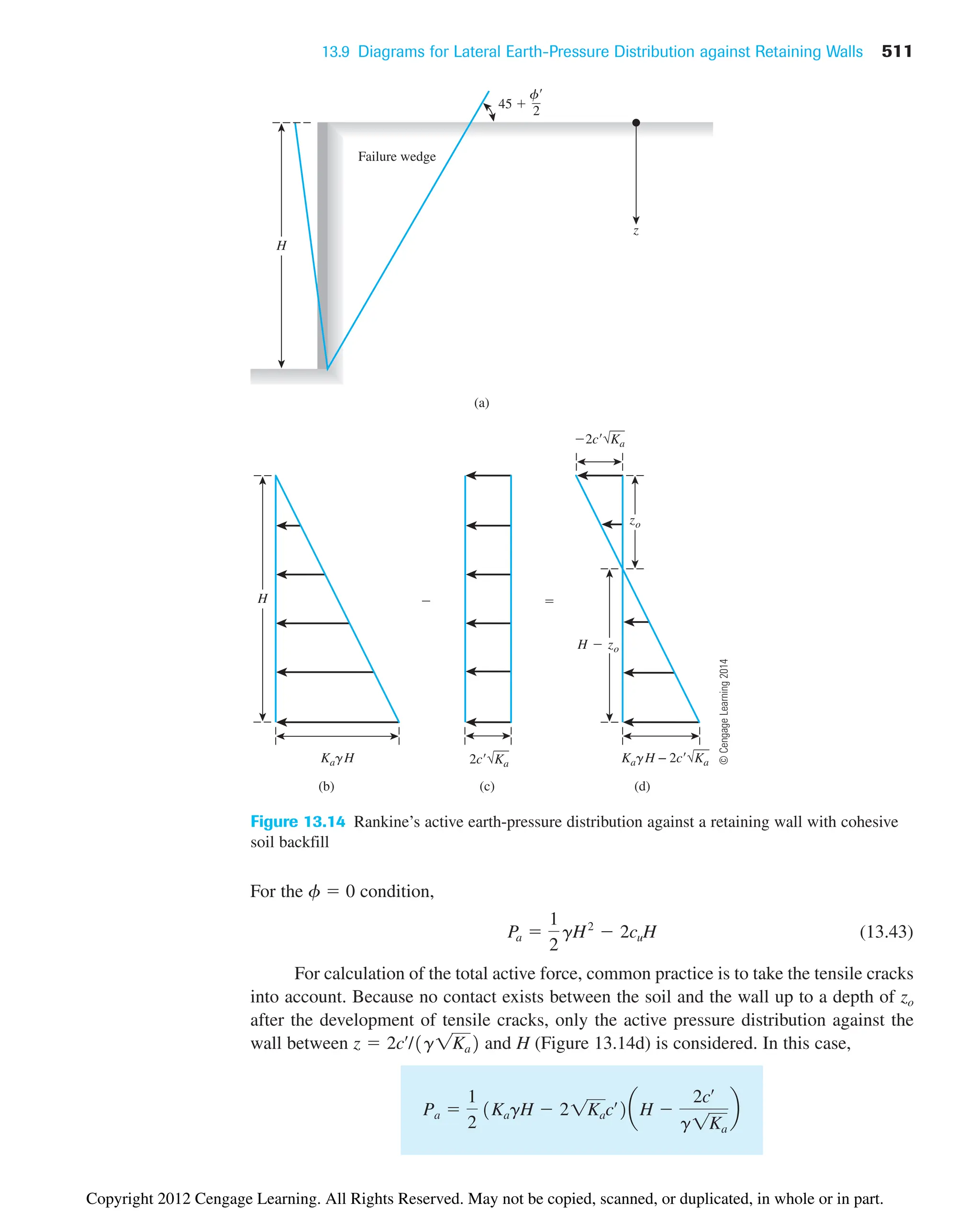
![512 Chapter 13: Lateral Earth Pressure: At-Rest, Rankine, and Coulomb
(a) (b)
2c√Kp KpgH
Failure wedge
sp
H
z
f
2
45
Figure 13.15
Rankine’s passive
earth-pressure
distribution against
a retaining wall
with cohesive soil
backfill
(13.44)
For the f 0 condition,
(13.45)
Passive Case Figure 13.15a shows the same retaining wall with backfill similar to that
considered in Figure 13.14a. Rankine’s passive pressure against the wall at depth z can be
given by [Eq. (13.21)]
At z 0,
(13.46)
and at z H,
(13.47)
The variation of with depth is shown in Figure 13.15b. The passive force per unit
length of the wall can be found from the area of the pressure diagrams as
(13.48a)
For the f 0 condition, Kp 1 and
(13.48b)
Pp
1
2
gH2
2cuH
Pp
1
2
KpgH2
23Kpcœ
H
sp
œ
sp
œ
KpgH 23Kpcœ
sp
œ
23Kpcœ
sp
œ
Kpgz 23Kp cœ
Pa
1
2
gH2
2cuH 2
cu
2
g
1
2
KagH2
21Kacœ
H 2
cœ2
g
©
Cengage
Learning
2014
Copyright 2012 Cengage Learning. All Rights Reserved. May not be copied, scanned, or duplicated, in whole or in part.](https://image.slidesharecdn.com/principlesofgeotechnicalengineering-8thedition-231222125509-7e44d9bf/75/Principles-of-Geotechnical-Engineering-8th-Edition-pdf-532-2048.jpg)
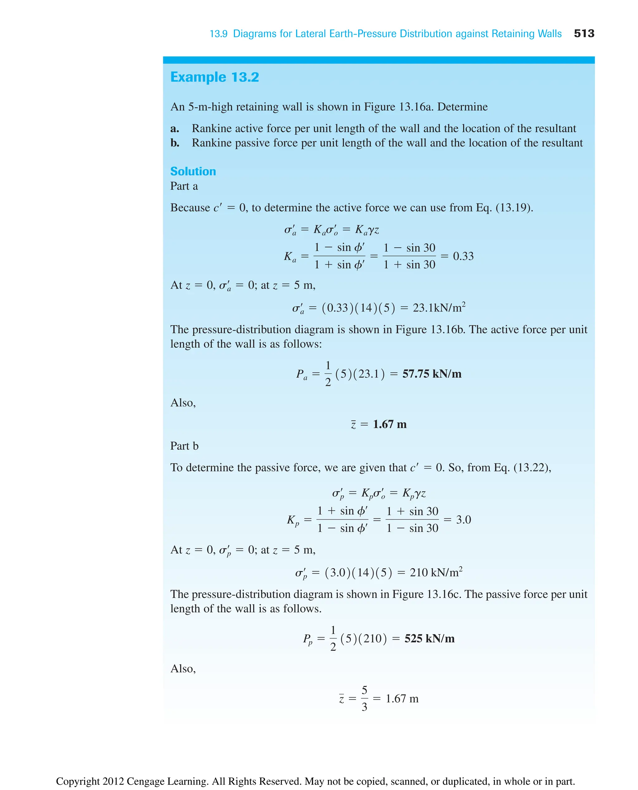
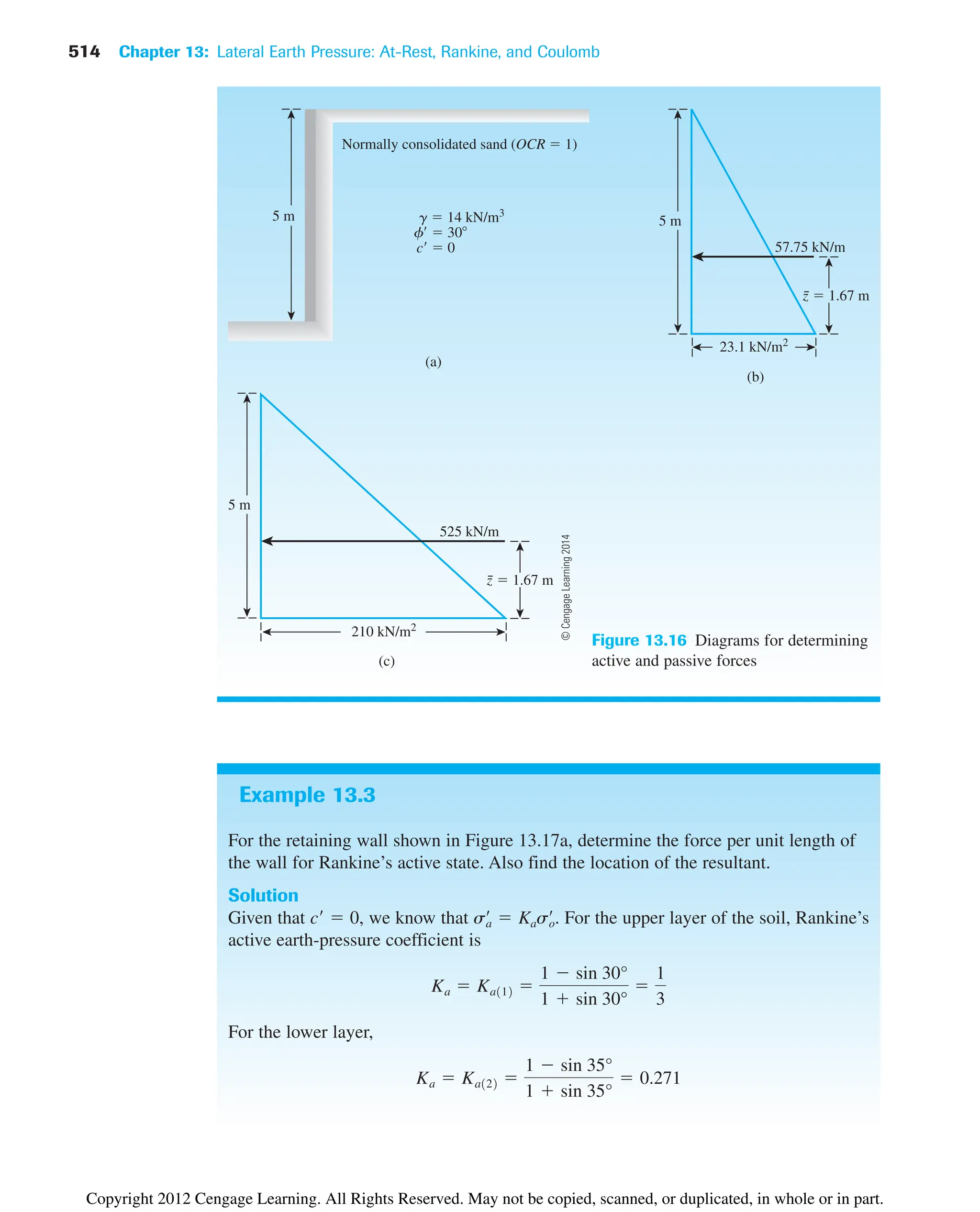
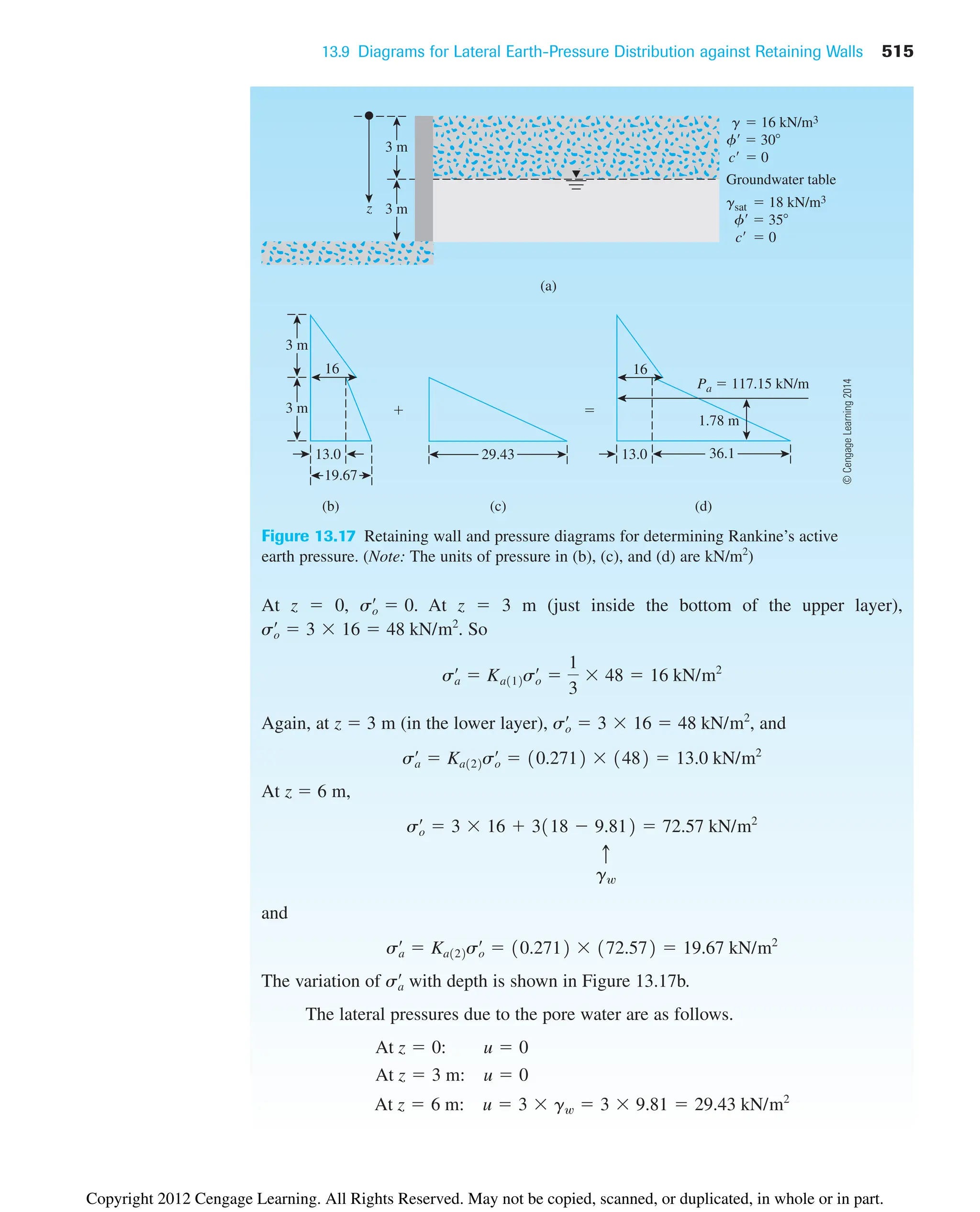
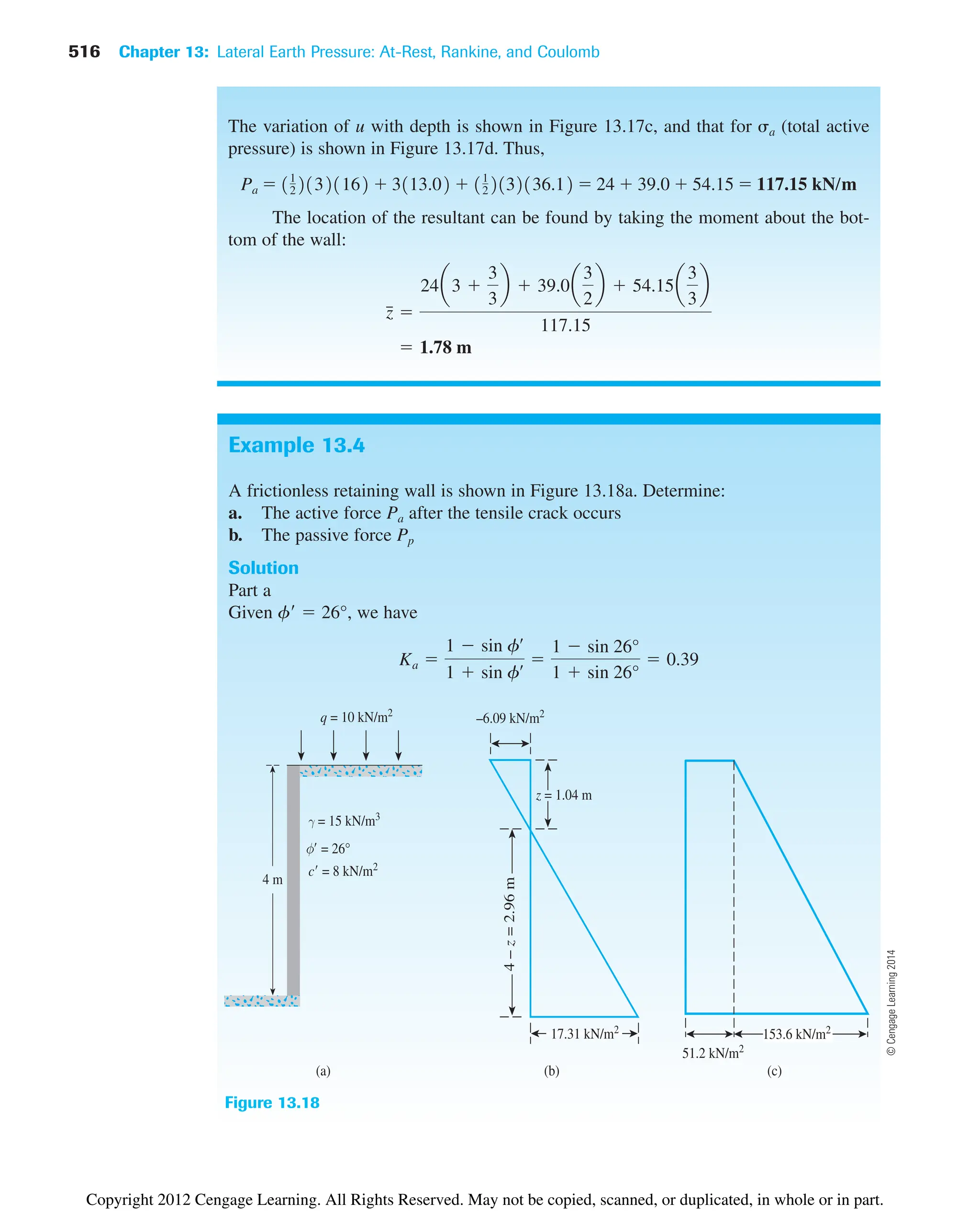
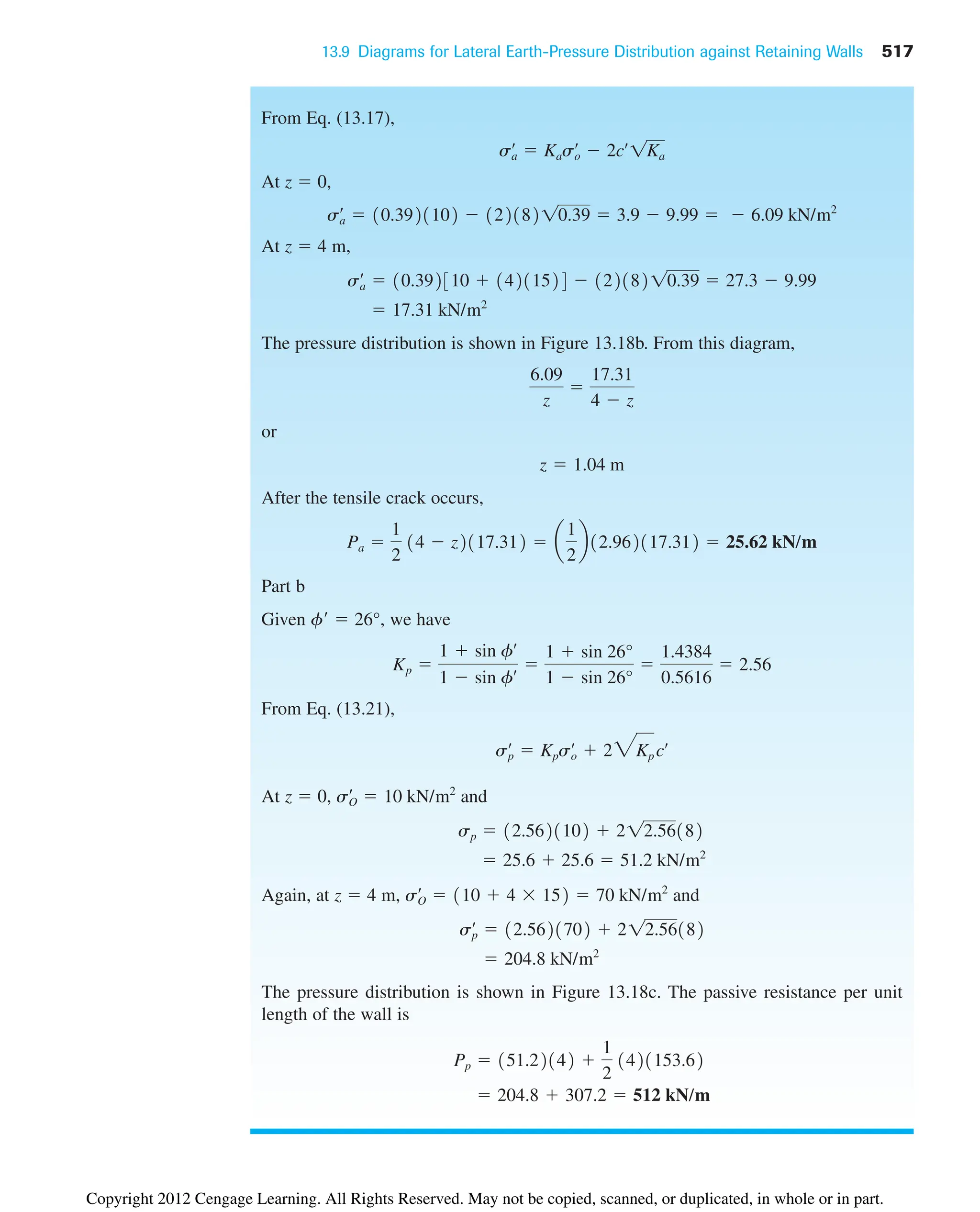
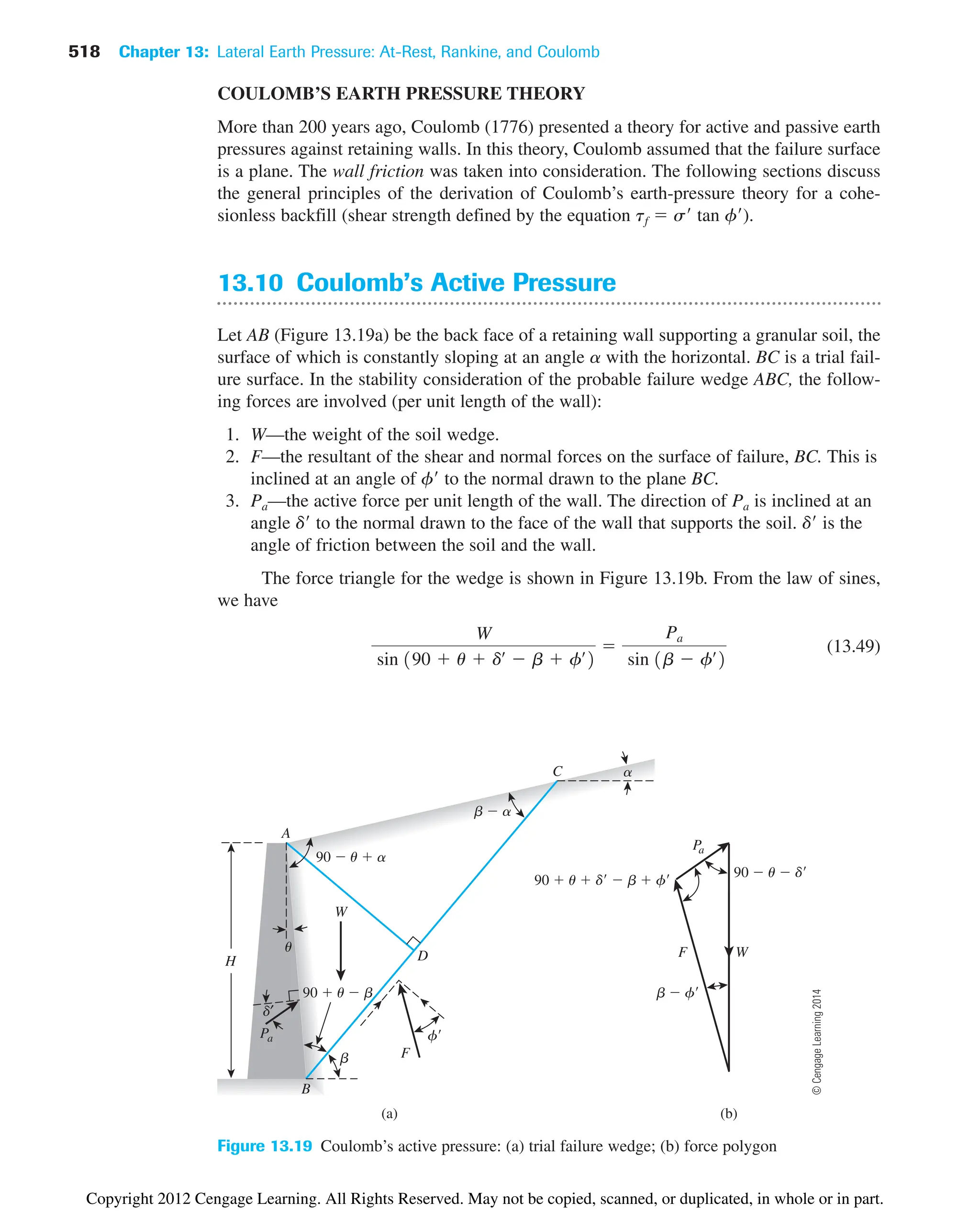
![13.10 Coulomb’s Active Pressure 519
or
(13.50)
The preceding equation can be written in the form
(13.51)
where g unit weight of the backfill. The values of g, H, u, a, f, and d are constants,
and b is the only variable. To determine the critical value of b for maximum Pa, we have
(13.52)
After solving Eq. (13.52), when the relationship of b is substituted into Eq. (13.51),
we obtain Coulomb’s active earth pressure as
(13.53)
where Ka is Coulomb’s active earth-pressure coefficient and is given by
(13.54)
Note that when a 0°, u 0°, and d 0°, Coulomb’s active earth-pressure coef-
ficient becomes equal to (1 sin f)/(1 sin f), which is the same as Rankine’s earth-
pressure coefficient given earlier in this chapter.
The variation of the values of Ka for retaining walls with a vertical back (u 0°) and
horizontal backfill (a 0°) is given in Table 13.4. From this table, note that for a given value
of f, the effect of wall friction is to reduce somewhat the active earth-pressure coefficient.
Tables 13.5 and 13.6 also give the variation of Ka [Eq. (13.54)] for various values of
a, f, u, and d ( Table 13.5 and Table 13.6).
dœ
1
2fœ
in
dœ
2
3fœ
in
Ka
cos 2
1fœ
u2
cos 2
u cos 1dœ
u2c1
D
sin 1dœ
fœ
2 sin 1fœ
a2
cos 1dœ
u2 cos 1u a2
d
2
Pa
1
2
KagH2
dPa
db
0
Pa
1
2
gH2
c
cos 1u b2 cos 1u a2 sin 1b fœ
2
cos 2
u sin 1b a2 sin 190 u dœ
b fœ
2
d
Pa
sin 1b fœ
2
sin 190 u dœ
b fœ
2
W
Table 13.4 Values of Ka [Eq. (13.54)] for u 0°, a 0°
D (deg) B
T F (deg) 0 5 10 15 20 25
28 0.3610 0.3448 0.3330 0.3251 0.3203 0.3186
30 0.3333 0.3189 0.3085 0.3014 0.2973 0.2956
32 0.3073 0.2945 0.2853 0.2791 0.2755 0.2745
34 0.2827 0.2714 0.2633 0.2579 0.2549 0.2542
36 0.2596 0.2497 0.2426 0.2379 0.2354 0.2350
38 0.2379 0.2292 0.2230 0.2190 0.2169 0.2167
40 0.2174 0.2089 0.2045 0.2011 0.1994 0.1995
42 0.1982 0.1916 0.1870 0.1841 0.1828 0.1831
©
Cengage
Learning
2014
Copyright 2012 Cengage Learning. All Rights Reserved. May not be copied, scanned, or duplicated, in whole or in part.](https://image.slidesharecdn.com/principlesofgeotechnicalengineering-8thedition-231222125509-7e44d9bf/75/Principles-of-Geotechnical-Engineering-8th-Edition-pdf-539-2048.jpg)
![520 Chapter 13: Lateral Earth Pressure: At-Rest, Rankine, and Coulomb
Table 13.5 Values of Ka [Eq. (13.54)] (Note: )
U (deg)
A F
(deg) (deg) 0 5 10 15 20 25
0 28 0.3213 0.3588 0.4007 0.4481 0.5026 0.5662
29 0.3091 0.3467 0.3886 0.4362 0.4908 0.5547
30 0.2973 0.3349 0.3769 0.4245 0.4794 0.5435
31 0.2860 0.3235 0.3655 0.4133 0.4682 0.5326
32 0.2750 0.3125 0.3545 0.4023 0.4574 0.5220
33 0.2645 0.3019 0.3439 0.3917 0.4469 0.5117
34 0.2543 0.2916 0.3335 0.3813 0.4367 0.5017
35 0.2444 0.2816 0.3235 0.3713 0.4267 0.4919
36 0.2349 0.2719 0.3137 0.3615 0.4170 0.4824
37 0.2257 0.2626 0.3042 0.3520 0.4075 0.4732
38 0.2168 0.2535 0.2950 0.3427 0.3983 0.4641
39 0.2082 0.2447 0.2861 0.3337 0.3894 0.4553
40 0.1998 0.2361 0.2774 0.3249 0.3806 0.4468
41 0.1918 0.2278 0.2689 0.3164 0.3721 0.4384
42 0.1840 0.2197 0.2606 0.3080 0.3637 0.4302
5 28 0.3431 0.3845 0.4311 0.4843 0.5461 0.6190
29 0.3295 0.3709 0.4175 0.4707 0.5325 0.6056
30 0.3165 0.3578 0.4043 0.4575 0.5194 0.5926
31 0.3039 0.3451 0.3916 0.4447 0.5067 0.5800
32 0.2919 0.3329 0.3792 0.4324 0.4943 0.5677
33 0.2803 0.3211 0.3673 0.4204 0.4823 0.5558
34 0.2691 0.3097 0.3558 0.4088 0.4707 0.5443
35 0.2583 0.2987 0.3446 0.3975 0.4594 0.5330
36 0.2479 0.2881 0.3338 0.3866 0.4484 0.5221
37 0.2379 0.2778 0.3233 0.3759 0.4377 0.5115
38 0.2282 0.2679 0.3131 0.3656 0.4273 0.5012
39 0.2188 0.2582 0.3033 0.3556 0.4172 0.4911
40 0.2098 0.2489 0.2937 0.3458 0.4074 0.4813
41 0.2011 0.2398 0.2844 0.3363 0.3978 0.4718
42 0.1927 0.2311 0.2753 0.3271 0.3884 0.4625
10 28 0.3702 0.4164 0.4686 0.5287 0.5992 0.6834
29 0.3548 0.4007 0.4528 0.5128 0.5831 0.6672
30 0.3400 0.3857 0.4376 0.4974 0.5676 0.6516
31 0.3259 0.3713 0.4230 0.4826 0.5526 0.6365
32 0.3123 0.3575 0.4089 0.4683 0.5382 0.6219
33 0.2993 0.3442 0.3953 0.4545 0.5242 0.6078
34 0.2868 0.3314 0.3822 0.4412 0.5107 0.5942
35 0.2748 0.3190 0.3696 0.4283 0.4976 0.5810
36 0.2633 0.3072 0.3574 0.4158 0.4849 0.5682
37 0.2522 0.2957 0.3456 0.4037 0.4726 0.5558
38 0.2415 0.2846 0.3342 0.3920 0.4607 0.5437
39 0.2313 0.2740 0.3231 0.3807 0.4491 0.5321
40 0.2214 0.2636 0.3125 0.3697 0.4379 0.5207
41 0.2119 0.2537 0.3021 0.3590 0.4270 0.5097
42 0.2027 0.2441 0.2921 0.3487 0.4164 0.4990
dœ
2
3 fœ
©
Cengage
Learning
2014
Copyright 2012 Cengage Learning. All Rights Reserved. May not be copied, scanned, or duplicated, in whole or in part.](https://image.slidesharecdn.com/principlesofgeotechnicalengineering-8thedition-231222125509-7e44d9bf/75/Principles-of-Geotechnical-Engineering-8th-Edition-pdf-540-2048.jpg)
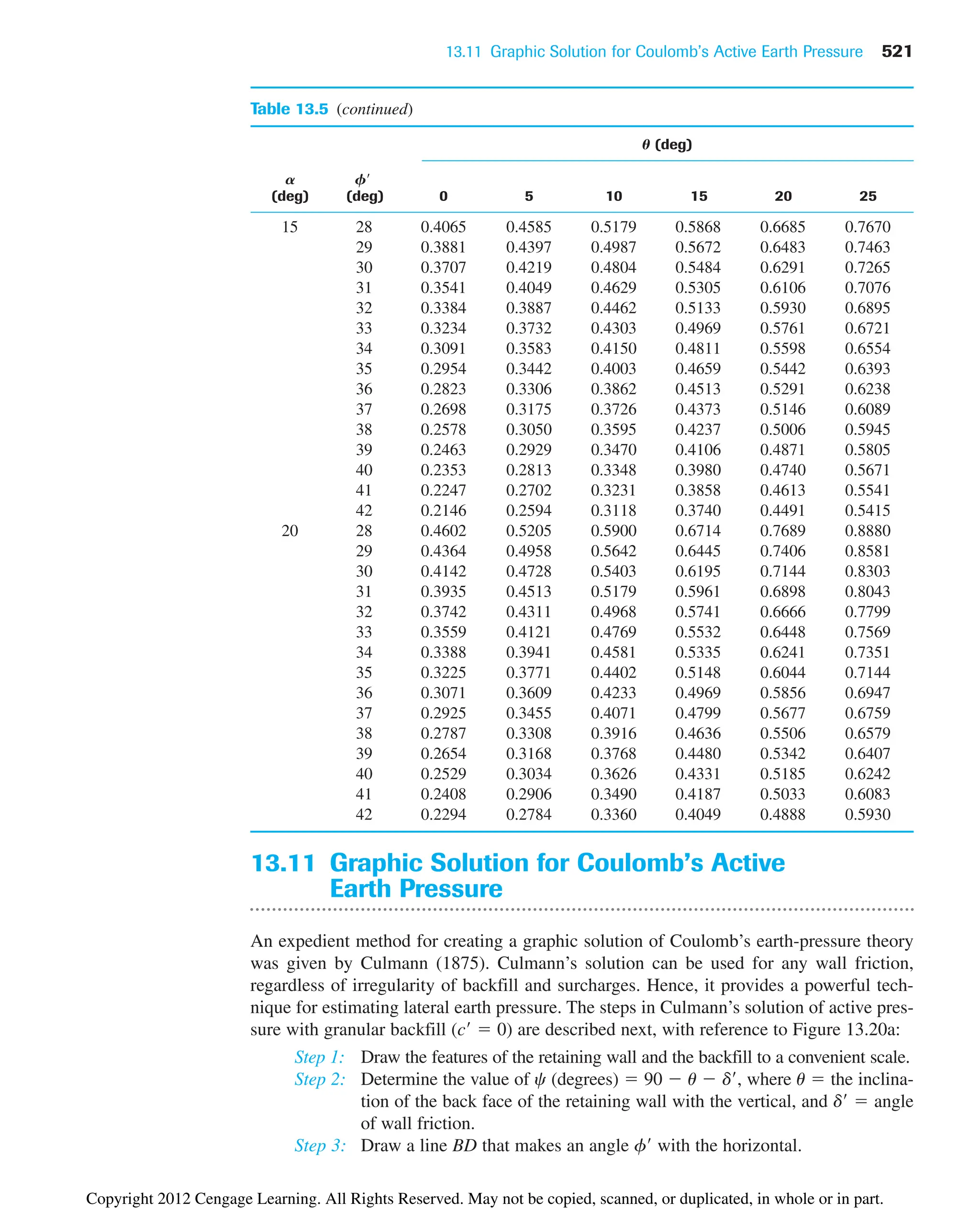
![522 Chapter 13: Lateral Earth Pressure: At-Rest, Rankine, and Coulomb
Table 13.6 Values of Ka [Eq. (13.54)] (Note: d f/2)
U (deg)
A F
(deg) (deg) 0 5 10 15 20 25
0 28 0.3264 0.3629 0.4034 0.4490 0.5011 0.5616
29 0.3137 0.3502 0.3907 0.4363 0.4886 0.5492
30 0.3014 0.3379 0.3784 0.4241 0.4764 0.5371
31 0.2896 0.3260 0.3665 0.4121 0.4645 0.5253
32 0.2782 0.3145 0.3549 0.4005 0.4529 0.5137
33 0.2671 0.3033 0.3436 0.3892 0.4415 0.5025
34 0.2564 0.2925 0.3327 0.3782 0.4305 0.4915
35 0.2461 0.2820 0.3221 0.3675 0.4197 0.4807
36 0.2362 0.2718 0.3118 0.3571 0.4092 0.4702
37 0.2265 0.2620 0.3017 0.3469 0.3990 0.4599
38 0.2172 0.2524 0.2920 0.3370 0.3890 0.4498
39 0.2081 0.2431 0.2825 0.3273 0.3792 0.4400
40 0.1994 0.2341 0.2732 0.3179 0.3696 0.4304
41 0.1909 0.2253 0.2642 0.3087 0.3602 0.4209
42 0.1828 0.2168 0.2554 0.2997 0.3511 0.4117
5 28 0.3477 0.3879 0.4327 0.4837 0.5425 0.6115
29 0.3337 0.3737 0.4185 0.4694 0.5282 0.5972
30 0.3202 0.3601 0.4048 0.4556 0.5144 0.5833
31 0.3072 0.3470 0.3915 0.4422 0.5009 0.5698
32 0.2946 0.3342 0.3787 0.4292 0.4878 0.5566
33 0.2825 0.3219 0.3662 0.4166 0.4750 0.5437
34 0.2709 0.3101 0.3541 0.4043 0.4626 0.5312
35 0.2596 0.2986 0.3424 0.3924 0.4505 0.5190
36 0.2488 0.2874 0.3310 0.3808 0.4387 0.5070
37 0.2383 0.2767 0.3199 0.3695 0.4272 0.4954
38 0.2282 0.2662 0.3092 0.3585 0.4160 0.4840
39 0.2185 0.2561 0.2988 0.3478 0.4050 0.4729
40 0.2090 0.2463 0.2887 0.3374 0.3944 0.4620
41 0.1999 0.2368 0.2788 0.3273 0.3840 0.4514
42 0.1911 0.2276 0.2693 0.3174 0.3738 0.4410
10 28 0.3743 0.4187 0.4688 0.5261 0.5928 0.6719
29 0.3584 0.4026 0.4525 0.5096 0.5761 0.6549
30 0.3432 0.3872 0.4368 0.4936 0.5599 0.6385
31 0.3286 0.3723 0.4217 0.4782 0.5442 0.6225
32 0.3145 0.3580 0.4071 0.4633 0.5290 0.6071
33 0.3011 0.3442 0.3930 0.4489 0.5143 0.5920
34 0.2881 0.3309 0.3793 0.4350 0.5000 0.5775
35 0.2757 0.3181 0.3662 0.4215 0.4862 0.5633
36 0.2637 0.3058 0.3534 0.4084 0.4727 0.5495
37 0.2522 0.2938 0.3411 0.3957 0.4597 0.5361
38 0.2412 0.2823 0.3292 0.3833 0.4470 0.5230
39 0.2305 0.2712 0.3176 0.3714 0.4346 0.5103
40 0.2202 0.2604 0.3064 0.3597 0.4226 0.4979
41 0.2103 0.2500 0.2956 0.3484 0.4109 0.4858
42 0.2007 0.2400 0.2850 0.3375 0.3995 0.4740
©
Cengage
Learning
2014
Copyright 2012 Cengage Learning. All Rights Reserved. May not be copied, scanned, or duplicated, in whole or in part.](https://image.slidesharecdn.com/principlesofgeotechnicalengineering-8thedition-231222125509-7e44d9bf/75/Principles-of-Geotechnical-Engineering-8th-Edition-pdf-542-2048.jpg)
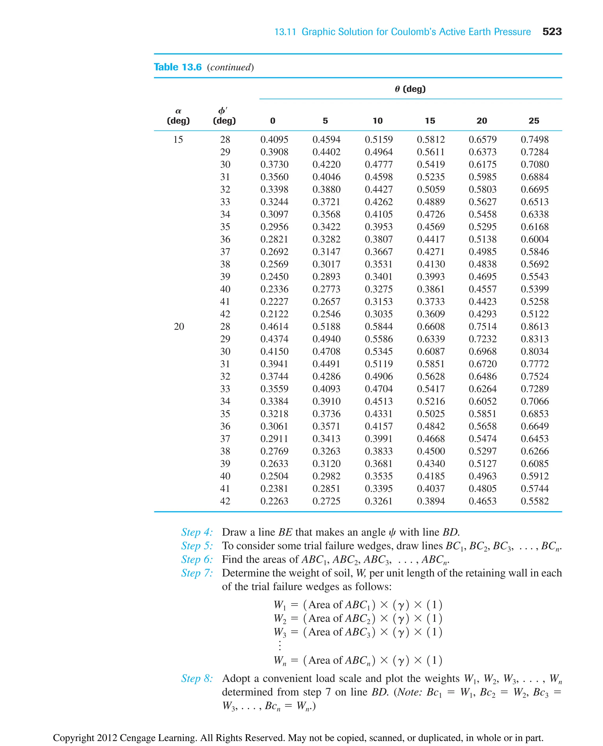
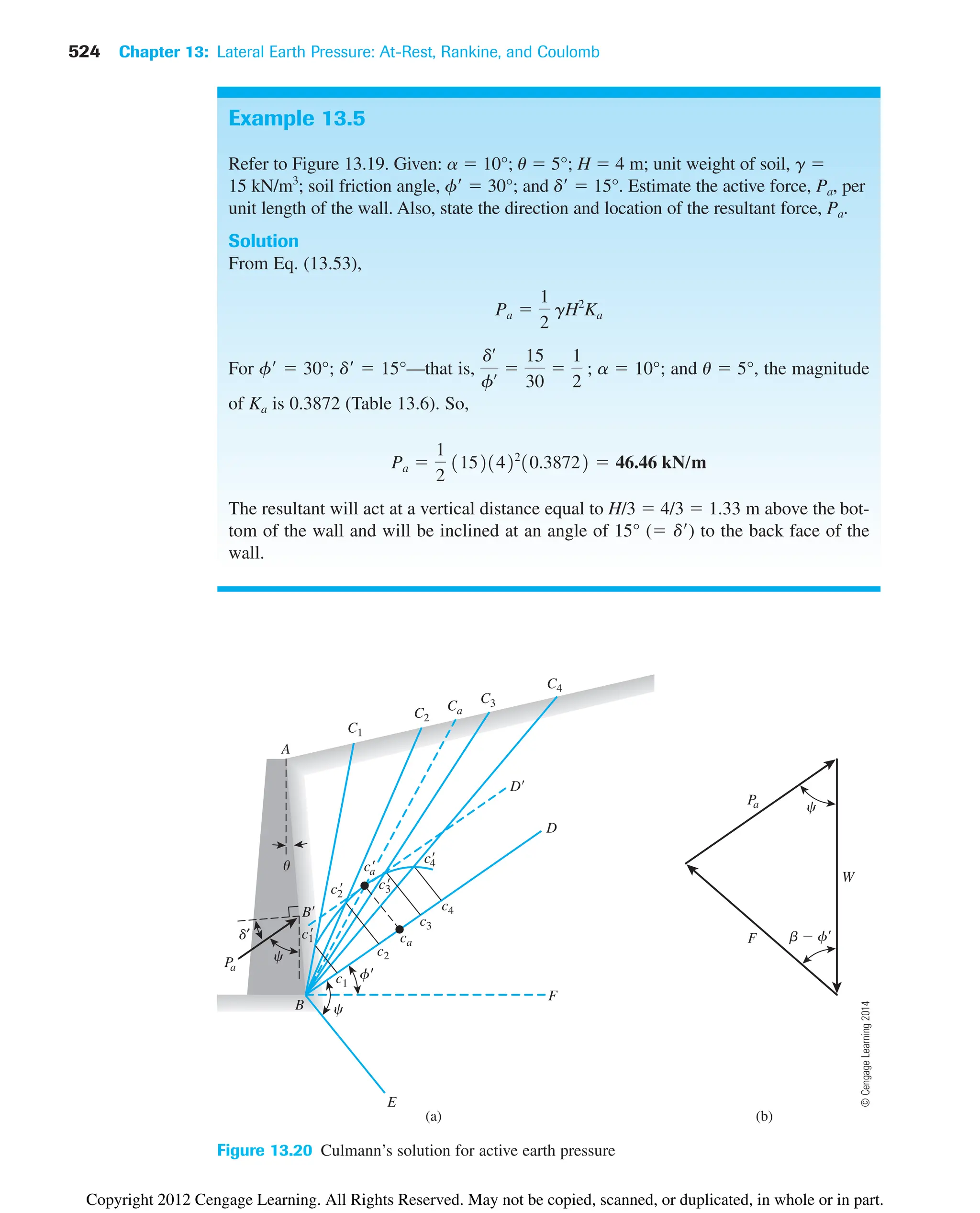
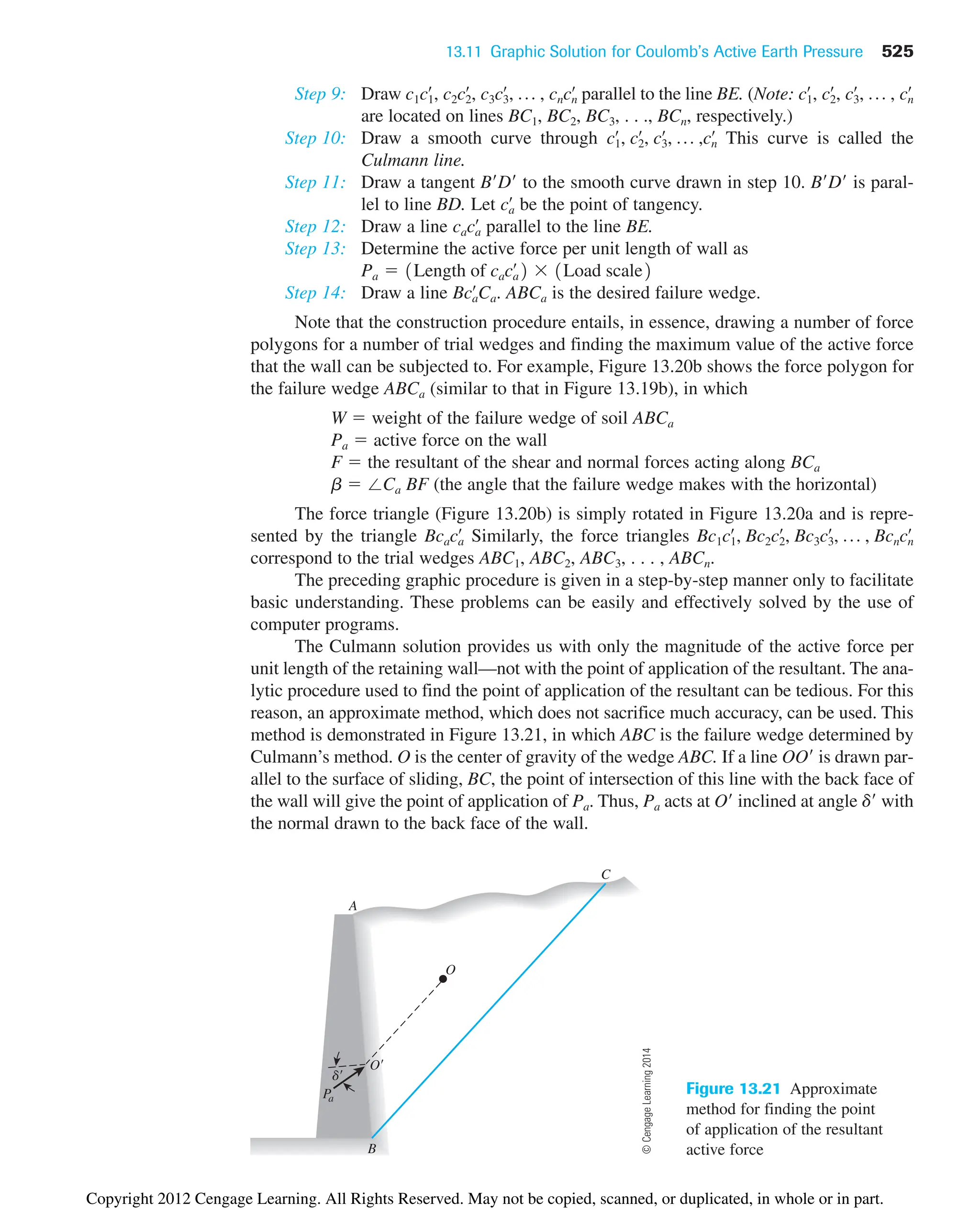
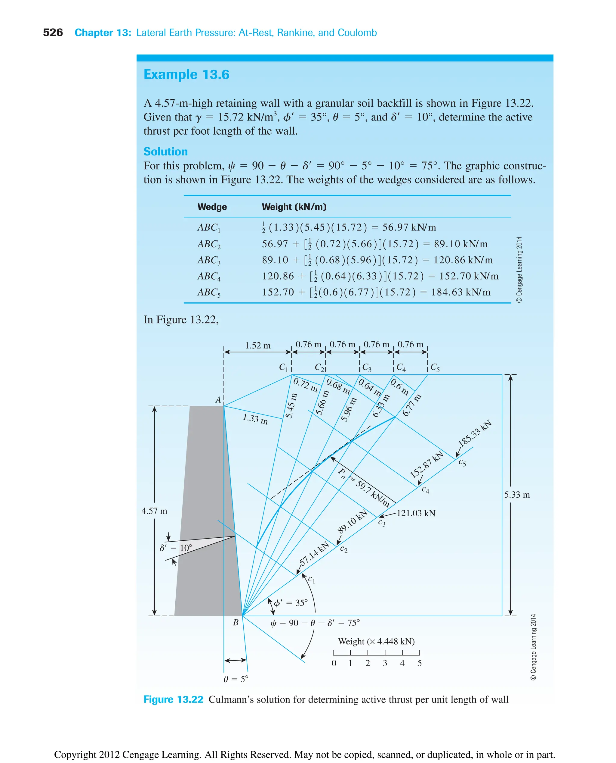
![13.13 Active Force on Retaining Walls with Earthquake Forces 527
13.12 Coulomb’s Passive Pressure
Figure 13.23a shows a retaining wall with a sloping cohensionless backfill similar to that
considered in Figure 13.19a. The force polygon for equilibrium of the wedge ABC for the
passive state is shown in Figure 13.23b. Pp is the notation for the passive force. Other nota-
tions used are the same as those for the active case (Section 13.10). In a procedure similar
to the one that we followed in the active case [Eq. (13.53)], we get
(13.55)
where Kp Coulomb’s passive earth-pressure coefficient, or
(13.56)
For a frictionless wall with the vertical back face supporting granular soil backfill
with a horizontal surface (that is, u 0°, a 0°, and d 0°), Eq. (13.56) yields
This relationship is the same as that obtained for the passive earth-pressure coefficient in
Rankine’s case, given by Eq. (13.22).
The variation of Kp with f and d (for u 0° and a 0°) is given in Table 13.7. We can
see from this table that for given value of f, the value of Kp increases with the wall friction.
13.13 Active Force on Retaining Walls
with Earthquake Forces
Active Case (Granular Backfill)
Coulomb’s analysis for active force on retaining walls discussed in Section 13.10 can be
conveniently extended to include earthquake forces. To do so, let us consider a retaining
wall of height H with a sloping granular backfill, as shown in Figure 13.24a. Let the unit
Kp
1 sin fœ
1 sin fœ tan 2
a45
fœ
2
b
Kp
cos 2
1fœ
u2
cos 2
u cos 1dœ
u2c1
D
sin 1fœ
dœ
2 sin 1fœ
a2
cos 1dœ
u2 cos 1a u2
d
2
Pp 1
2KpgH2
The active thrust per unit length of the wall is 59.7 kN.
Bc5 184.63 kN
Bc4 152.70 kN
Bc3 120.86 kN
Bc2 89.10 kN
Bc1 56.97 kN
Copyright 2012 Cengage Learning. All Rights Reserved. May not be copied, scanned, or duplicated, in whole or in part.](https://image.slidesharecdn.com/principlesofgeotechnicalengineering-8thedition-231222125509-7e44d9bf/75/Principles-of-Geotechnical-Engineering-8th-Edition-pdf-547-2048.jpg)
![528 Chapter 13: Lateral Earth Pressure: At-Rest, Rankine, and Coulomb
H
(a)
B
b
90 u b
P
p
d
W
F
f
u
90 u a
A
C a
[180 (90 u d) (b f)]
(b)
F
W
Pp
90 u d
b f
Figure 13.23 Coulomb’s passive pressure: (a) trial failure wedge; (b) force polygon
Table 13.7 Values of Kp [Eq. 13.56] for u 0°, a 0°
D (deg) B
T F (deg) 0 5 10 15 20
15 1.698 1.900 2.130 2.405 2.735
20 2.040 2.313 2.636 3.030 3.525
25 2.464 2.830 3.286 3.855 4.597
30 3.000 3.506 4.143 4.977 6.105
35 3.690 4.390 5.310 6.854 8.324
40 4.600 5.590 6.946 8.870 11.772
©
Cengage
Learning
2014
©
Cengage
Learning
2014
Copyright 2012 Cengage Learning. All Rights Reserved. May not be copied, scanned, or duplicated, in whole or in part.](https://image.slidesharecdn.com/principlesofgeotechnicalengineering-8thedition-231222125509-7e44d9bf/75/Principles-of-Geotechnical-Engineering-8th-Edition-pdf-548-2048.jpg)
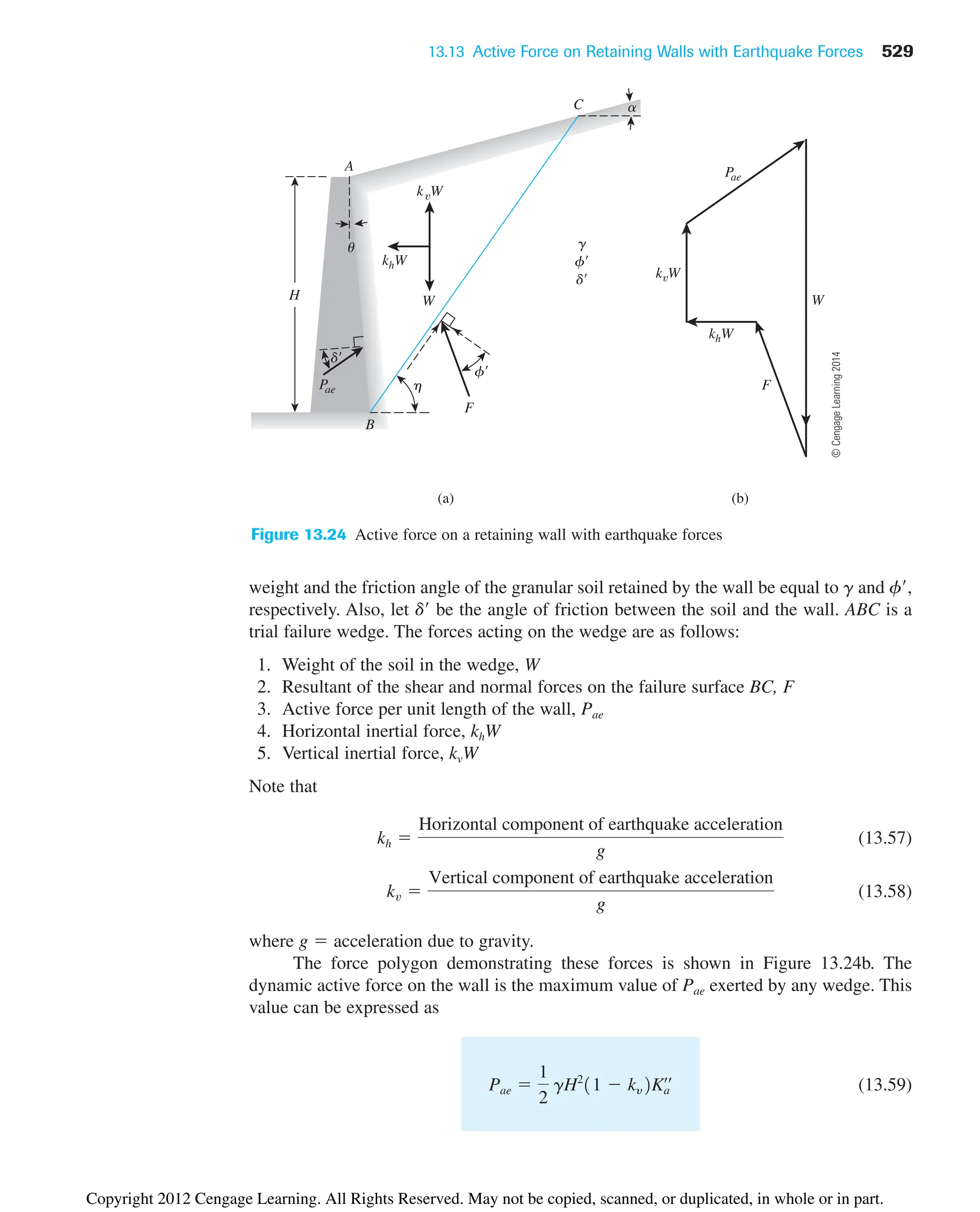
![530 Chapter 13: Lateral Earth Pressure: At-Rest, Rankine, and Coulomb
where
(13.60)
and
(13.61)
Note that with no inertia forces from earthquakes, is equal to 0. Hence, as
given in Eq. (13.54). Equations (13.59) and (13.60) generally are referred to as the
Mononobe–Okabe equations (Mononobe, 1929; Okabe, 1926). The variation of with
Ka
œœ
Ka
œœ
Ka
b
b tan1
a
kh
1 kv
b
Ka
œœ
cos 2
1fœ
u b2
cos2
ucosb cos1dœ
u b2e1 c
sin1dœ
fœ
2sin1fœ
a b2
cos1dœ
ub2cos1ua2
d
1/2
f
2
(for u 0, a 0, 0, f 30°) for which the maximum value of Pae is obtained.
Seed and Whitman (1970) provided a simple procedure to obtain the value of
from the standard charts of [see Eq. (13.54)]. This procedure is explained next.
Referring to Eqs. (13.53) and (13.54), we can write
(13.62)
where
(13.63)
Now, referring to Eqs. (13.59) and (13.60), we can write
(13.64)
where
(13.65)
Now, let us define
(13.66)
and
(13.67)
a* a b
u* u b
cos 2
1fœ
u b2
cos1dœ
u b
2c1
B
sin 1d¿ f¿2 sin 1f¿ a b2
cos 1d¿ u b2 cos 1u a2
d
2
Am Ka
œœ
cos 2
u cos b
Pae
1
2
gH 2
11 kv2Ka
œœ
a
1
2
gH 2
b11 kv2a
1
cos 2
u cos b
b1Am2
Ac Ka cos 2
u
cos 2
1fœ
u2
cos 2
1dœ
u2c1
D
sin 1dœ
fœ
2 sin 1fœ
a2
cos 1dœ
u2 cos 1u a2
d
2
Pa
1
2
gH2
Ka a
1
2
gH2
b a
1
cos 2
u
b1Ac2
Ka
Ka
œœ
kv
u 0° and 0 is given in Table 13.8. Figure 13.25 shows the critical values of h hc
kv
Copyright 2012 Cengage Learning. All Rights Reserved. May not be copied, scanned, or duplicated, in whole or in part.](https://image.slidesharecdn.com/principlesofgeotechnicalengineering-8thedition-231222125509-7e44d9bf/75/Principles-of-Geotechnical-Engineering-8th-Edition-pdf-550-2048.jpg)
![Table 13.8 Values of [Eq. (13.60)] with u 0° and 0
F (deg)
kh D (deg) A (deg) 28 30 35 40 45
0.1 0 0 0.427 0.397 0.328 0.268 0.217
0.2 0.508 0.473 0.396 0.382 0.270
0.3 0.611 0.569 0.478 0.400 0.334
0.4 0.753 0.697 0.581 0.488 0.409
0.5 1.005 0.890 0.716 0.596 0.500
0.1 0 5 0.457 0.423 0.347 0.282 0.227
0.2 0.554 0.514 0.424 0.349 0.285
0.3 0.690 0.635 0.522 0.431 0.356
0.4 0.942 0.825 0.653 0.535 0.442
0.5 — — 0.855 0.673 0.551
0.1 0 10 0.497 0.457 0.371 0.299 0.238
0.2 0.623 0.570 0.461 0.375 0.303
0.3 0.856 0.748 0.585 0.472 0.383
0.4 — — 0.780 0.604 0.486
0.5 — — — 0.809 0.624
0.1 f/2 0 0.396 0.368 0.306 0.253 0.207
0.2 0.485 0.452 0.380 0.319 0.267
0.3 0.604 0.563 0.474 0.402 0.340
0.4 0.778 0.718 0.599 0.508 0.433
0.5 1.115 0.972 0.774 0.648 0.552
0.1 f/2 5 0.428 0.396 0.326 0.268 0.218
0.2 0.537 0.497 0.412 0.342 0.283
0.3 0.699 0.640 0.526 0.438 0.367
0.4 1.025 0.881 0.690 0.568 0.475
0.5 — — 0.962 0.752 0.620
0.1 f/2 10 0.472 0.433 0.352 0.285 0.230
0.2 0.616 0.562 0.454 0.371 0.303
0.3 0.908 0.780 0.602 0.487 0.400
0.4 — — 0.857 0.656 0.531
0.5 — — — 0.944 0.722
0.1 0 0.393 0.366 0.306 0.256 0.212
0.2 0.486 0.454 0.384 0.326 0.276
0.3 0.612 0.572 0.486 0.416 0.357
0.4 0.801 0.740 0.622 0.533 0.462
0.5 1.177 1.023 0.819 0.693 0.600
0.1 5 0.427 0.395 0.327 0.271 0.224
0.2 0.541 0.501 0.418 0.350 0.294
0.3 0.714 0.655 0.541 0.455 0.386
0.4 1.073 0.921 0.722 0.600 0.509
0.5 — — 1.034 0.812 0.679
0.1 10 0.472 0.434 0.354 0.290 0.237
0.2 0.625 0.570 0.463 0.381 0.317
0.3 0.942 0.807 0.624 0.509 0.423
0.4 — — 0.909 0.699 0.573
0.5 — — — 1.037 0.800
2
3
fœ
2
3
fœ
2
3
fœ
kv
Ka
œœ
531
©
Cengage
Learning
2014
Copyright 2012 Cengage Learning. All Rights Reserved. May not be copied, scanned, or duplicated, in whole or in part.](https://image.slidesharecdn.com/principlesofgeotechnicalengineering-8thedition-231222125509-7e44d9bf/75/Principles-of-Geotechnical-Engineering-8th-Edition-pdf-551-2048.jpg)
![532 Chapter 13: Lateral Earth Pressure: At-Rest, Rankine, and Coulomb
0.1
20
30
40 δ′ = 20°
δ′ = 0°
50
η
c
(deg)
60
0.2 0.3 0.4 0.5
kh
kυ = 0
θ = 0
α = 0
φ′ = 30°
0
Figure 13.25 Plot of for 0, u 0, a 0, and f 30°
kv
h hc
Substituting Eqs. (13.66) and (13.67) into the relationship for Am [that is, Eq. (13.65)],
we obtain
(13.68)
Comparing Eqs. (13.63) and (13.68), we have
(13.69)
Hence,
or
(13.70)
The term Pa(u*
, a*
) in Eq. (13.70) is the active earth pressure on an imaginary retain-
ing wall with a wall inclination of u*
and backfill slope inclination of a*
. The value of Ka
can be obtained from standard charts or tables, such as Tables 13.5 and 13.6.
Considering the active force relation given by Eqs. (13.59) through (13.61), we find
that the term sin in Eq. (13.60) has two important implications. First, if
(i.e., negative), no real solution of is possible. Physically, this implies
Ka
œœ
fœ
a b 0
1fœ
a b2
3Pa1u*, a*2411 kv2c
cos 2
1u b2
cos 2
u cos b
d
Pae 3Pa1u*, a*2411 kv2a
cos 2
u*
cos 2
u cos b
b
Pae
1
2
gH2
11 kv2
1
cos 2
u cos b
Ka1u*, a*2 cos 2
u*
Am Ac1u*, a*2 Ka1u*, a*2 cos 2
u*
Am
cos2
1f
œ
u*
2
cos1d
œ
u*
2c1
B
sin1d
œ
f¿
2 sin1f¿
a*
2
cos1d
œ
u*
2 cos1u*
a*
2
d
2
©
Cengage
Learning
2014
Copyright 2012 Cengage Learning. All Rights Reserved. May not be copied, scanned, or duplicated, in whole or in part.](https://image.slidesharecdn.com/principlesofgeotechnicalengineering-8thedition-231222125509-7e44d9bf/75/Principles-of-Geotechnical-Engineering-8th-Edition-pdf-552-2048.jpg)
![13.13 Active Force on Retaining Walls with Earthquake Forces 533
that an equilibrium condition will not exist. Hence, for stability, the limiting slope of the
backfill may be given as
(13.71)
For no earthquake condition, for stability, Eq. (13.71) gives the familiar relation
(13.72)
Second, for horizontal backfill, a 0°; for stability,
(13.73)
Because for stability, combining Eqs. (13.61) and (13.73)
results in
(13.74)
Hence, the critical value of the horizontal acceleration can be defined as
(13.75)
where kh(cr) critical value of horizontal acceleration (Figure 13.26).
Location of Line of Action of Resultant Force, Pae
Seed and Whitman (1970) proposed a simple procedure to determine the location of the
line of action of the resultant, Pae. Their method is as follows:
1. Let
(13.76)
where Pa Coulomb’s active force as determined from Eq. (13.53)
DPae additional active force caused by the earthquake effect
Pae Pa ¢Pae
kh1cr2 11 ky2 tan fœ
kh 11 ky2 tan fœ
b tan 1
3kh/11 ky24,
b fœ
a fœ
b 0°;
a fœ
b
Soil friction angle, f (deg)
k
h(cr)
k 0
40
30
20
10
0
0.0
0.1
0.2
0.3
0.4
0.5
0.4
0.2
Figure 13.26 Critical values of horizontal acceleration [Eq. (13.75)]
©
Cengage
Learning
2014
Copyright 2012 Cengage Learning. All Rights Reserved. May not be copied, scanned, or duplicated, in whole or in part.](https://image.slidesharecdn.com/principlesofgeotechnicalengineering-8thedition-231222125509-7e44d9bf/75/Principles-of-Geotechnical-Engineering-8th-Edition-pdf-553-2048.jpg)
![534 Chapter 13: Lateral Earth Pressure: At-Rest, Rankine, and Coulomb
2. Calculate Pa [Eq. (13.53)].
3. Calculate Pae [Eq. (13.59)].
4. Calculate DPae Pae Pa.
5. According to Figure 13.27, Pa will act at a distance of H/3 from the base of the wall.
Also, DPae will act at a distance of 0.6H from the base of the wall.
6. Calculate the location of Pae as
(13.77)
where of the line of action of Pae from the base of the wall.
Note that the line of action of Pae will be inclined at an angle of d to the normal
drawn to the back face of the retaining wall. It is very important to realize that this method
of determining Pae is approximate and does not actually model the soil dynamics.
Active Case (cⴕ Fⴕ Backfill)
Shukla et al. (2009) developed a procedure for estimation of Pae for a retaining wall
with a vertical back face and horizontal backfill with a c f soil (Figure 13.28a).
In Figure 13.28a, ABC is the trail failure wedge. The following assumptions have been
made in the analysis:
1. The effect of tensile crack is not taken into account.
2. The friction and adhesion between the back face of the wall and the backfill are
neglected.
Figure 13.28b shows the polygon for all the forces acting on the wedge ABC. The nota-
tions are similar to those shown in Figure 13.24. According to this analysis, the critical
wedge angle for maximum value of Pae can be given as
h hc
z
distance
z
Pa a
H
3
b ¢Pae10.6H2
Pae
H
H
3
0.6H
P
a
Pae
d
d
d
Pae
Figure 13.27 Location of the line of action of Pae
©
Cengage
Learning
2014
Copyright 2012 Cengage Learning. All Rights Reserved. May not be copied, scanned, or duplicated, in whole or in part.](https://image.slidesharecdn.com/principlesofgeotechnicalengineering-8thedition-231222125509-7e44d9bf/75/Principles-of-Geotechnical-Engineering-8th-Edition-pdf-554-2048.jpg)
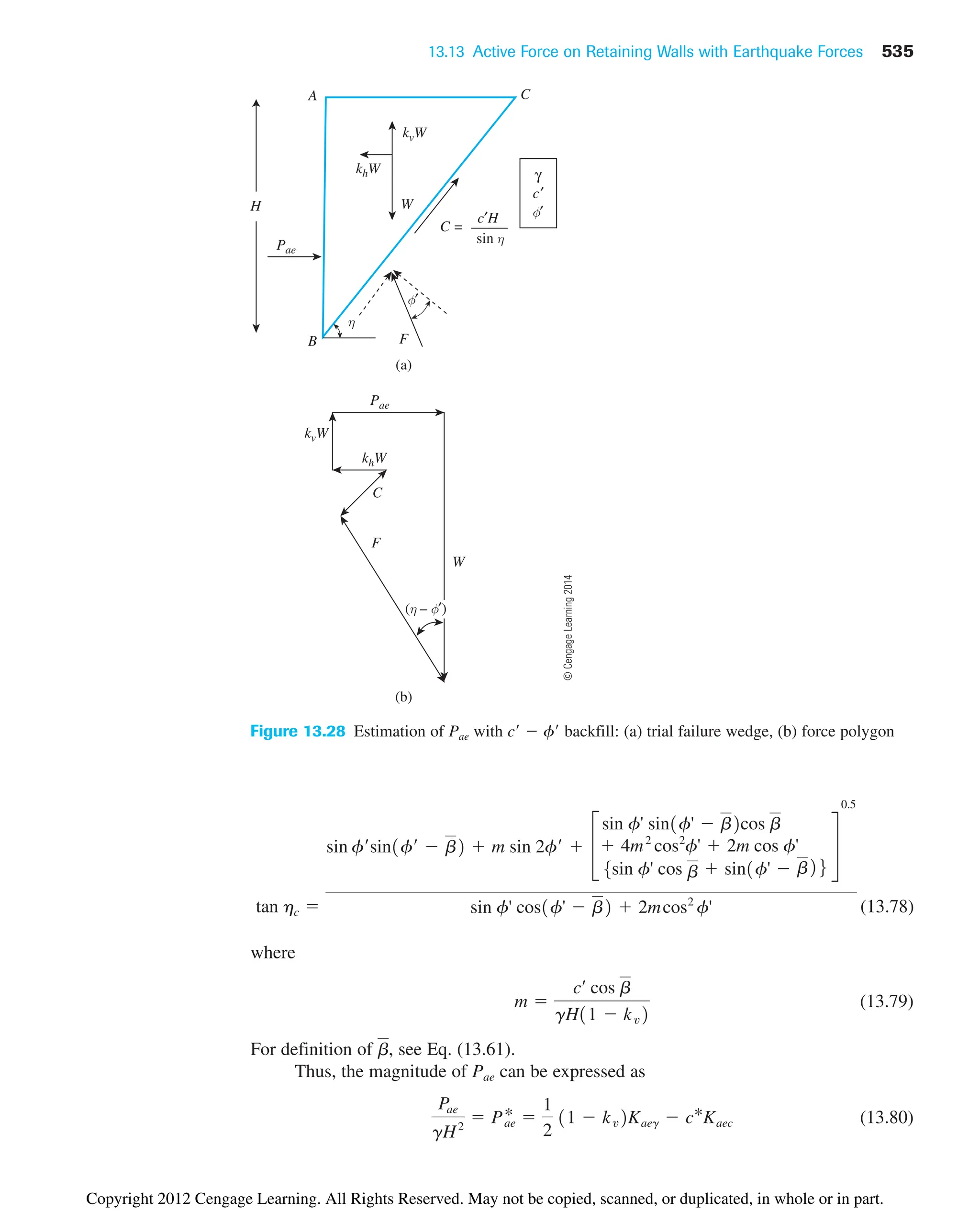
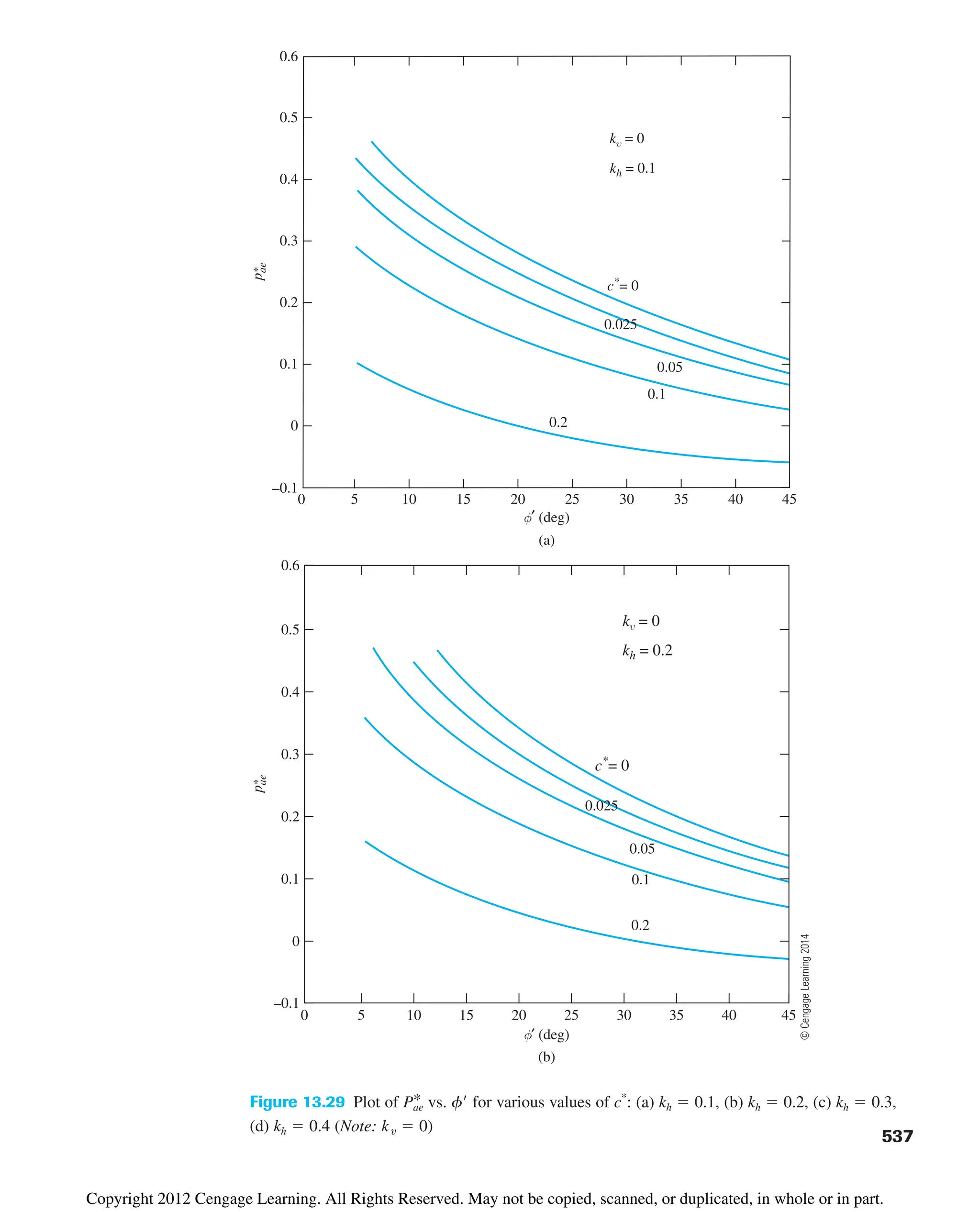
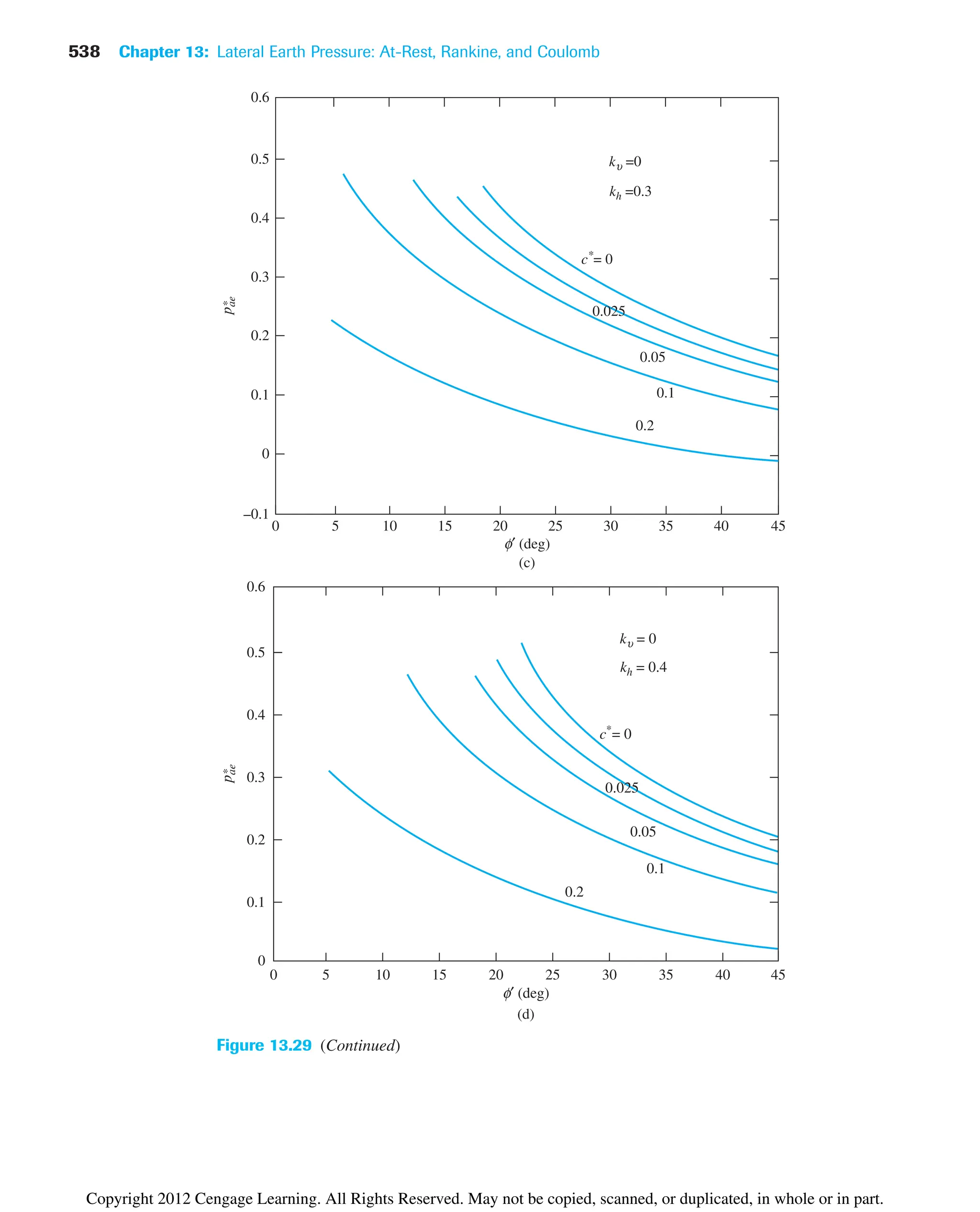
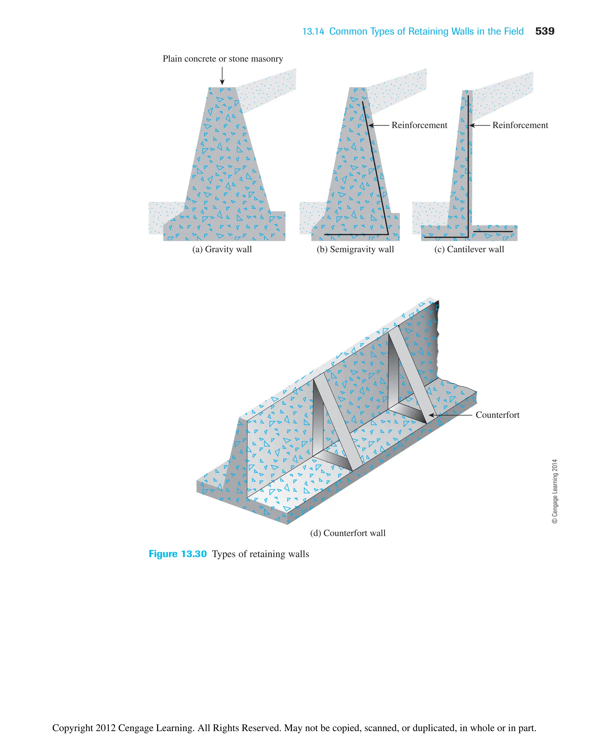
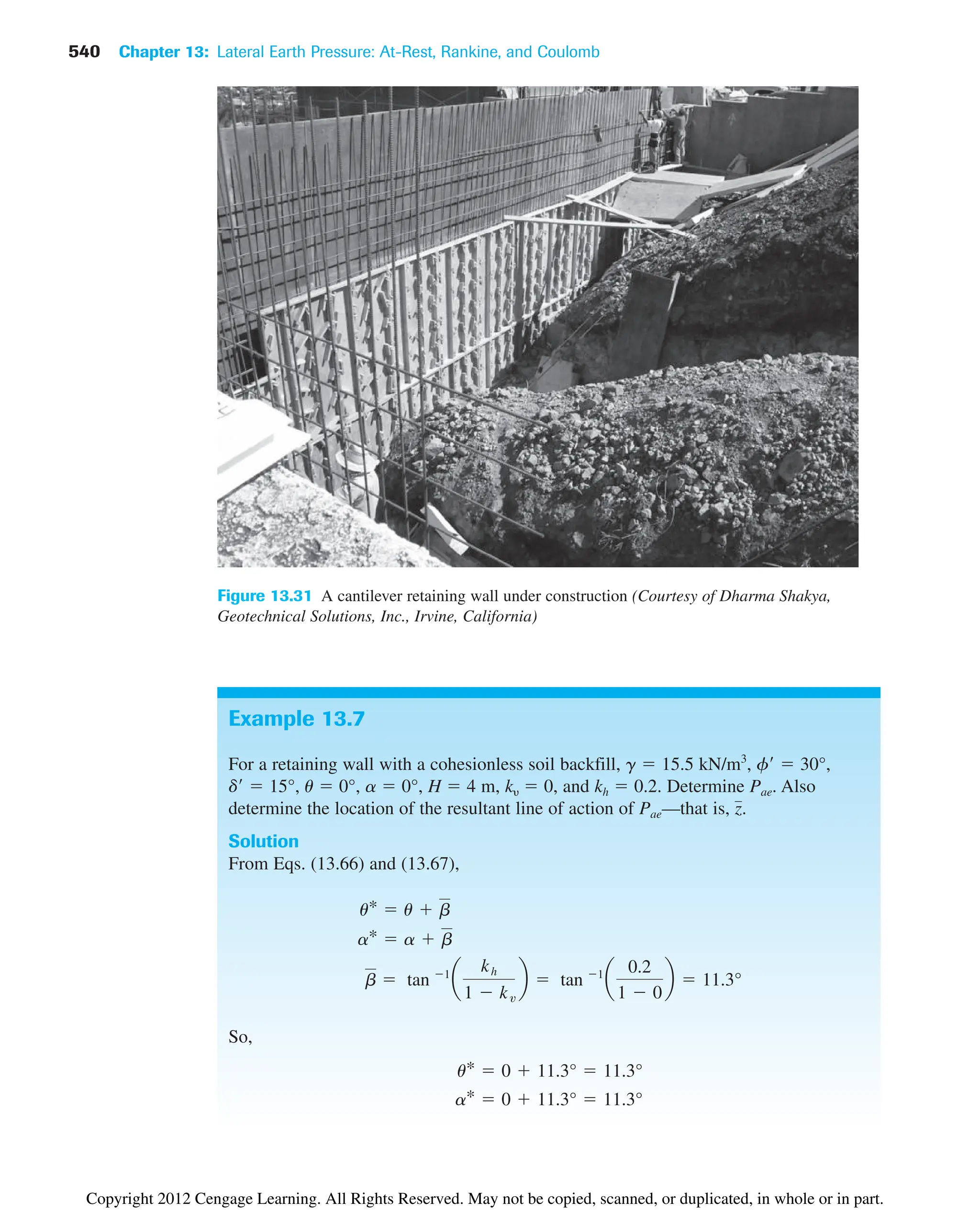
![13.14 Common Types of Retaining Walls in the Field 541
Example 13.8
For a retaining wall with a vertical backfill, the following are given.
• H 8.54 m • g 18.55 kN/m3
• f 20° • kh 0.1
• c 7.9 kN/m2
Determine the magnitude of the active force, Pae.
Solution
From Eq. (13.81),
f œ
20°
c*
cœ
gH
7.9
118.55218.542
0.0499 ⬇ 0.05
From Eq. (13.70),
where Ka is a function of u*
and a*
.
Since d/f 15/30 0.5, we will use Table 13.6. For u*
a*
11.3°, the value
of . Thus,
[Note: We can also get the same values of Pae using Eq. (13.60) and from Table 13.8.]
We now locate the resultant line of action. From Eq. (13.53),
For f 30° and d 15°, Ka 0.3014 (Table 13.6), so
Hence, DPae 56.05 37.37 18.68 kN/m. From Eq. (13.77)
z
Pa a
H
3
b ¢Pae10.6H2
Pae
137.372a
4
3
b 118.68212.42
56.05
1.69 m
Pa 1
210.30142115.521422
37.37 KN/m
Pa 1
2KagH2
Kae
œ
Pae 1
2115.521422
10.452211 02c
cos 2
10 11.32
1 cos 021 cos 2
11.32
d 56.05 kN/m
Ka ⬇ 0.452
Pa1u*, a*2 1
2gH2
Ka
3Pa1u*, a*2411 kv2c
cos 2
1u b2
cos u cos 2
b
d
Pae 3Pa1u*, a*2411 kv2a
cos 2
u*
cos 2
u cos 2
b
b
Copyright 2012 Cengage Learning. All Rights Reserved. May not be copied, scanned, or duplicated, in whole or in part.](https://image.slidesharecdn.com/principlesofgeotechnicalengineering-8thedition-231222125509-7e44d9bf/75/Principles-of-Geotechnical-Engineering-8th-Edition-pdf-561-2048.jpg)
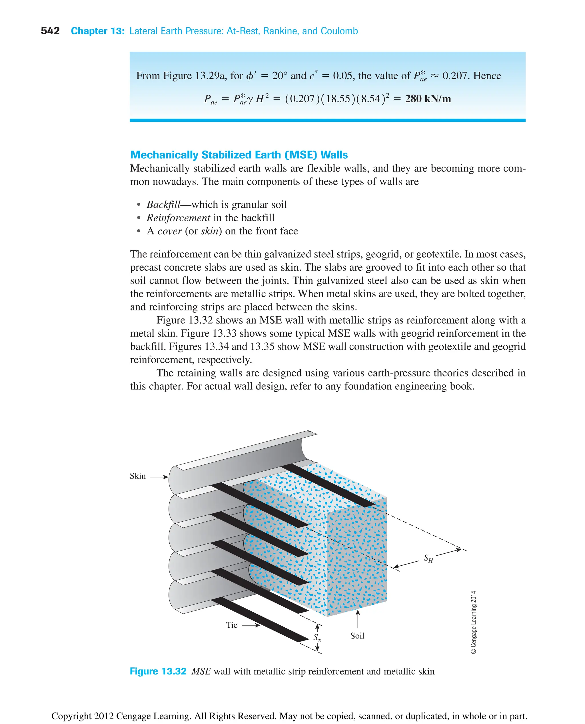
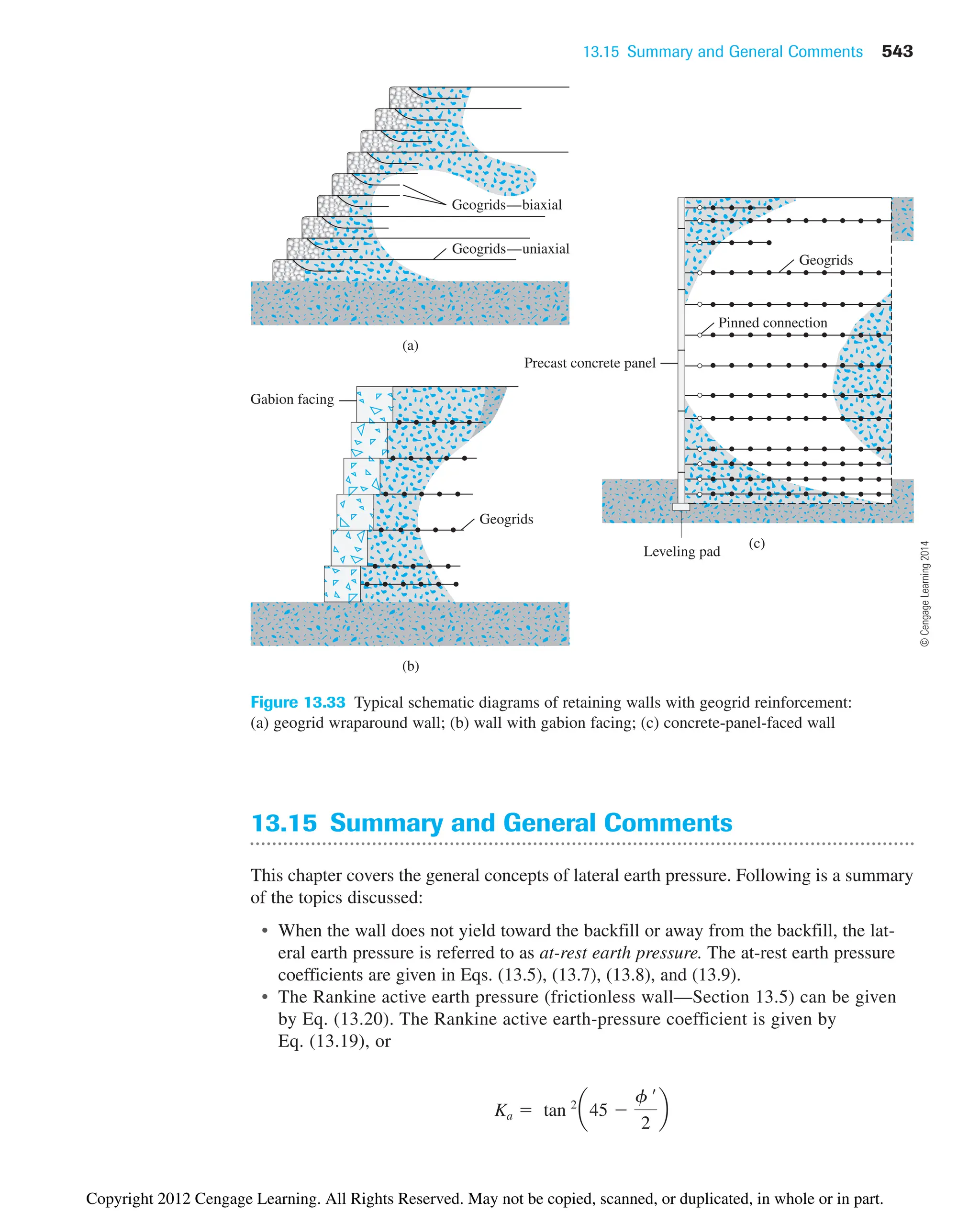
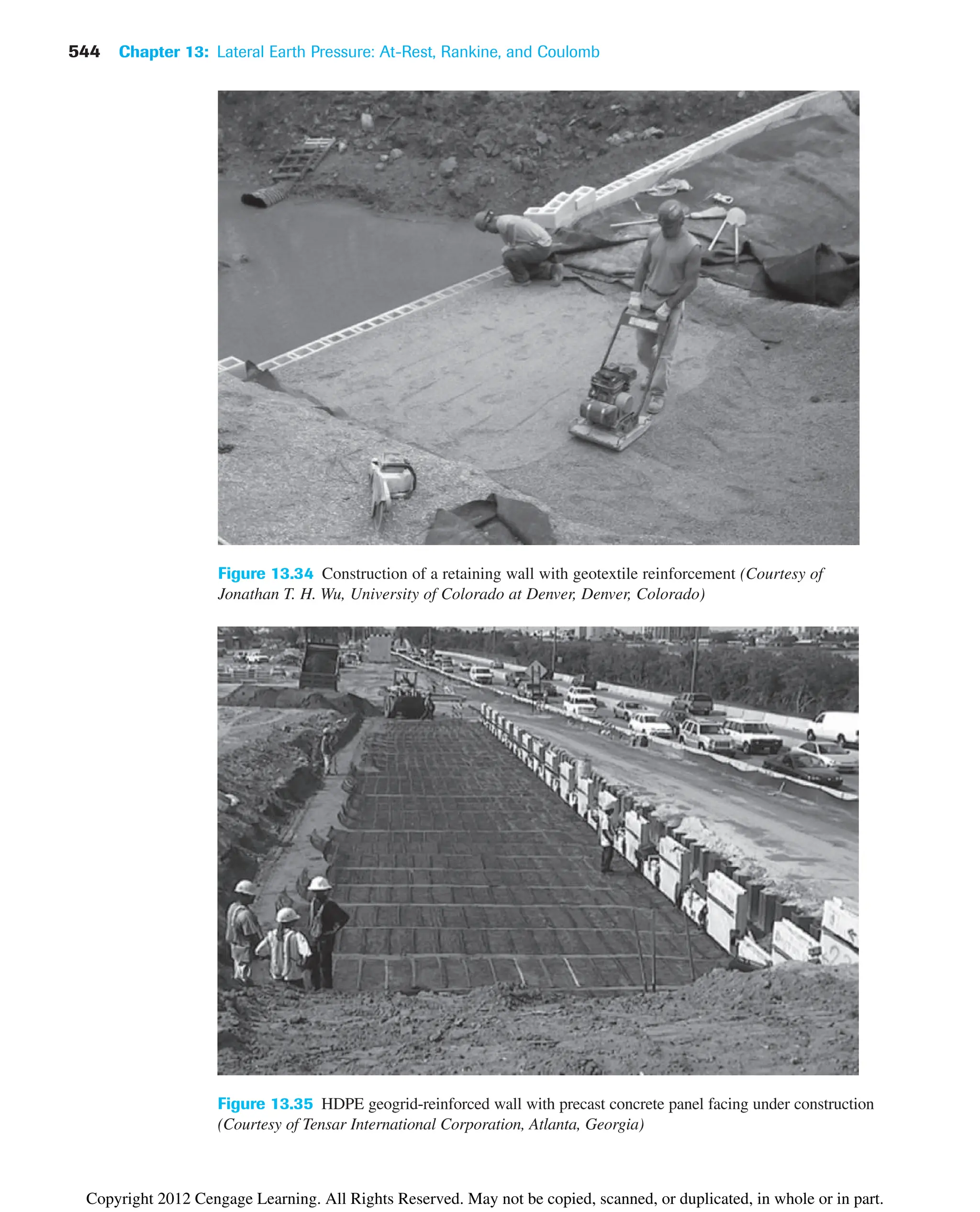
![Problems 545
Problems
13.1 through 13.4 Figure 13.36 shows a retaining wall that is restrained from yielding.
For each problem, determine the magnitude of the lateral earth force per unit
length of the wall. Also, find the location of the resultant, measured from the
bottom of the wall.
z
,
Overconsolidation
Problem H F (deg) G ratio, OCR
13.1 5 m 35 18.1 kN/m3
2
13.2 5.2 m 33 14.9 kN/m3
1.8
13.3 6 m 29 19 kN/m3
1
13.4 5.5 m 40 18 kN/m3
1.5
Sand
Unit weight g (or density r)
f
c 0
d (angle of wall friction) 0
H
Figure 13.36
• The Rankine passive earth-pressure (frictionless wall—Section 13.6) can be given by
Eq. (13.21). The Rankine passive earth-pressure coefficient [Eq. (13.22)] is
• The lateral earth pressure with wall friction and granular backfill can be obtained
from Coulomb’s analysis. Coulomb’s active and passive earth pressure coefficients
are given in Eqs. (13.54) and (13.56), respectively.
• The analysis of active earth pressure with granular and c–f soil backfill
subjected to earthquake forces was discussed in Section 13.13. The active earth
pressure coefficient with granular backfill is given in Eq. (13.60). Similarly,
for a c–f soil backfill, the lateral earth pressure coefficients can be given by
Eqs. (13.82) and (13.83).
Kp tan 2
a45
f œ
2
b
©
Cengage
Learning
2014
©
Cengage
Learning
2014
Copyright 2012 Cengage Learning. All Rights Reserved. May not be copied, scanned, or duplicated, in whole or in part.](https://image.slidesharecdn.com/principlesofgeotechnicalengineering-8thedition-231222125509-7e44d9bf/75/Principles-of-Geotechnical-Engineering-8th-Edition-pdf-565-2048.jpg)
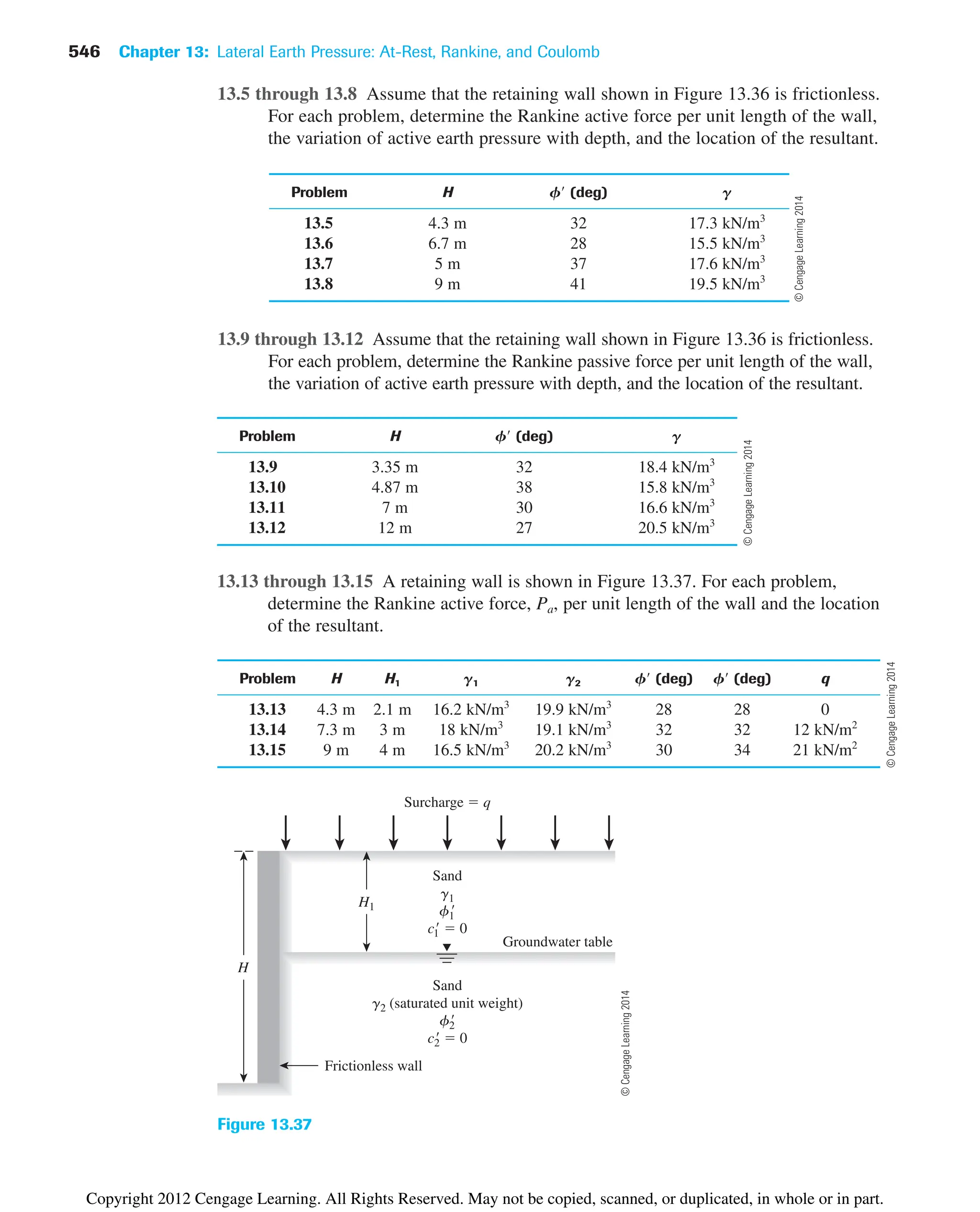
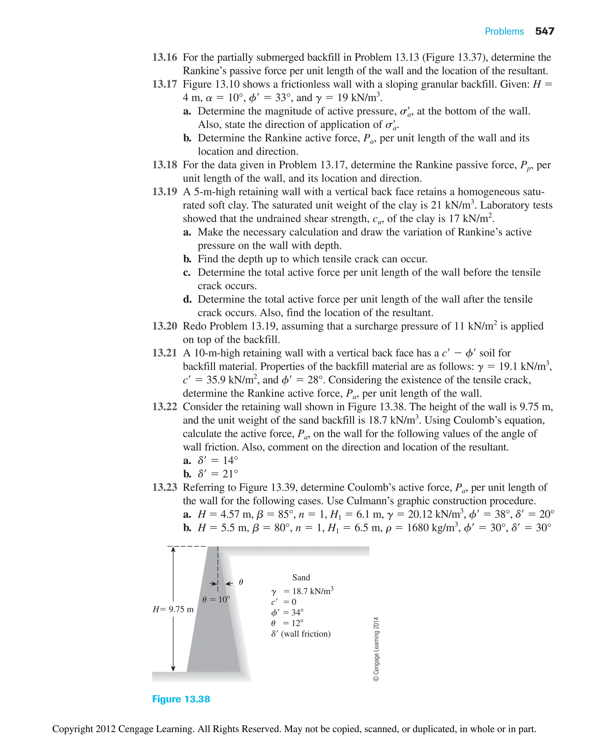
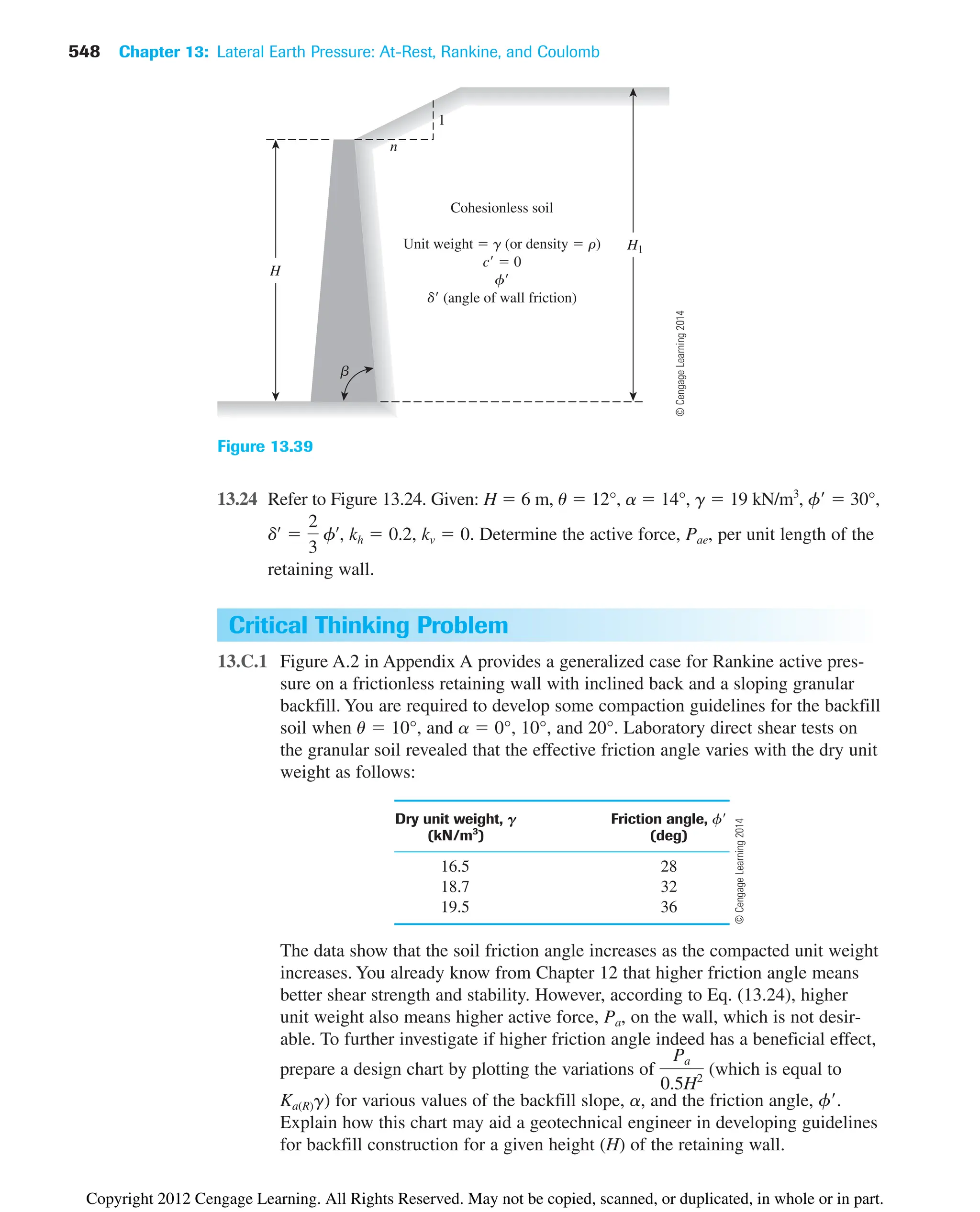
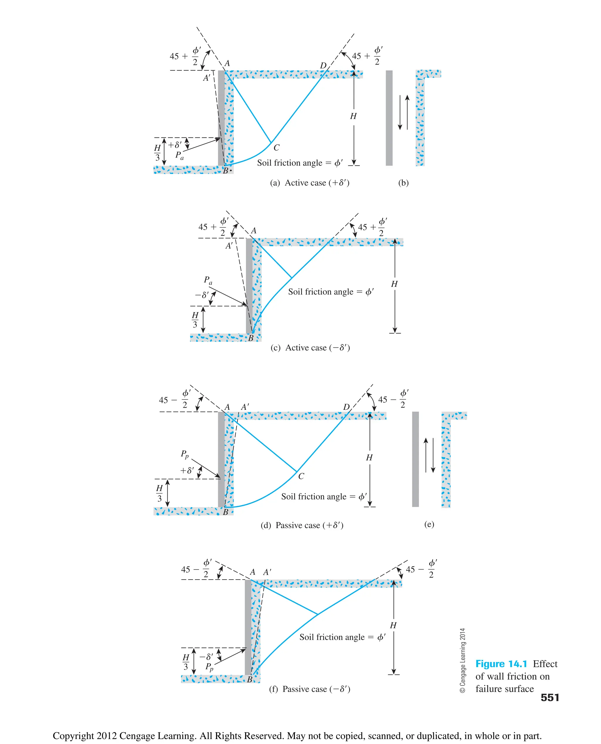
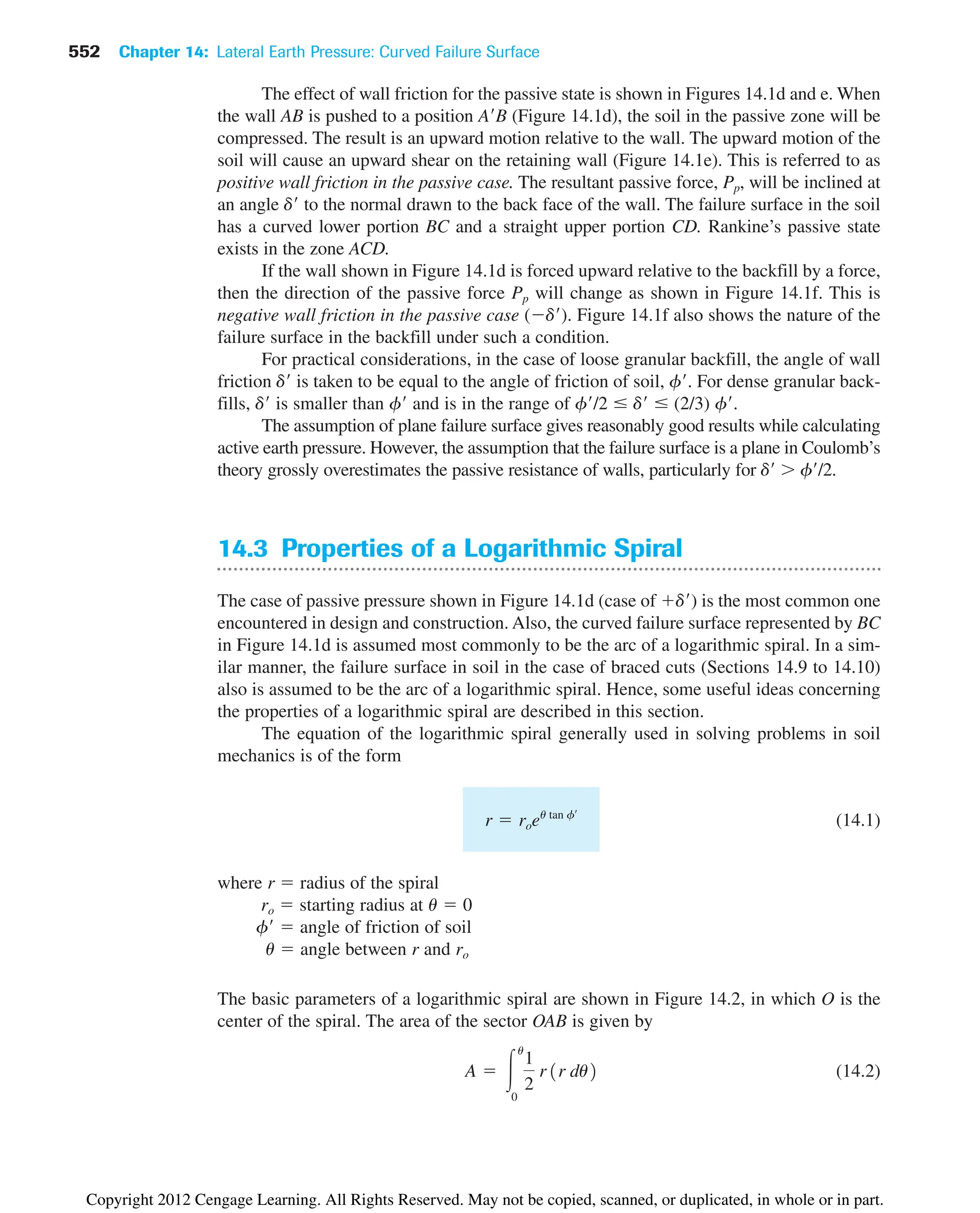
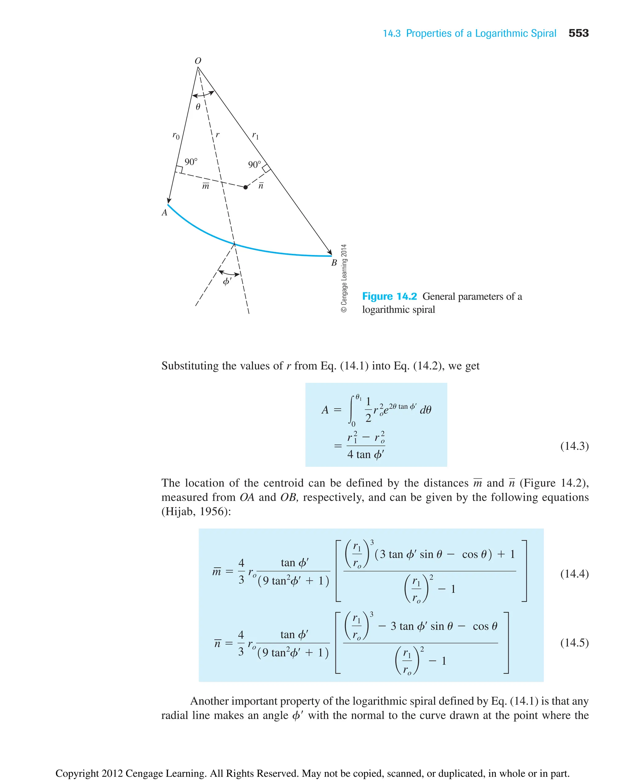
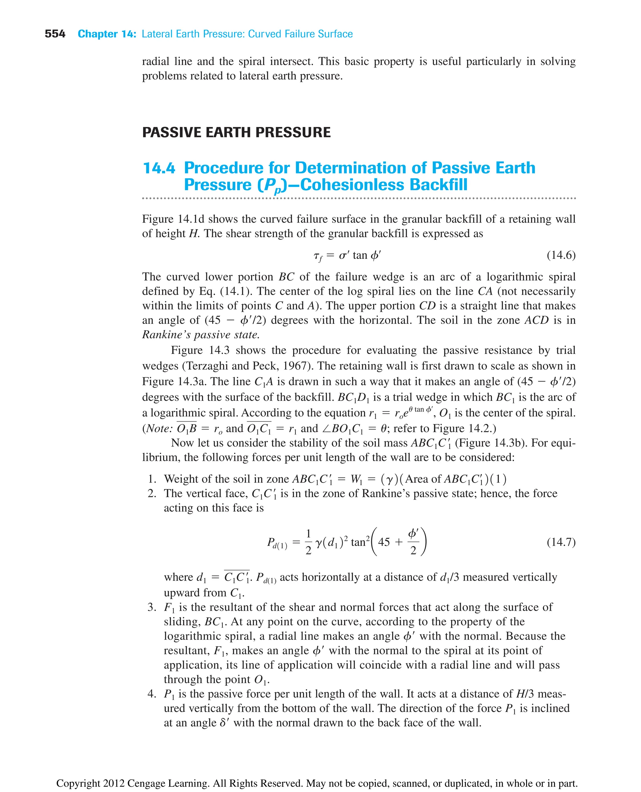
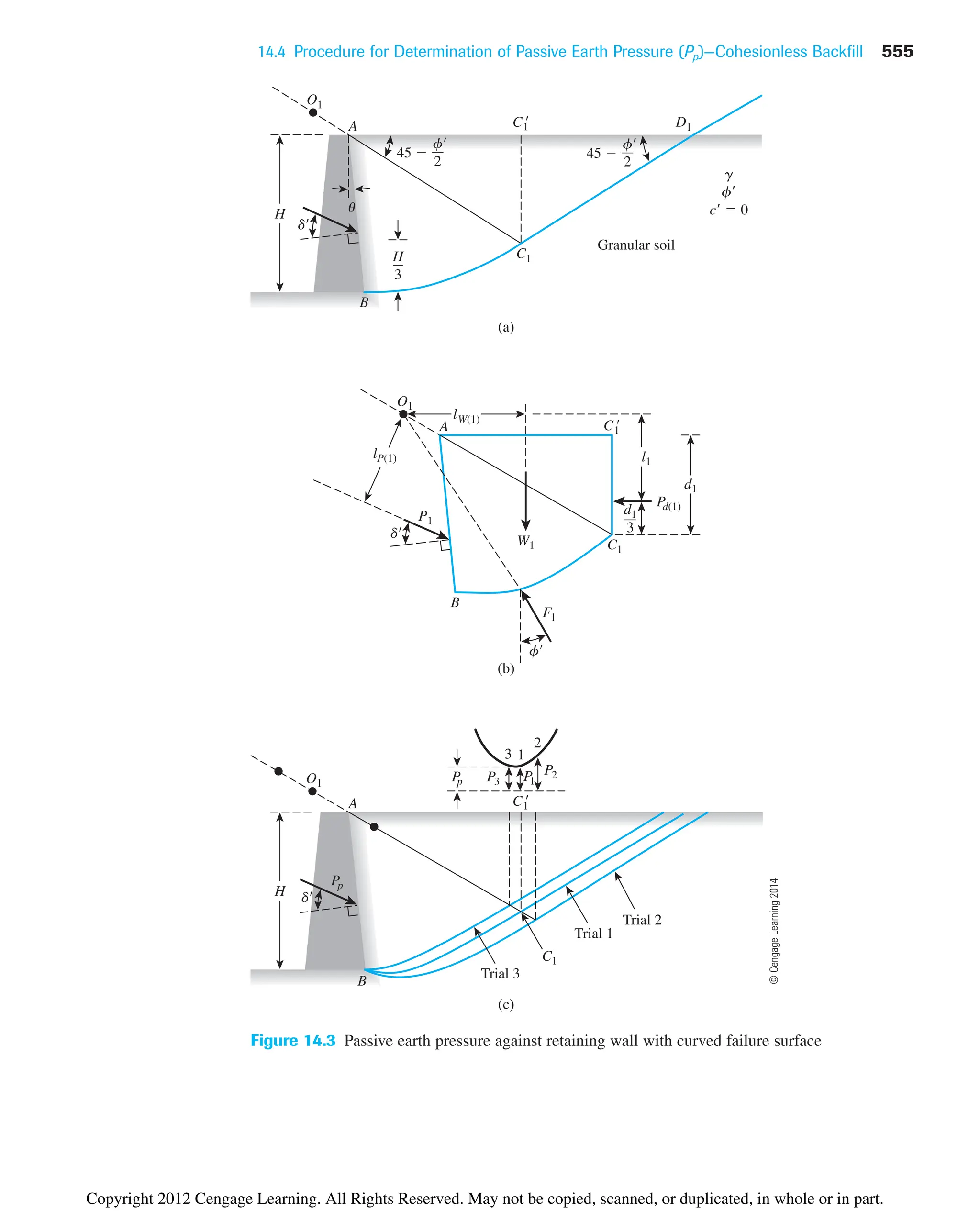
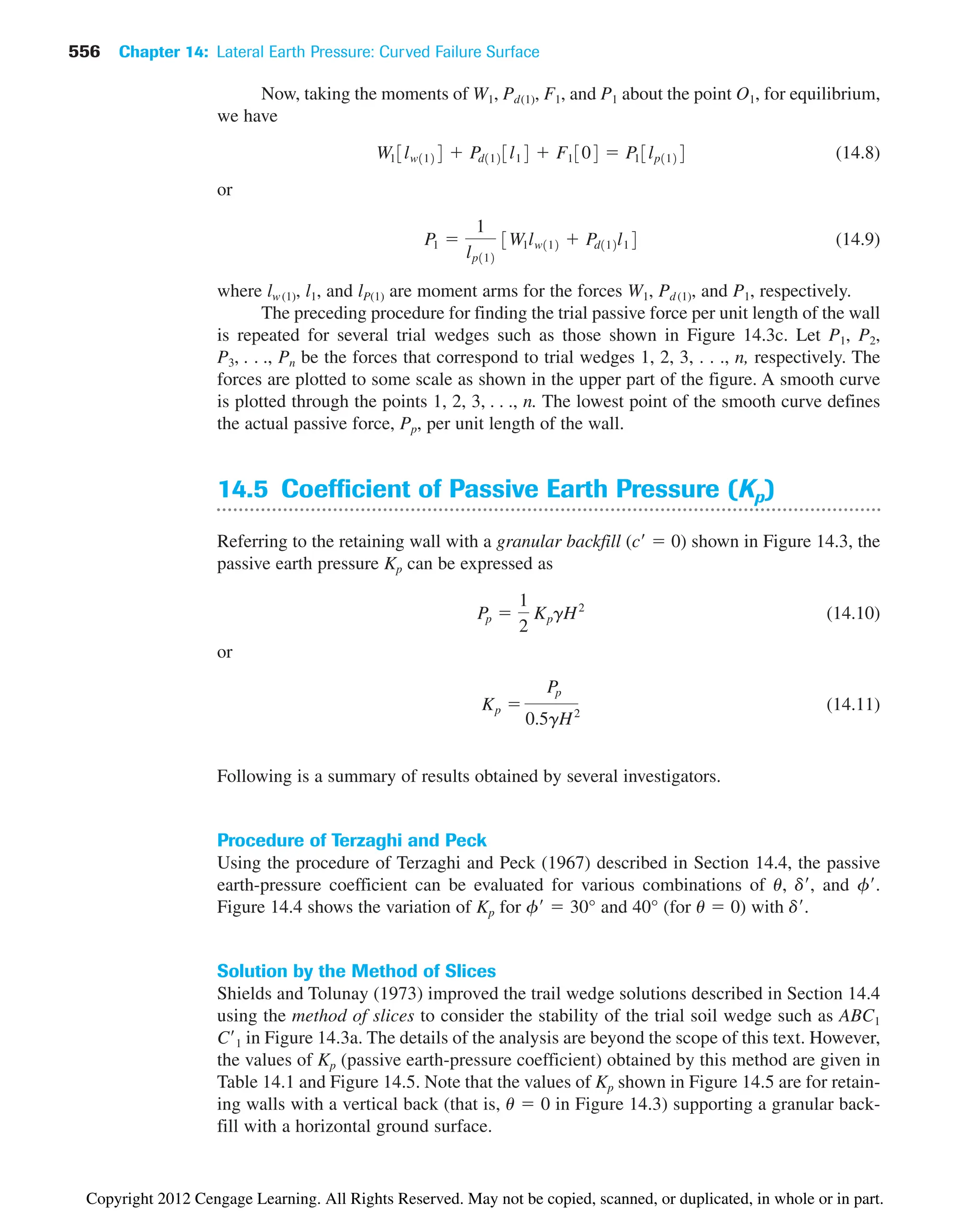
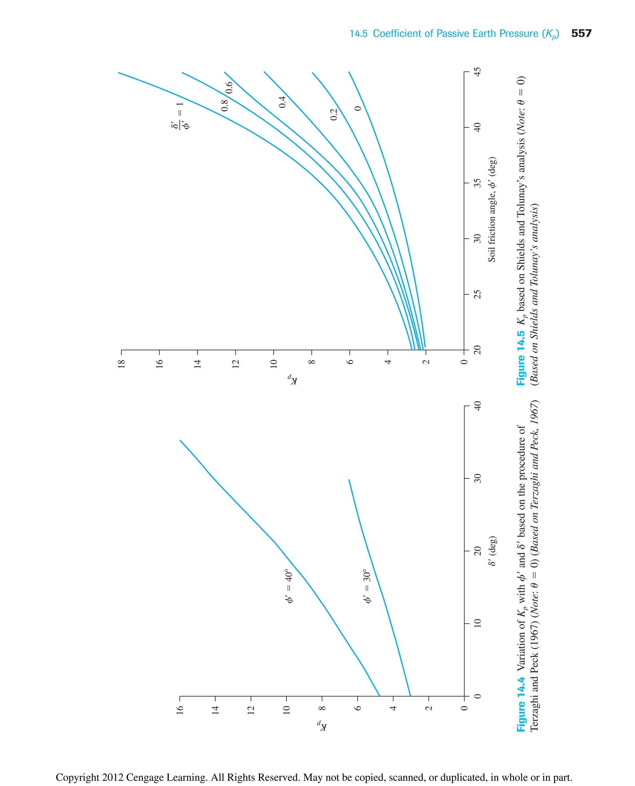
![Table 14.1 Shields and Tolunay’s Values of Kp Based on the Method of Slices
d9 (deg)
f9 (deg) 0 5 10 15 20 25 30 35 40 45
20 2.04 2.26 2.43 2.55 2.70
25 2.46 2.77 3.03 3.23 3.39 3.63
30 3.00 3.43 3.80 4.13 4.40 4.64 5.03
35 3.69 4.29 4.84 5.34 5.80 6.21 6.59 7.25
40 4.69 5.44 6.26 7.05 7.80 8.51 9.18 9.83 11.03
45 5.83 7.06 8.30 9.55 10.80 12.04 13.26 14.46 15.60 18.01
Solution by the Method of Triangular Slices
Zhu and Qian (2000) used the method of triangular slices (such as in the zone of ABC1 in
Figure 14.3a) to obtain the variation of Kp. According to this analysis,
(14.12)
where Kp passive earth pressure coefficient for a given value of u, d, and f
for a given value of u, f, with d 0
R modification factor which is a function of f, u, d/f
The variations of are given in Table 14.2. The interpolated values of R are given
in Table 14.3.
Kp1dœ
02
Kp1dœ
02 Kp
Kp Kp1dœ
02R
558 Chapter 14: Lateral Earth Pressure: Curved Failure Surface
Table 14.2 Variation of [see Eq. (14.12) and Figure 14.3a]*
u (deg)
f9 (deg) 30 25 20 15 10 5 0
20 1.70 1.69 1.72 1.77 1.83 1.92 2.04
21 1.74 1.73 1.76 1.81 1.89 1.99 2.12
22 1.77 1.77 1.80 1.87 1.95 2.06 2.20
23 1.81 1.81 1.85 1.92 2.01 2.13 2.28
24 1.84 1.85 1.90 1.97 2.07 2.21 2.37
25 1.88 1.89 1.95 2.03 2.14 2.28 2.46
26 1.91 1.93 1.99 2.09 2.21 2.36 2.56
27 1.95 1.98 2.05 2.15 2.28 2.45 2.66
28 1.99 2.02 2.10 2.21 2.35 2.54 2.77
29 2.03 2.07 2.15 2.27 2.43 2.63 2.88
30 2.07 2.11 2.21 2.34 2.51 2.73 3.00
31 2.11 2.16 2.27 2.41 2.60 2.83 3.12
32 2.15 2.21 2.33 2.48 2.68 2.93 3.25
33 2.20 2.26 2.39 2.56 2.77 3.04 3.39
34 2.24 2.32 2.45 2.64 2.87 3.16 3.53
35 2.29 2.37 2.52 2.72 2.97 3.28 3.68
Kp1dœ
02
Copyright 2012 Cengage Learning. All Rights Reserved. May not be copied, scanned, or duplicated, in whole or in part.](https://image.slidesharecdn.com/principlesofgeotechnicalengineering-8thedition-231222125509-7e44d9bf/75/Principles-of-Geotechnical-Engineering-8th-Edition-pdf-578-2048.jpg)
![14.5 Coefficient of Passive Earth Pressure (Kp) 559
Table 14.3 Variation of R [Eq. (14.12)]
R for f9 (deg)
u (deg) dⴕ/fⴕ 30 35 40 45
0 0.2 1.2 1.28 1.35 1.45
0.4 1.4 1.6 1.8 2.2
0.6 1.65 1.95 2.4 3.2
0.8 1.95 2.4 3.15 4.45
1.0 2.2 2.85 3.95 6.1
5 0.2 1.2 1.25 1.32 1.4
0.4 1.4 1.6 1.8 2.1
0.6 1.6 1.9 2.35 3.0
0.8 1.9 2.35 3.05 4.3
1.0 2.15 2.8 3.8 5.7
10 0.2 1.15 1.2 1.3 1.4
0.4 1.35 1.5 1.7 2.0
0.6 1.6 1.85 2.25 2.9
0.8 1.8 2.25 2.9 4.0
1.0 2.05 2.65 3.6 5.3
15 0.2 1.15 1.2 1.3 1.35
0.4 1.35 1.5 1.65 1.95
0.6 1.55 1.8 2.2 2.7
0.8 1.8 2.2 2.8 3.8
1.0 2.0 2.6 3.4 4.95
20 0.2 1.15 1.2 1.3 1.35
0.4 1.35 1.45 1.65 1.9
0.6 1.5 1.8 2.1 2.6
0.8 1.8 2.1 2.6 3.55
1.0 1.9 2.4 3.2 4.8
Table 14.2 (continued)
u (deg)
f (deg) 30 25 20 15 10 5 0
36 2.33 2.43 2.59 2.80 3.07 3.41 3.84
37 2.38 2.49 2.66 2.89 3.18 3.55 4.01
38 2.43 2.55 2.73 2.98 3.29 3.69 4.19
39 2.48 2.61 2.81 3.07 3.41 3.84 4.38
40 2.53 2.67 2.89 3.17 3.53 4.00 4.59
41 2.59 2.74 2.97 3.27 3.66 4.16 4.80
42 2.64 2.80 3.05 3.38 3.80 4.34 5.03
43 2.70 2.88 3.14 3.49 3.94 4.52 5.27
44 2.76 2.94 3.23 3.61 4.09 4.72 5.53
45 2.82 3.02 3.32 3.73 4.25 4.92 5.80
*
Based on Zhu and Qian, 2000
©
Cengage
Learning
2014
Copyright 2012 Cengage Learning. All Rights Reserved. May not be copied, scanned, or duplicated, in whole or in part.](https://image.slidesharecdn.com/principlesofgeotechnicalengineering-8thedition-231222125509-7e44d9bf/75/Principles-of-Geotechnical-Engineering-8th-Edition-pdf-579-2048.jpg)
![560 Chapter 14: Lateral Earth Pressure: Curved Failure Surface
14.6 Caquot and Kerisel Solution for Passive Earth
Pressure (Granular Backfill)
Figure 14.6 shows a retaining wall with an inclined back and a horizontal backfill. For this
case, the passive pressure per unit length of the wall can be calculated as
(14.13)
where Kp the passive pressure coefficient
For definition of H1, refer to Figure 14.6. The variation of Kp determined by
Caquot and Kerisel (1948) also is shown in Figure 14.6. It is important to note that the
Kp values shown are for d/f 1. If d/f ⬆ 1, the following procedure must be used
to determine Kp.
1. Assume d and f.
2. Calculate d/f.
3. Using the ratio of d/f (step 2), determine the reduction factor, R, from Table 14.4.
4. Determine Kp from Figure 14.6 for d/f 1
5. Calculate Kp for the required d/f as
(14.14)
Kp 1Rœ
23Kp1dœ
/fœ
124
Pp
1
2
gH1
2
Kp
0 10 20 30 40 45
2
1
3
4
5
6
7
8
9
10
11
12
13
14
15
− 30º
+ 20°
+ 30°
+ 40°
Pp
H1 + u
Coefficient
of
passive
pressures,
K
p
+ 10°
− 20º
−10º
u = 0º
d'
H1
3
Failure surface
Logarithmic spiral
Soil friction angle, f′ (deg)
45 −
2
45 −
2
s′p = kpgΗ1
f′
d
f′
Figure 14.6 Caquot and Kerisel’s solution for Kp [Eq. (14.13)]
©
Cengage
Learning
2014
Copyright 2012 Cengage Learning. All Rights Reserved. May not be copied, scanned, or duplicated, in whole or in part.](https://image.slidesharecdn.com/principlesofgeotechnicalengineering-8thedition-231222125509-7e44d9bf/75/Principles-of-Geotechnical-Engineering-8th-Edition-pdf-580-2048.jpg)
![14.6 Caquot and Kerisel Solution for Passive Earth Pressure (Granular Backfill) 561
0
1.0
2.0
3.0
4.0
5.0
10.0
K
p
20.0
30.0
40.0
50.0
100.0
10
H
+α
σp = Kpγz
H
3
Log spiral
Pp
20 30
φ′ (deg)
40
−0.9
−0.8
−0.6
−0.4
−0.2
0.0
0.2
0.4
45
0.6
0.8
+1
α/φ′=
δ′
Figure 14.7 Caquot and Kerisel’s solution for Kp [Eq. (14.15)]
©
Cengage
Learning
2014
Copyright 2012 Cengage Learning. All Rights Reserved. May not be copied, scanned, or duplicated, in whole or in part.](https://image.slidesharecdn.com/principlesofgeotechnicalengineering-8thedition-231222125509-7e44d9bf/75/Principles-of-Geotechnical-Engineering-8th-Edition-pdf-581-2048.jpg)
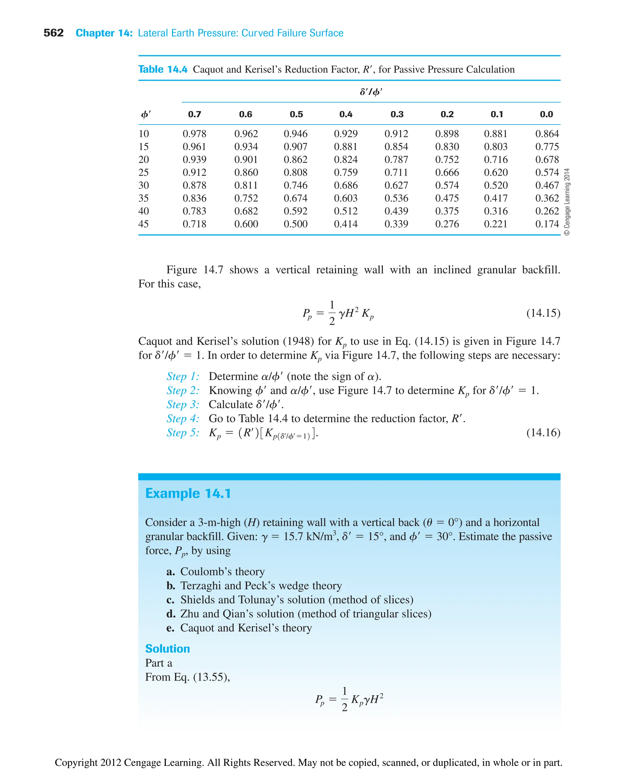
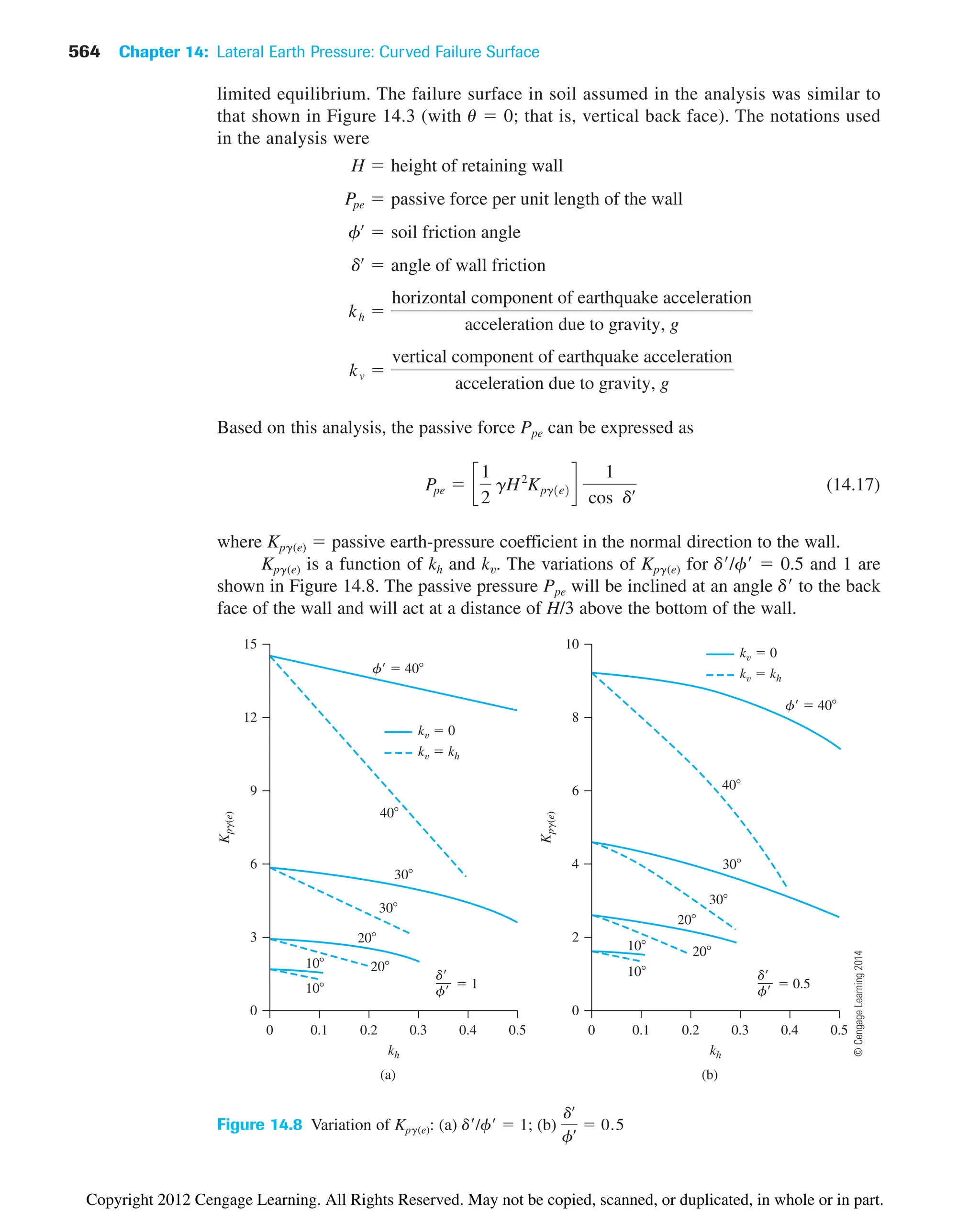
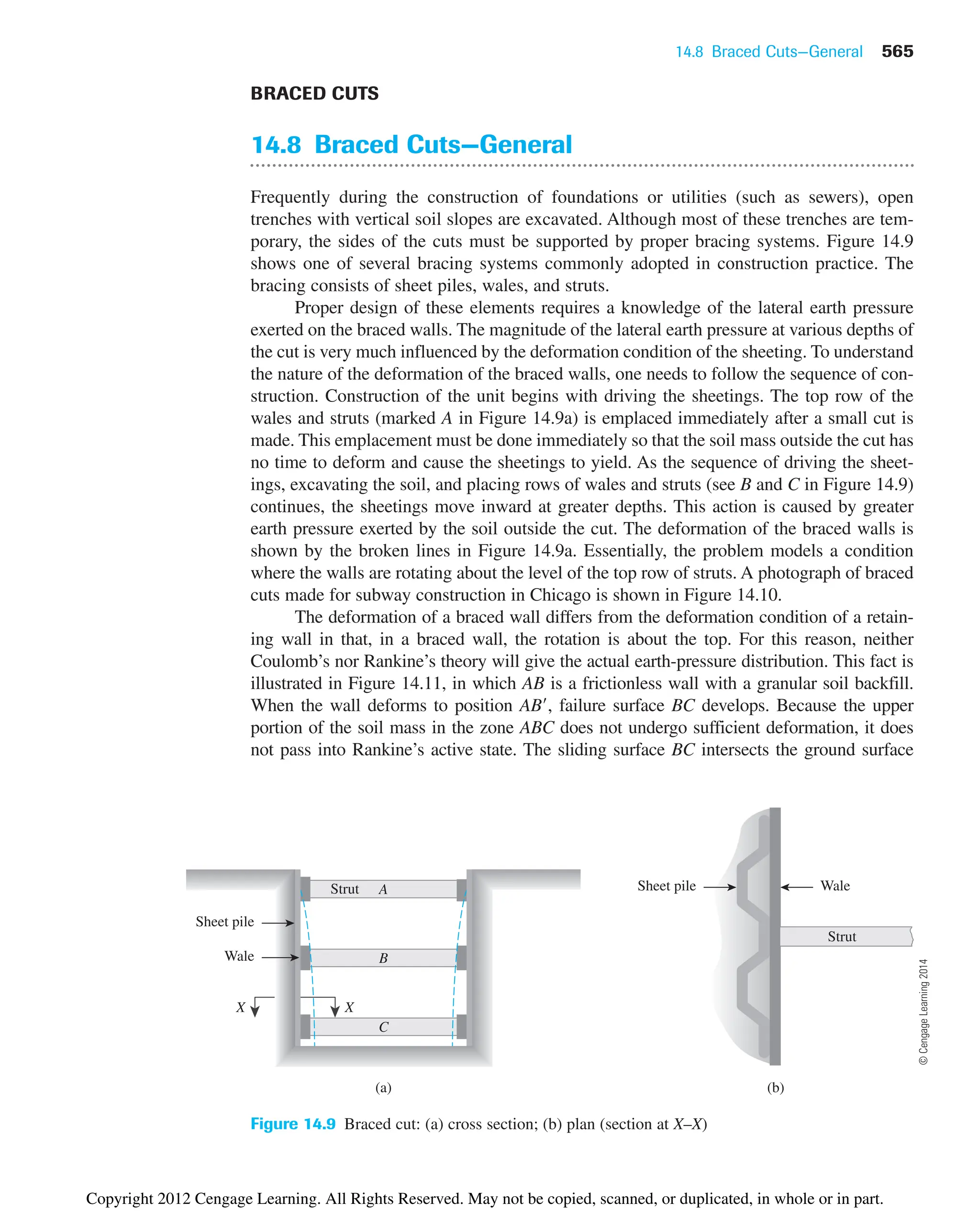
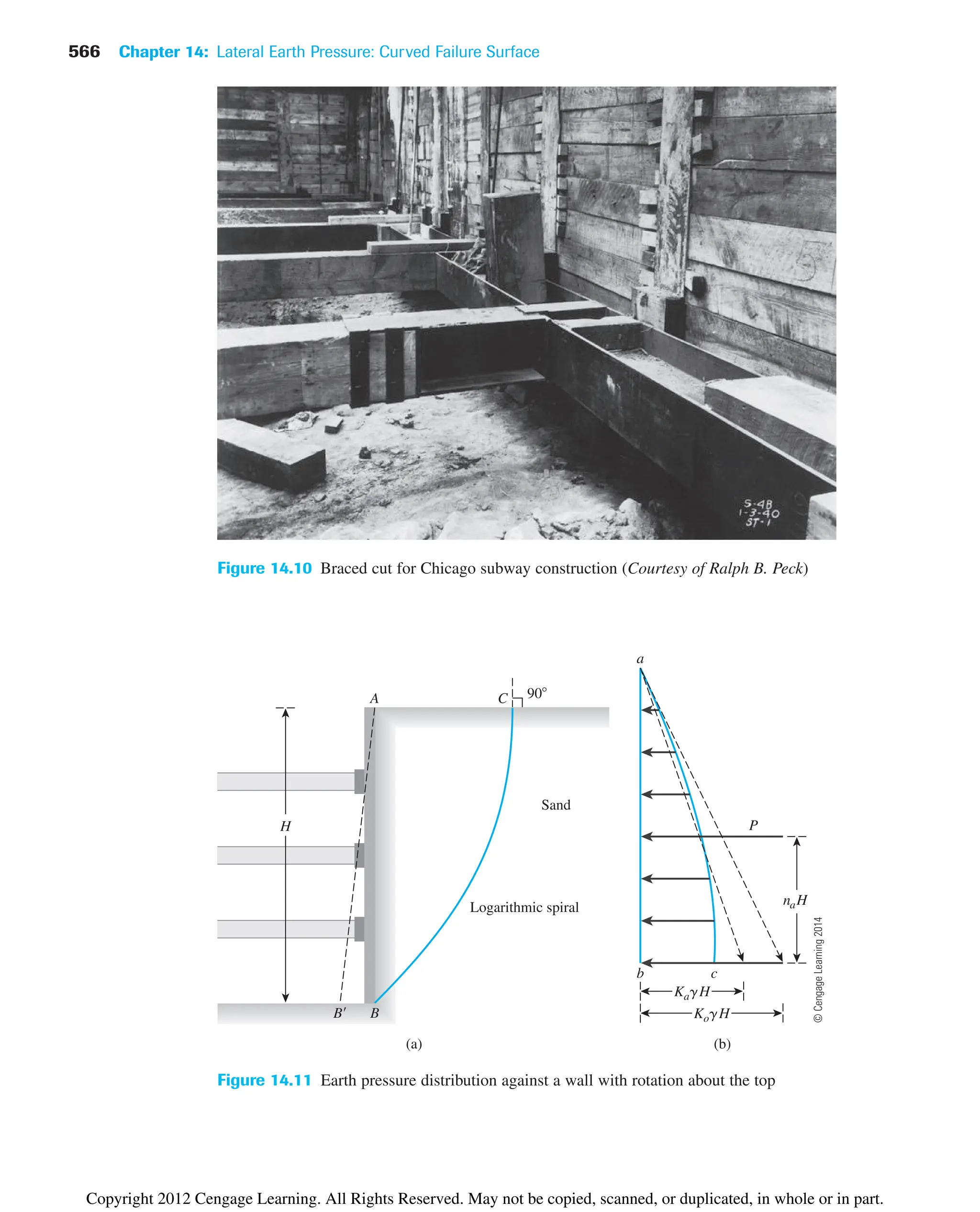
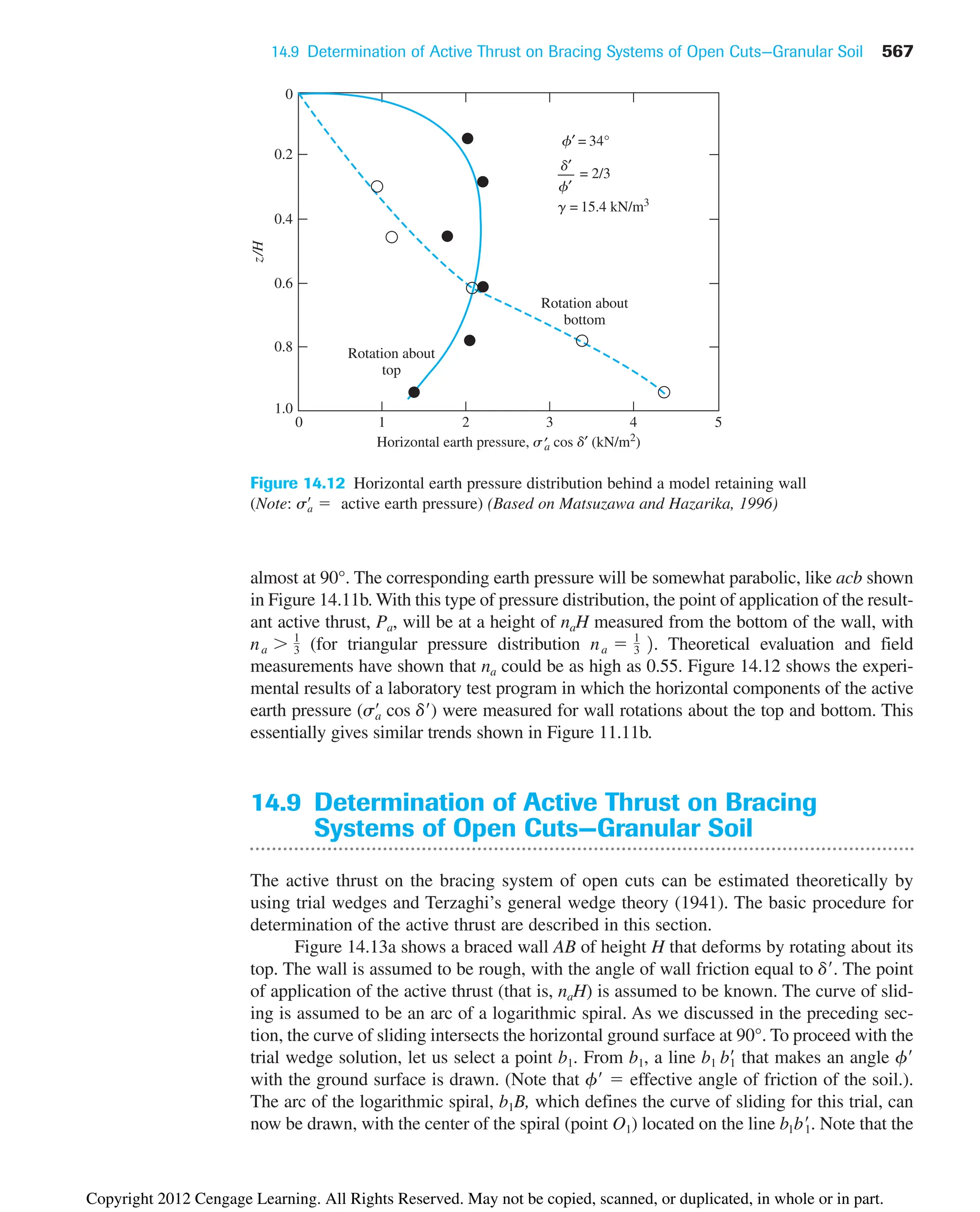
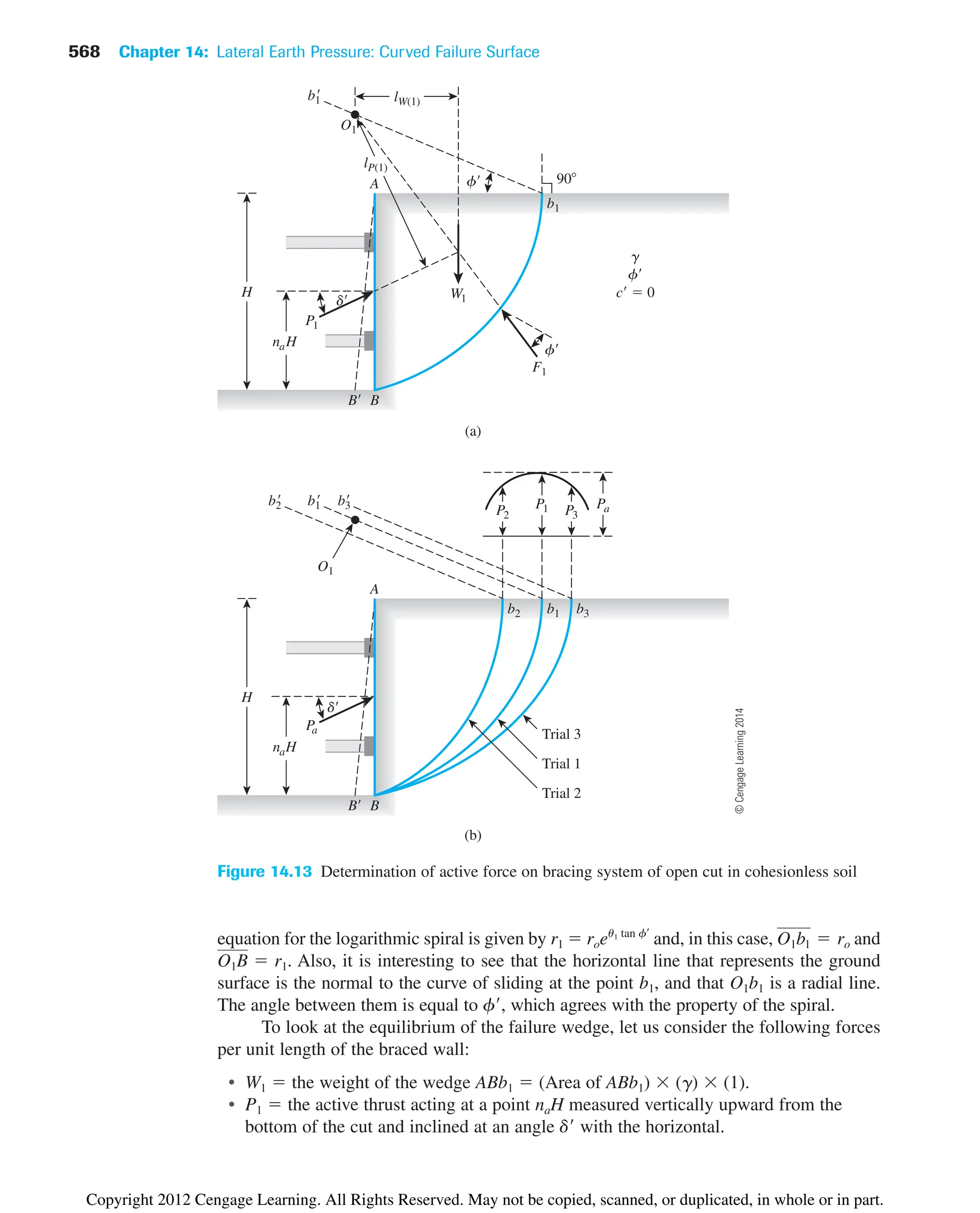
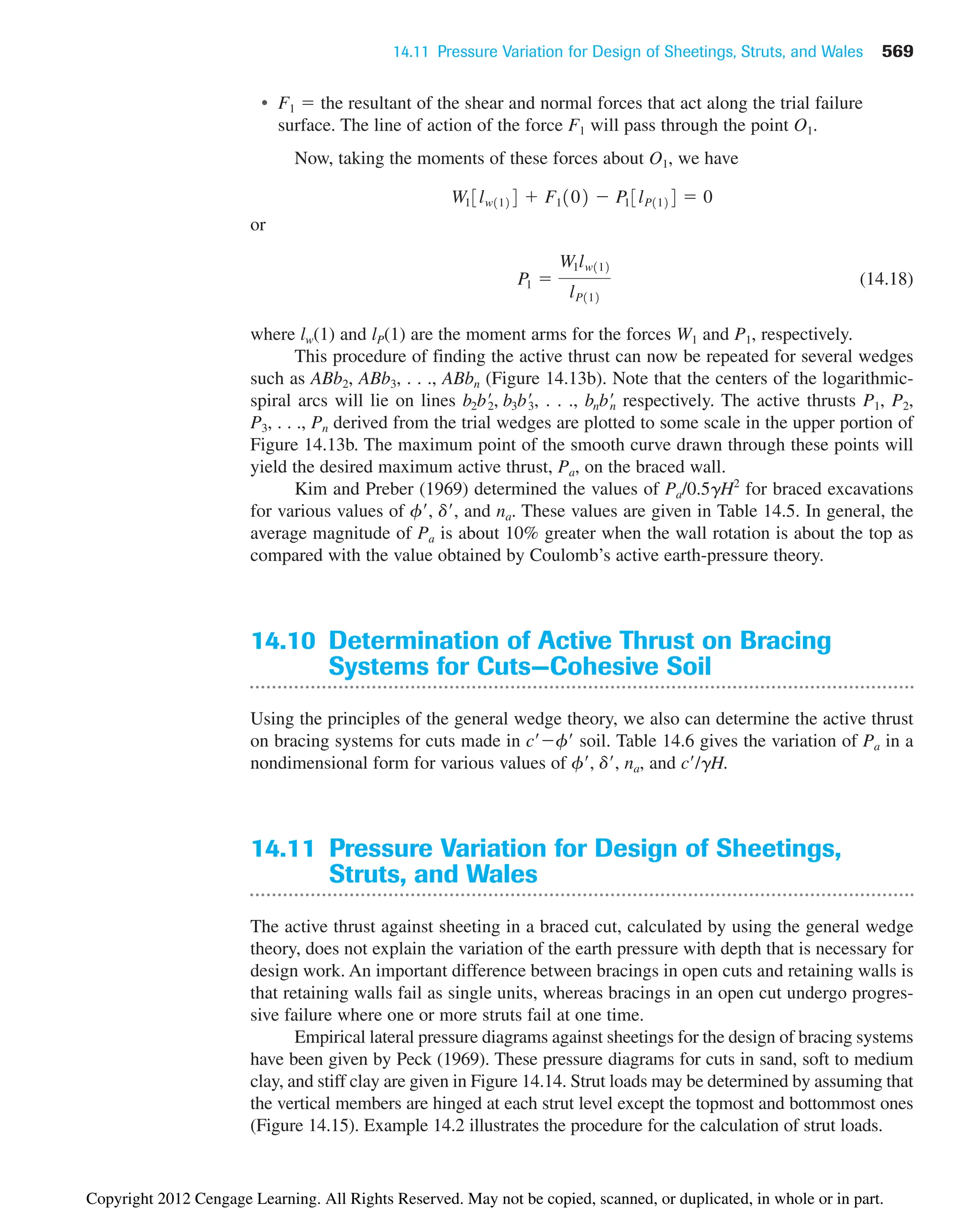
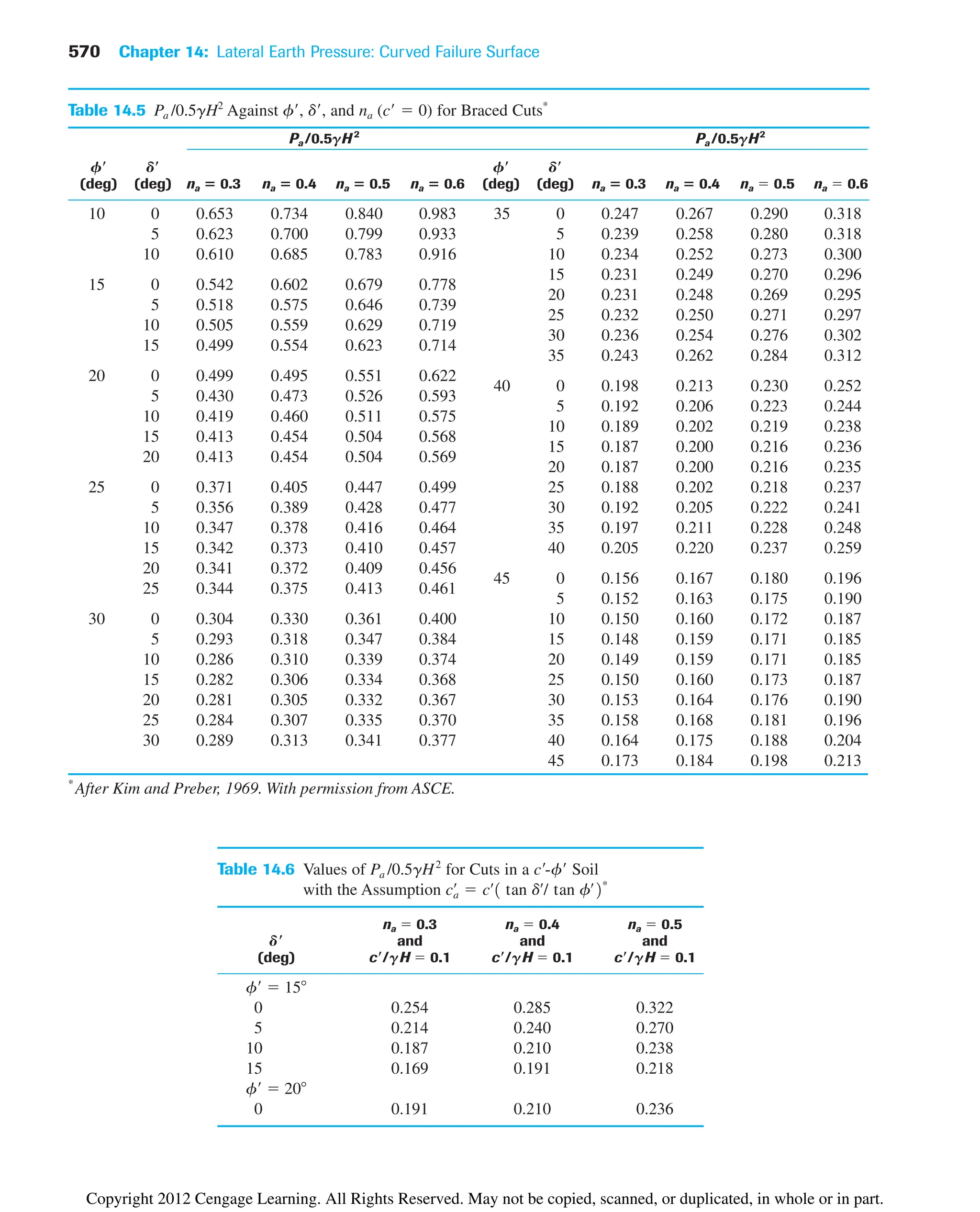
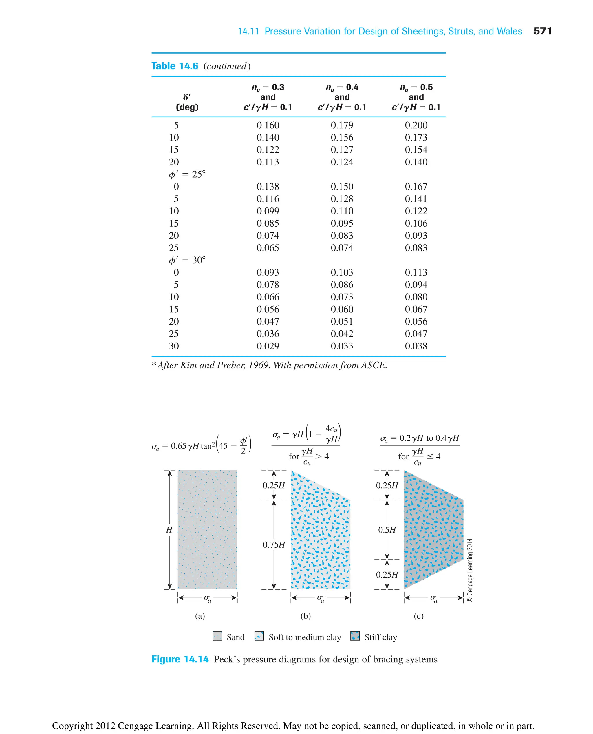
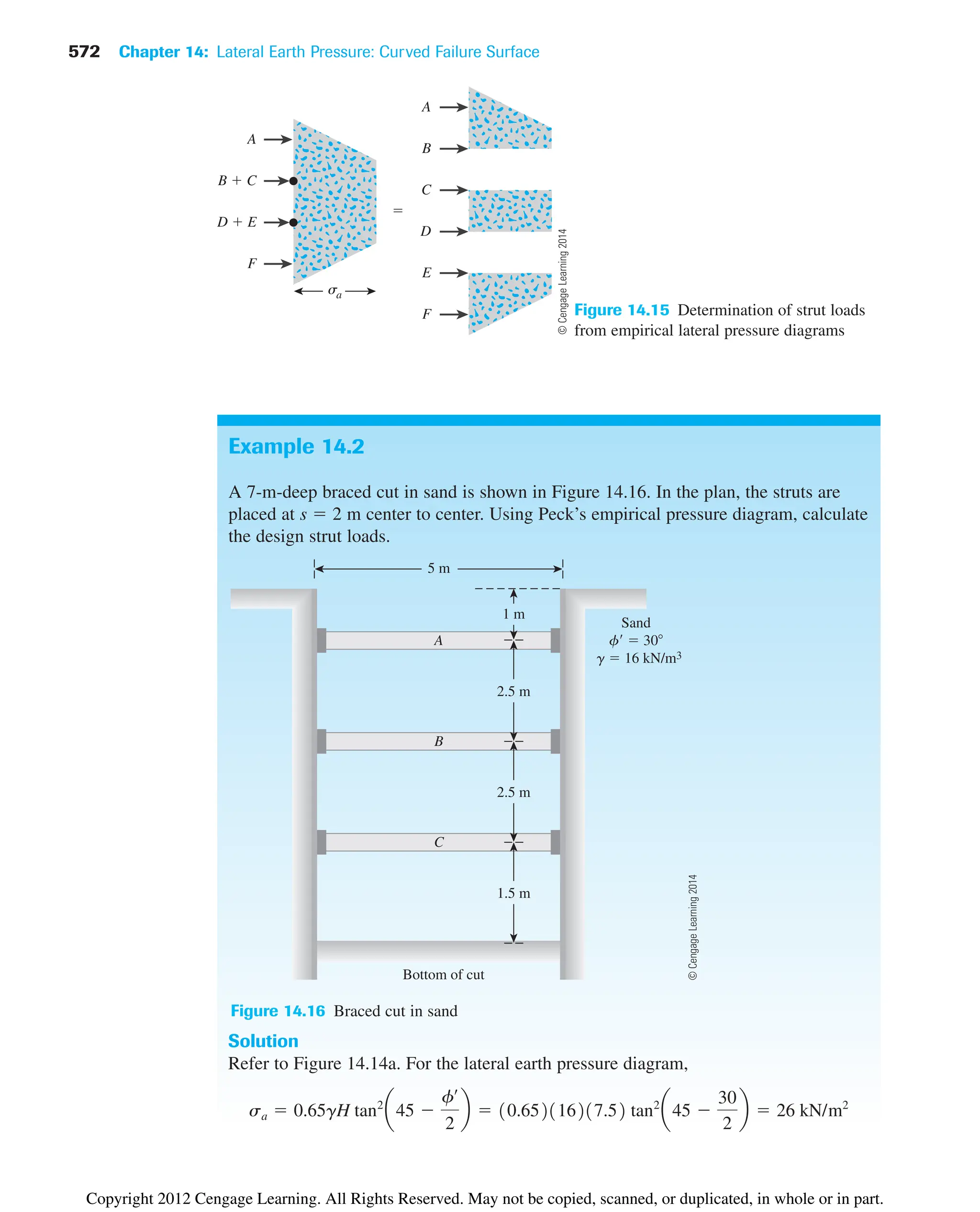
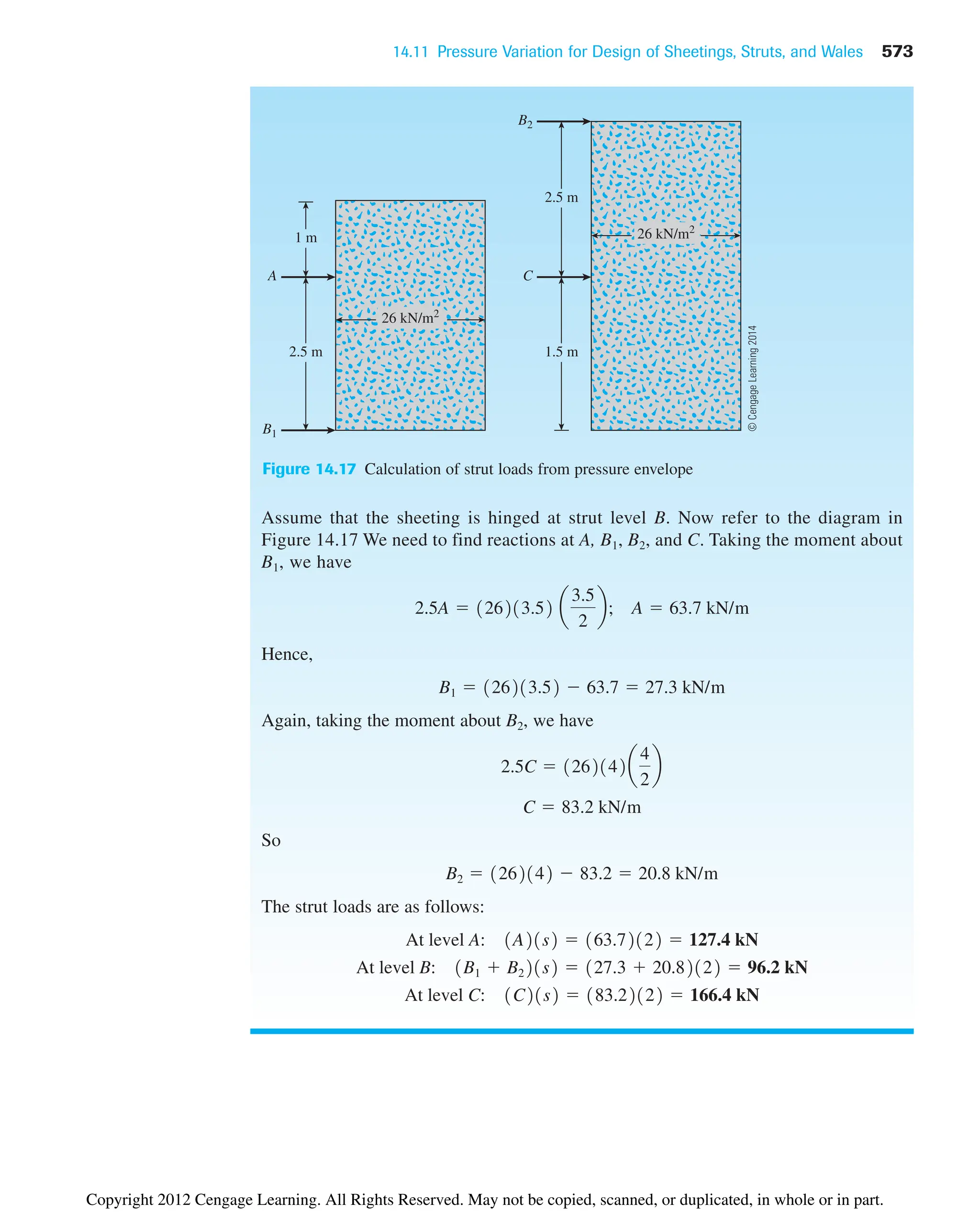
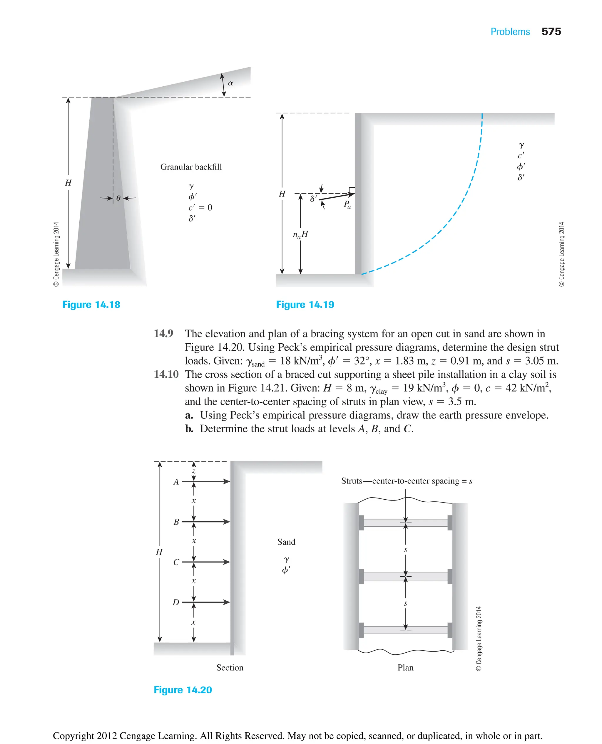
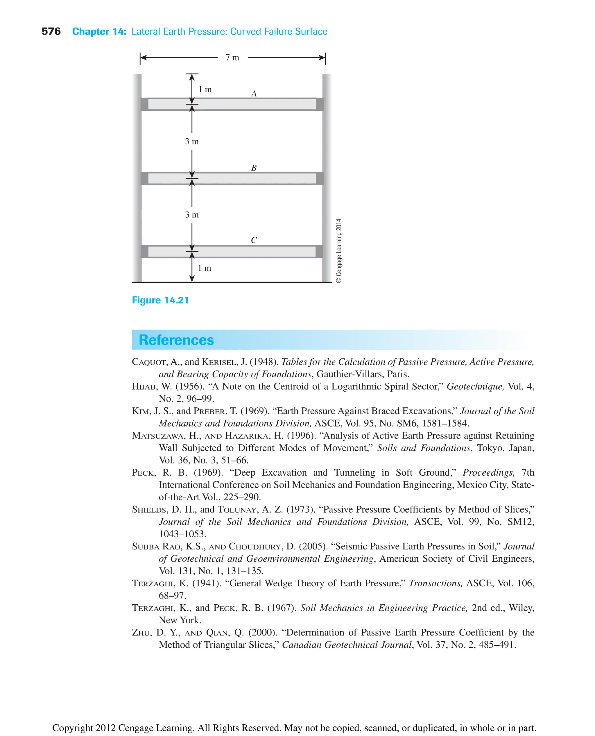
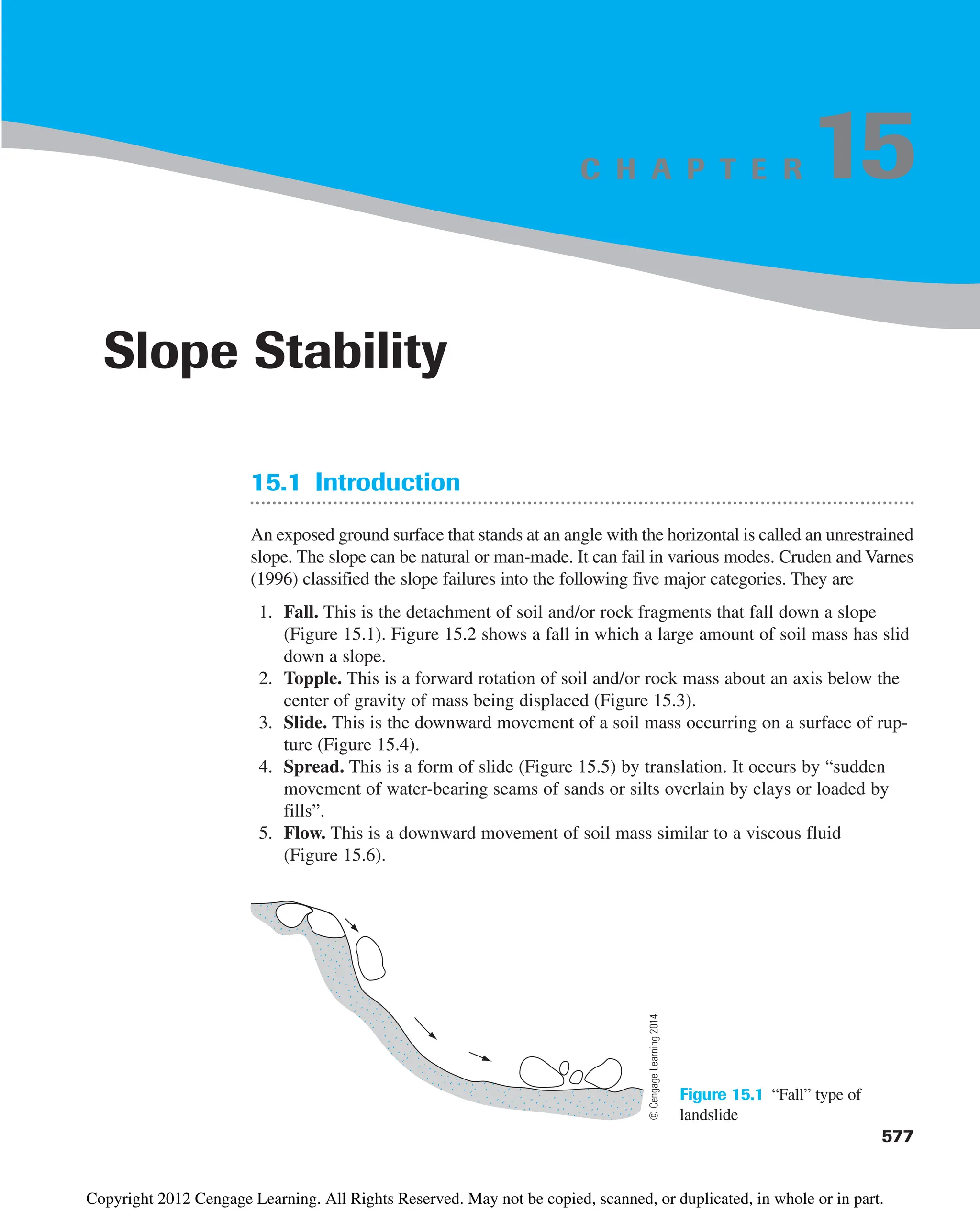
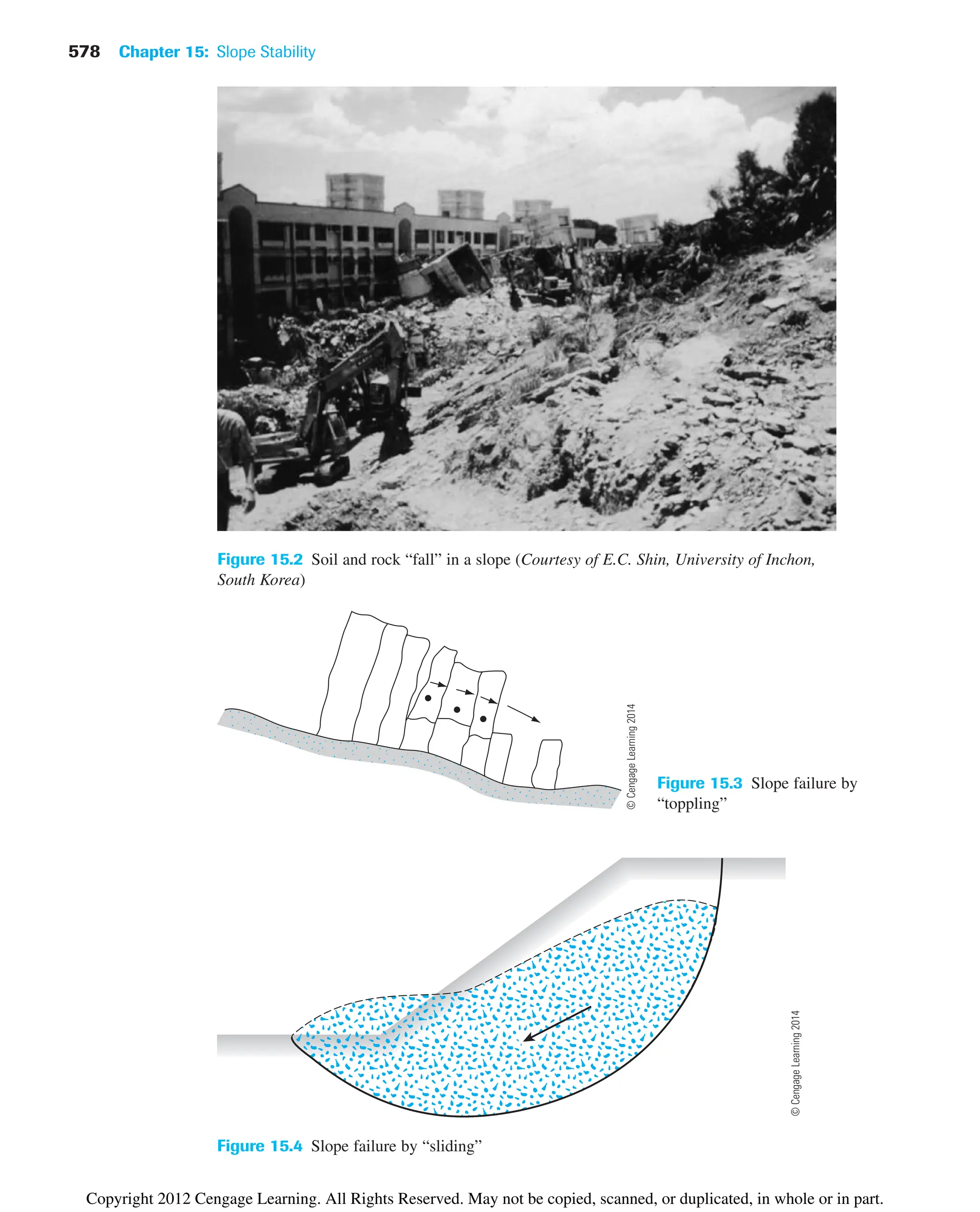
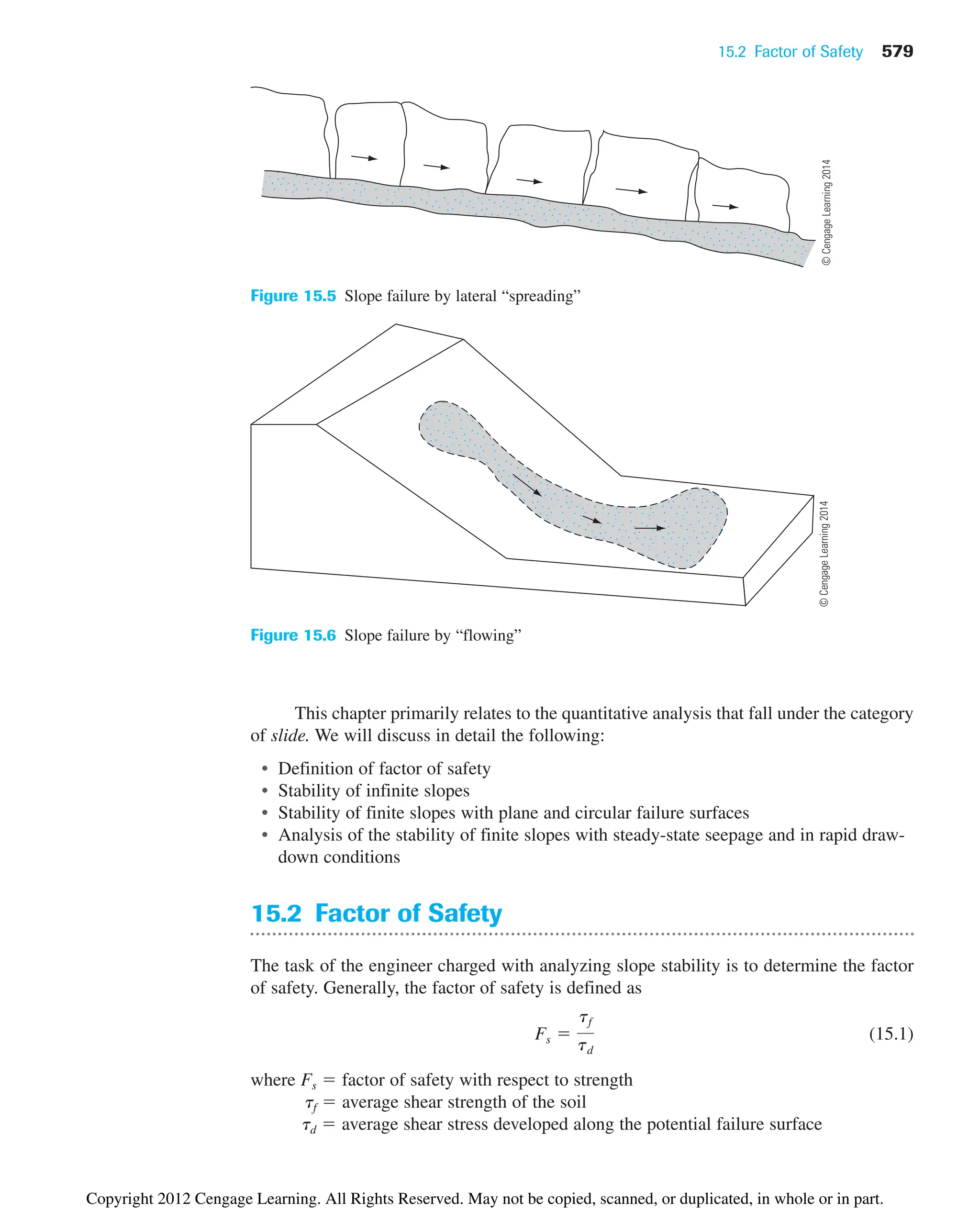
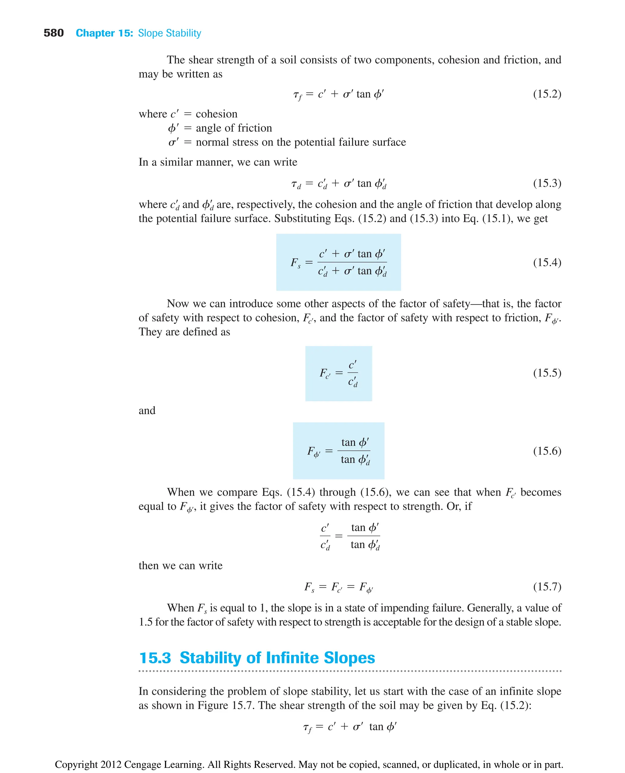
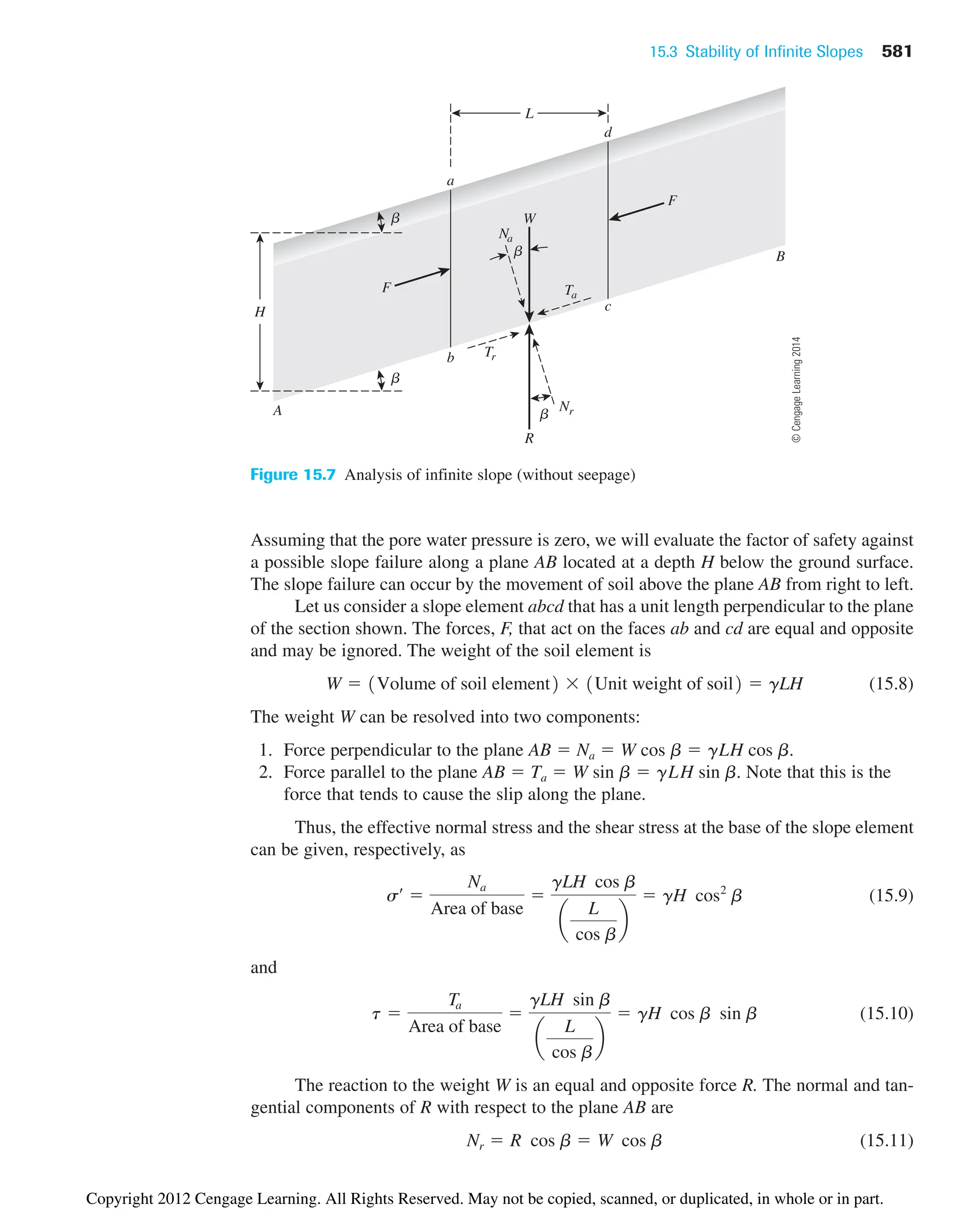
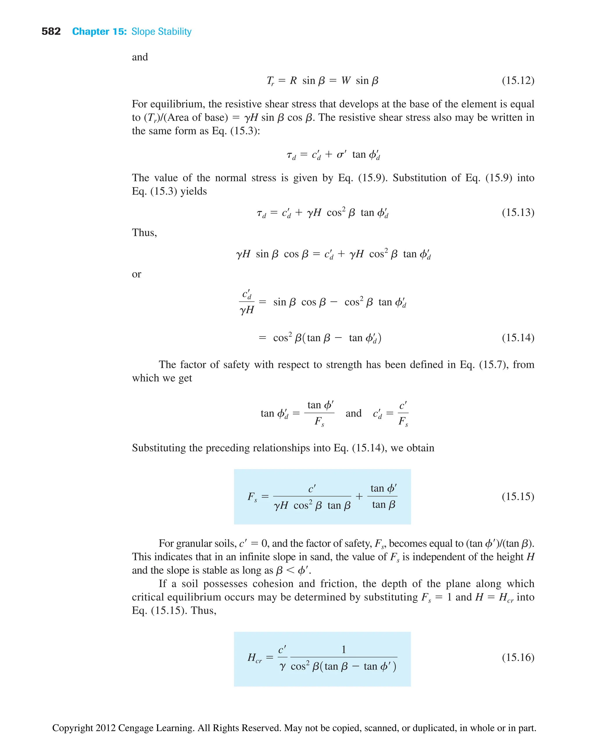
![584 Chapter 15: Slope Stability
Direction of seepage
(a)
(b)
Flow line
Equipotential line
Seepage
H cos β
H
A
H
β
β
β
h = H cos2 β
c
b
R
W
Tr
Ta
Nr
Na
a
d
c
f
b
a e
d
B
L
β
Figure 15.8 Analysis of
infinite slope (with seepage)
so
Substituting the values of s [Eq. (15.23)] and u into Eq. (15.25), we get
(15.26)
cd
œ
gœ
H cos2
b tan fd
œ
td cd
œ
1gsat H cos2
b gw H cos2
b2 tan fd
œ
u gw H cos2
b
©
Cengage
Learning
2014
Copyright 2012 Cengage Learning. All Rights Reserved. May not be copied, scanned, or duplicated, in whole or in part.](https://image.slidesharecdn.com/principlesofgeotechnicalengineering-8thedition-231222125509-7e44d9bf/75/Principles-of-Geotechnical-Engineering-8th-Edition-pdf-604-2048.jpg)
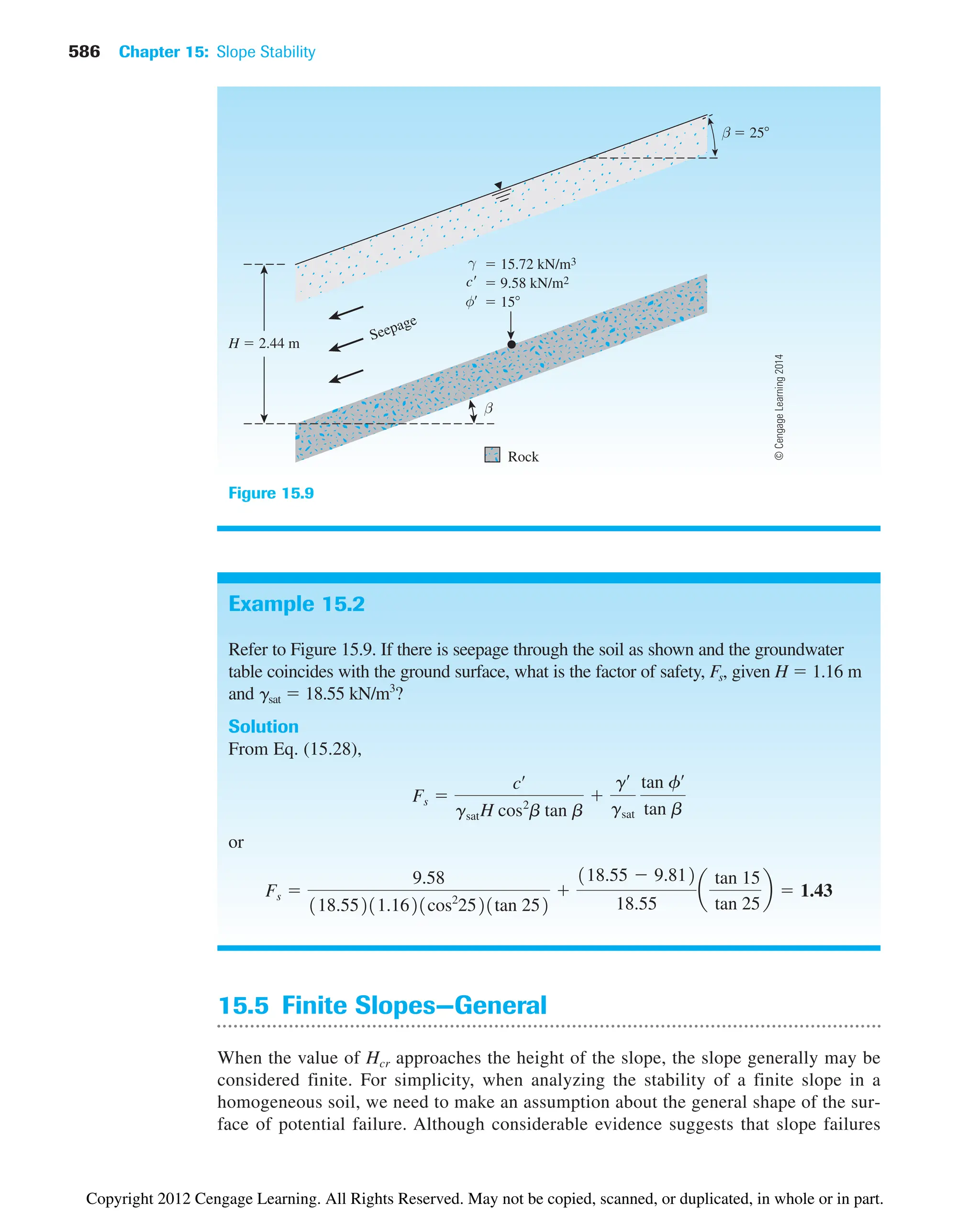
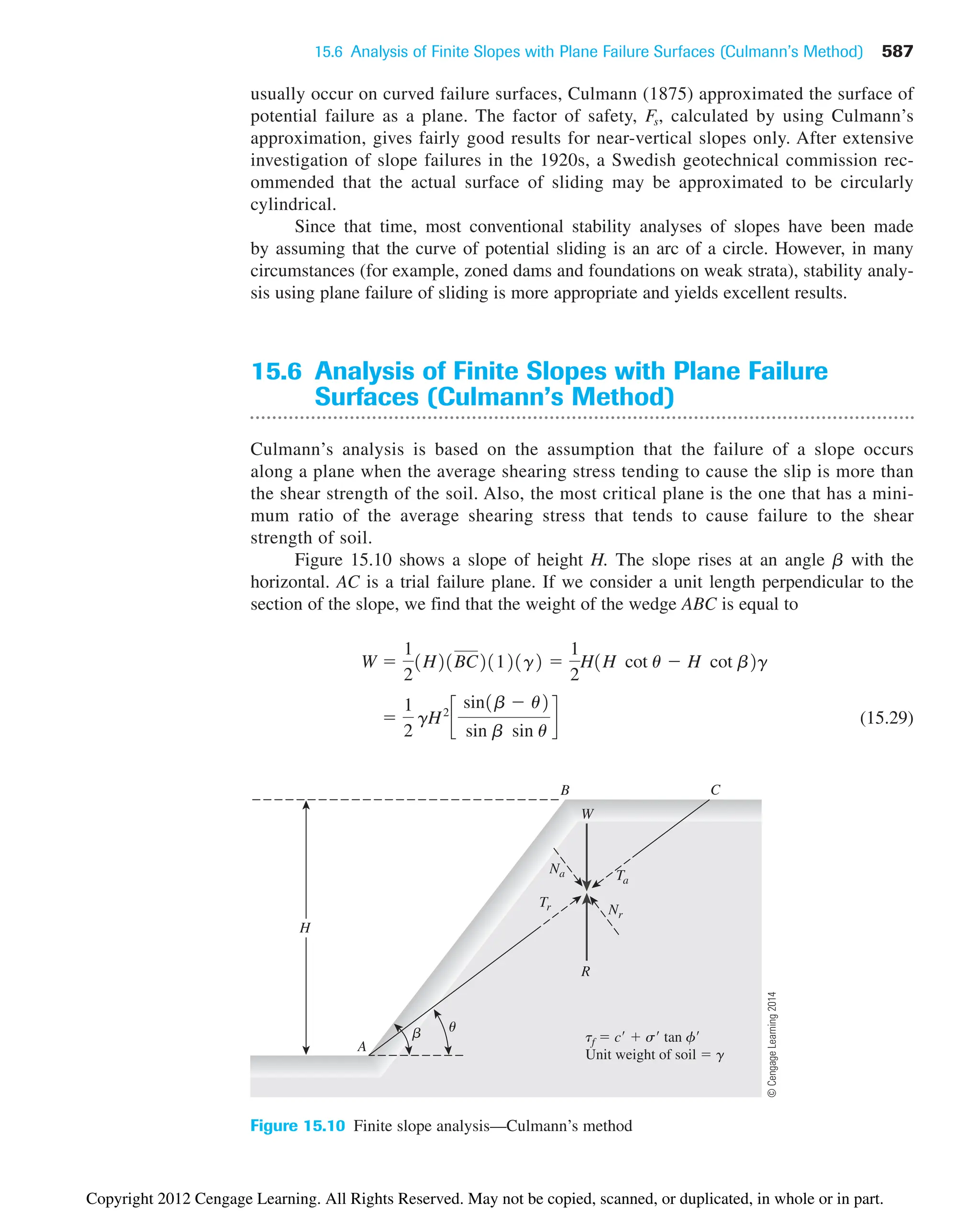
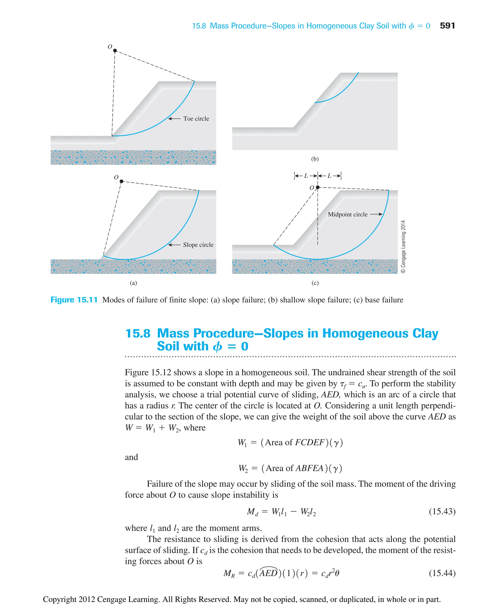
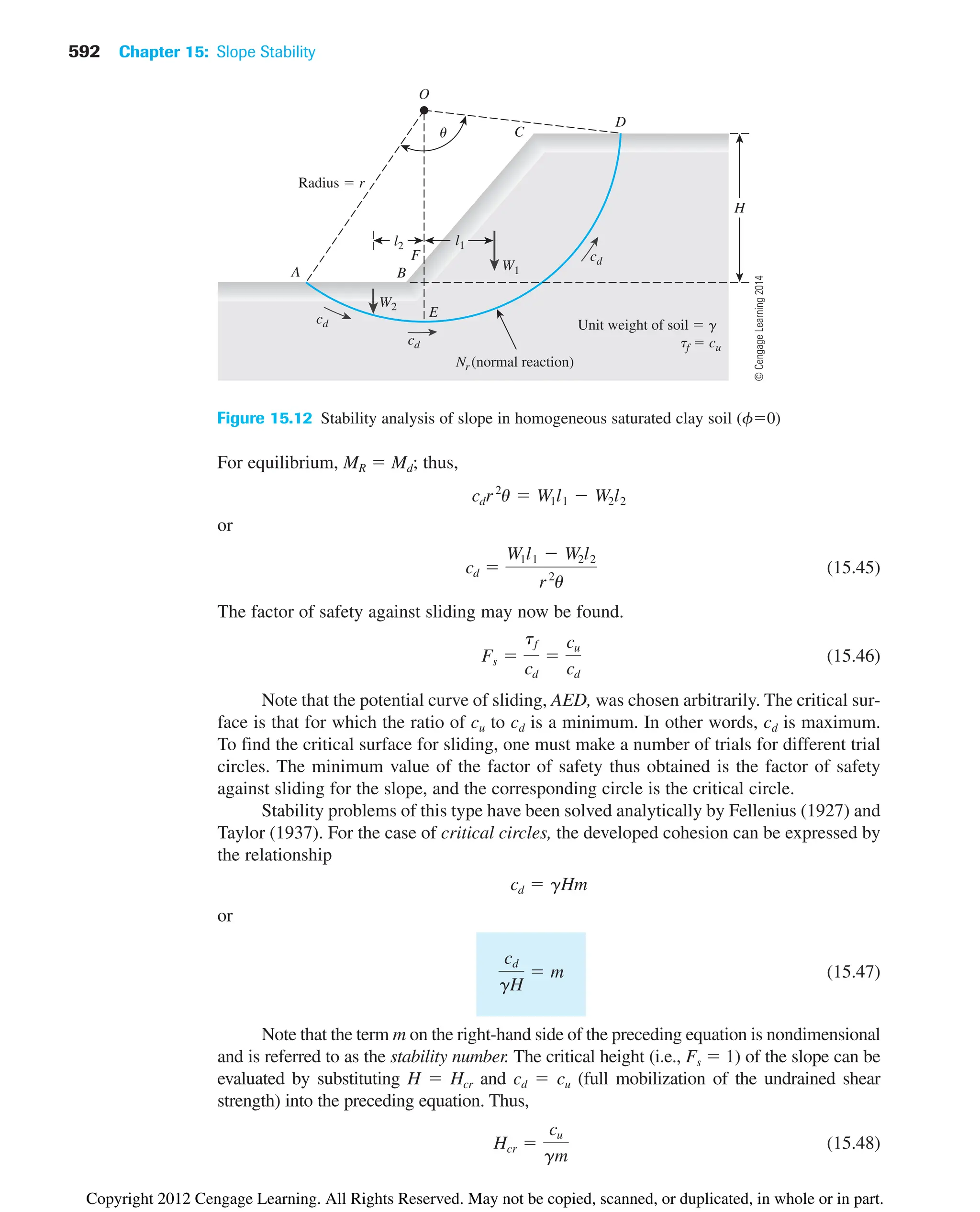
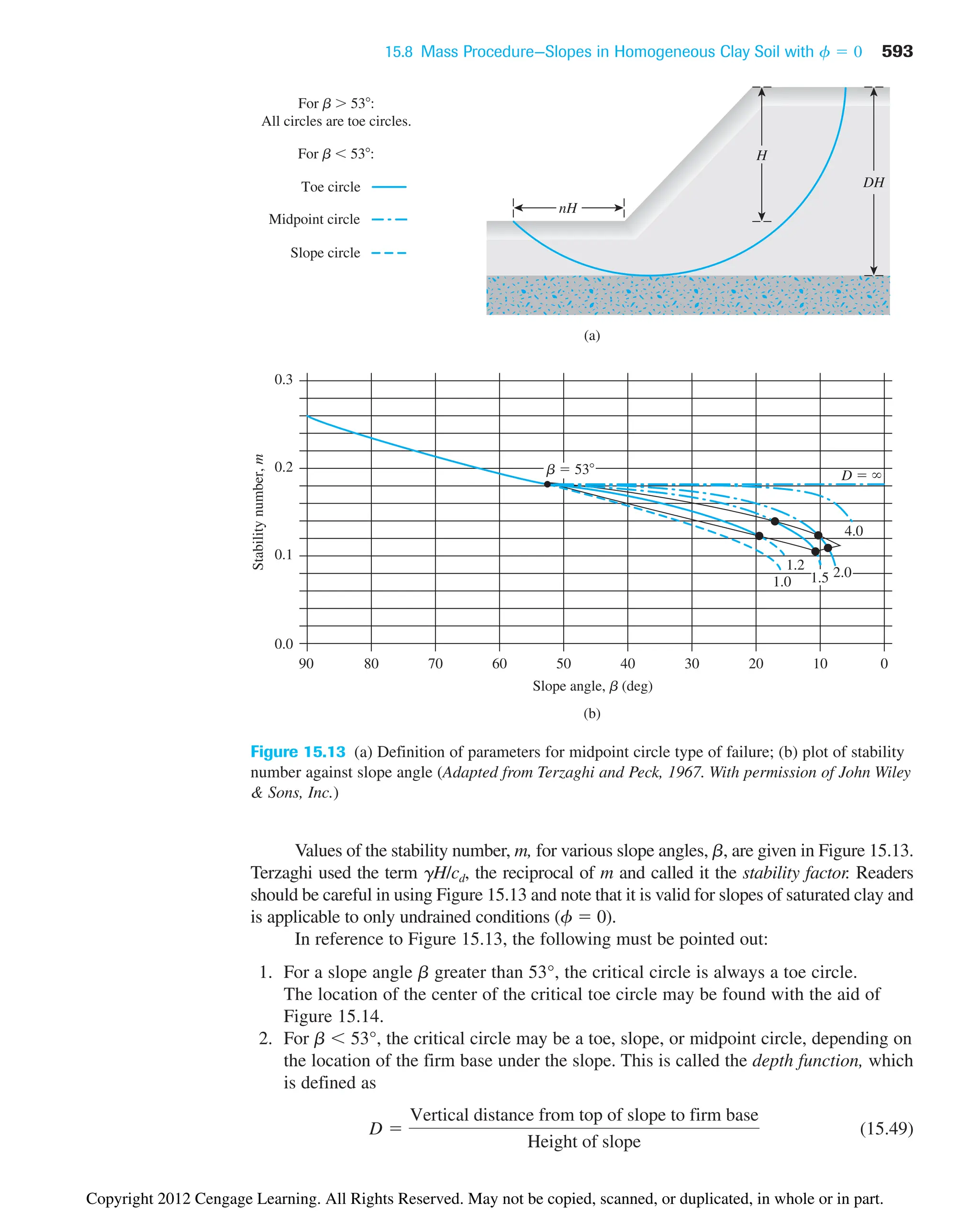
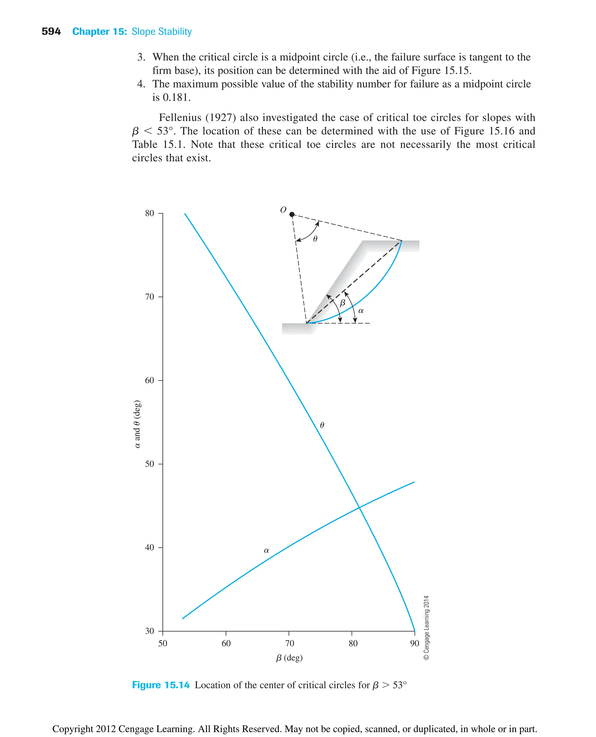
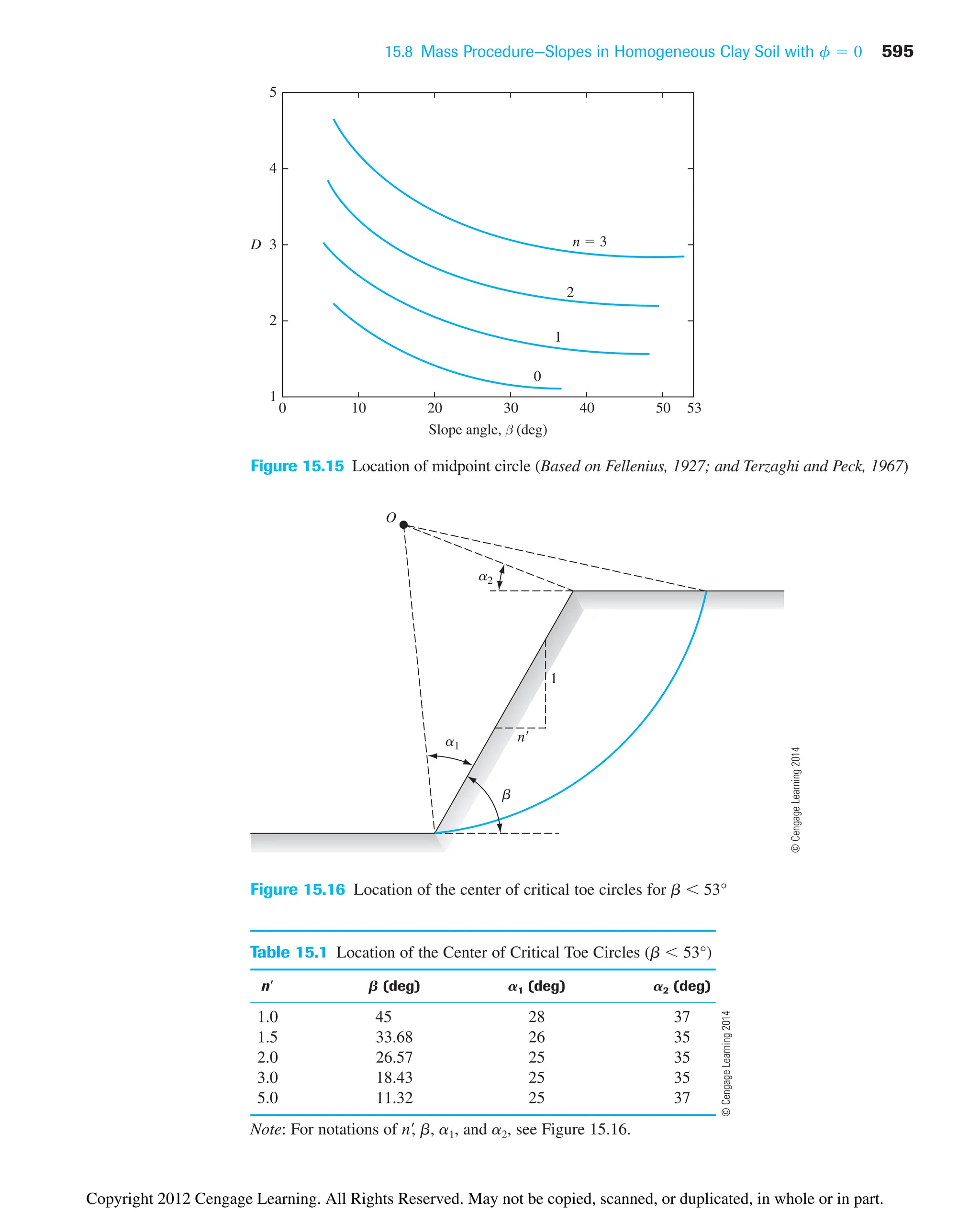
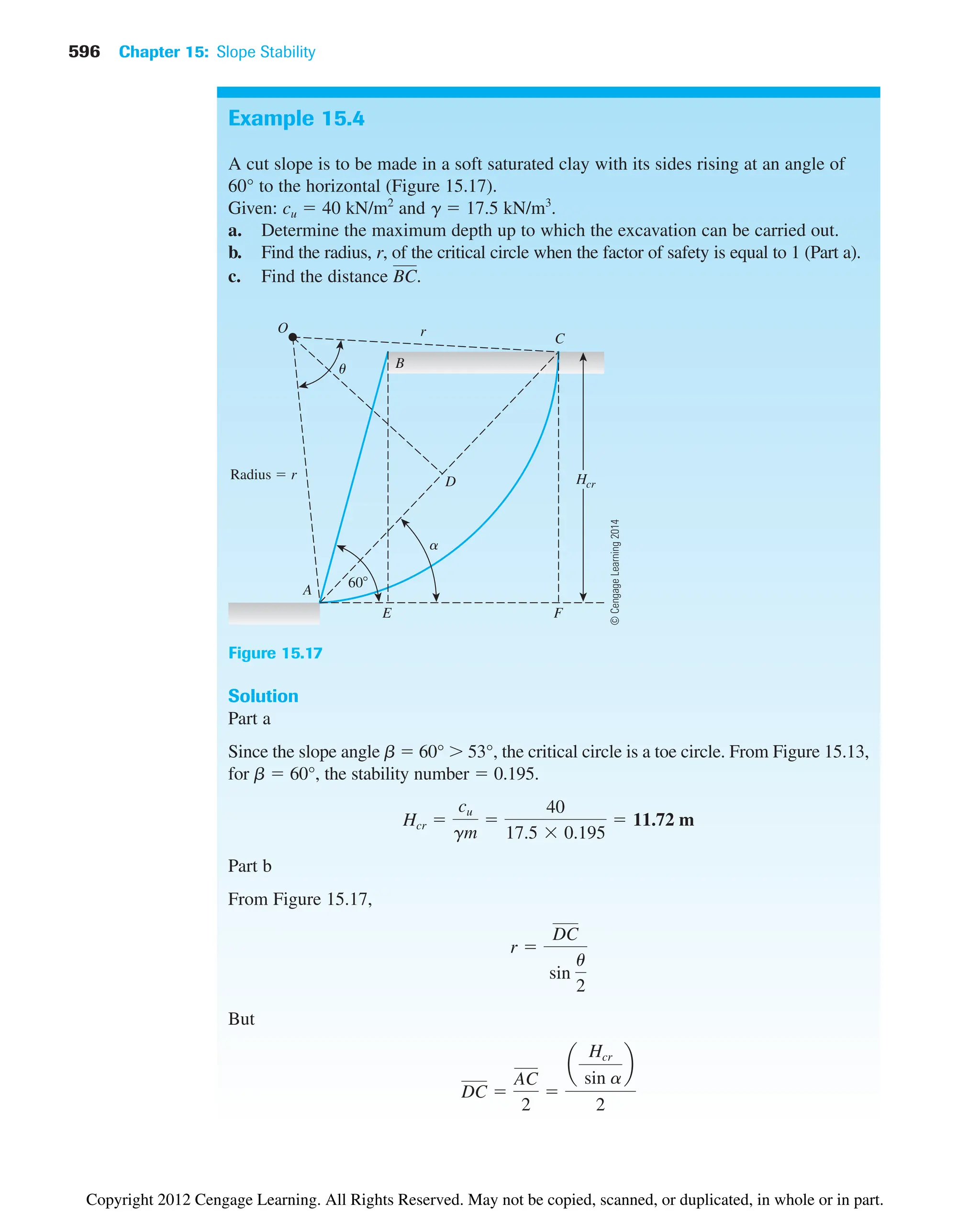
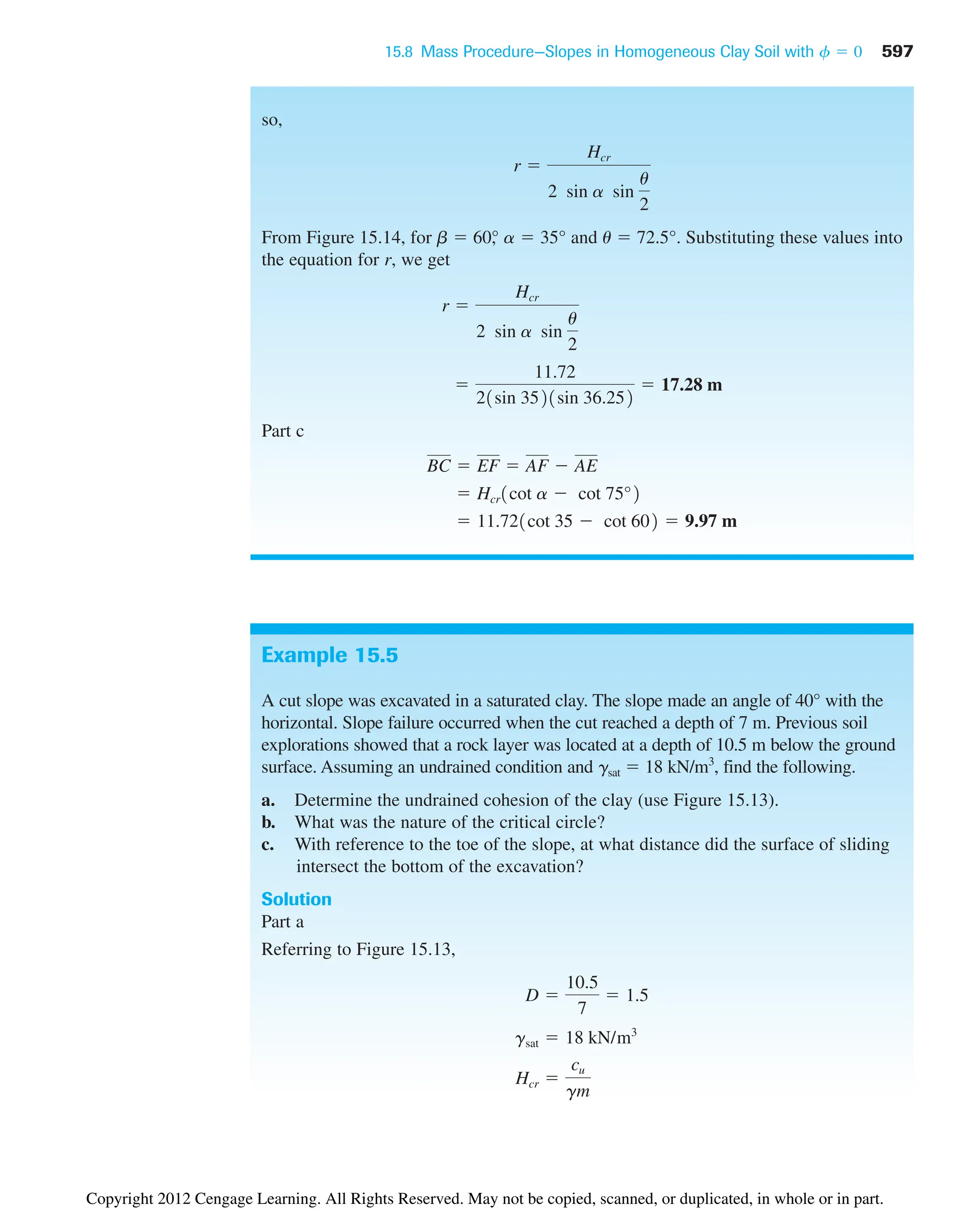
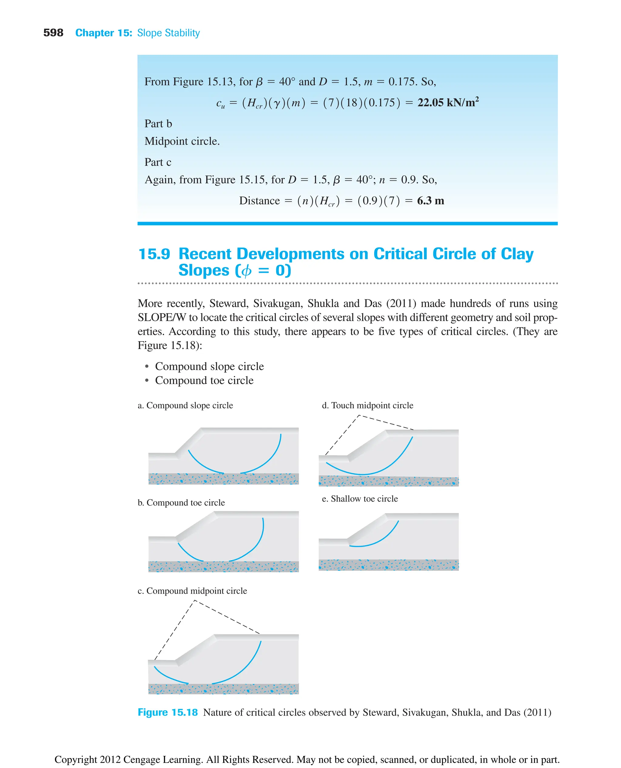
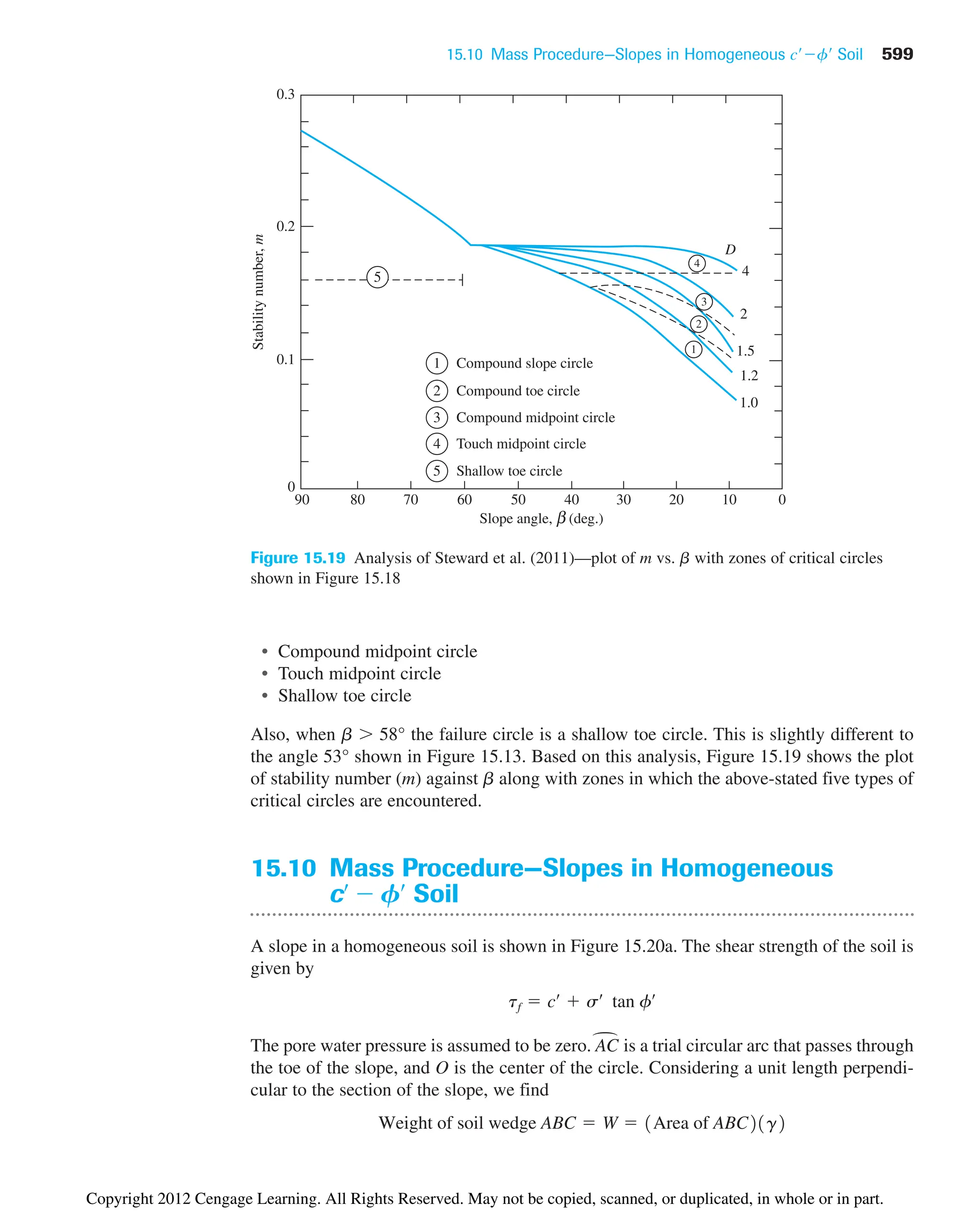
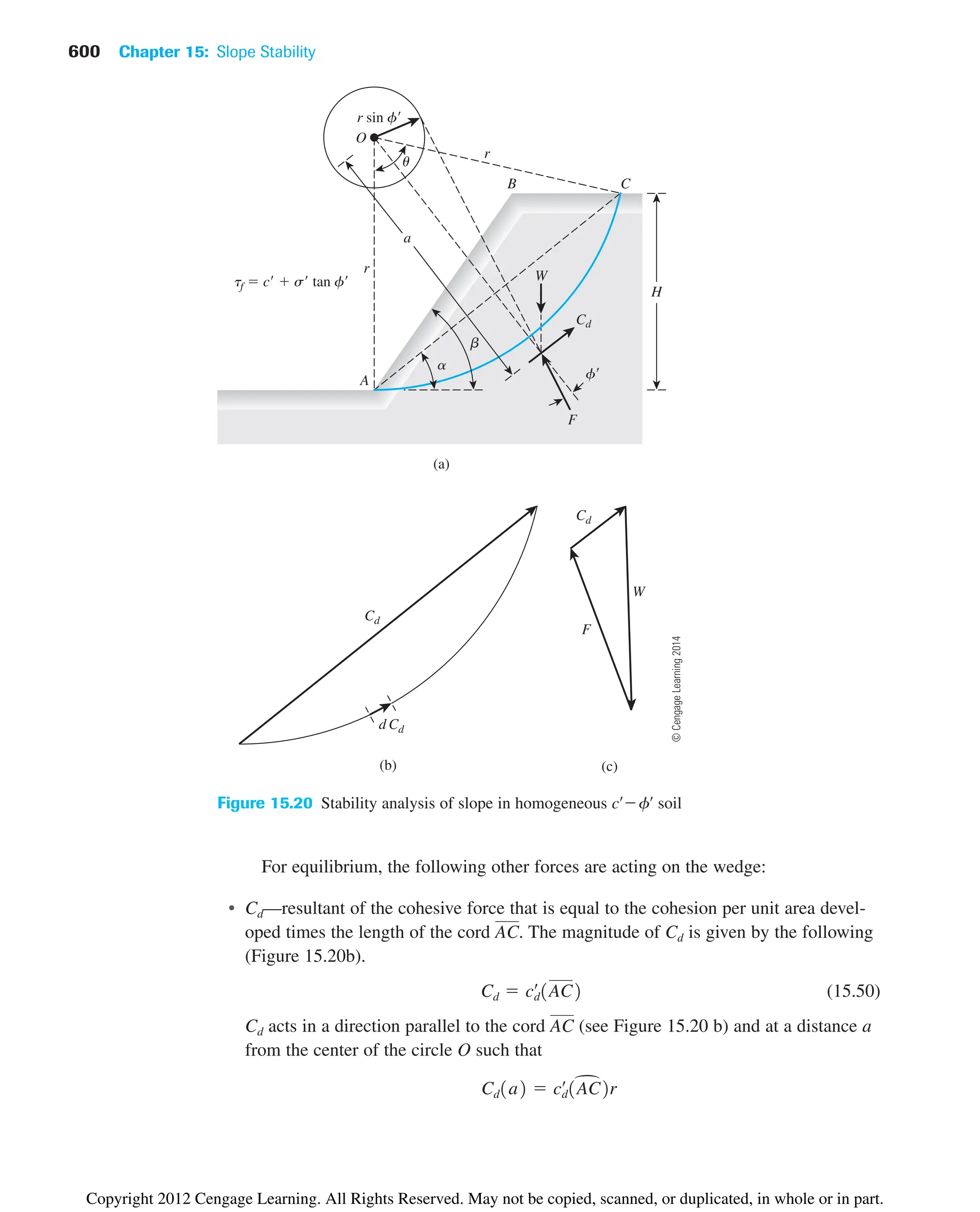
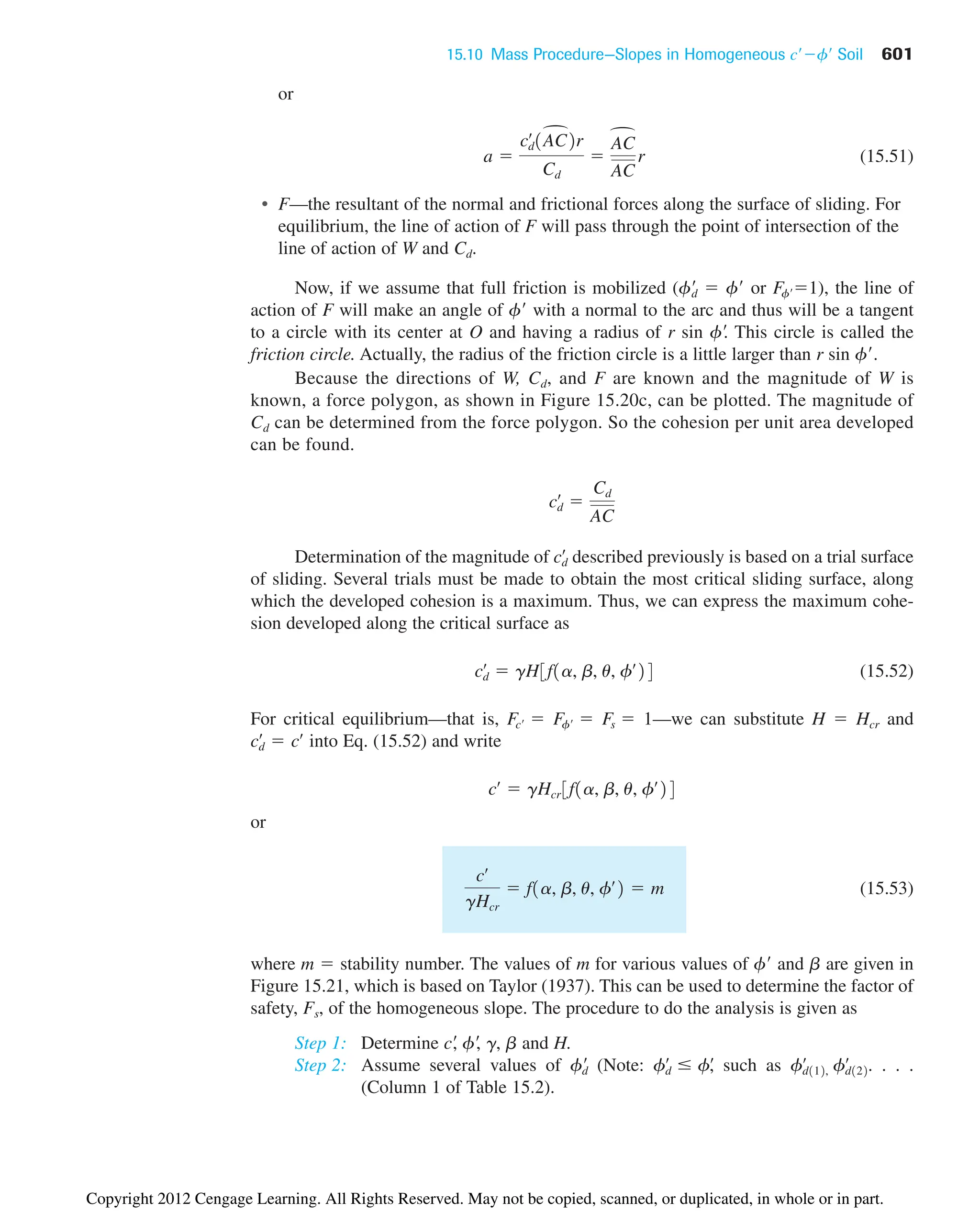
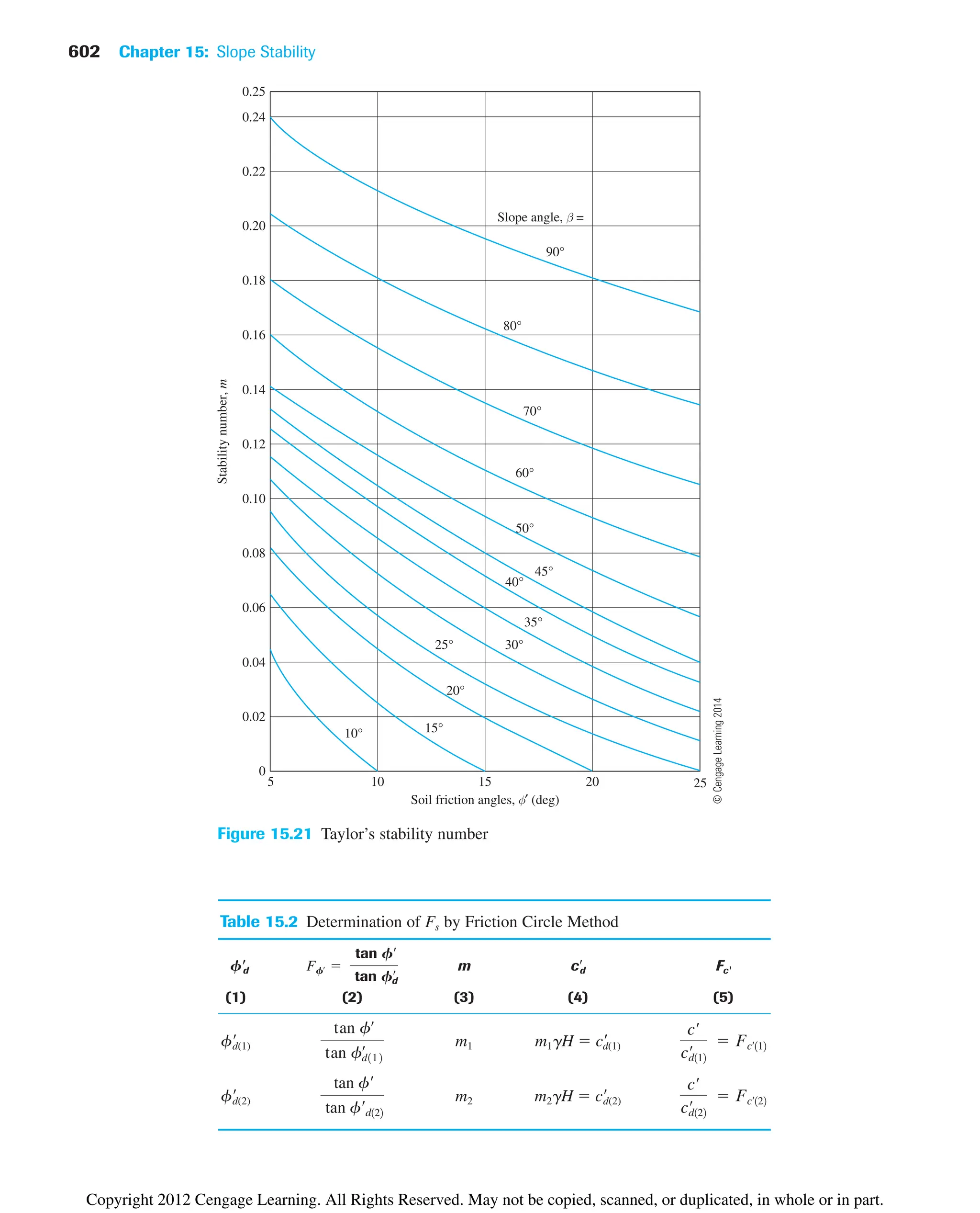
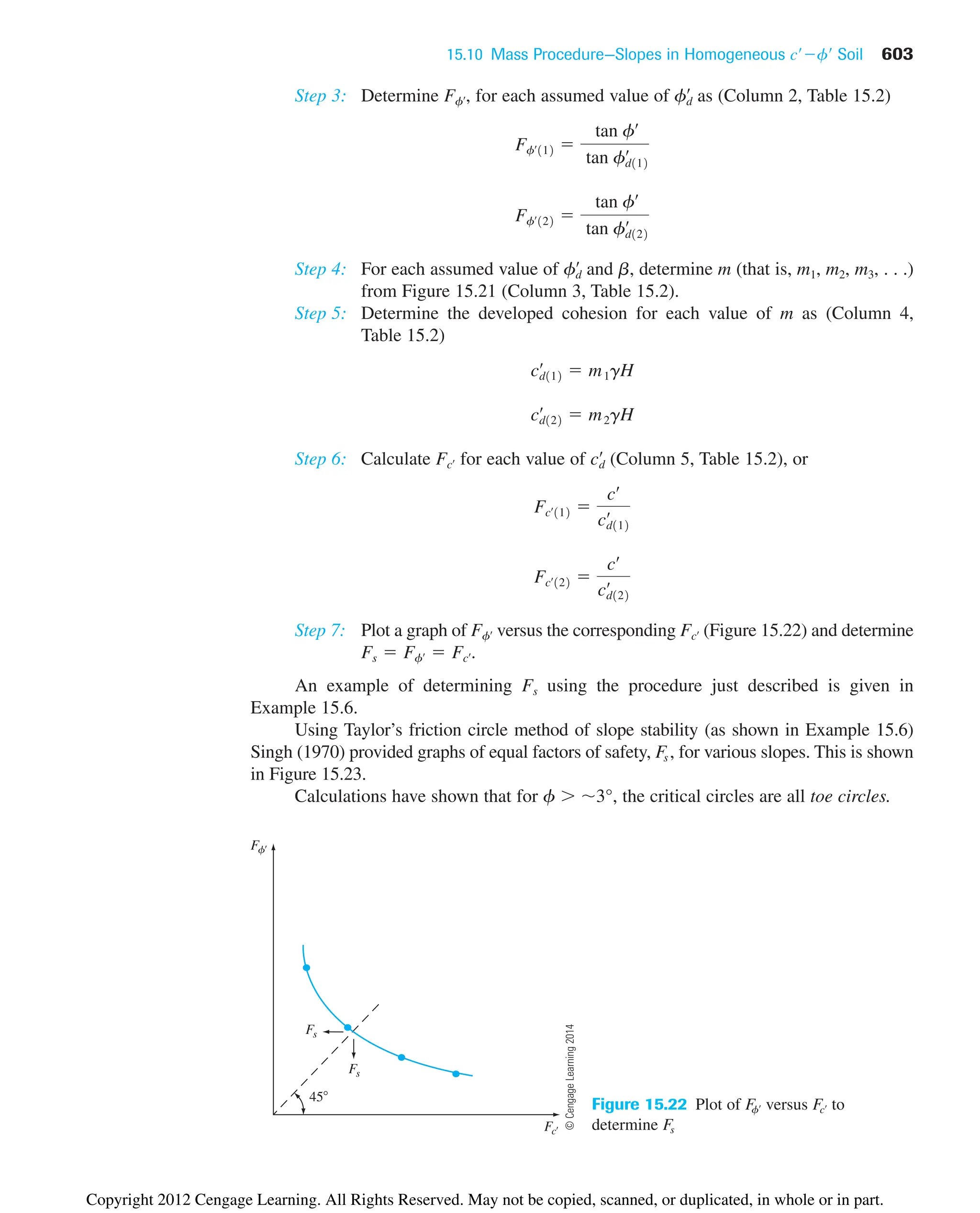
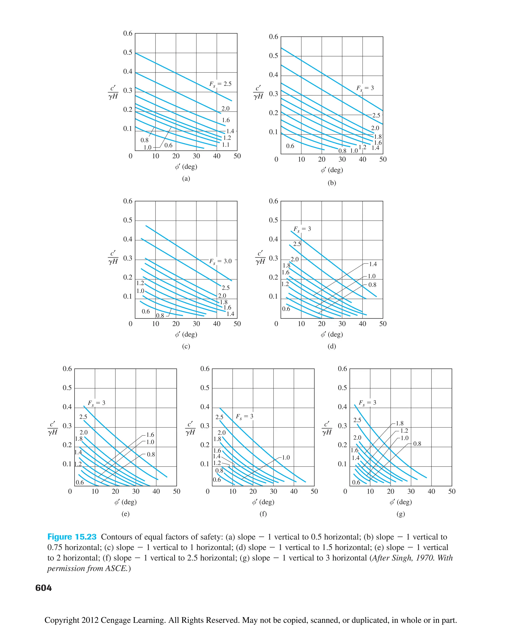
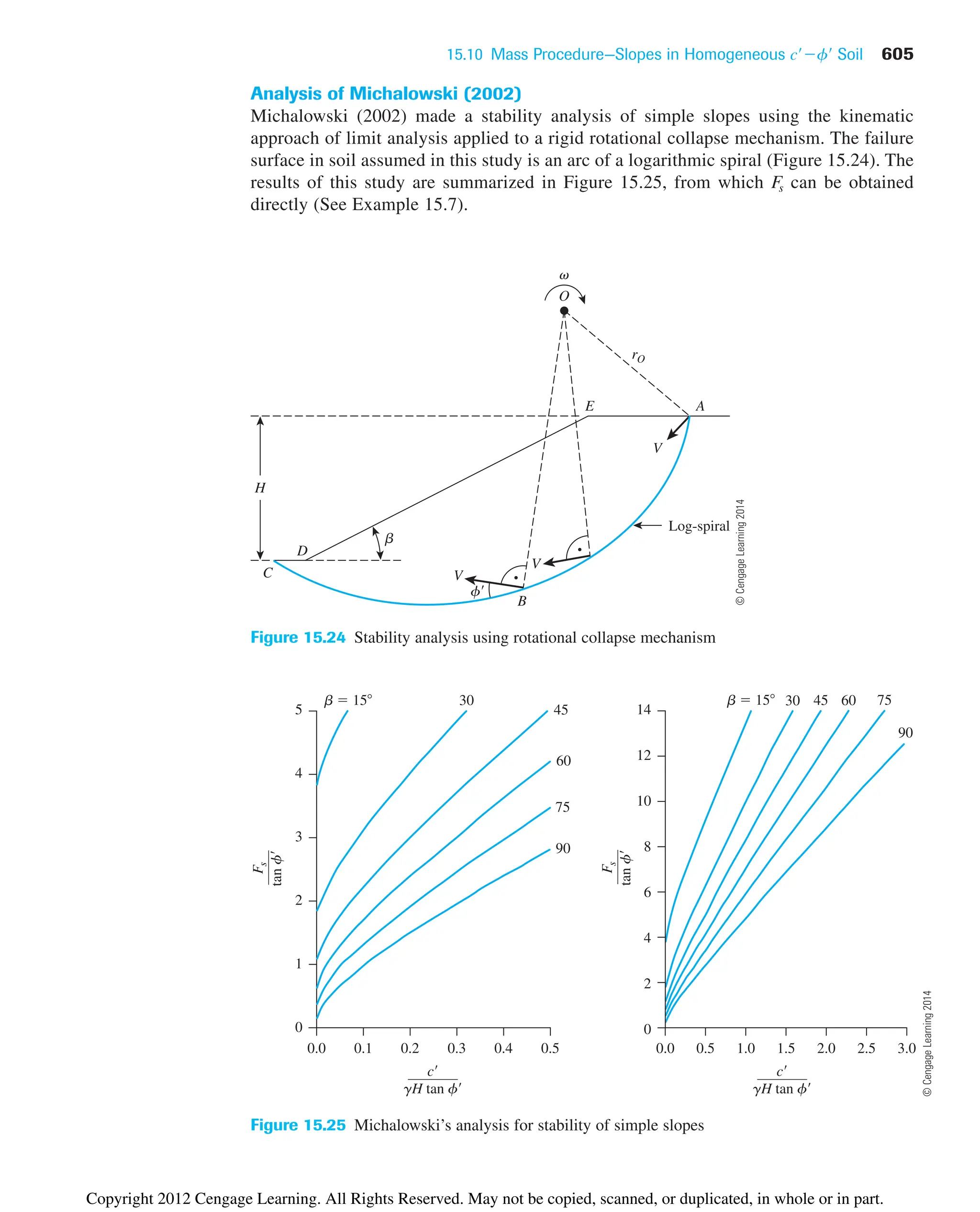
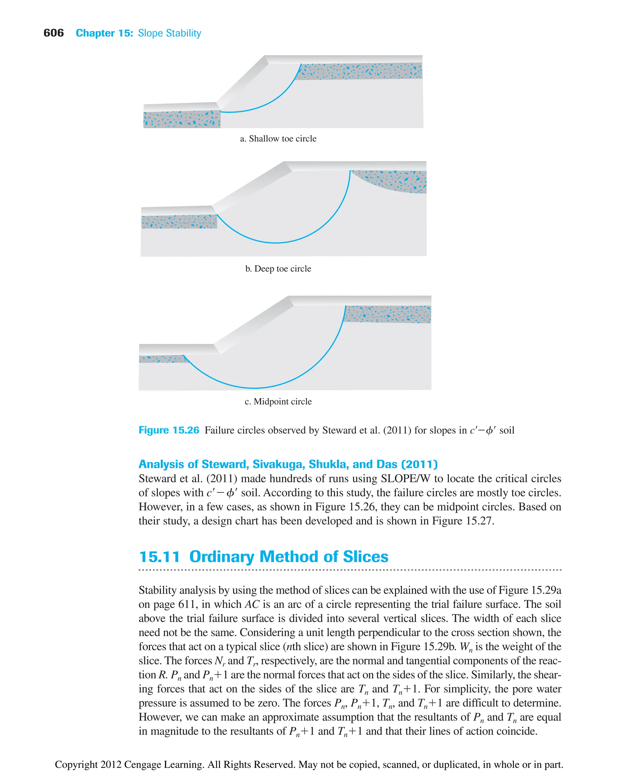
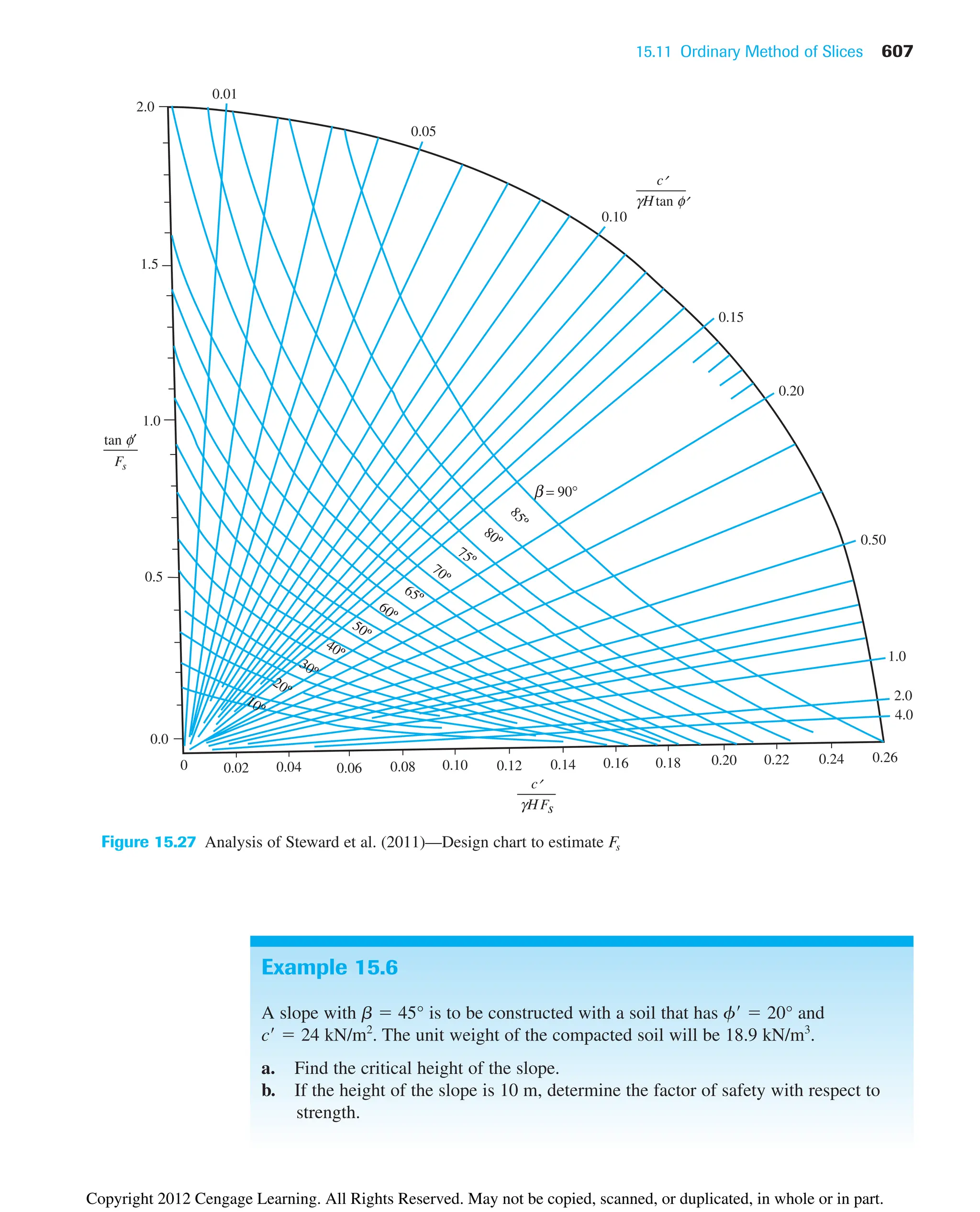
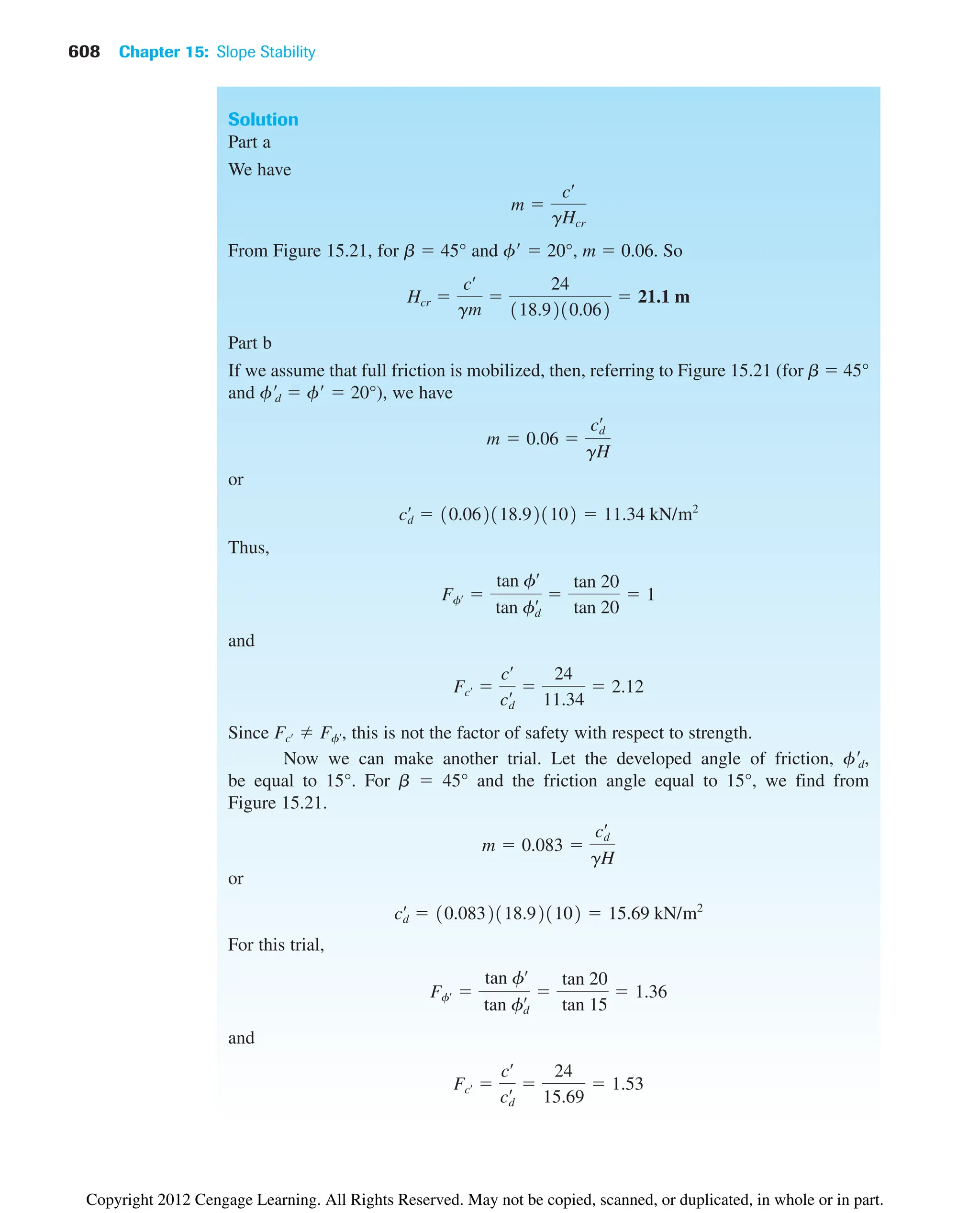
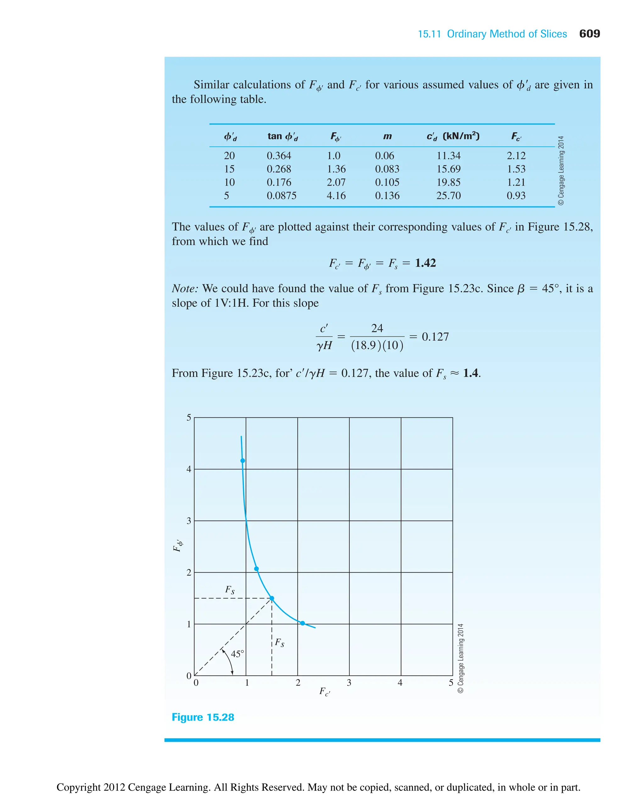
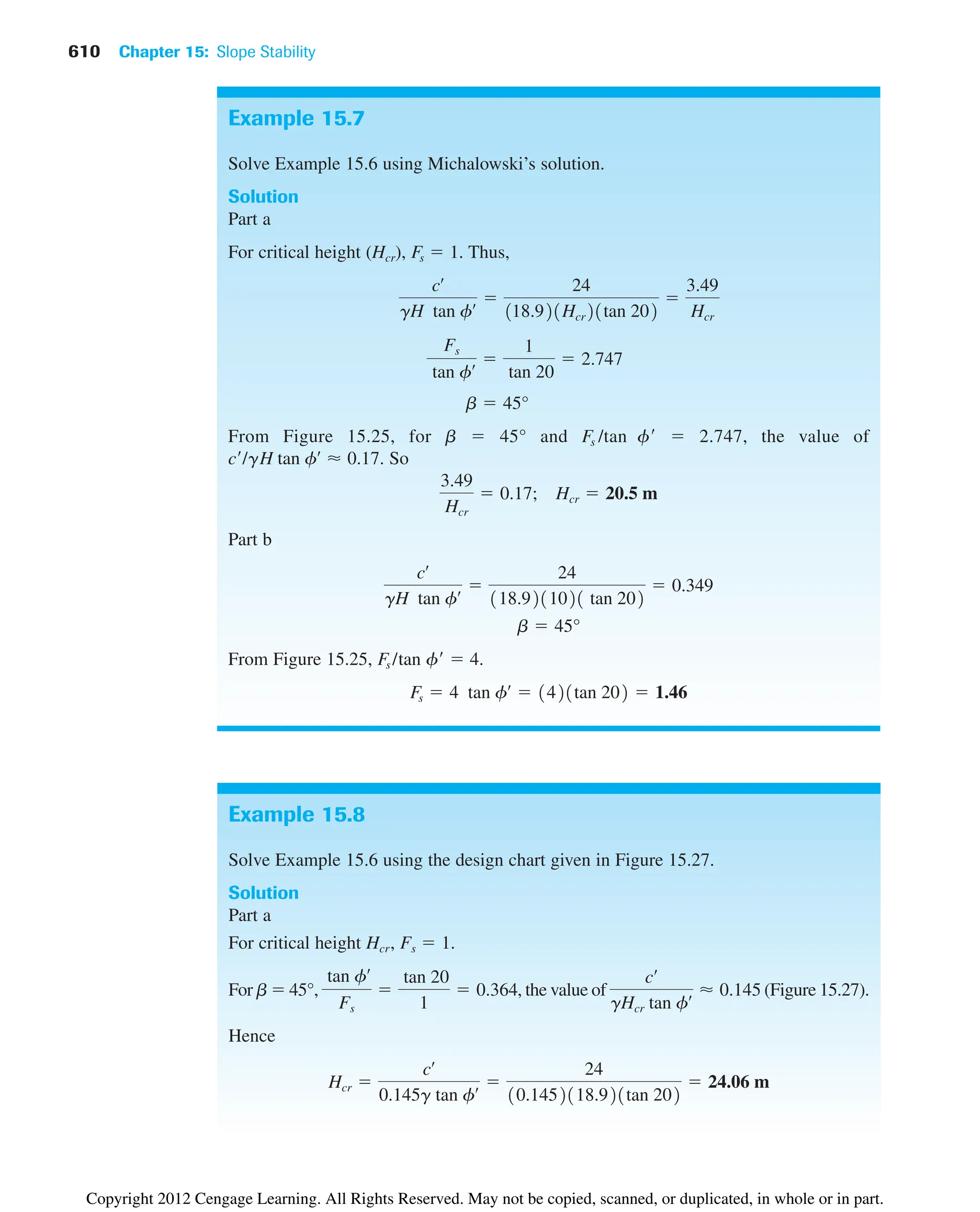
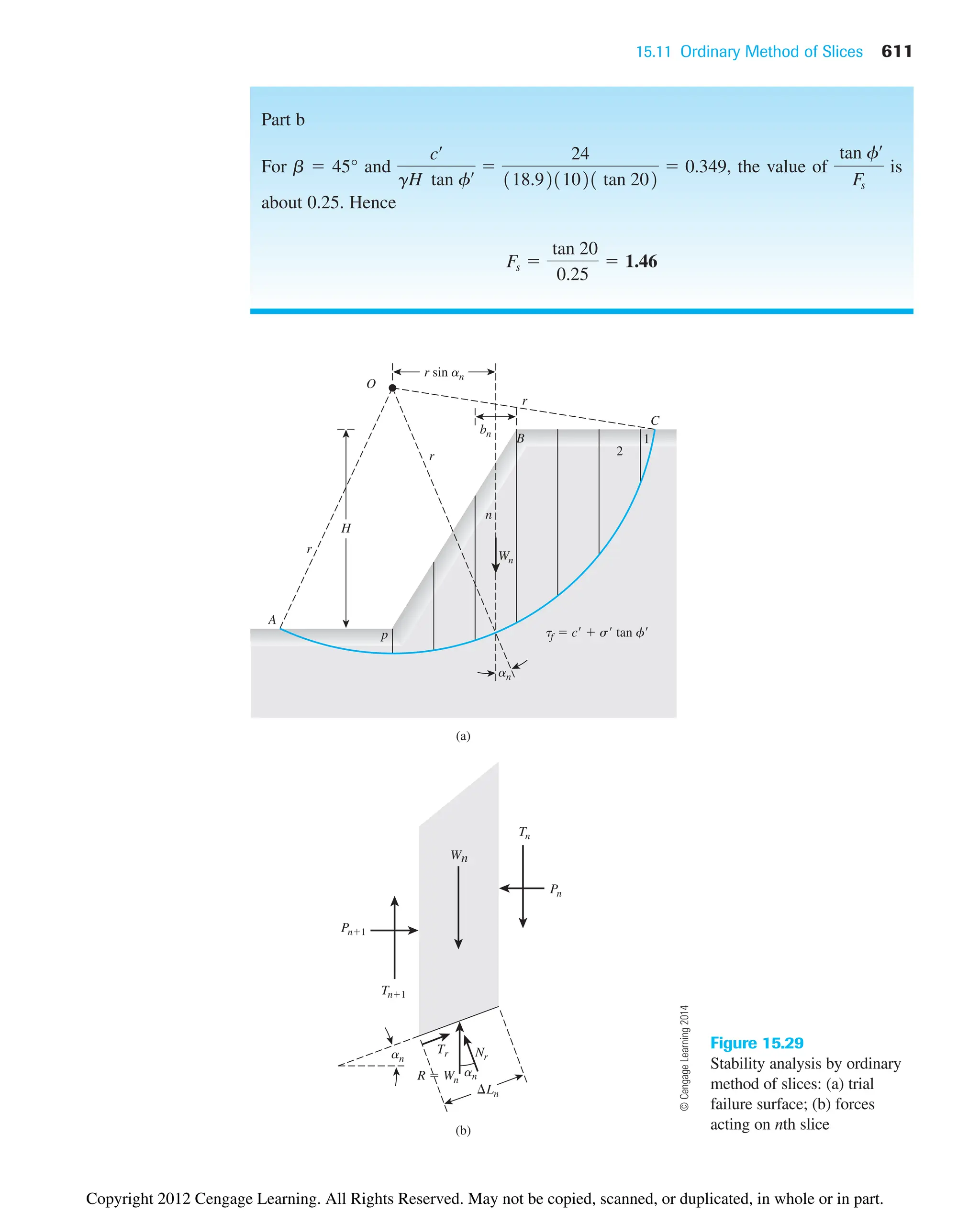
![612 Chapter 15: Slope Stability
For equilibrium consideration,
The resisting shear force can be expressed as
(15.54)
The normal stress, s, in Eq. (15.54) is equal to
For equilibrium of the trial wedge ABC, the moment of the driving force about O
equals the moment of the resisting force about O, or
or
(15.55)
[Note: Ln in Eq. (15.55) is approximately equal to (bn)/(cos an), where bn the width of
the nth slice.]
Note that the value of an may be either positive or negative. The value of an is positive
when the slope of the arc is in the same quadrant as the ground slope. To find the minimum
factor of safety—that is, the factor of safety for the critical circle—one must make several
trials by changing the center of the trial circle. This method generally is referred to as the
ordinary method of slices.
For convenience, a slope in a homogeneous soil is shown in Figure 15.29. However,
the method of slices can be extended to slopes with layered soil, as shown in Figure 15.30.
The general procedure of stability analysis is the same. However, some minor points
should be kept in mind. When Eq. (15.55) is used for the factor of safety calculation, the
values of f and c will not be the same for all slices. For example, for slice No. 3 (see
Figure 15.30), we have to use a friction angle of and cohesion ; similarly,
for slice No. 2, f f
2 and c c
2.
It is of interest to note that if total shear strength parameters (that is, tf c tan f)
were used, Eq. (15.55) would take the form
(15.56)
Fs
a
np
n1
1c¢Ln Wn cos an tan f2
a
np
n1
Wn sin an
cœ
c3
œ
fœ
f3
œ
Fs
a
np
n1
1cœ
¢Ln Wn cos an tan fœ
2
a
np
n1
Wn sin an
a
np
n1
Wnr sin an a
np
n1
1
Fs
acœ
Wn cos an
¢Ln
tan fœ
b1¢Ln21r2
Nr
¢Ln
Wn cos an
¢Ln
Tr td1¢Ln2
tf 1¢Ln2
Fs
1
Fs
3cœ
sœ
tan fœ
4¢Ln
Nr Wn cos an
Copyright 2012 Cengage Learning. All Rights Reserved. May not be copied, scanned, or duplicated, in whole or in part.](https://image.slidesharecdn.com/principlesofgeotechnicalengineering-8thedition-231222125509-7e44d9bf/75/Principles-of-Geotechnical-Engineering-8th-Edition-pdf-632-2048.jpg)
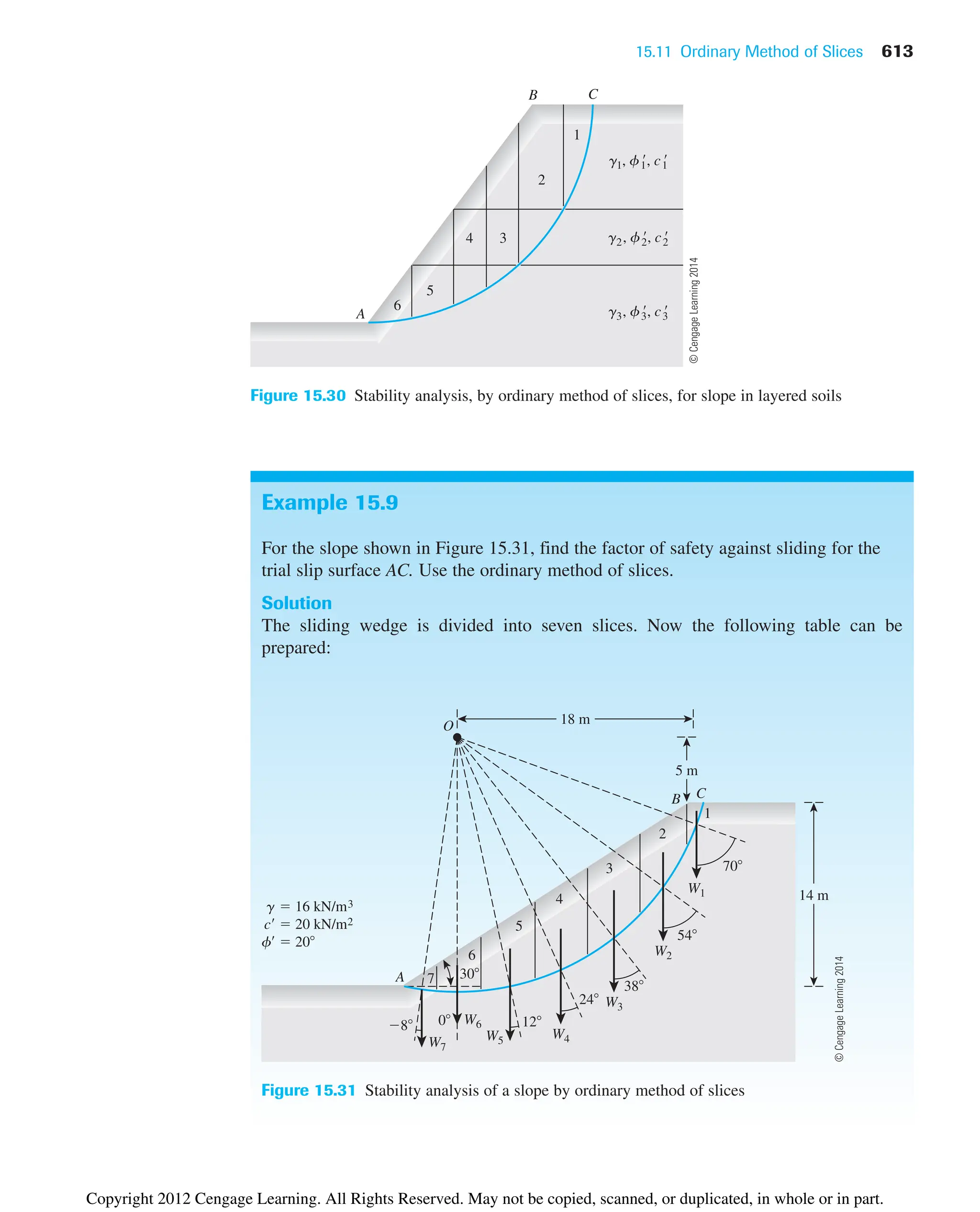
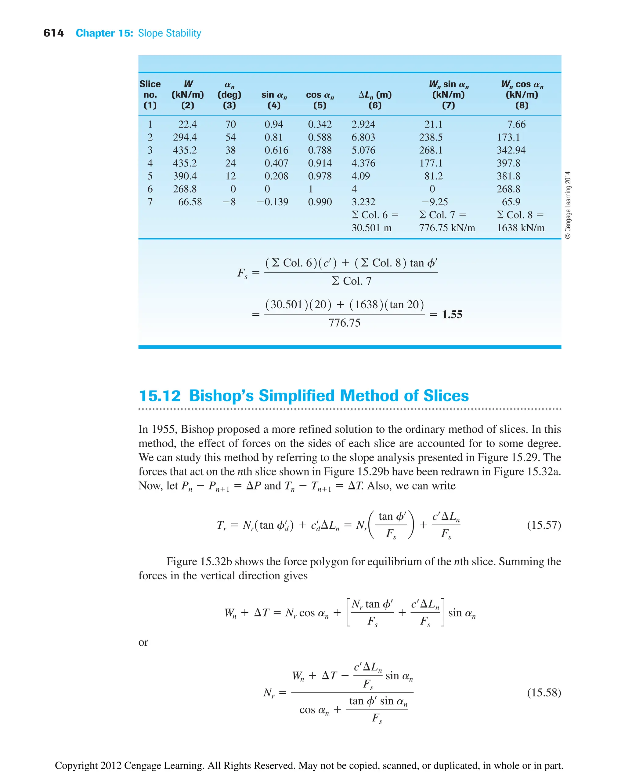
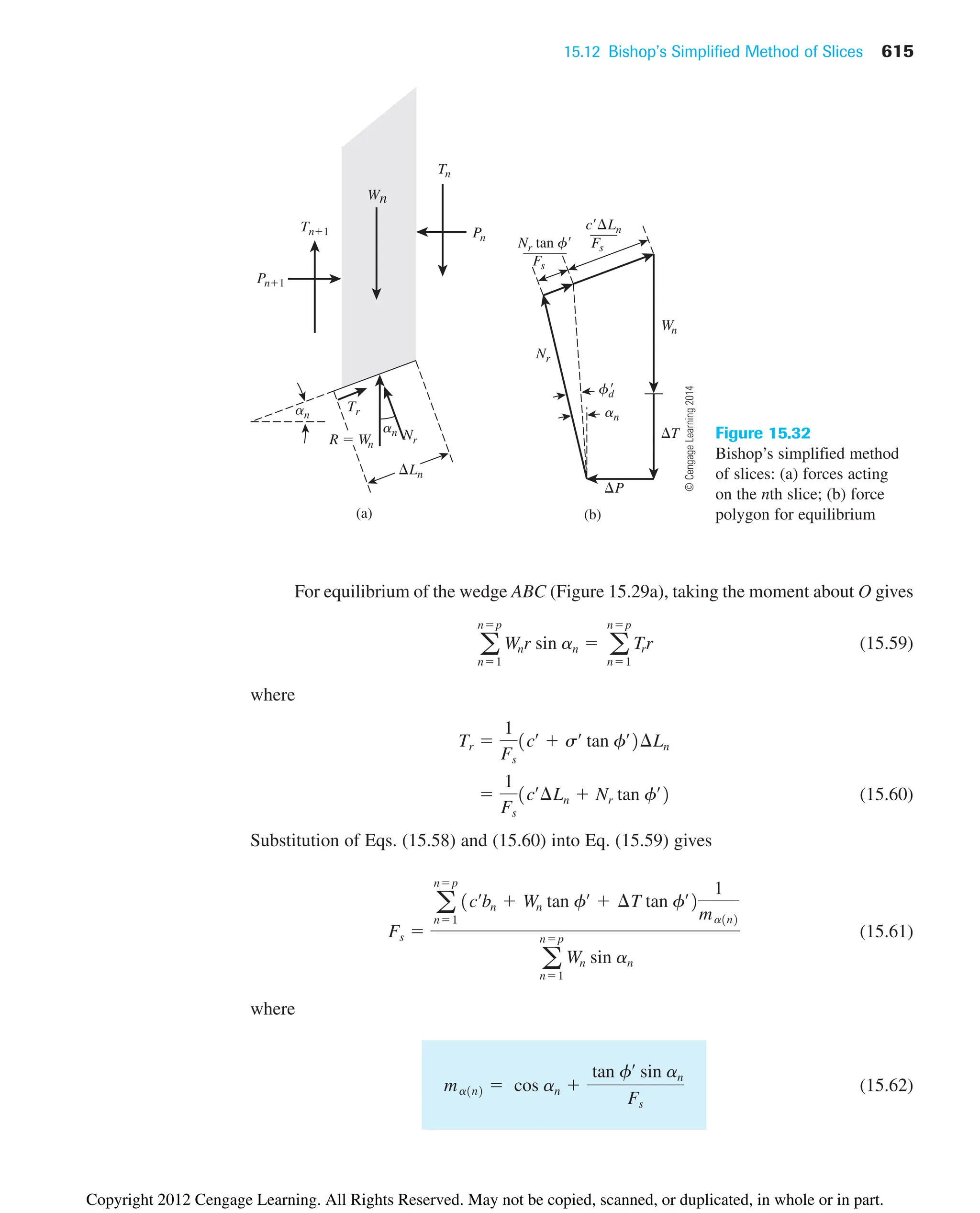
![616 Chapter 15: Slope Stability
Figure 15.33 shows the variation of ma(n) with an and tan f/Fs.
For simplicity, if we let T 0, Eq. (15.61) becomes
(15.63)
Note that the term Fs is present on both sides of Eq. (15.63). Hence, we must adopt
a trial-and-error procedure to find the value of Fs. As in the method of ordinary slices, a
number of failure surfaces must be investigated so that we can find the critical surface that
provides the minimum factor of safety.
Bishop’s simplified method is probably the most widely used. When incorporated
into computer programs, it yields satisfactory results in most cases. The ordinary method
of slices is presented in this chapter as a learning tool only. It is used rarely now because
it is too conservative.
15.13 Stability Analysis by Method of Slices for
Steady-state Seepage
The fundamentals of the ordinary method of slices and Bishop’s simplified method of slices
were presented in Sections 15.11 and 15.12, respectively, and we assumed the pore water
pressure to be zero. However, for steady-state seepage through slopes, as is the situation in
many practical cases, the pore water pressure must be considered when effective shear
strength parameters are used. So we need to modify Eqs. (15.55) and (15.63) slightly.
Figure 15.34 shows a slope through which there is steady-state seepage. For the nth
slice, the average pore water pressure at the bottom of the slice is equal to un hngw. The
total force caused by the pore water pressure at the bottom of the nth slice is equal to un Ln.
Fs
a
np
n1
1cœ
bn Wn tan fœ
2
1
ma1n2
a
np
n1
Wn sin an
Figure 15.33 Variation of ma(n)
with an and tan f/Fs [Eq. (15.62)]
©
Cengage
Learning
2014
Copyright 2012 Cengage Learning. All Rights Reserved. May not be copied, scanned, or duplicated, in whole or in part.](https://image.slidesharecdn.com/principlesofgeotechnicalengineering-8thedition-231222125509-7e44d9bf/75/Principles-of-Geotechnical-Engineering-8th-Edition-pdf-636-2048.jpg)
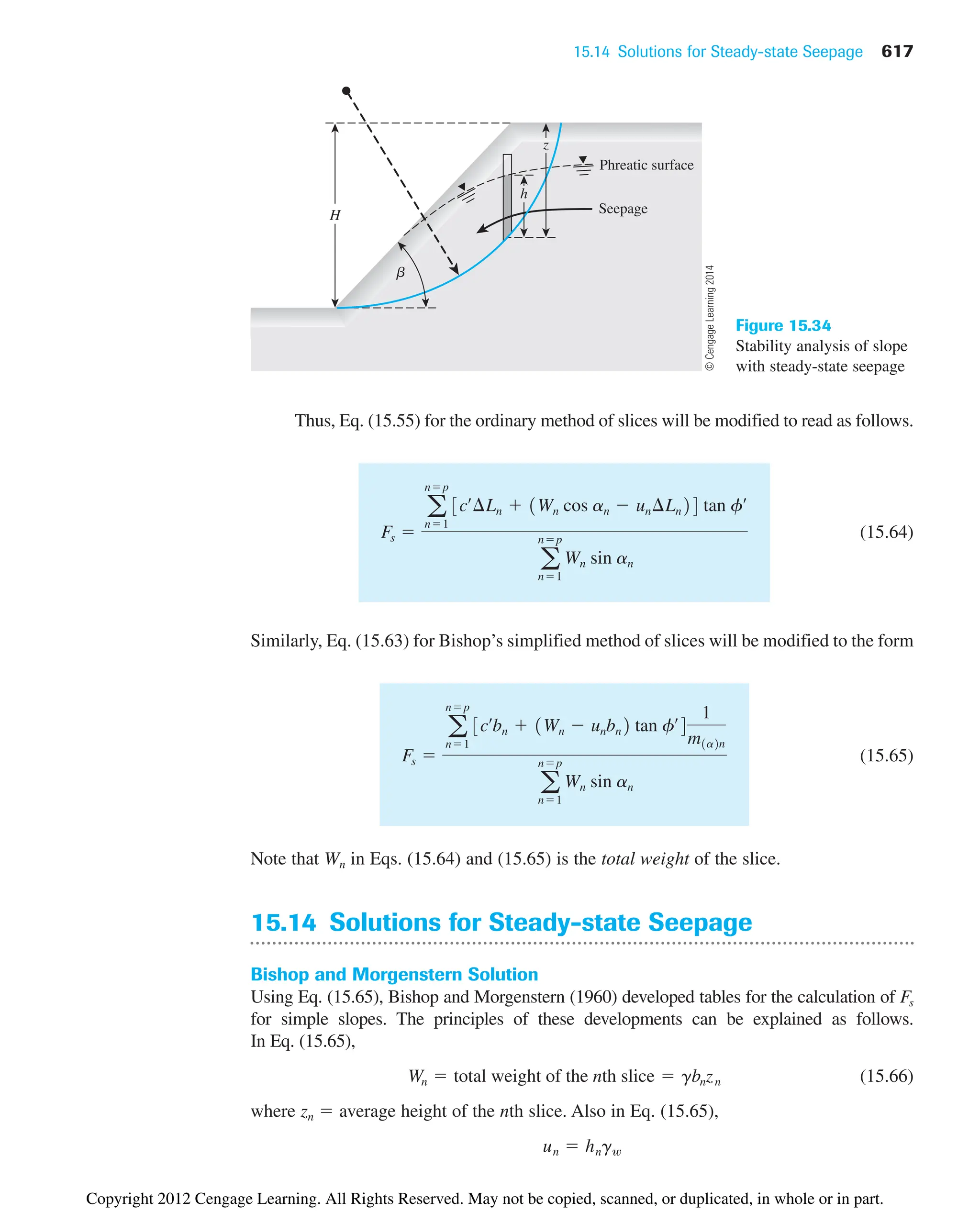
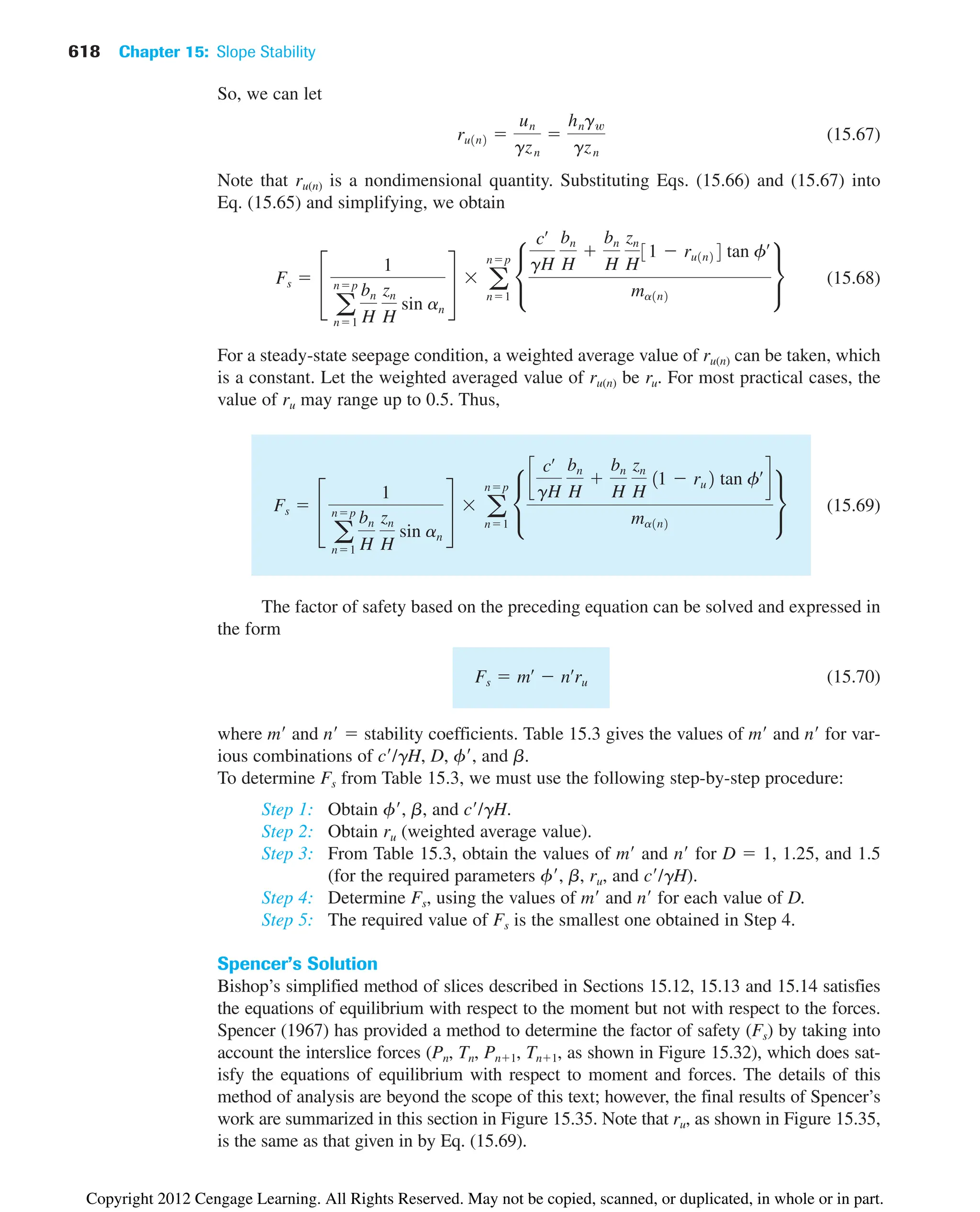
![15.14 Solutions for Steady-state Seepage 619
Table 15.3 Values of m and n [Eq. (15.70)]
a. Stability coefficients m and n for c/g H ⴝ 0
Stability coefficients for earth slopes
Slope 2:1 Slope 3:1 Slope 4:1 Slope 5:1
f m n m n m n m n
10.0 0.353 0.441 0.529 0.588 0.705 0.749 0.882 0.917
12.5 0.443 0.554 0.665 0.739 0.887 0.943 1.109 1.153
15.0 0.536 0.670 0.804 0.893 1.072 1.139 1.340 1.393
17.5 0.631 0.789 0.946 1.051 1.261 1.340 1.577 1.639
20.0 0.728 0.910 1.092 1.213 1.456 1.547 1.820 1.892
22.5 0.828 1.035 1.243 1.381 1.657 1.761 2.071 2.153
25.0 0.933 1.166 1.399 1.554 1.865 1.982 2.332 2.424
27.5 1.041 1.301 1.562 1.736 2.082 2.213 2.603 2.706
30.0 1.155 1.444 1.732 1.924 2.309 2.454 2.887 3.001
32.5 1.274 1.593 1.911 2.123 2.548 2.708 3.185 3.311
35.0 1.400 1.750 2.101 2.334 2.801 2.977 3.501 3.639
37.5 1.535 1.919 2.302 2.558 3.069 3.261 3.837 3.989
40.0 1.678 2.098 2.517 2.797 3.356 3.566 4.196 4.362
b. Stability coefficients m and n for c/g H ⴝ 0.025 and D ⴝ 1.00
Stability coefficients for earth slopes
Slope 2:1 Slope 3:1 Slope 4:1 Slope 5:1
f m n m n m n m n
10.0 0.678 0.534 0.906 0.683 1.130 0.846 1.367 1.031
12.5 0.790 0.655 1.066 0.849 1.337 1.061 1.620 1.282
15.0 0.901 0.776 1.224 1.014 1.544 1.273 1.868 1.534
17.5 1.012 0.898 1.380 1.179 1.751 1.485 2.121 1.789
20.0 1.124 1.022 1.542 1.347 1.962 1.698 2.380 2.050
22.5 1.239 1.150 1.705 1.518 2.177 1.916 2.646 2.317
25.0 1.356 1.282 1.875 1.696 2.400 2.141 2.921 2.596
27.5 1.478 1.421 2.050 1.882 2.631 2.375 3.207 2.886
30.0 1.606 1.567 2.235 2.078 2.873 2.622 3.508 3.191
32.5 1.739 1.721 2.431 2.285 3.127 2.883 3.823 3.511
35.0 1.880 1.885 2.635 2.505 3.396 3.160 4.156 3.849
37.5 2.030 2.060 2.855 2.741 3.681 3.458 4.510 4.209
40.0 2.190 2.247 3.090 2.993 3.984 3.778 4.885 4.592
(continued)
©
Cengage
Learning
2014
Copyright 2012 Cengage Learning. All Rights Reserved. May not be copied, scanned, or duplicated, in whole or in part.](https://image.slidesharecdn.com/principlesofgeotechnicalengineering-8thedition-231222125509-7e44d9bf/75/Principles-of-Geotechnical-Engineering-8th-Edition-pdf-639-2048.jpg)
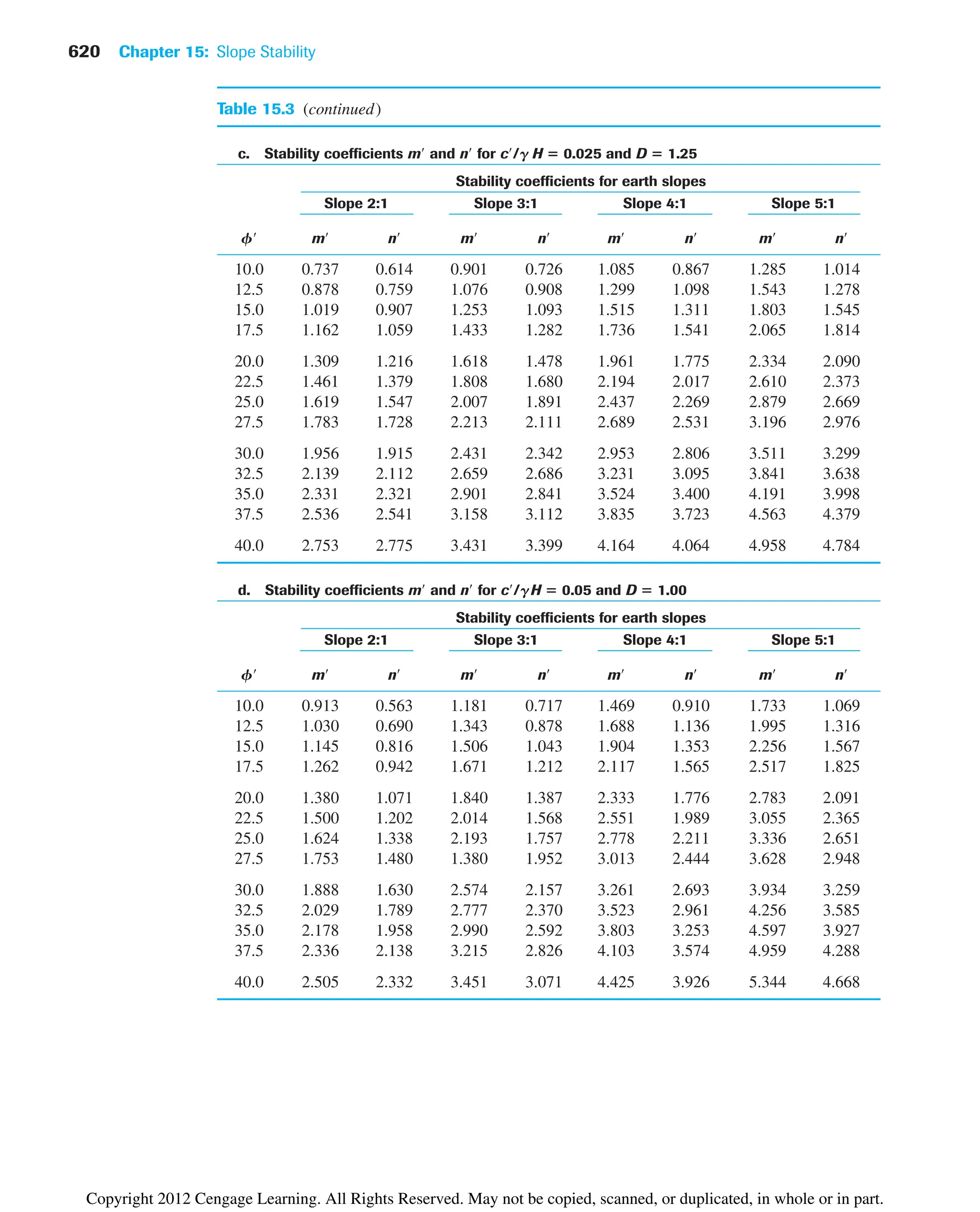
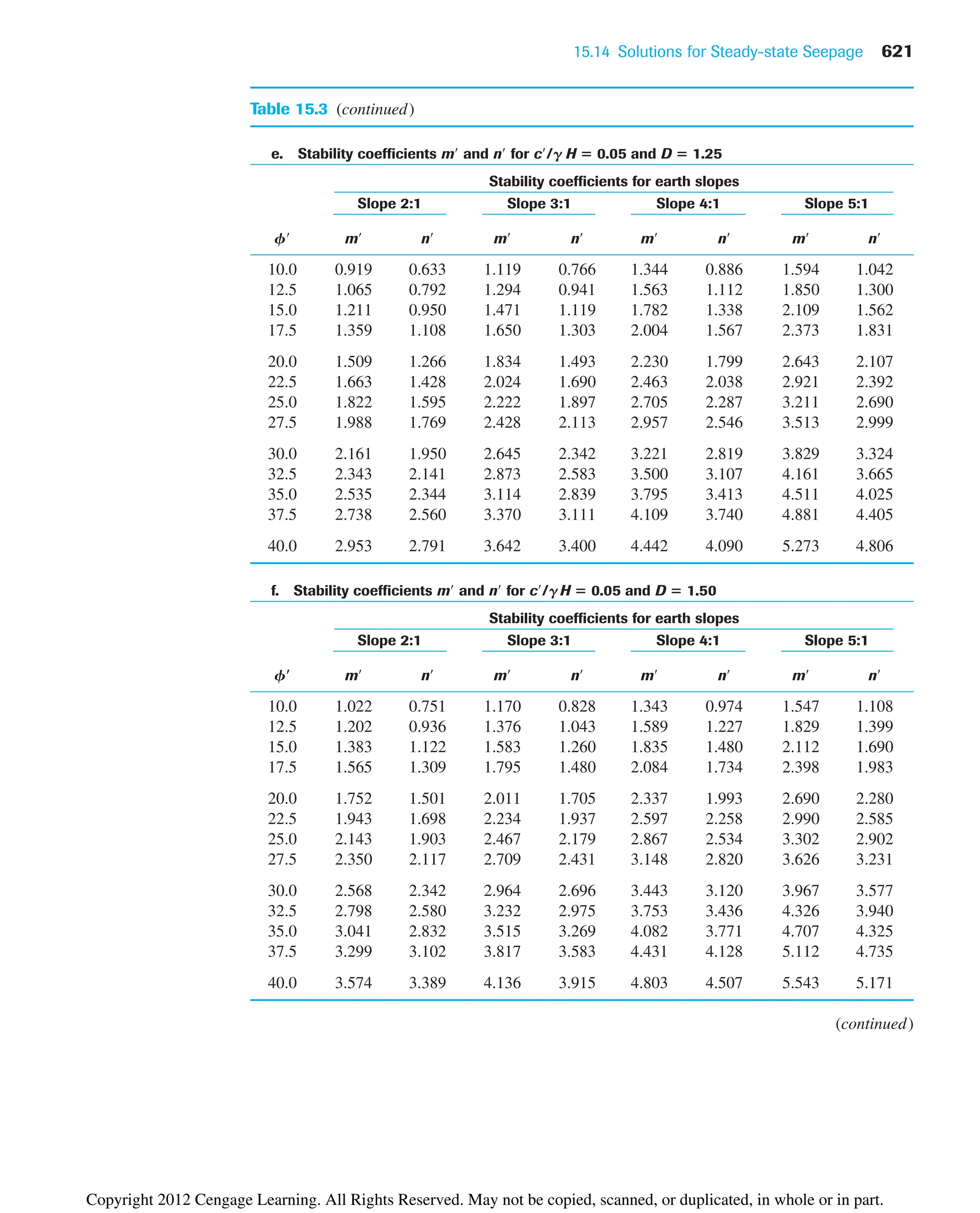
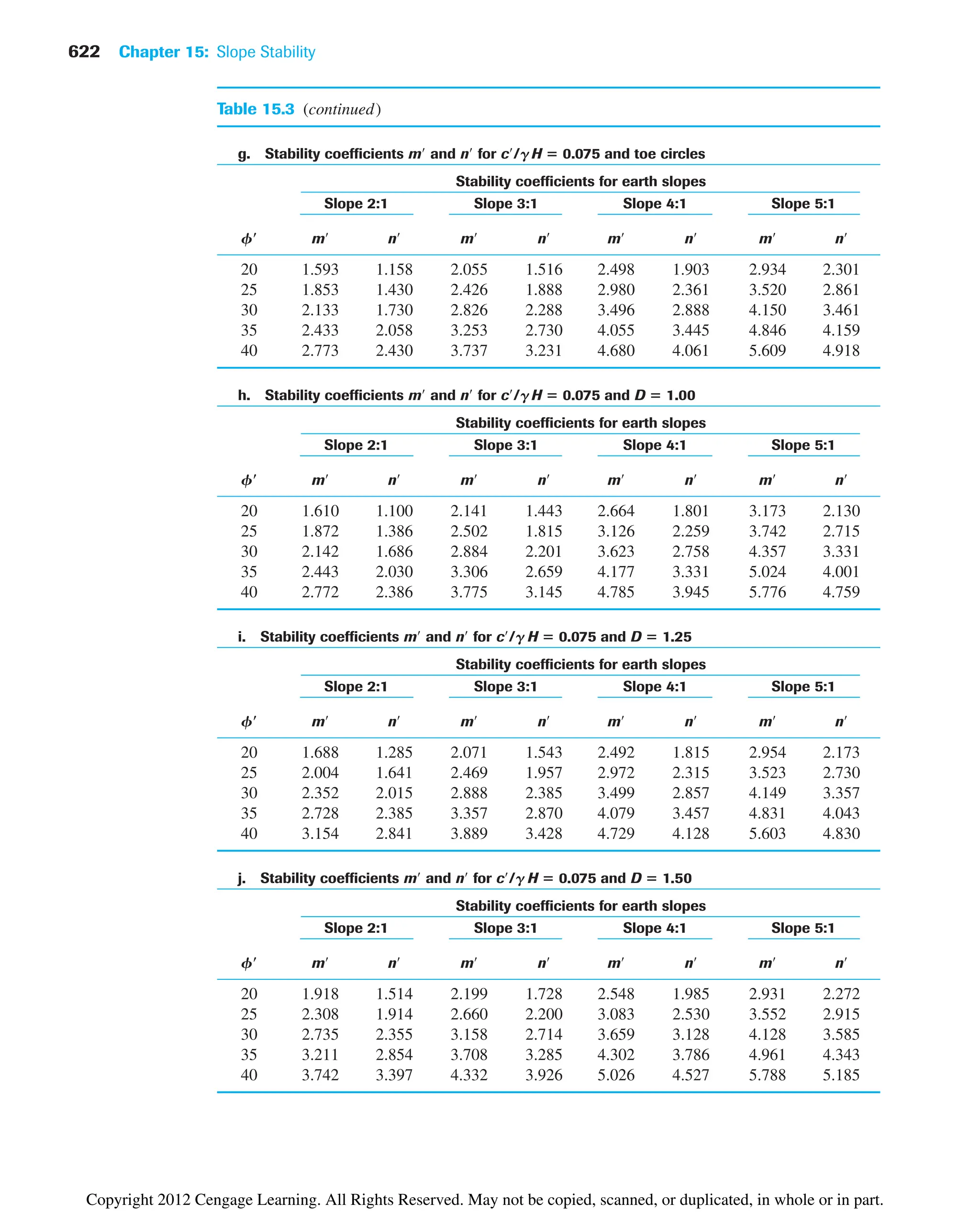
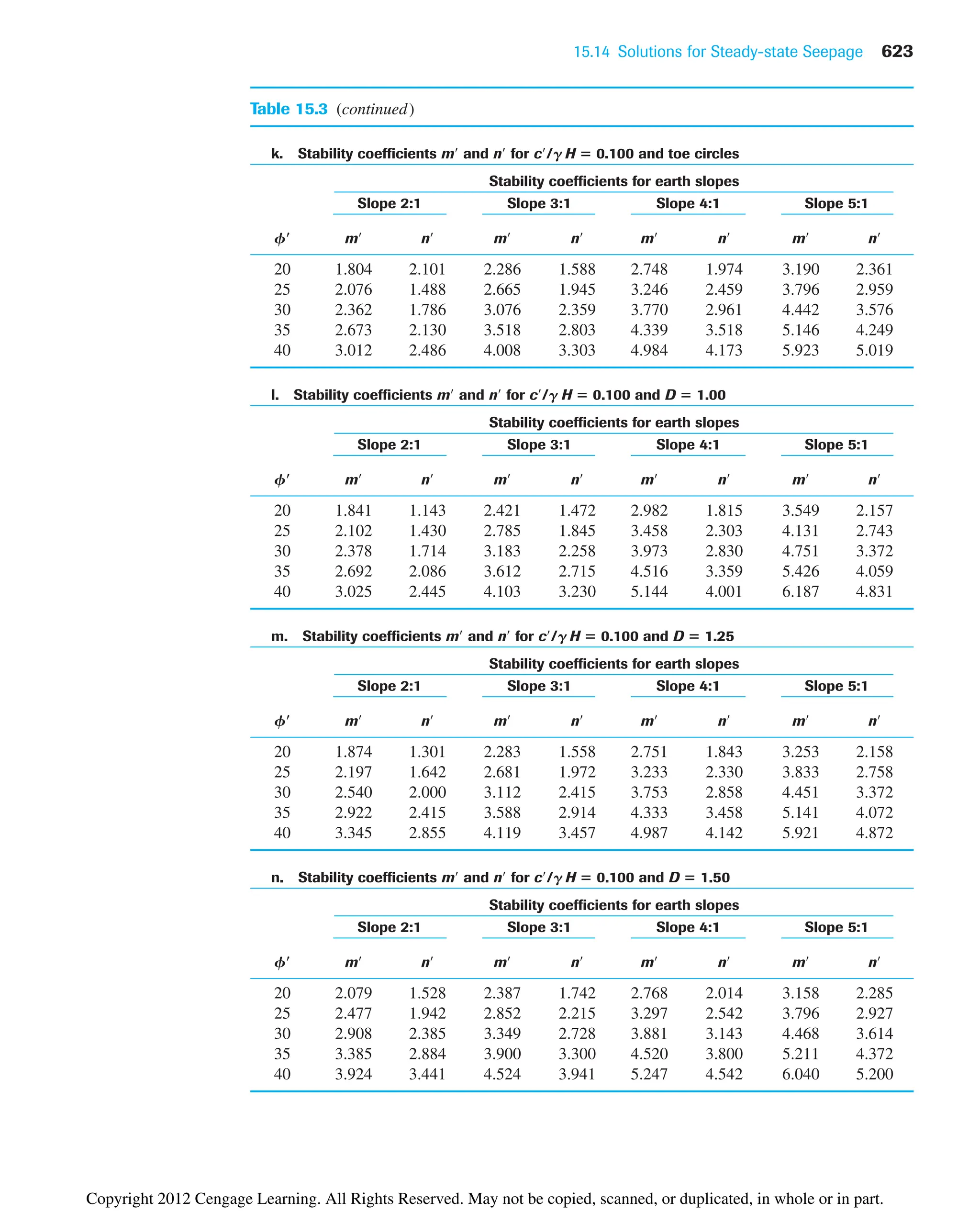
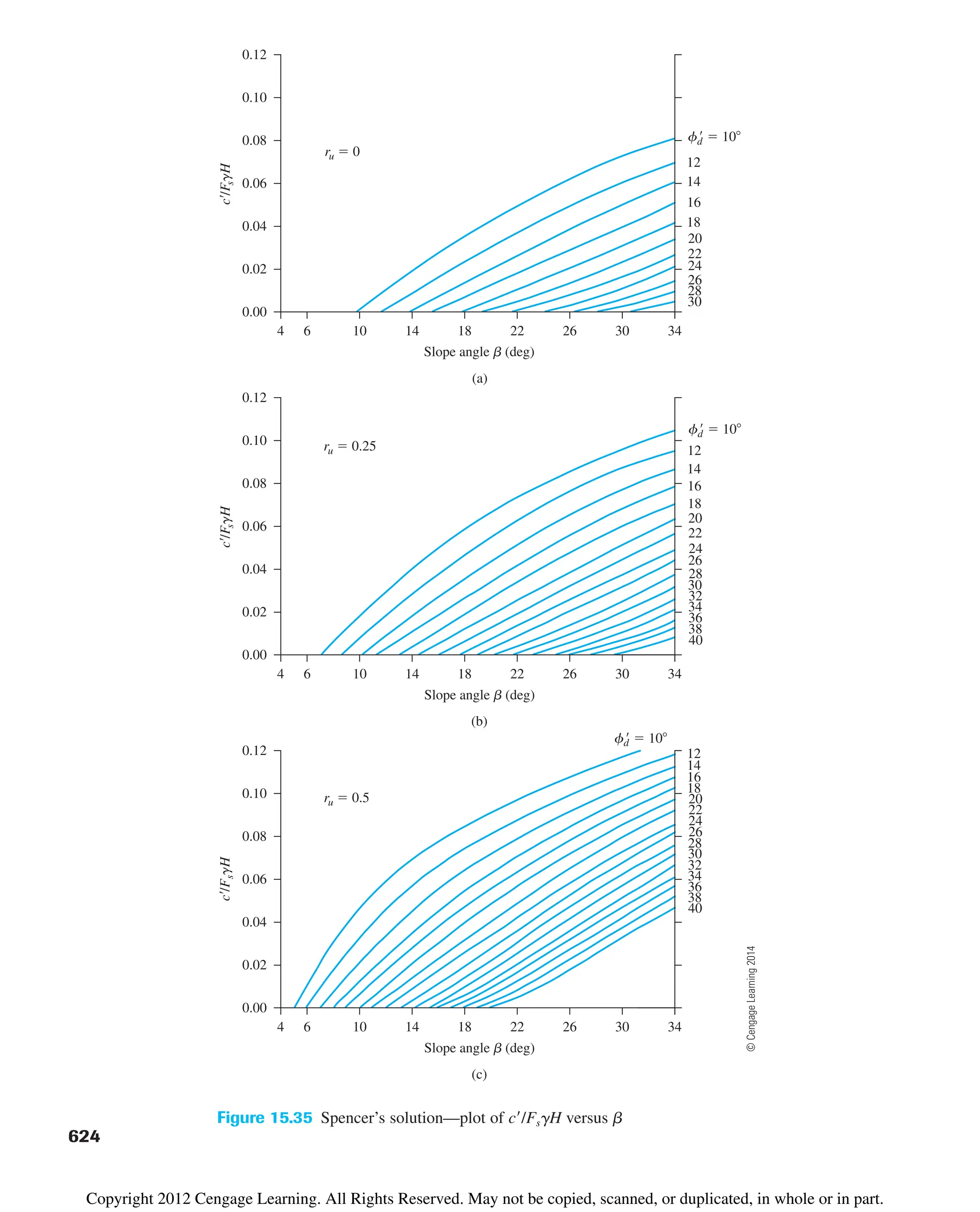
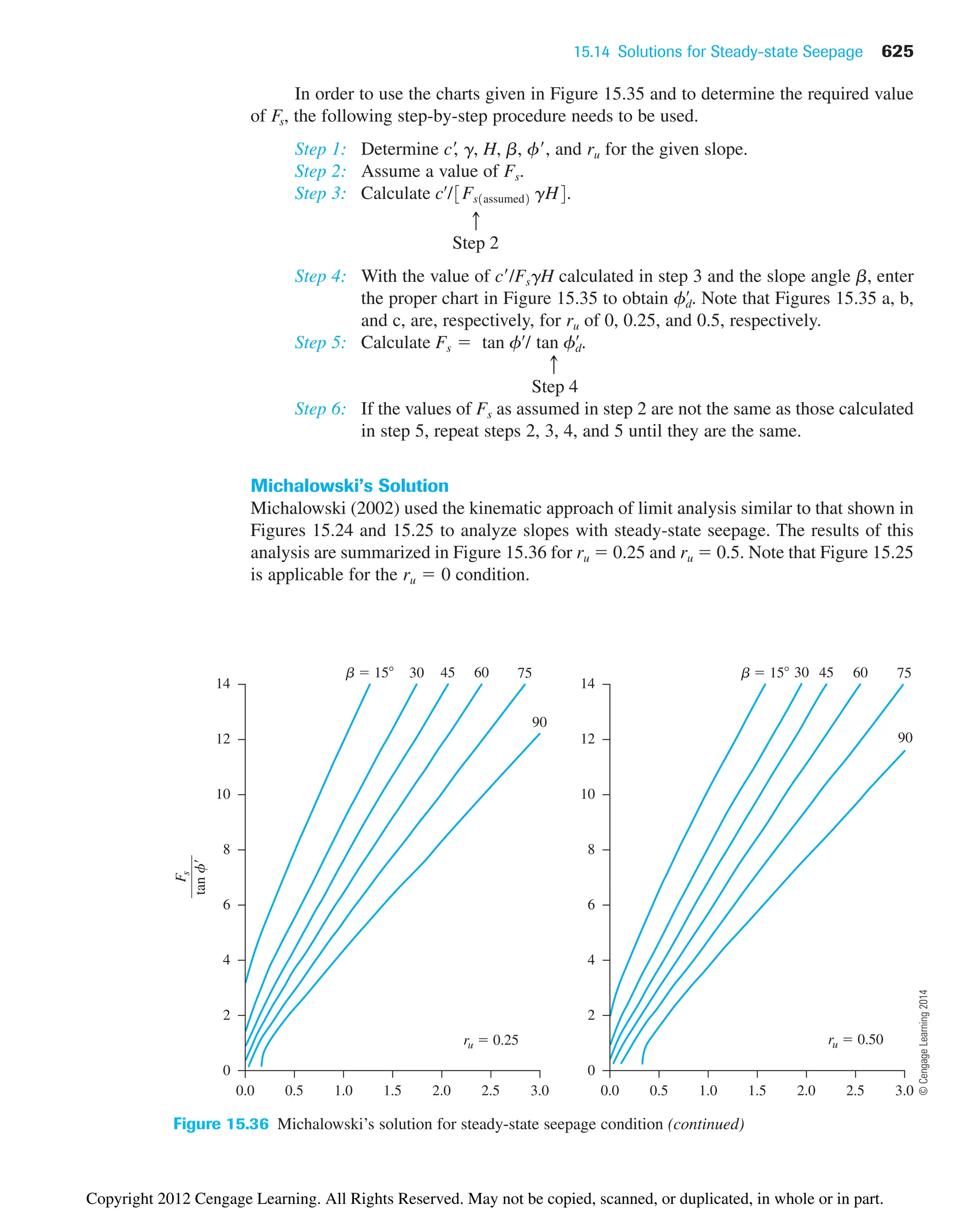
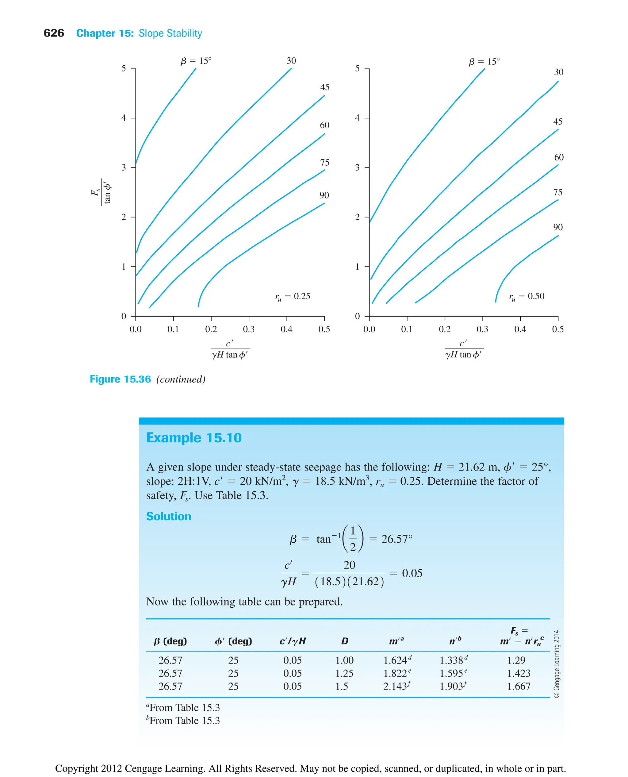
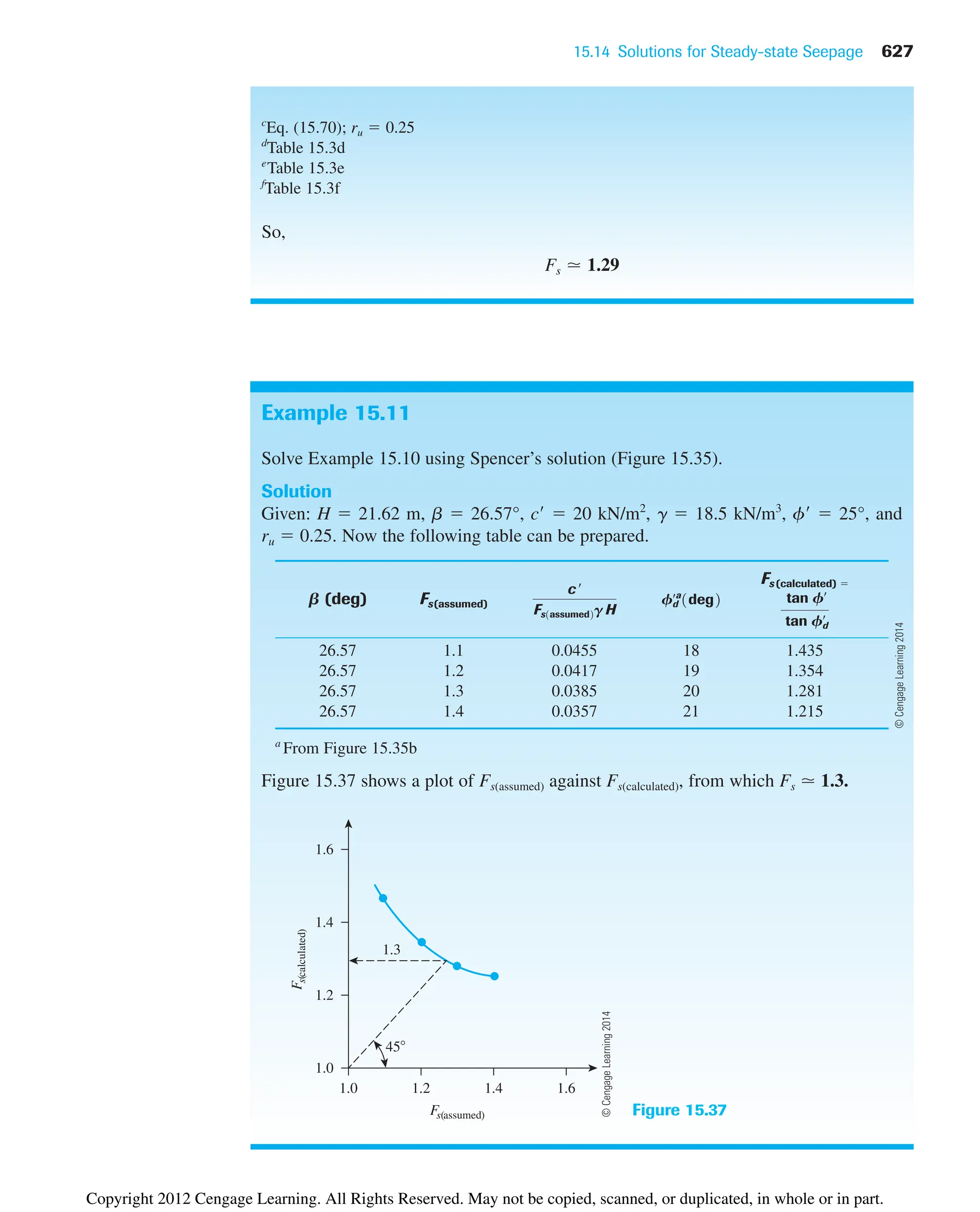
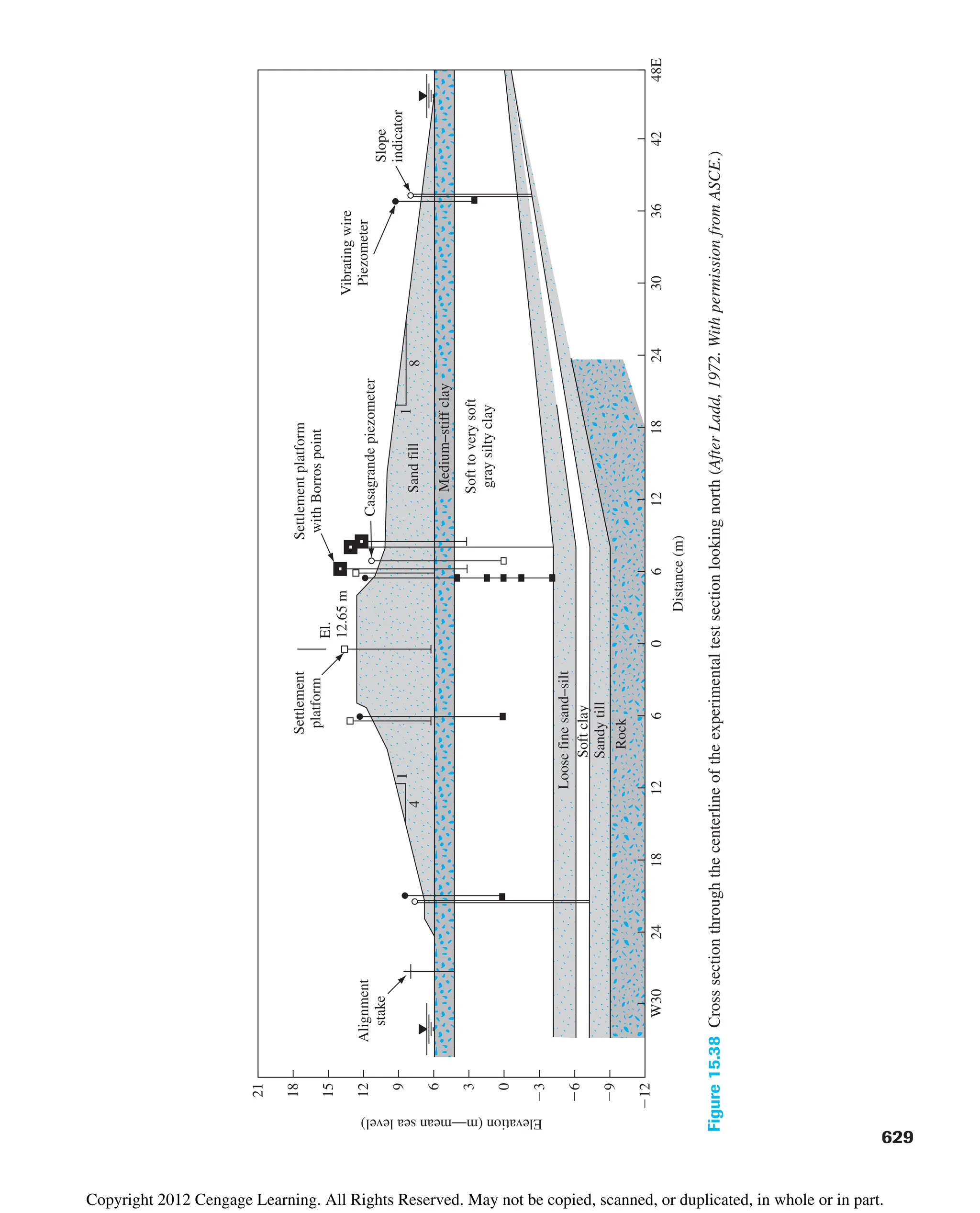
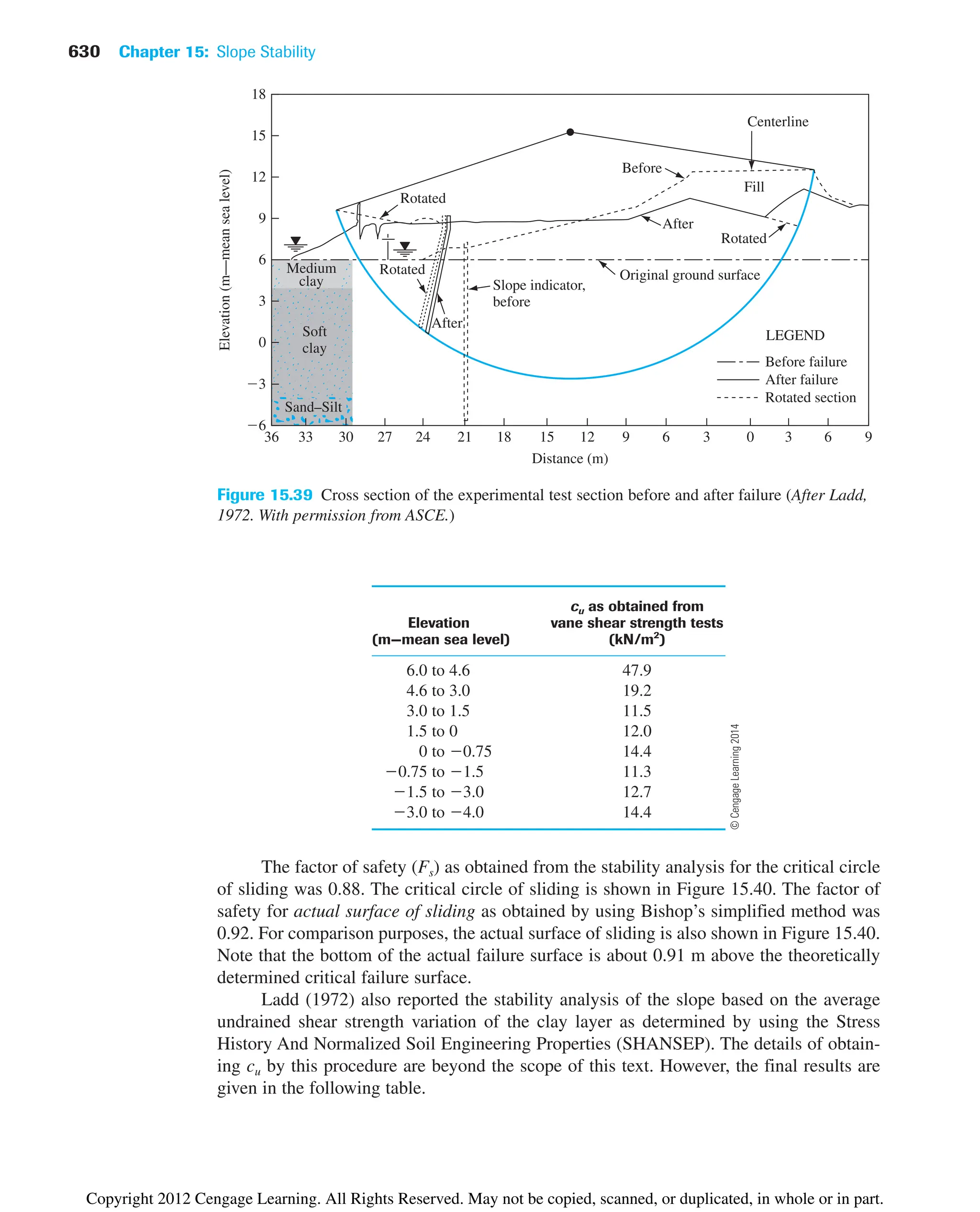
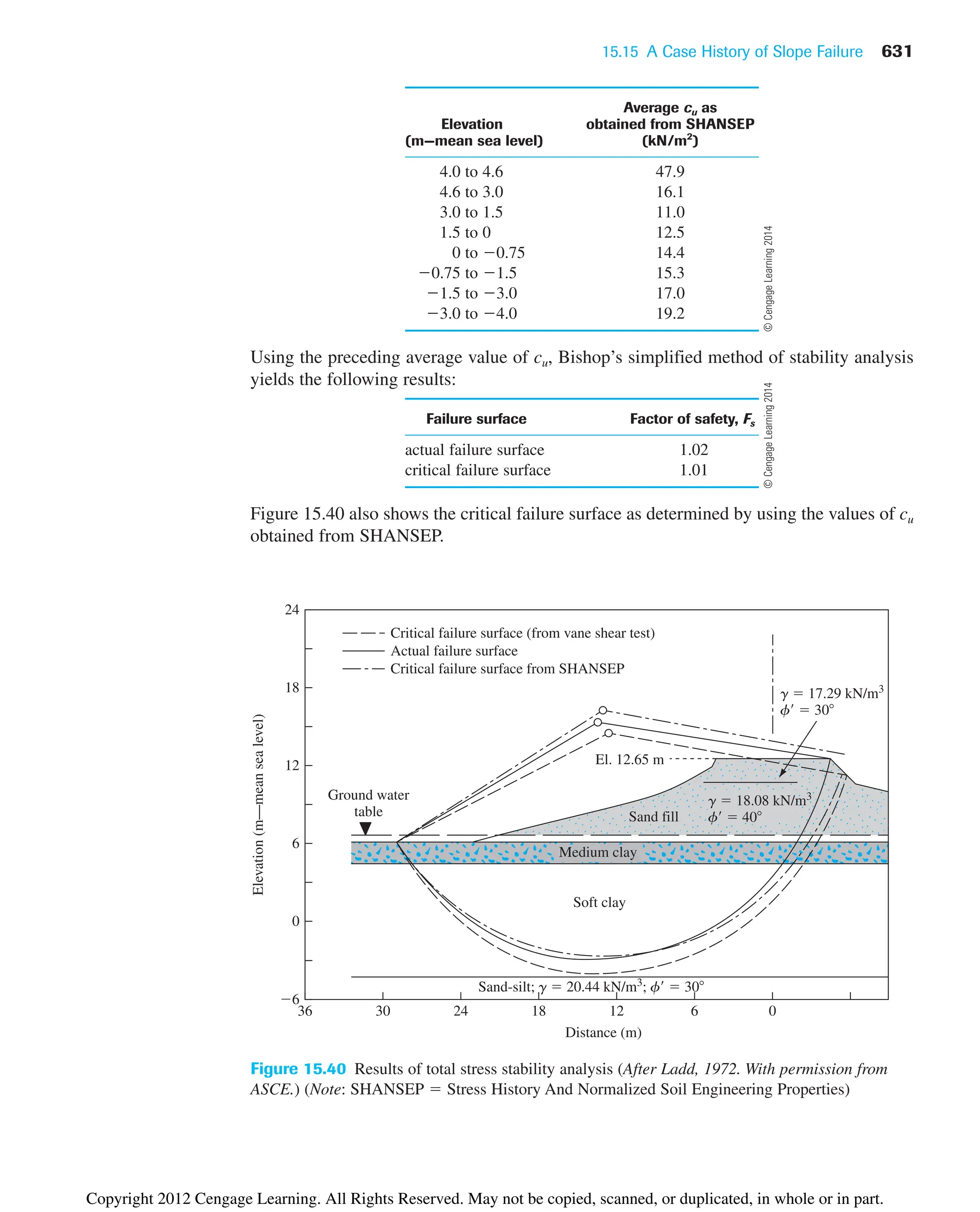
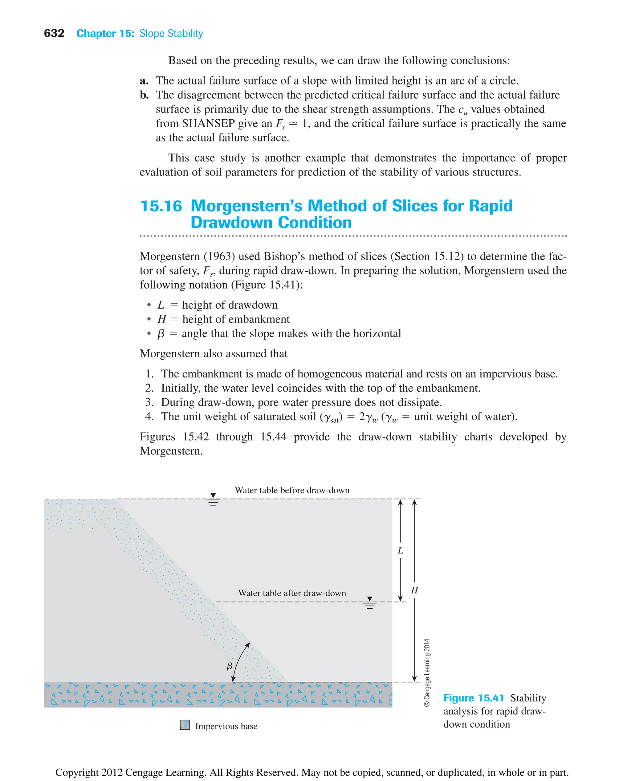
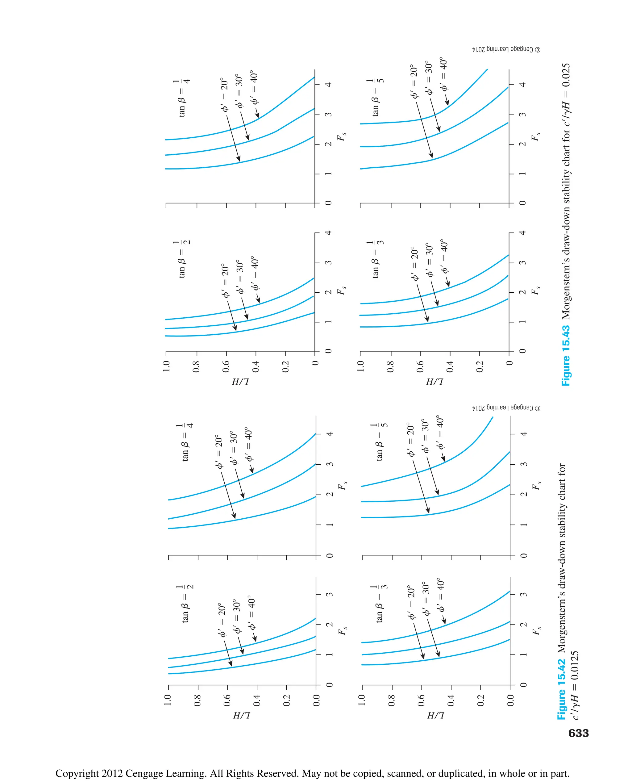

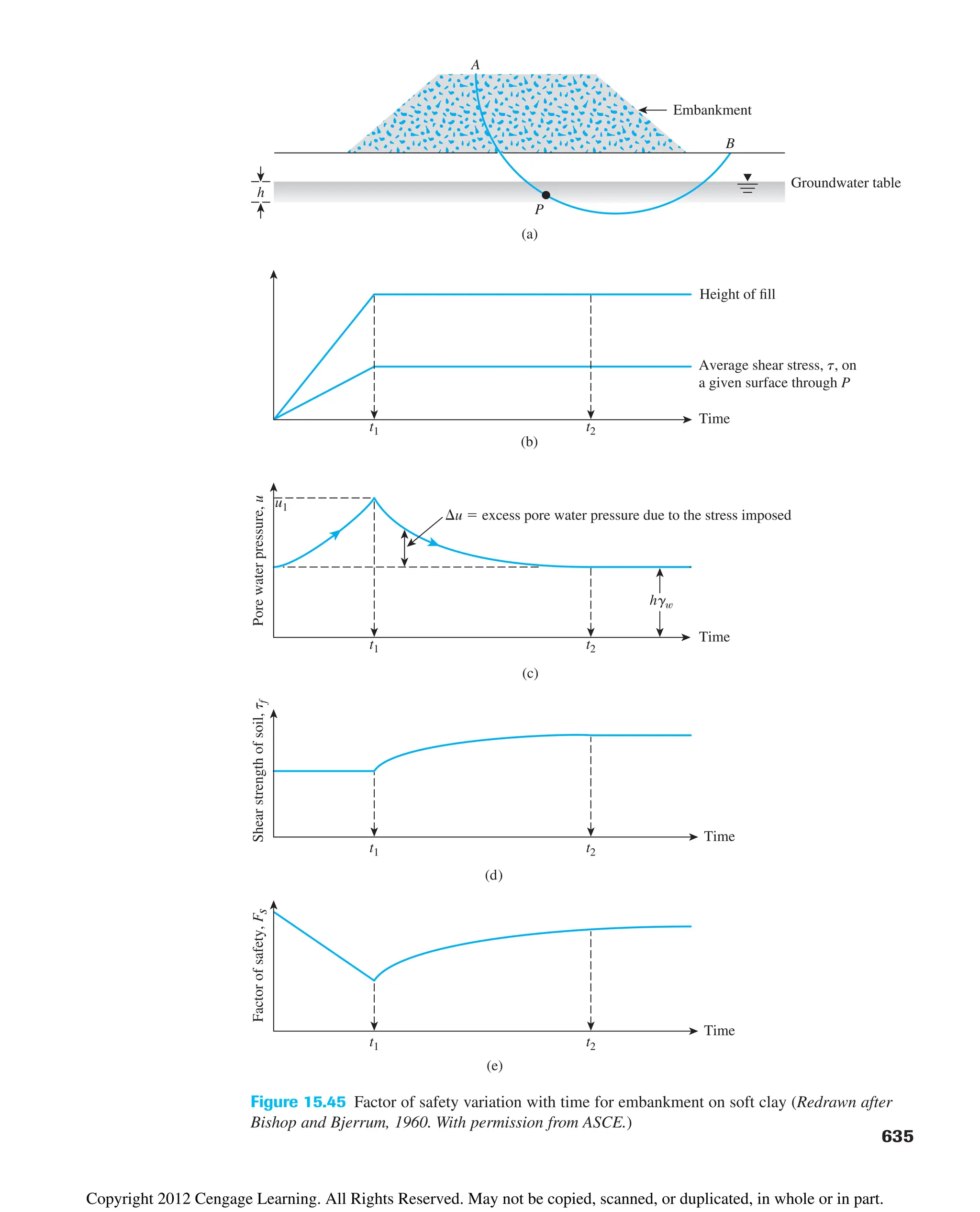
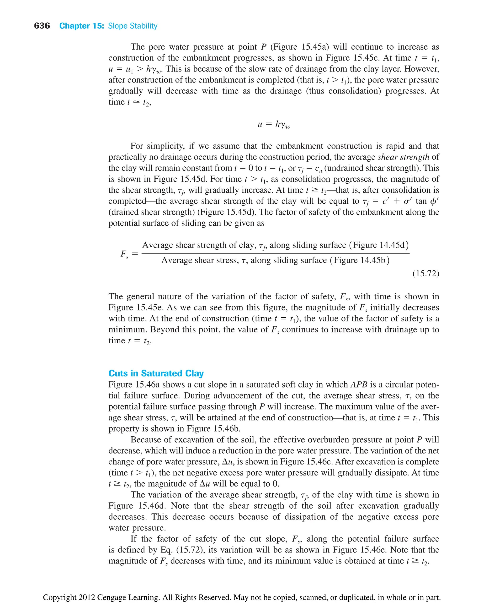
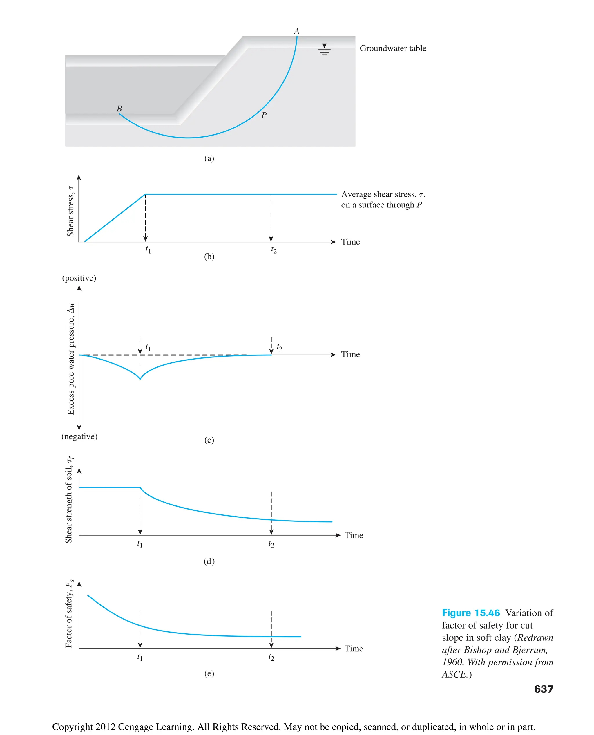
![15.18 Summary
Following is a summary of the topics covered in this chapter:
• The factor of safety with respect to strength (Fs) occurs when [Eq. (15.7)]
• The factors of safety against sliding for infinite slopes for cases with and without
seepage are given by Eqs. (15.15) and (15.28), respectively.
• The critical height of a finite slope with plane failure surface assumption can be
given by Eq. (15.42).
• The modes of failure of finite slopes with circular failure surfaces can be categorized
under (Section 15.7)
• Slope failure
• Base failure
• Stability analysis charts for clay slopes (f 0 condition) are provided in Figures 15.13
and 15.19.
• Stability analysis charts for slopes with cf soil (pore water pressure equal to
zero) are given in Figures 15.21, 15.23, 15.25, and 15.27.
• Determination of factor of safety with respect to strength using the method of slices
with and without seepage is described in Sections 15.11 and 15.12.
• Stability analysis of slopes with circular failure surface under steady-state seepage is
presented in Sections 15.13 and 15.14.
Fs Fcœ Ffœ
638 Chapter 15: Slope Stability
Problems
15.1 Refer to the infinite slope shown in Figure 15.47. Given: b 25°, g
17.8 kN/m3
, f 28°, and c 31 kN/m2
. Find the height, H, such that a factor
of safety, Fs, of 2.75 is maintained against sliding along the soil–rock interface.
H
b
g
f
c
b
Rock
Figure 15.47
©
Cengage
Learning
2014
Copyright 2012 Cengage Learning. All Rights Reserved. May not be copied, scanned, or duplicated, in whole or in part.](https://image.slidesharecdn.com/principlesofgeotechnicalengineering-8thedition-231222125509-7e44d9bf/75/Principles-of-Geotechnical-Engineering-8th-Edition-pdf-658-2048.jpg)
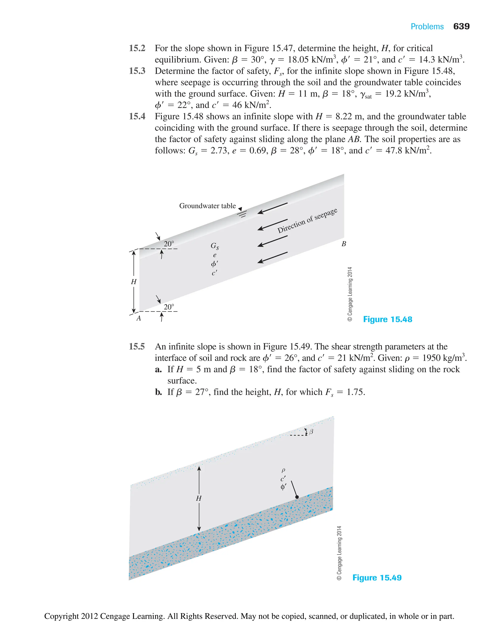
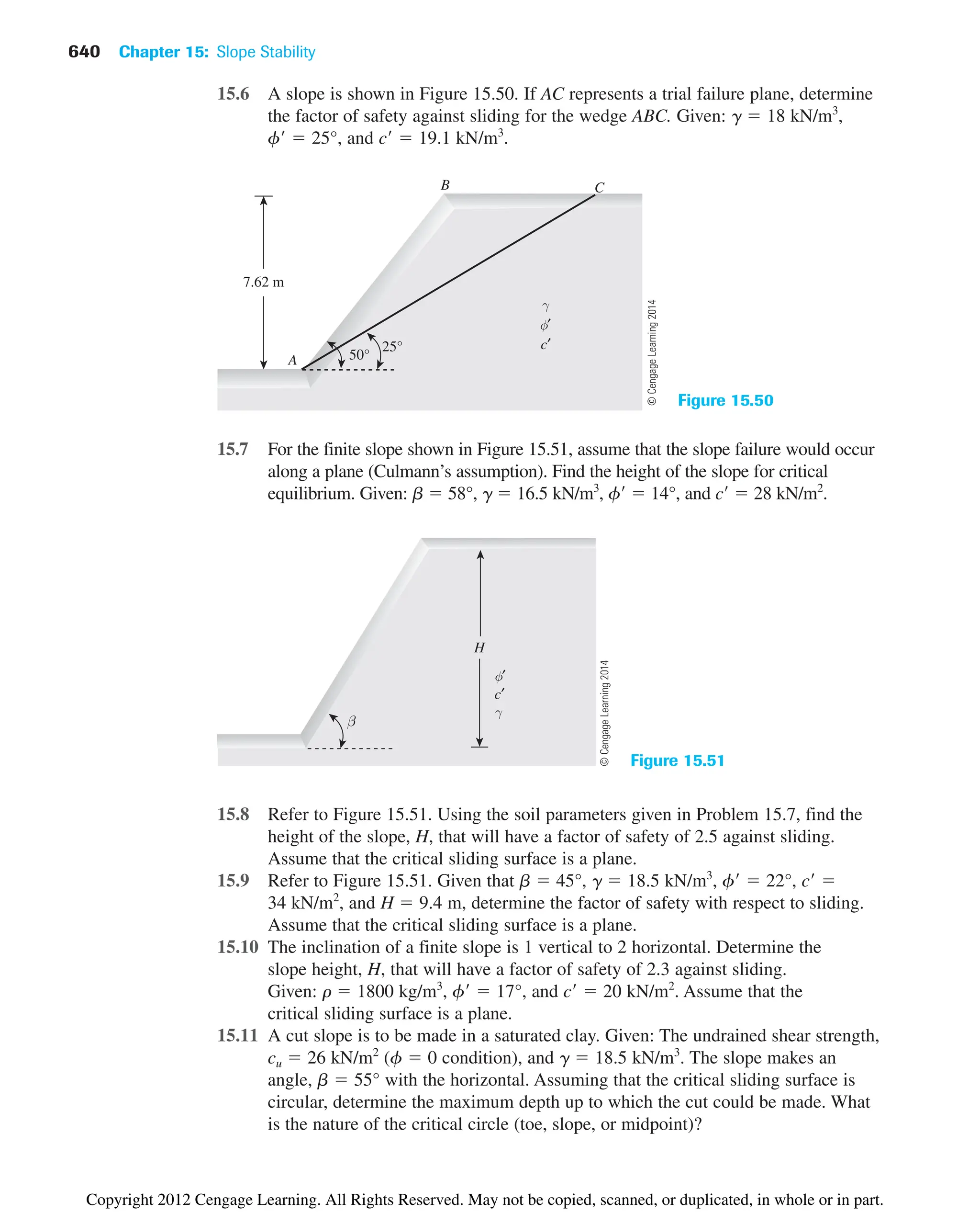
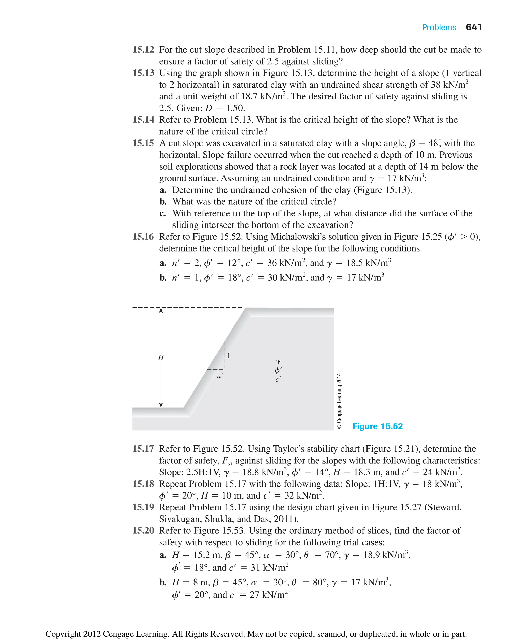
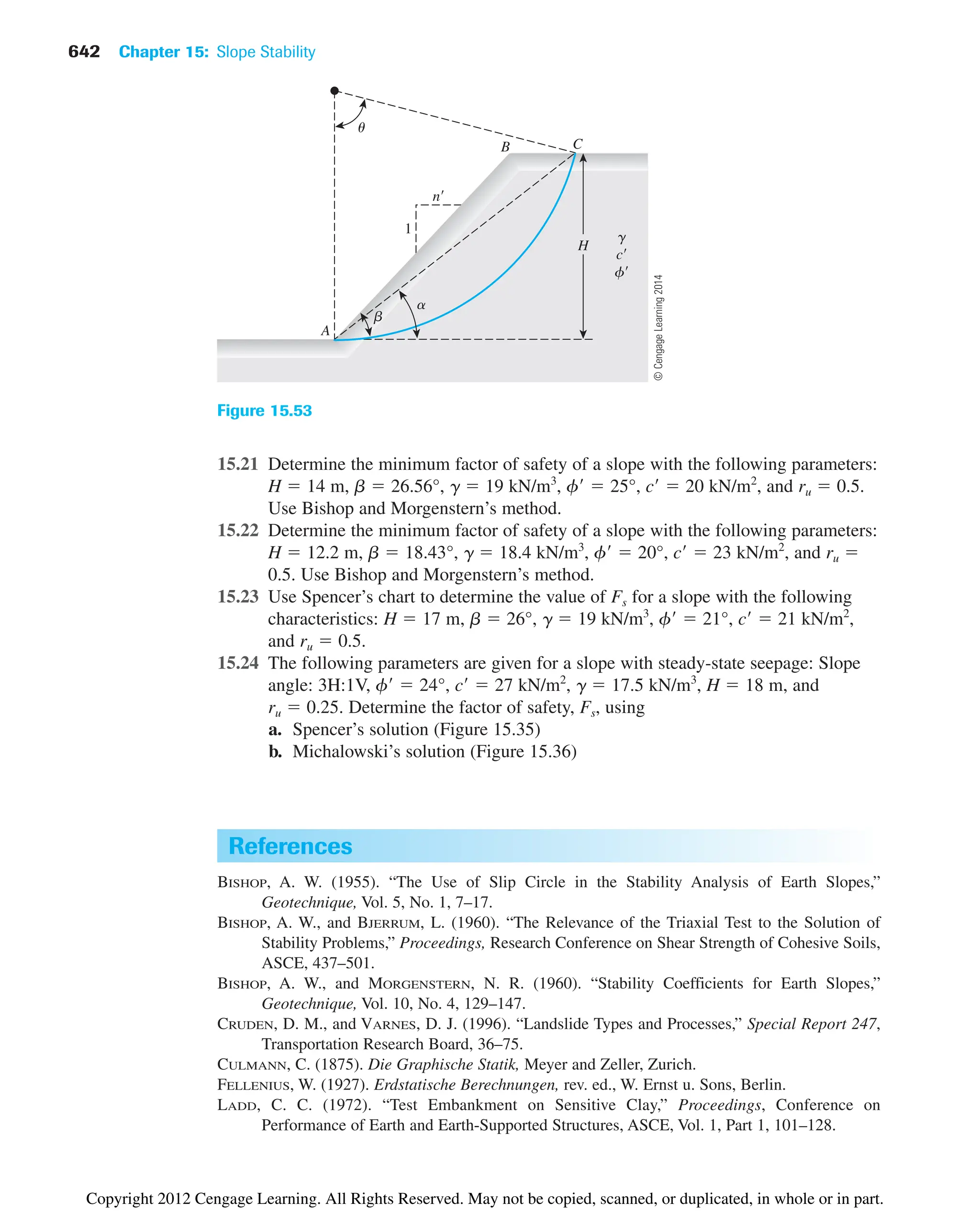

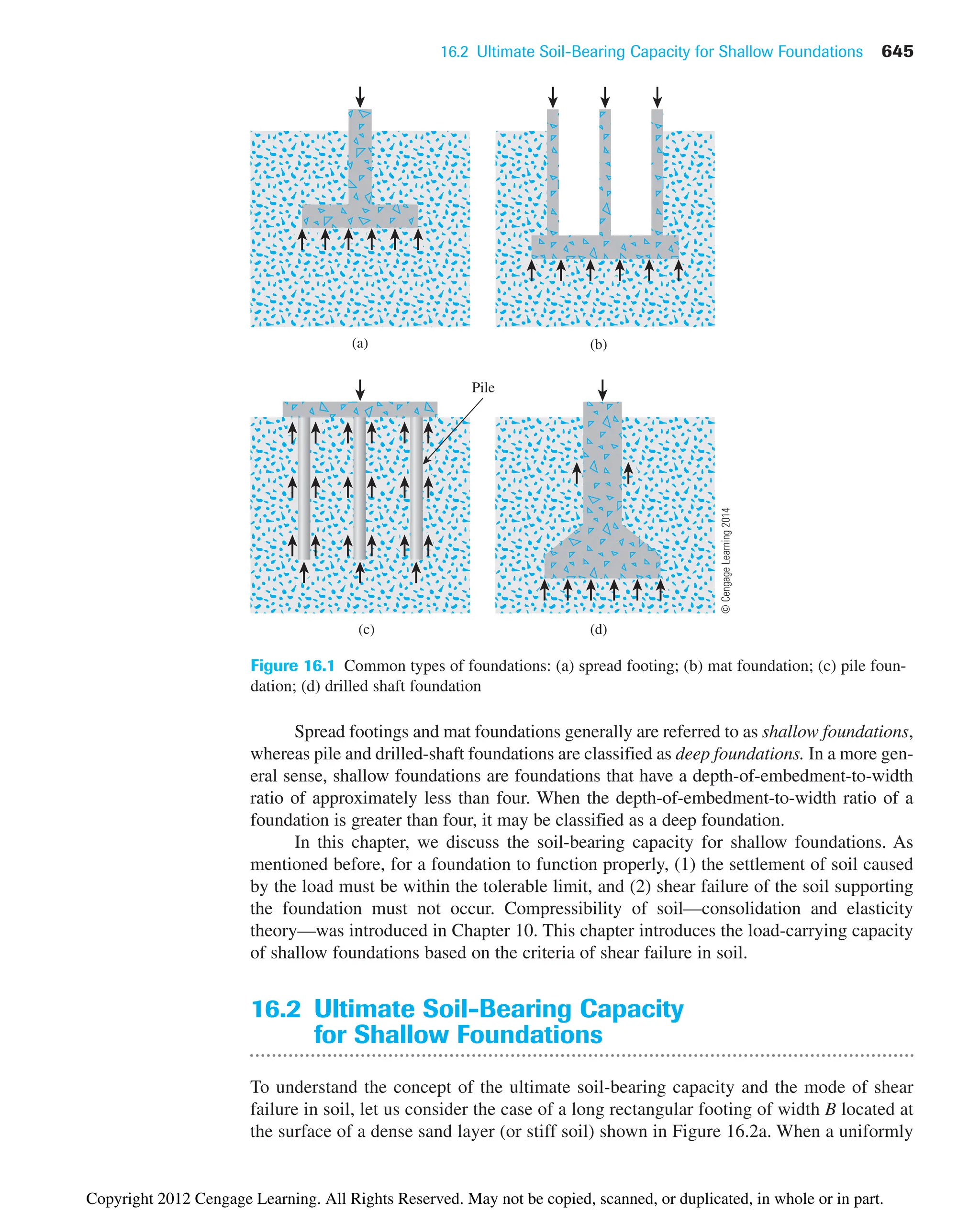
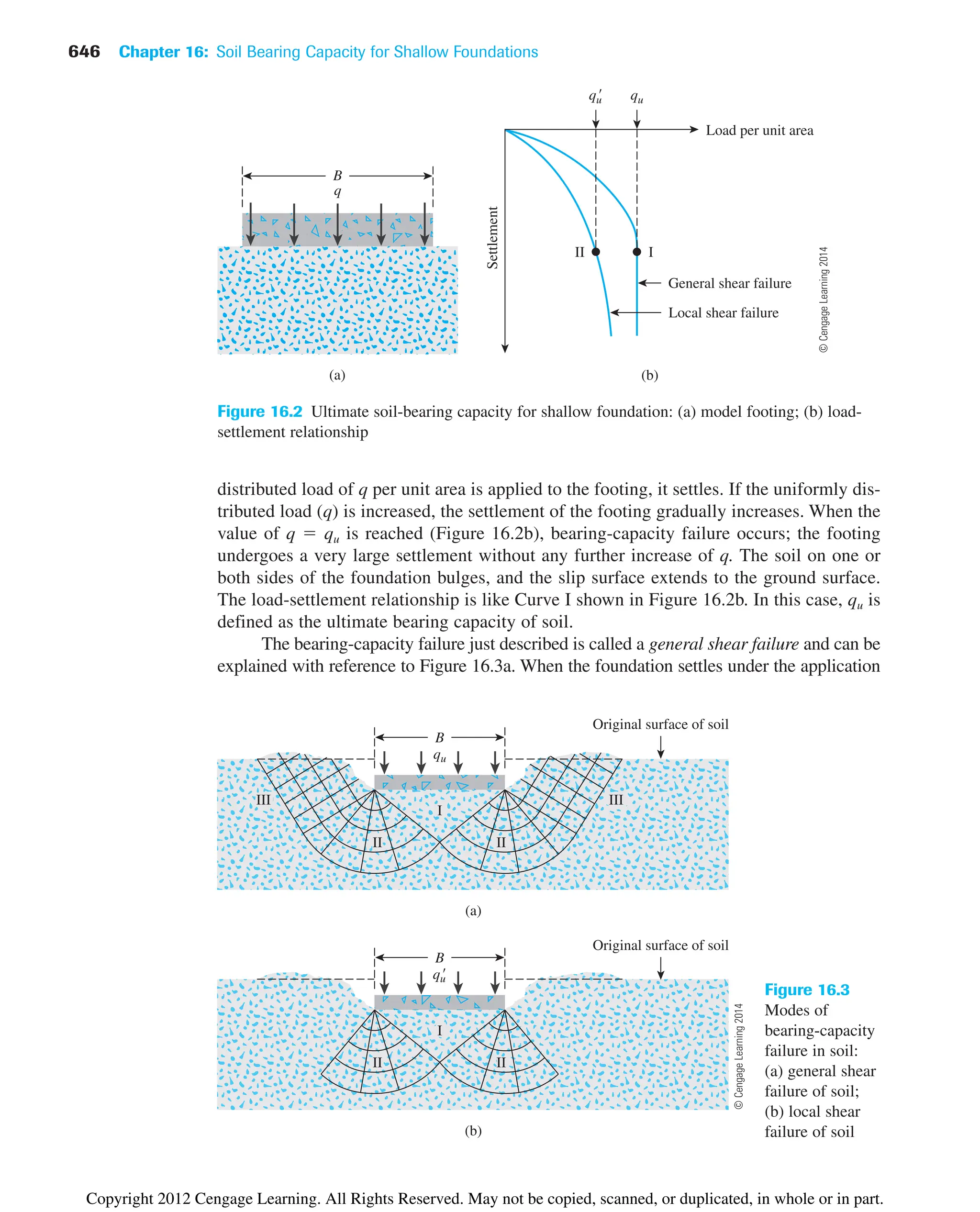
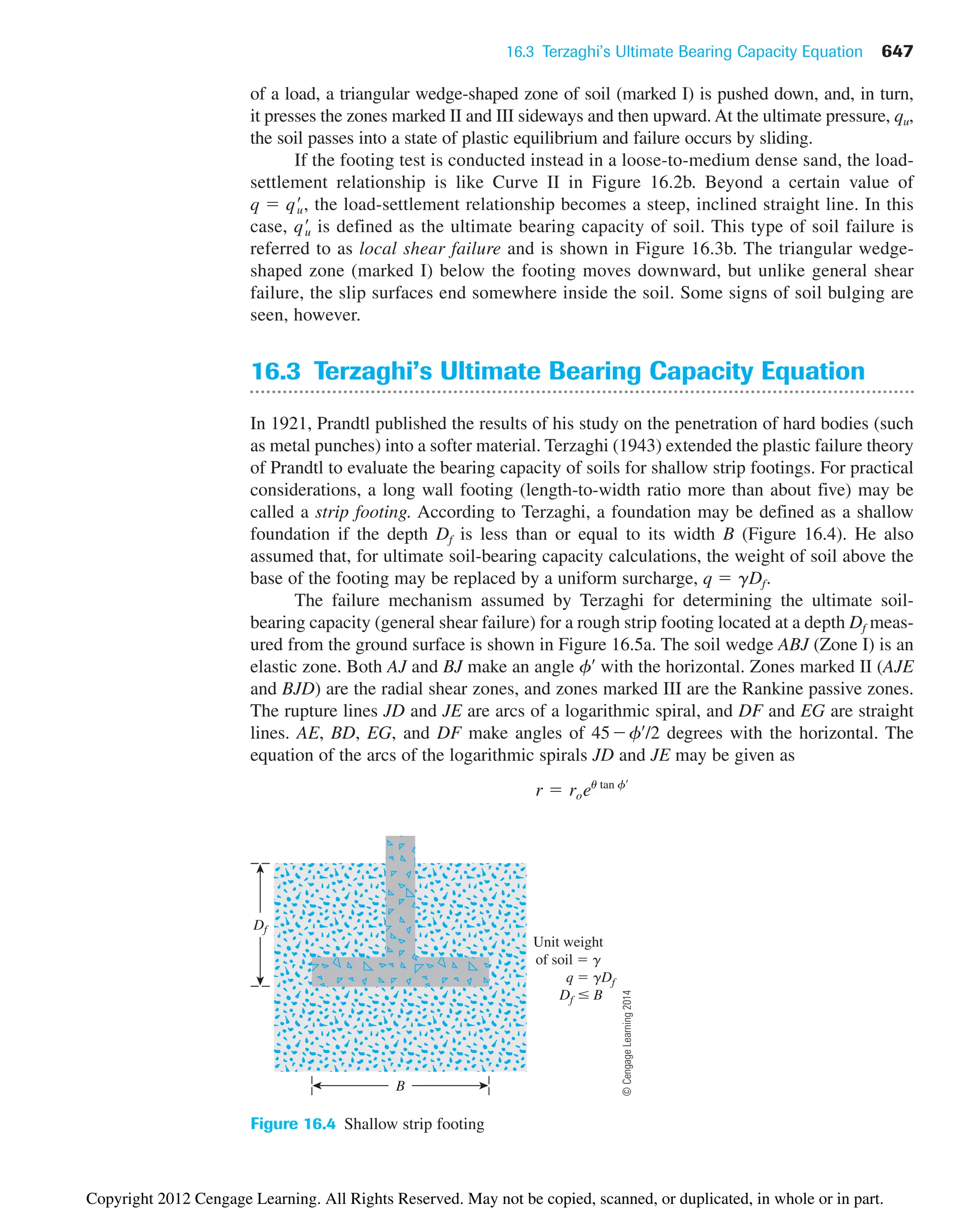
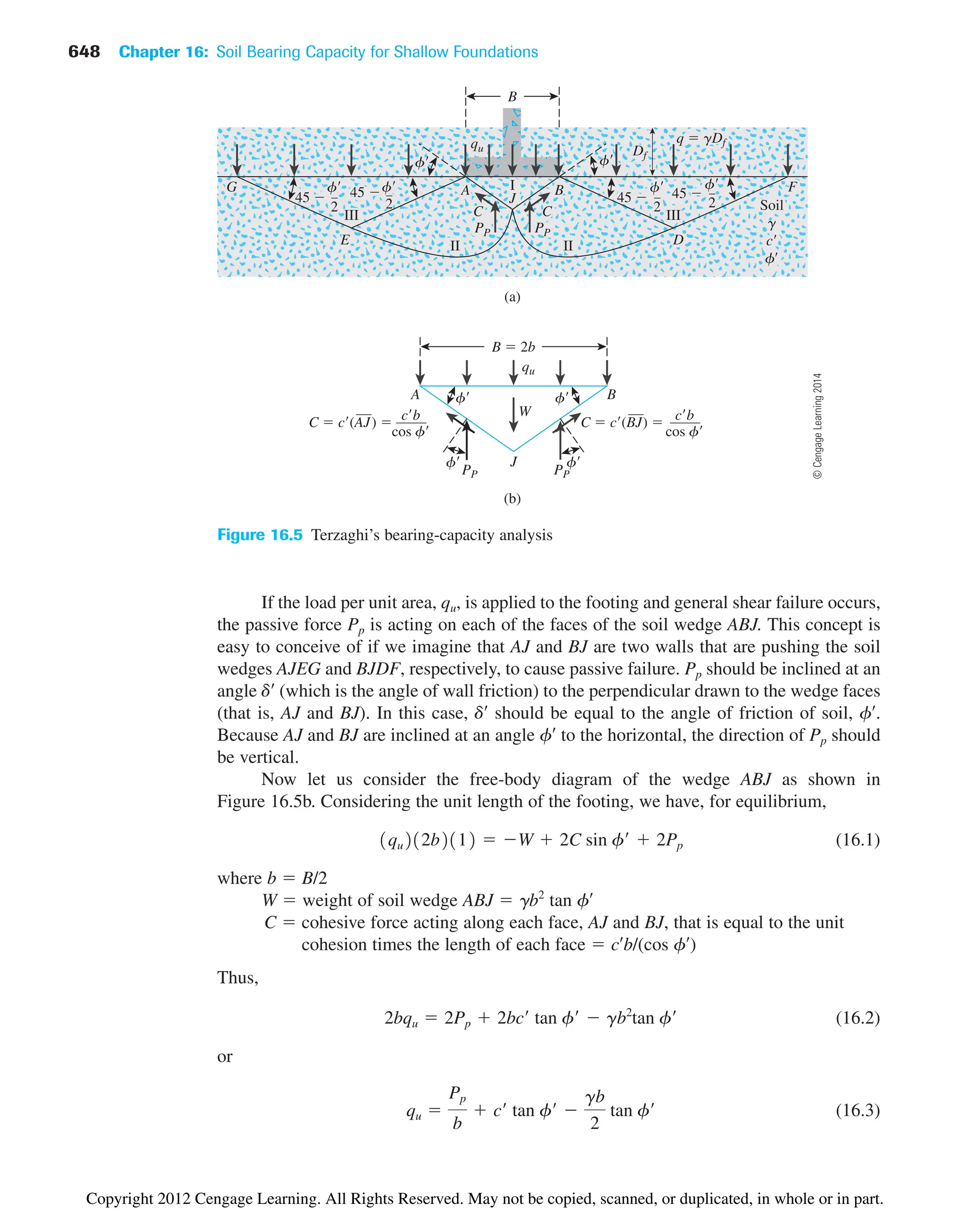
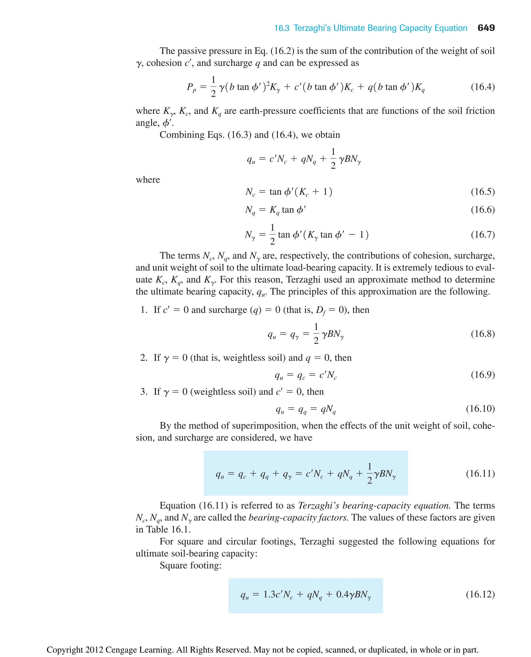
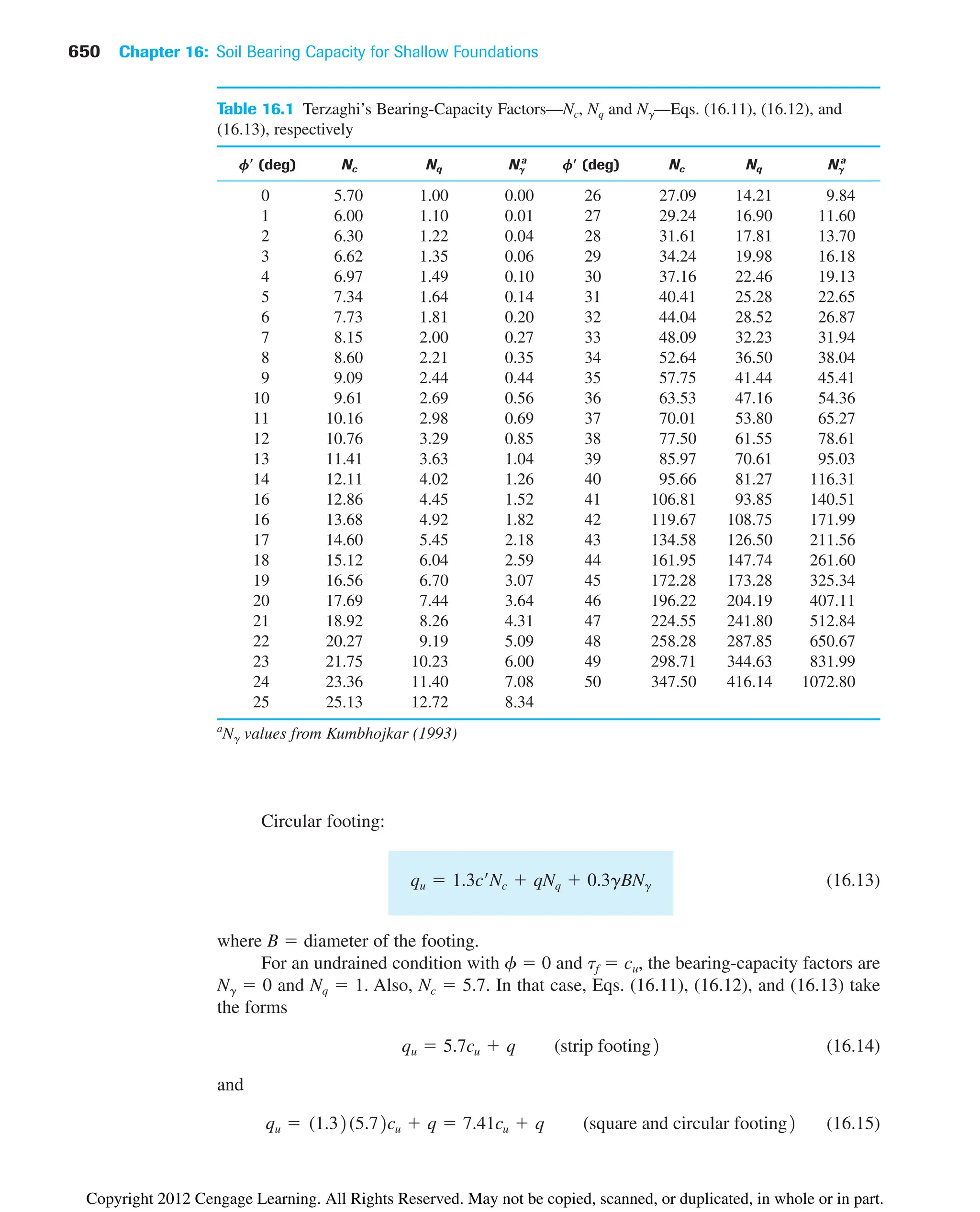
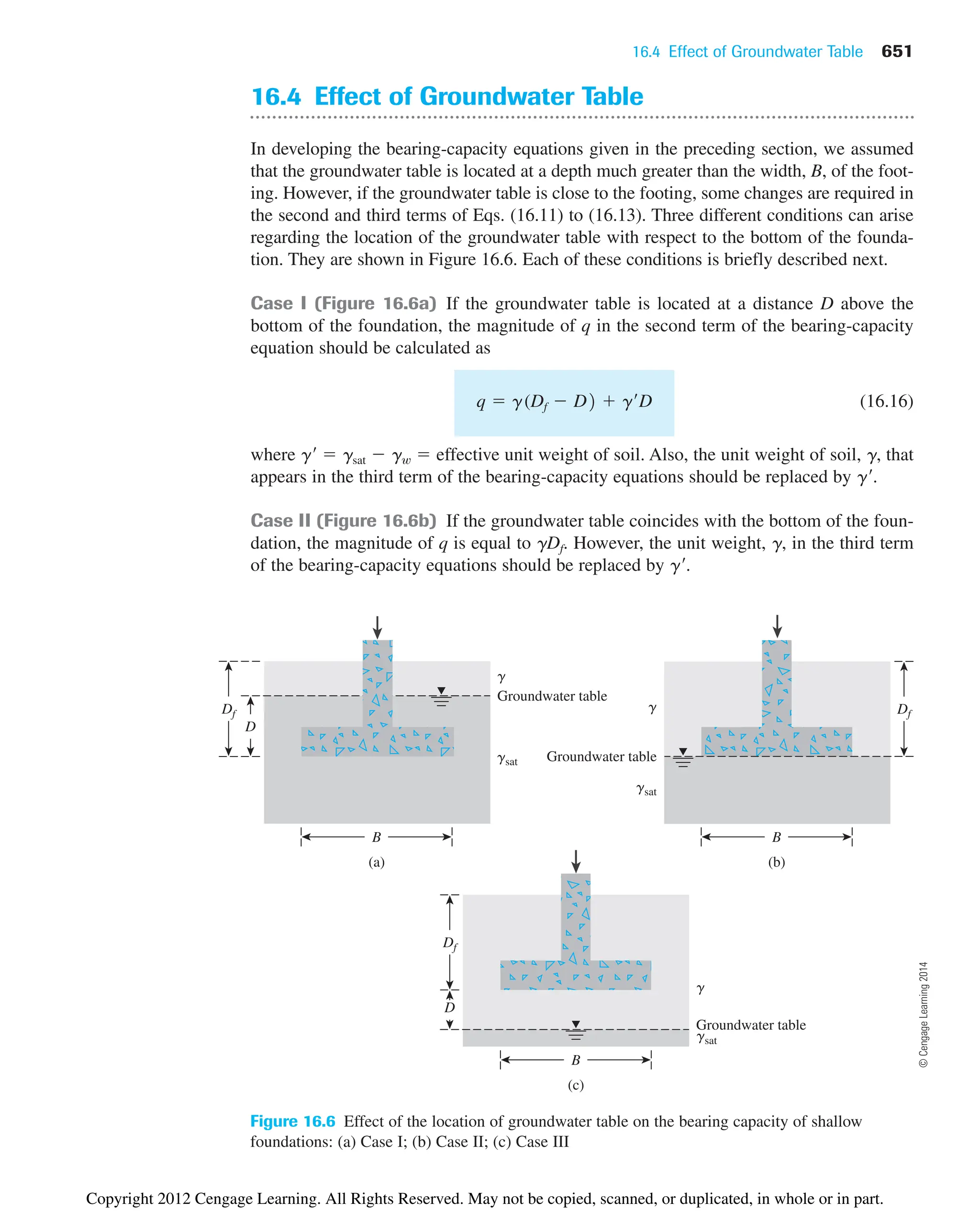
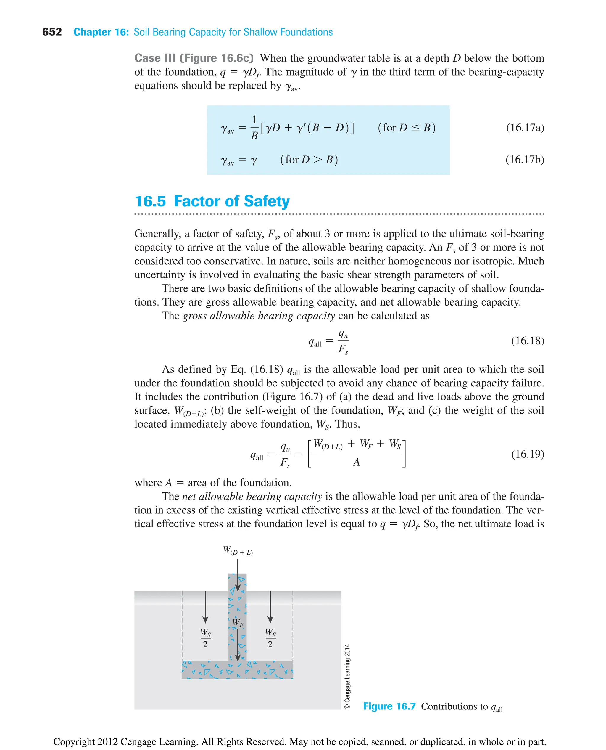
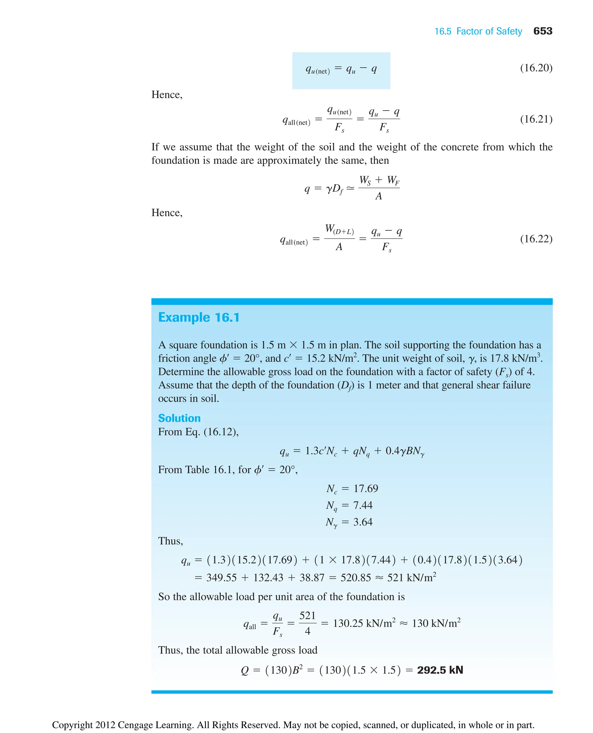
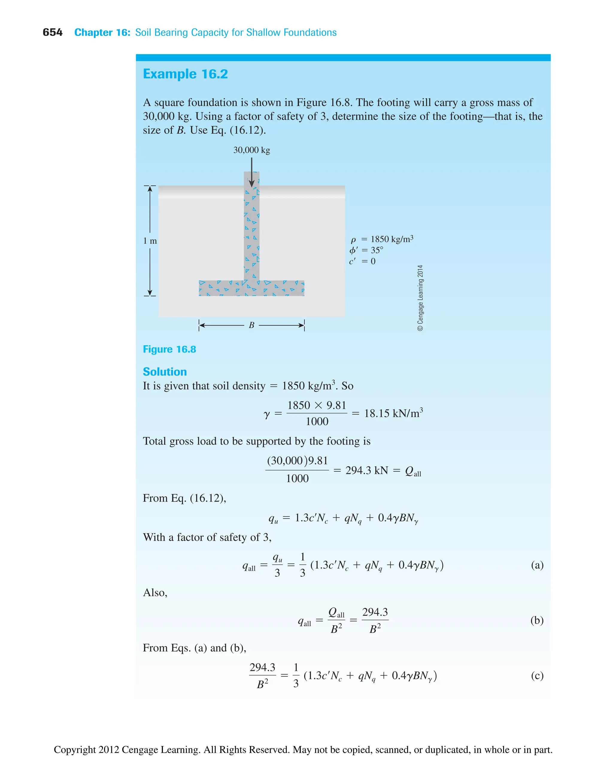
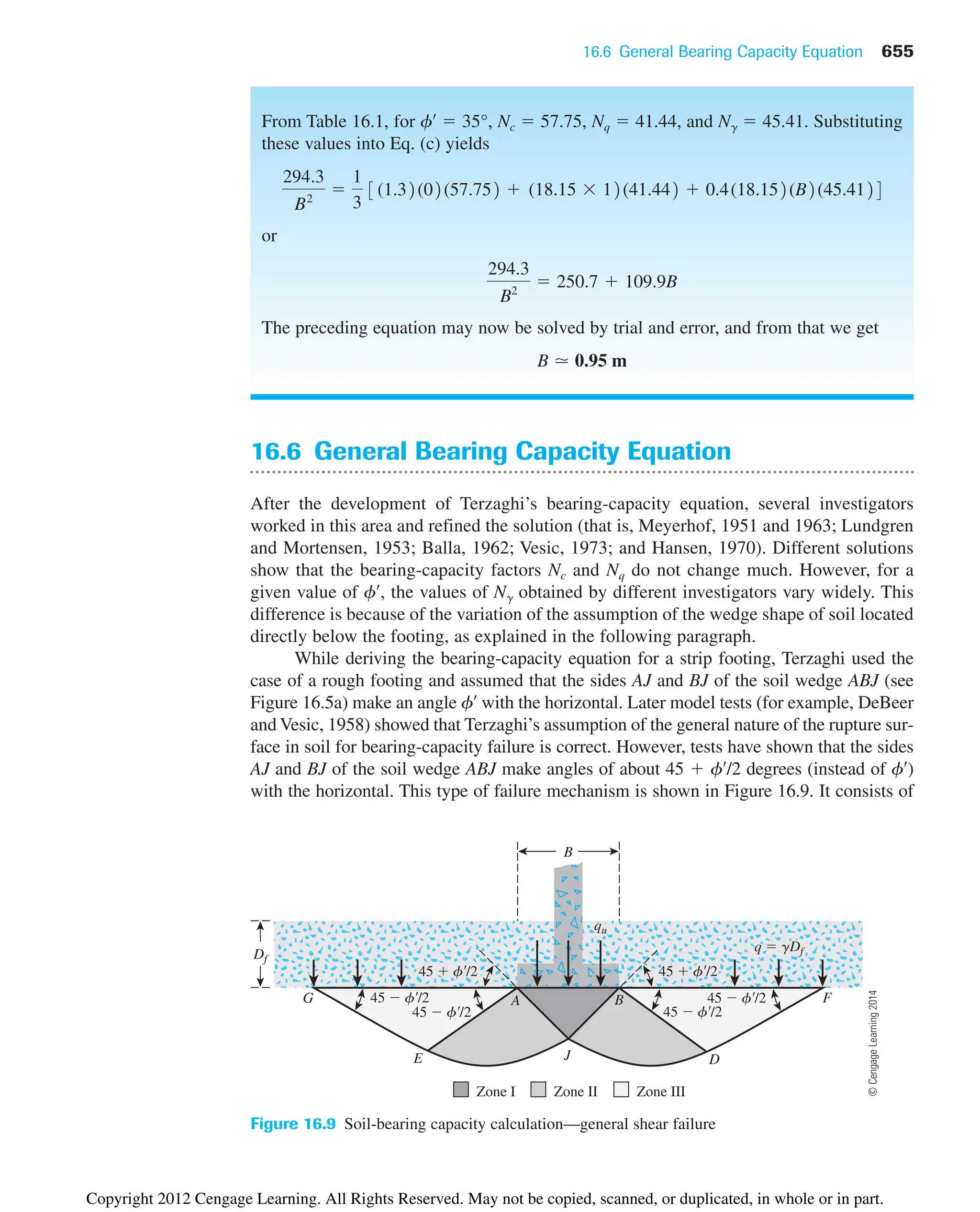
![a Rankine active zone ABJ (Zone I), two radial shear zones (Zones II), and two Rankine
passive zones (Zones III). The curves JD and JE are arcs of a logarithmic spiral.
On the basis of this type of failure mechanism, the ultimate bearing capacity of a
strip footing may be evaluated by the approximate method of superimposition described in
Section 16.3 as
(16.23)
where qc, qq, and q␥ are the contributions of cohesion, surcharge, and unit weight of soil,
respectively.
Reissner (1924) expressed qq as
(16.24)
where
(16.25)
Prandtl (1921) showed that
(16.26)
where
(16.27)
Vesic (1973) expressed q␥ as
(16.28)
where
(16.29)
Combining Eqs. (16.23), (16.24), (16.26), and (16.28), we obtain
(16.30)
This equation is in the same general form as that given by Terzaghi [Eq. (16.11)]; however,
the values of the bearing capacity factors are not the same. The values of Nq, Nc, and N␥,
defined by Eqs. (16.25), (16.27), and (16.29), are given in Table 16.2. But for all practical
purposes, Terzaghi’s bearing-capacity factors will yield good results. Differences in
bearing-capacity factors are usually minor compared with the unknown soil parameters.
qu c¿Nc qNq
1
2
gBNg
Eq. 116.252
c
Ng 21Nq 12 tan fœ
qg
1
2
BgNg
Eq. 116.252
c
Nc (Nq 12cot f¿
qc c¿Nc
Nq ep tan f¿
tan2
a45
f¿
2
b
qq qNq
qu qc qq qg
656 Chapter 16: Soil Bearing Capacity for Shallow Foundations
Copyright 2012 Cengage Learning. All Rights Reserved. May not be copied, scanned, or duplicated, in whole or in part.](https://image.slidesharecdn.com/principlesofgeotechnicalengineering-8thedition-231222125509-7e44d9bf/75/Principles-of-Geotechnical-Engineering-8th-Edition-pdf-676-2048.jpg)
![16.6 General Bearing Capacity Equation 657
Table 16.2 Bearing-Capacity Factors Nc, Nq, and N␥ [Eqs. (16.25), (16.27) and (16.29)]
ⴕ (deg) Nc Nq N␥ ⴕ (deg) Nc Nq N␥
0 5.14 1.00 0.00 26 22.25 11.85 12.54
1 5.38 1.09 0.07 27 23.94 13.20 14.47
2 5.63 1.20 0.15 28 25.80 14.72 16.72
3 5.90 1.31 0.24 29 27.86 16.44 19.34
4 6.19 1.43 0.34 30 30.14 18.40 22.40
5 6.49 1.57 0.45 31 32.67 20.63 25.99
6 6.81 1.72 0.57 32 35.49 23.18 30.22
7 7.16 1.88 0.71 33 38.64 26.09 35.19
8 7.53 2.06 0.86 34 42.16 29.44 41.06
9 7.92 2.25 1.03 35 46.12 33.30 48.03
10 8.35 2.47 1.22 36 50.59 37.75 56.31
11 8.80 2.71 1.44 37 55.63 42.92 66.19
12 9.28 2.97 1.69 38 61.35 48.93 78.03
13 9.81 3.26 1.97 39 67.87 55.96 92.25
14 10.37 3.59 2.29 40 75.31 64.20 109.41
15 10.98 3.94 2.65 41 83.86 73.90 130.22
16 11.63 4.34 3.06 42 93.71 85.38 155.55
17 12.34 4.77 3.53 43 105.11 99.02 186.54
18 13.10 5.26 4.07 44 118.37 115.31 224.64
19 13.93 5.80 4.68 45 133.88 134.88 271.76
20 14.83 6.40 5.39 46 152.10 158.51 330.35
21 15.82 7.07 6.20 47 173.64 187.21 403.67
22 16.88 7.82 7.13 48 199.26 222.31 496.01
23 18.05 8.66 8.20 49 229.93 265.51 613.16
24 19.32 9.60 9.44 50 266.89 319.07 762.89
25 20.72 10.66 10.88
The soil-bearing capacity equation for a strip footing given by Eq. (16.30) can be
modified for general use by incorporating the following factors:
Depth factor: To account for the shearing resistance developed along the
failure surface in soil above the base of the footing
Shape factor: To determine the bearing capacity of rectangular and circular
footings
Inclination factor: To determine the bearing capacity of a footing on which the
direction of load application is inclined at a certain angle to the
vertical
Thus, the modified general ultimate bearing capacity equation can be written as
(16.31)
lci, lqi, and lgi inclination factors
lcd, lqd, and lgd depth factors
where lcs, lqs, and lgs shape factors
qu c¿lcslcdlciNc qlqslqdlqiNq
1
2
lgslgdlgigBNg
©
Cengage
Learning
2014
Copyright 2012 Cengage Learning. All Rights Reserved. May not be copied, scanned, or duplicated, in whole or in part.](https://image.slidesharecdn.com/principlesofgeotechnicalengineering-8thedition-231222125509-7e44d9bf/75/Principles-of-Geotechnical-Engineering-8th-Edition-pdf-677-2048.jpg)
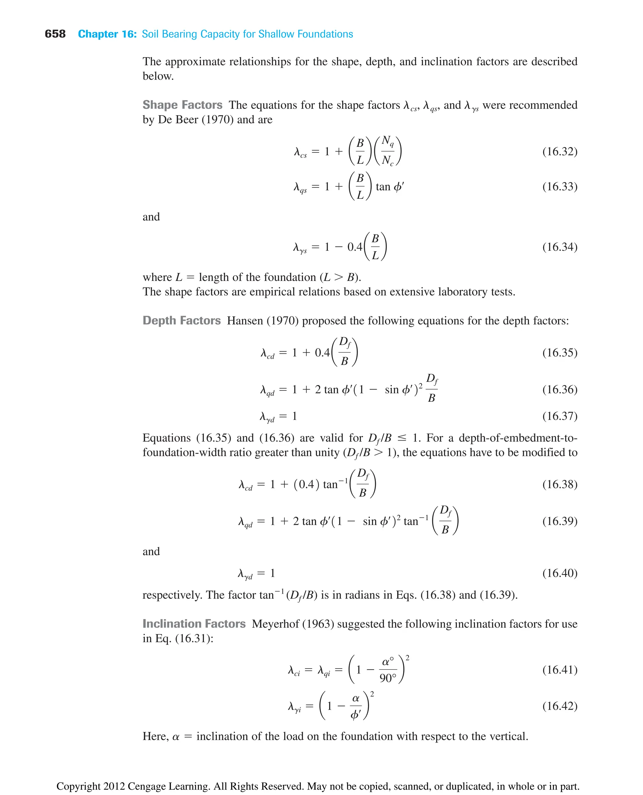
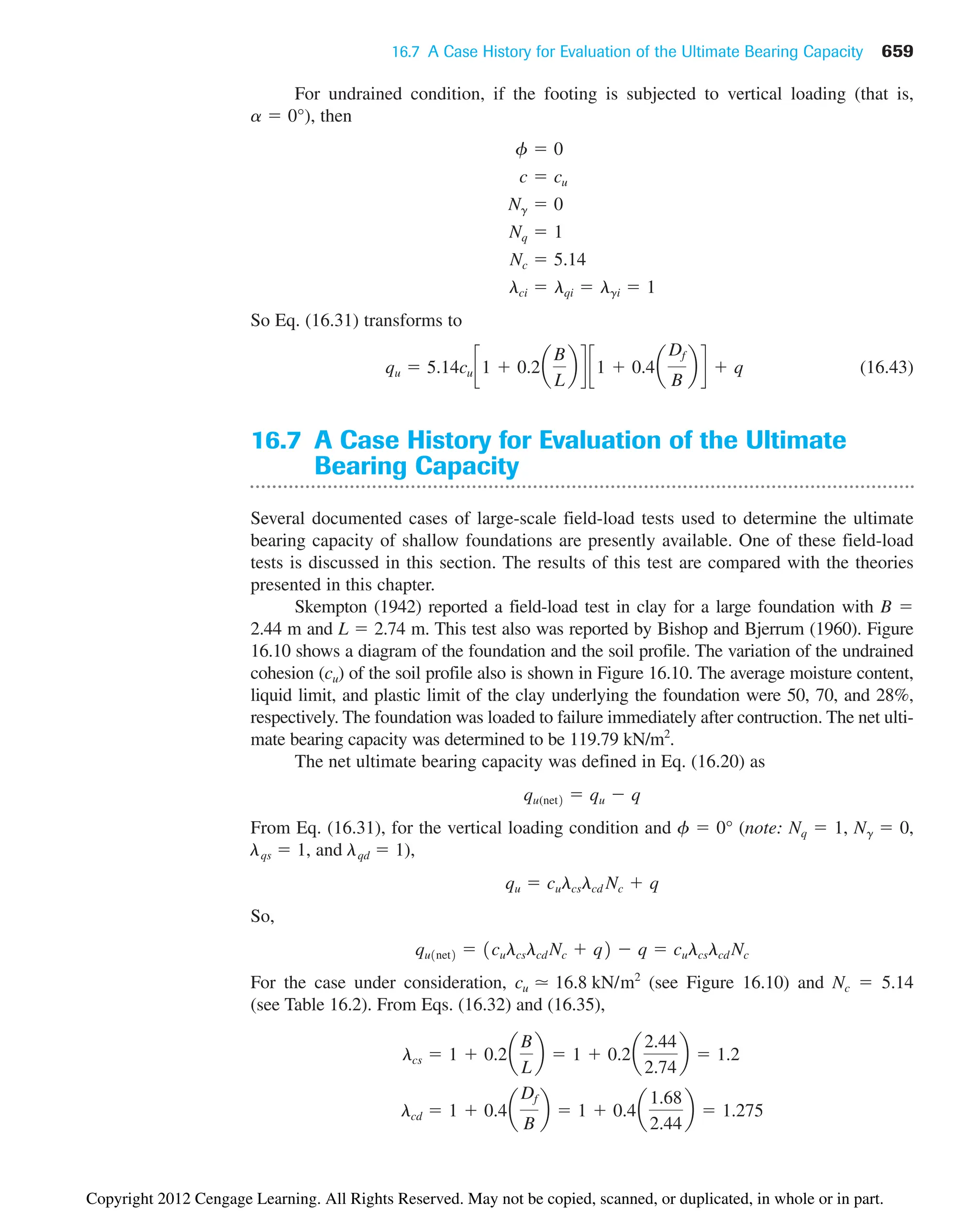
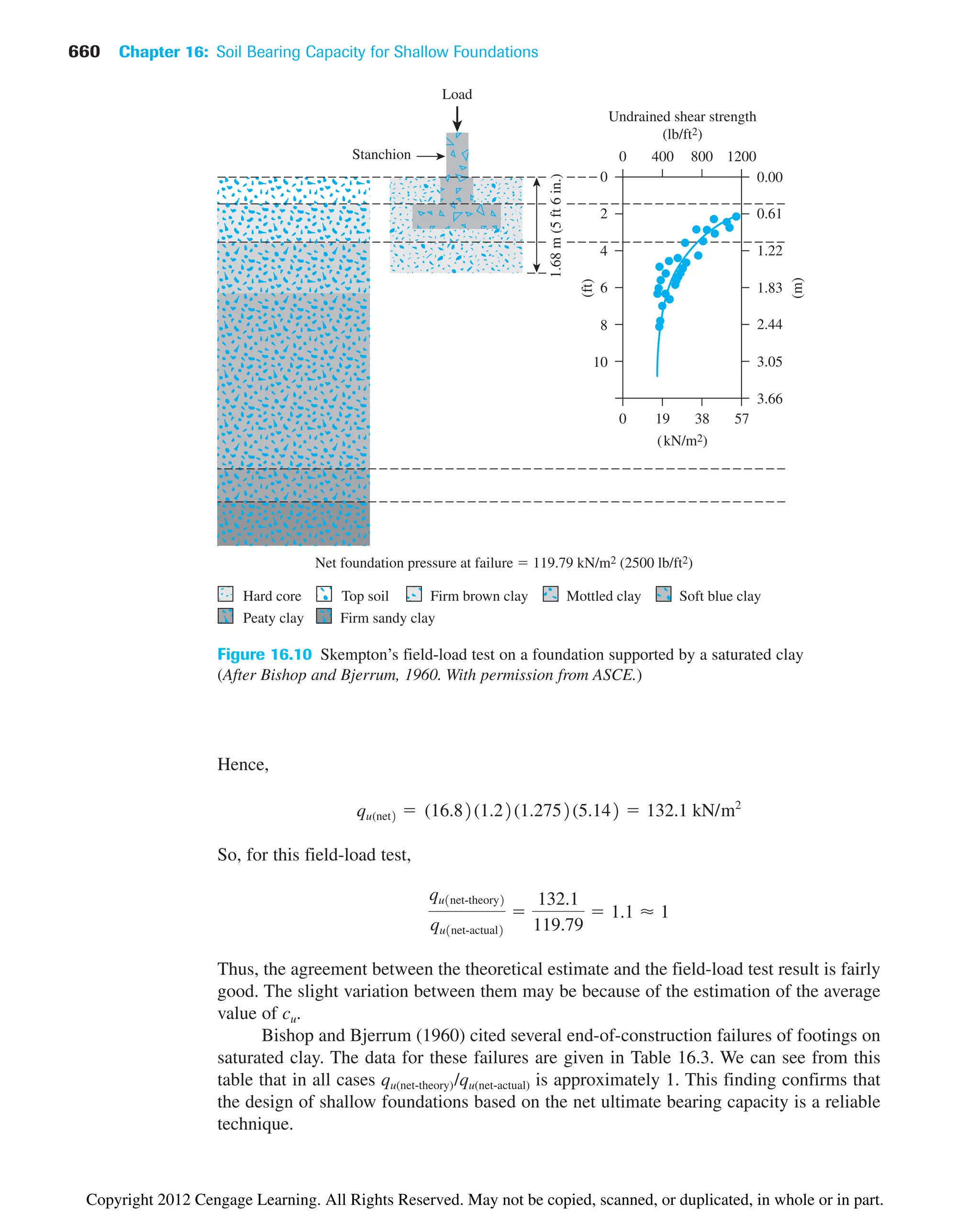
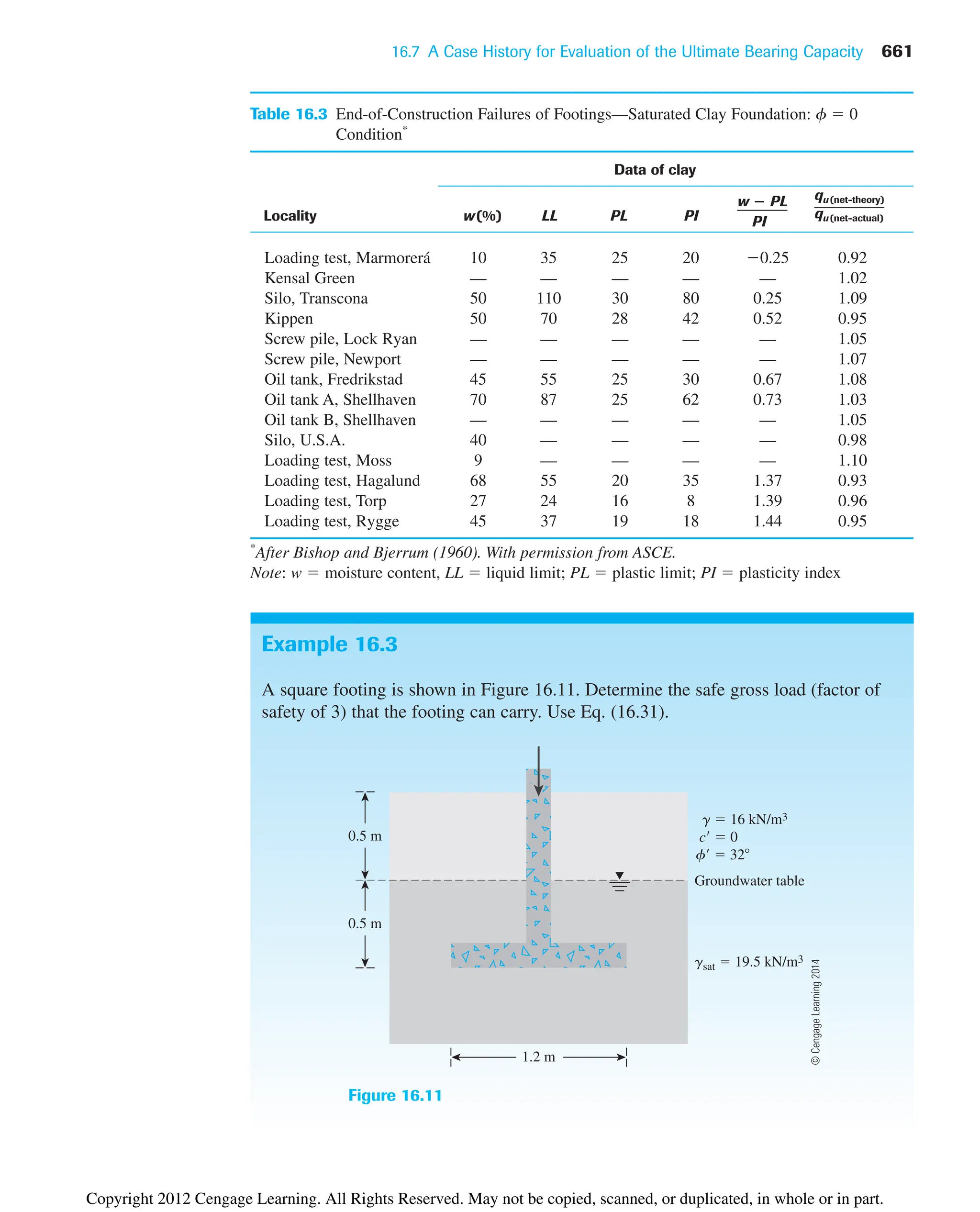
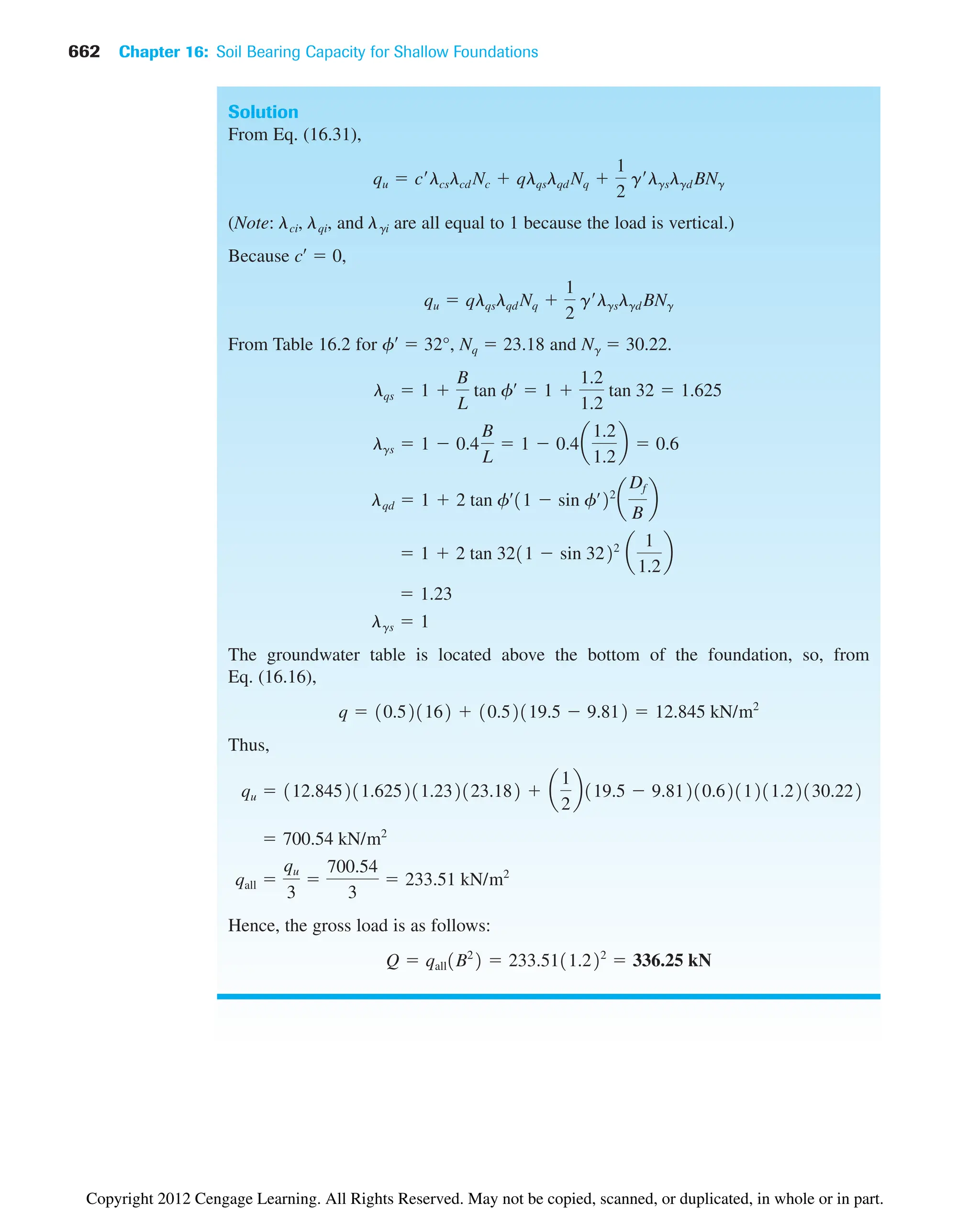
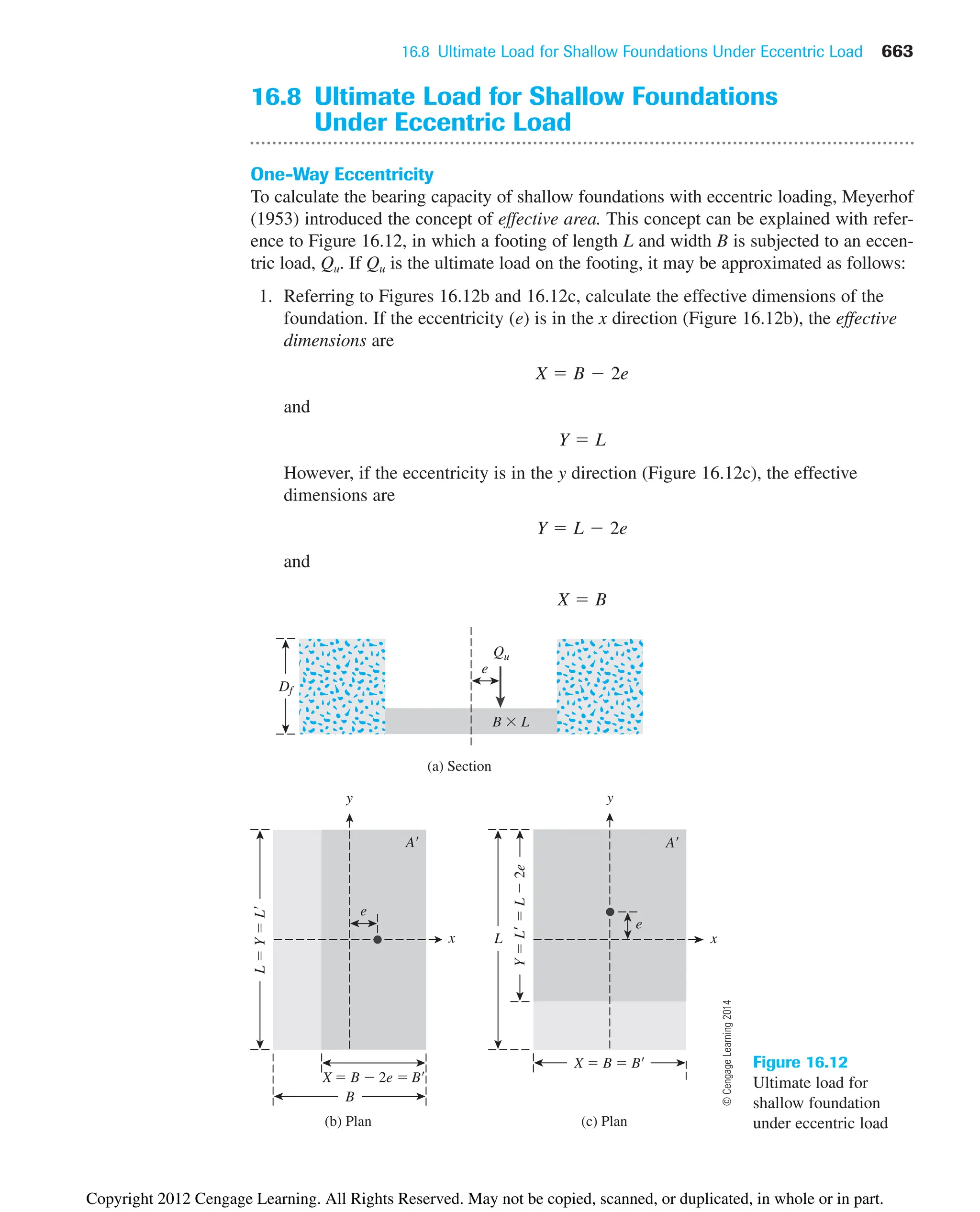
![16.8 Ultimate Load for Shallow Foundations Under Eccentric Load 665
ex
y
(c)
(a)
x
B
B
B
L
ey
y
x
A
B
L L
ex
(b)
y
x
B
L
L
ey
A
ex
A
Figure 16.13
Foundation subjected to
two-way eccentricity
where Qu(eccentric) and Qu(centric) ultimate load per unit length, respectively, for eccentri-
cally and centrically loaded foundations.
Table 16.4 Variations of a and k [Eq. (16.47)]
Df /B a k
0 1.862 0.73
0.25 1.811 0.785
0.5 1.754 0.80
1.0 1.820 0.888
Two-Way Eccentricity
When foundations are subjected to loads with two-way eccentricity, as shown in
Figure 16.13, the effective area is determined such that its centroid coincides with the load.
The procedure for finding the effective dimensions, B¿ and L¿, are beyond the scope of this
text and readers may refer to Das (2011). Once B¿ and L¿ are determined, Eqs. (16.44) and
(16.45) may be used to determine the ultimate load.
©
Cengage
Learning
2014
©
Cengage
Learning
2014
Copyright 2012 Cengage Learning. All Rights Reserved. May not be copied, scanned, or duplicated, in whole or in part.](https://image.slidesharecdn.com/principlesofgeotechnicalengineering-8thedition-231222125509-7e44d9bf/75/Principles-of-Geotechnical-Engineering-8th-Edition-pdf-685-2048.jpg)
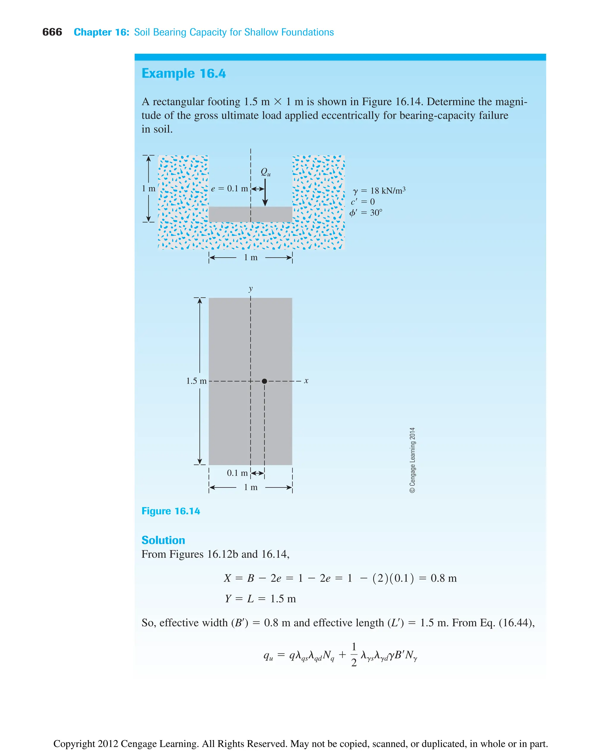
![16.8 Ultimate Load for Shallow Foundations Under Eccentric Load 667
From Table 16.2 for f¿ 30°, Nq 18.4 and N␥ 22.4. Also,
So
Hence, from Eq. (16.45),
Qu qu1Bœ
Lœ
2 1716.53210.8211.52 859.8 kN
a
1
2
b10.787211.02118210.82122.42 716.53 kN/m2
qu 11 18211.308211.3612118.42
lgd 1
1.361
1 2 tan 30 11 sin 3022
a
1
0.8
b
lqd 1 2 tan fœ
11 sin fœ
22
a
Df
B
b
lgs 1 0.4a
0.8
1.5
b 0.787
lqs 1
Bœ
Lœ tan fœ
1 a
0.8
1.5
b tan 30 1.308
Example 16.5
Consider an eccentrically loaded continuous foundation supported by a granular soil.
Given: B 1.5 m, Df 0.75 m, load eccentricity e/B 0.1, ␥ 17.5 kN/m3
, f¿ 30°,
and c¿ 0. Use the reduction factor method [Eq. (16.48)] and determine the gross
ultimate load per unit length that the foundation can carry.
Solution
From Eq. (16.48),
Also, Df /B 0.75/1.5 0.5. From Table 16.4, a 1.754 and k 0.8. Thus,
(Note: The shape factors are all equal to one, since it is a continuous foundation.)
q gDf 117.5210.752 13.125 kN/m2
Qu1centric2 aqN
qlqd
1
2
lgd BNg bB
Qu1eccentric2 Qu1centric2 c1 aa
e
B
b
k
d
Copyright 2012 Cengage Learning. All Rights Reserved. May not be copied, scanned, or duplicated, in whole or in part.](https://image.slidesharecdn.com/principlesofgeotechnicalengineering-8thedition-231222125509-7e44d9bf/75/Principles-of-Geotechnical-Engineering-8th-Edition-pdf-687-2048.jpg)
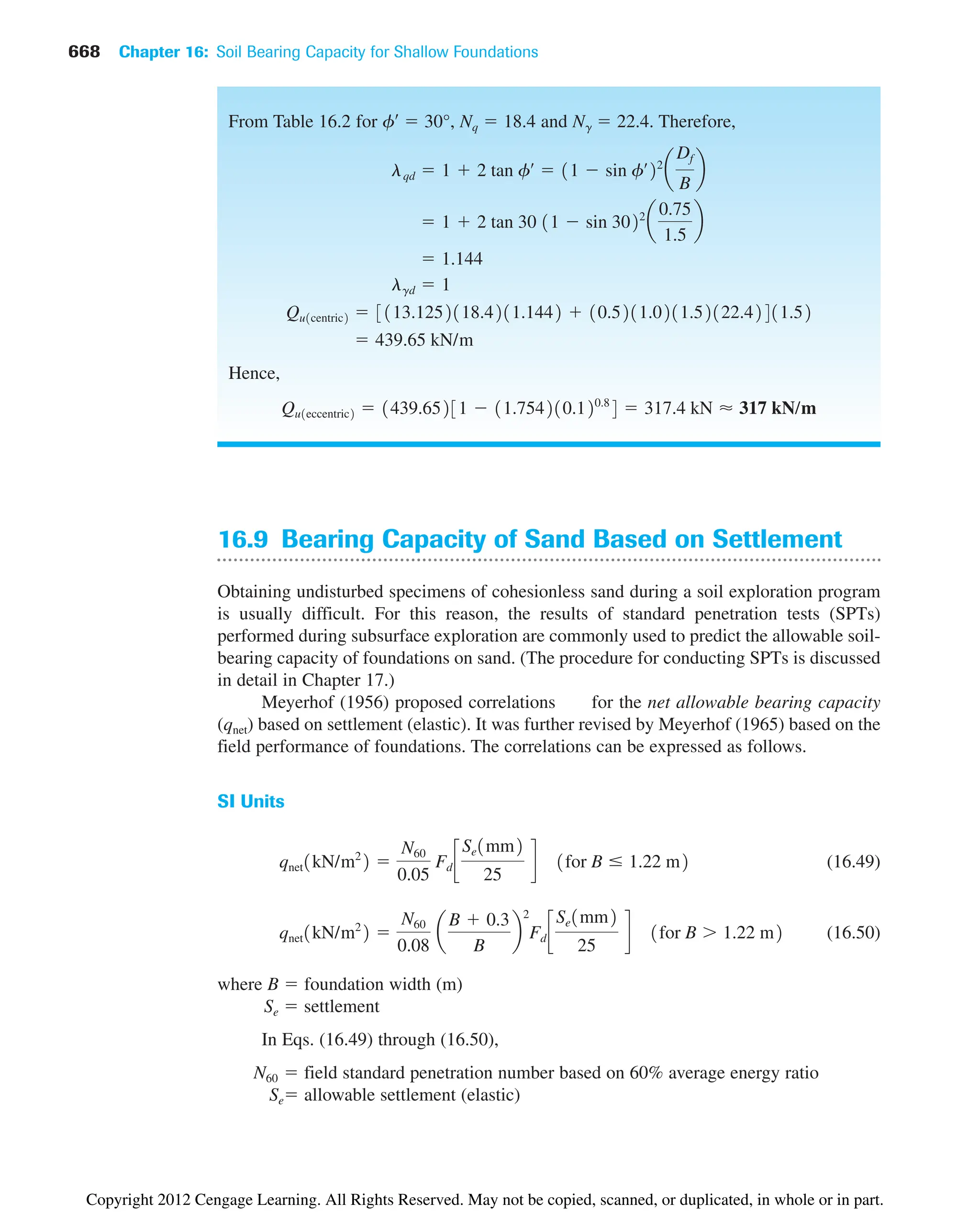
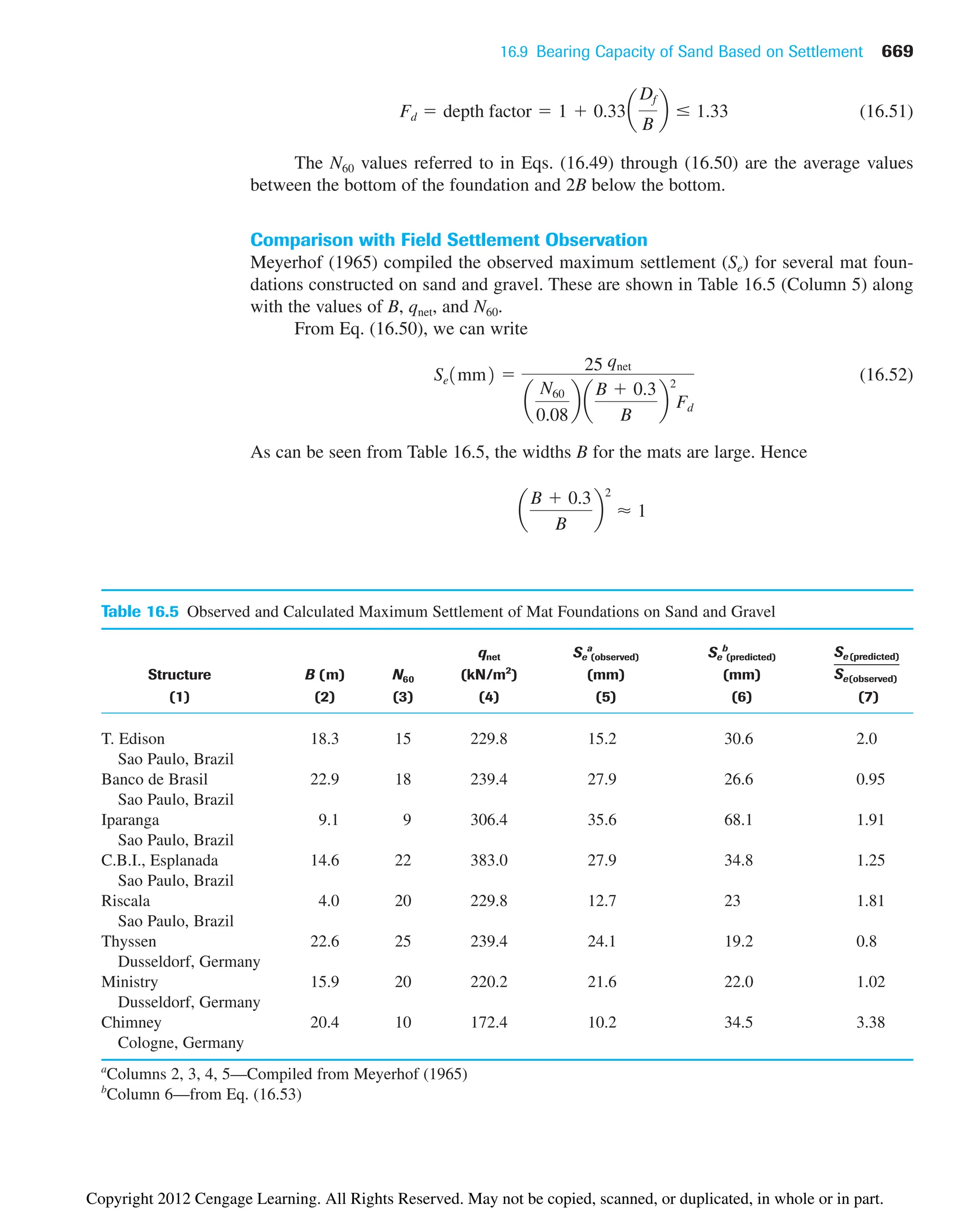
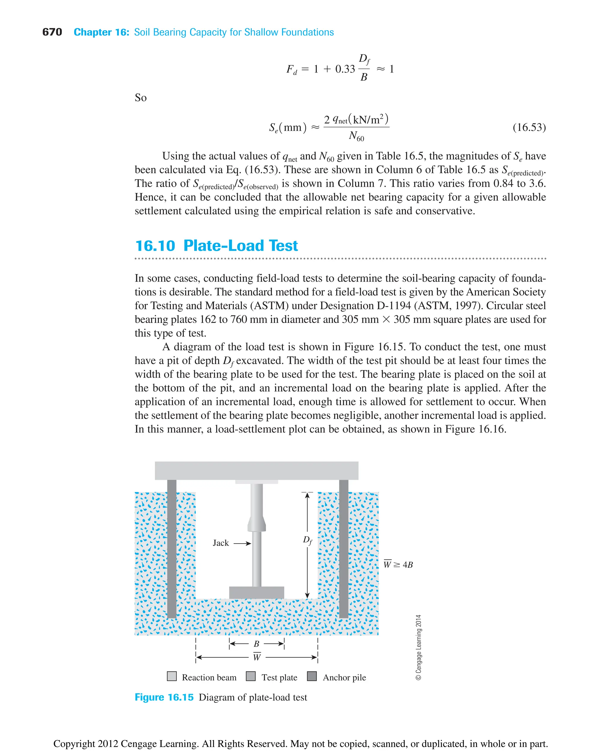
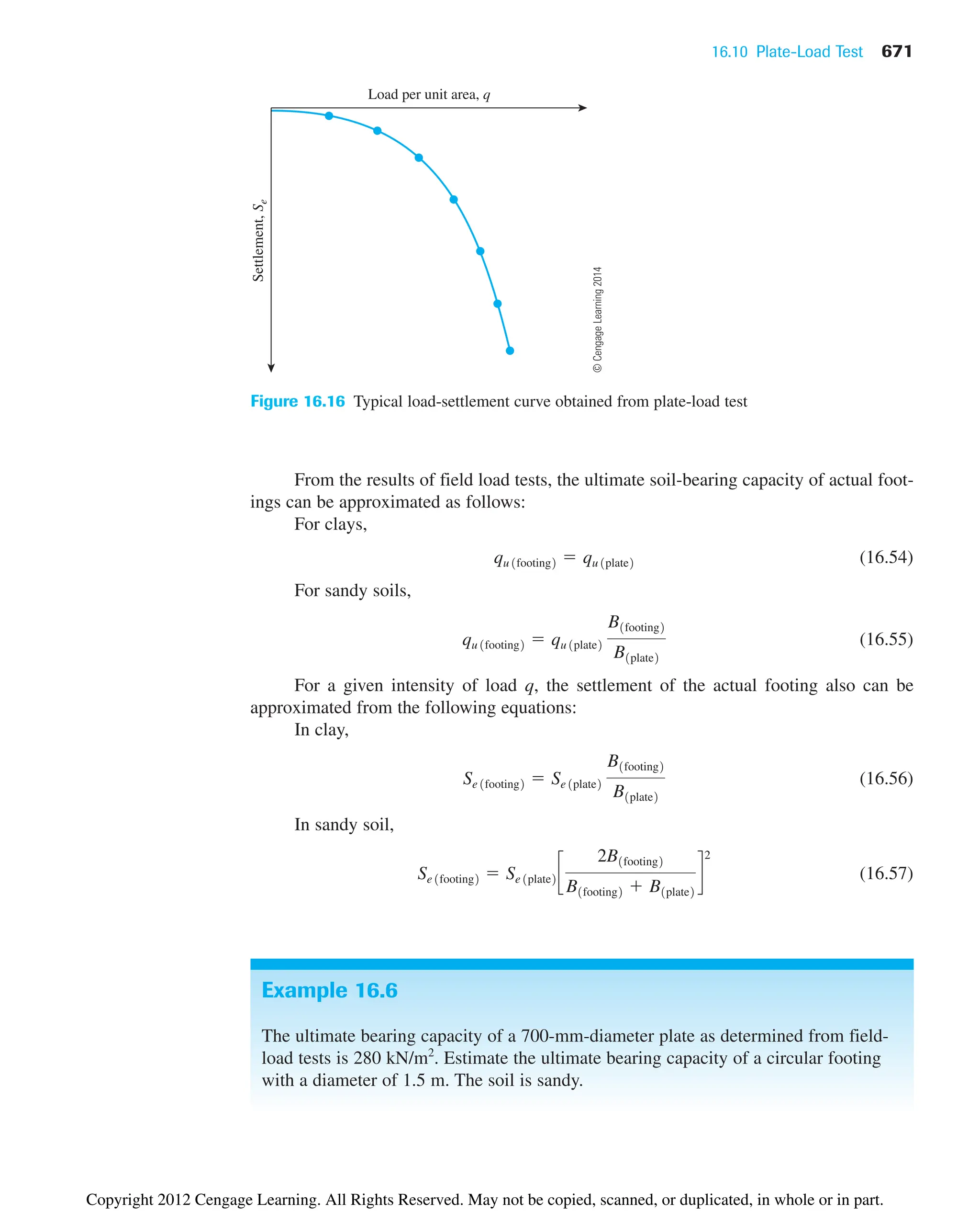
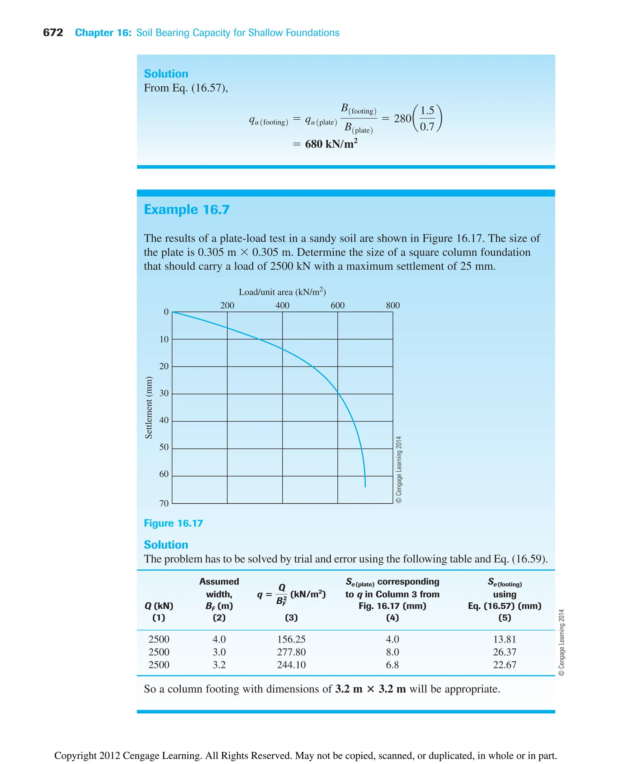
![Problems 673
16.11 Summary and General Comments
In this chapter, theories for estimating the ultimate and allowable bearing capacities of
shallow foundations were presented. Procedures for field-load tests and estimation of the
allowable bearing capacity of granular soil based on limited settlement criteria were dis-
cussed briefly.
Following is an itemized list of the important materials covered in this chapter.
• Terzaghi’s ultimate bearing-capacity equations [Eqs. (16.11), (16.12), and (16.13)]
• General ultimate bearing-capacity equation [Eq. (16.31)]
• Ultimate bearing capacity of foundations subjected to vertical eccentric load
[Eq. (16.44)]
• Bearing capacity of shallow foundations based on settlement (Section 16.9)
Several building codes now used in the United States and elsewhere provide pre-
sumptive bearing capacities for various types of soil. It is extremely important to realize
that they are approximate values only. The bearing capacity of foundations depends on
several factors:
1. Subsoil stratification
2. Shear strength parameters of the subsoil
3. Location of the groundwater table
4. Environmental factors
5. Building size and weight
6. Depth of excavation
7. Type of structure
Hence, it is important that the allowable bearing capacity at a given site be determined based
on the findings of soil exploration at that site, past experience of foundation construction,
and fundamentals of the geotechnical engineering theories for bearing capacity.
The allowable bearing-capacity relationships based on settlement considerations such
as those given in Section 16.10 do not take into account the settlement caused by consoli-
dation of the clay layers. Excessive settlement usually causes the building to crack, which
ultimately may lead to structural failure. Uniform settlement of a structure does not produce
cracking; on the other hand, differential settlement may produce cracks and damage to a
building.
Problems
16.1 A continuous footing is shown in Figure 16.18. Using Terzaghi’s bearing-capacity
factors, determine the gross allowable load per unit area (qall) that the footing can
carry. Assume general shear failure. Given: ␥ 17.5 kN/m3
, c 21 kN/m2
,
f 32°, Df 1 m, B 1.5 m, and factor of safety 3.
16.2 Repeat Problem 16.1 with the following: ␥ 18.5 kN/m3
, c 71.8 kN/m2
,
f 24°, Df 1.21 m, B 1.83 m, and factor of safety 4.
16.3 Repeat Problem 16.1 with the following: ␥ 19.5 kN/m3
, cu 37 kN/m2
,
f 0, Df 0.75 m, B 2.5 m, and factor of safety 6.
16.4 Repeat Problem 16.1 using the modified general ultimate bearing capacity,
Eq. (16.31).
Copyright 2012 Cengage Learning. All Rights Reserved. May not be copied, scanned, or duplicated, in whole or in part.](https://image.slidesharecdn.com/principlesofgeotechnicalengineering-8thedition-231222125509-7e44d9bf/75/Principles-of-Geotechnical-Engineering-8th-Edition-pdf-693-2048.jpg)
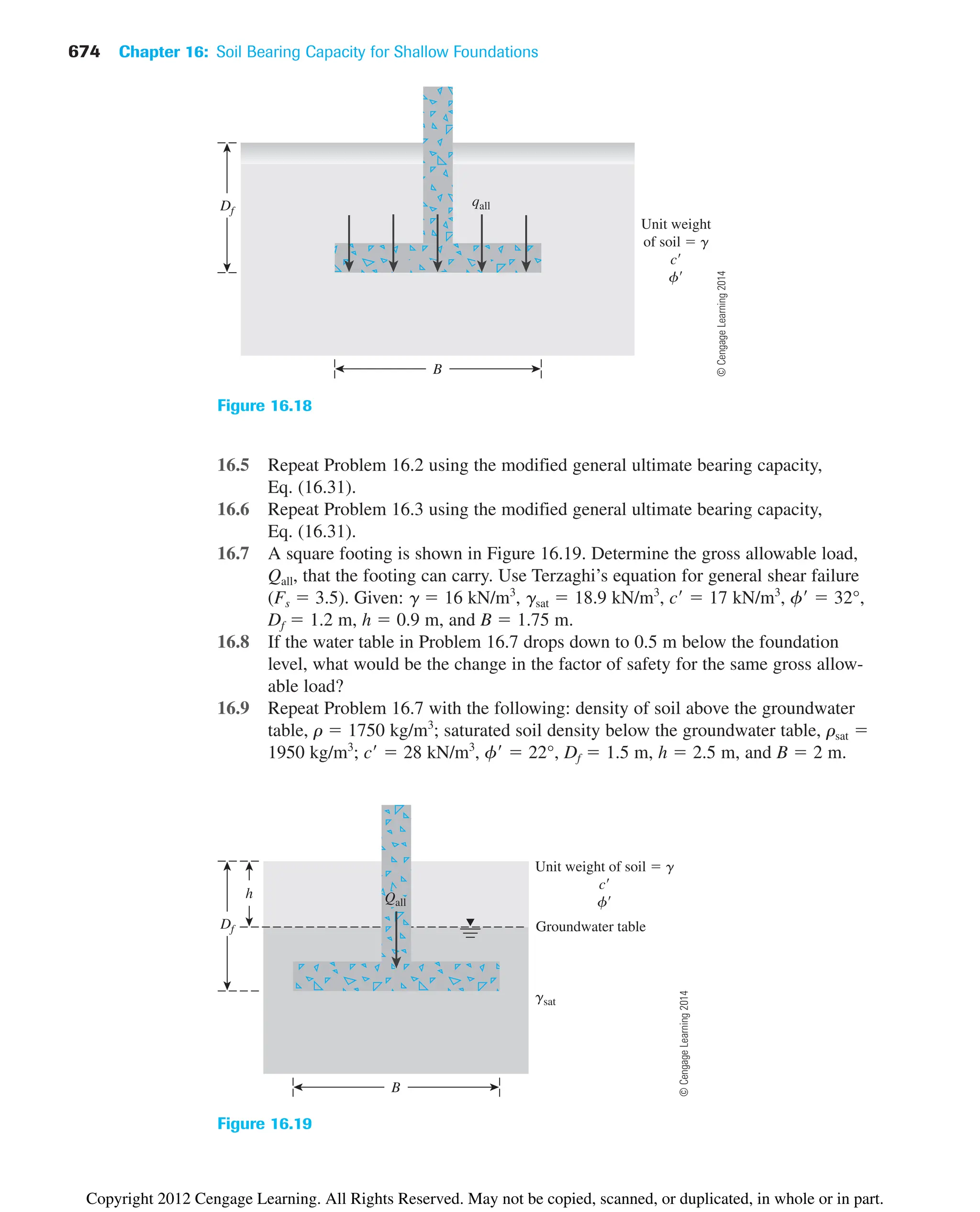
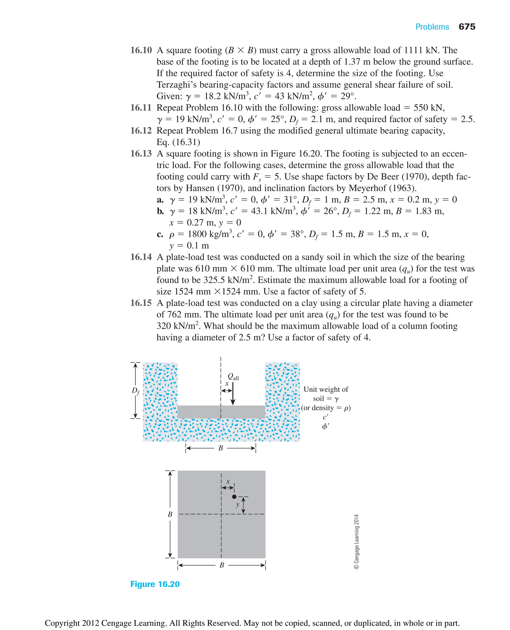
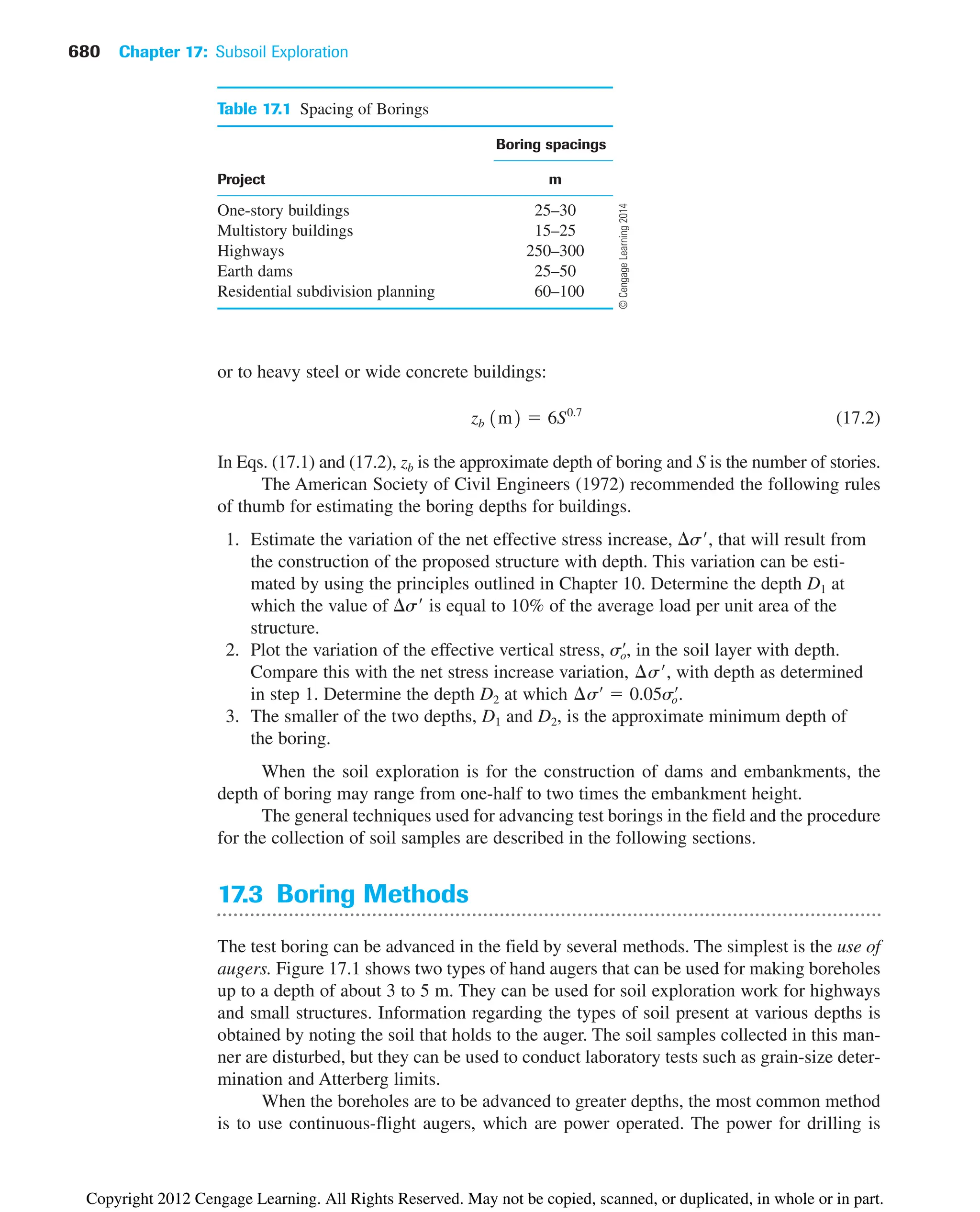
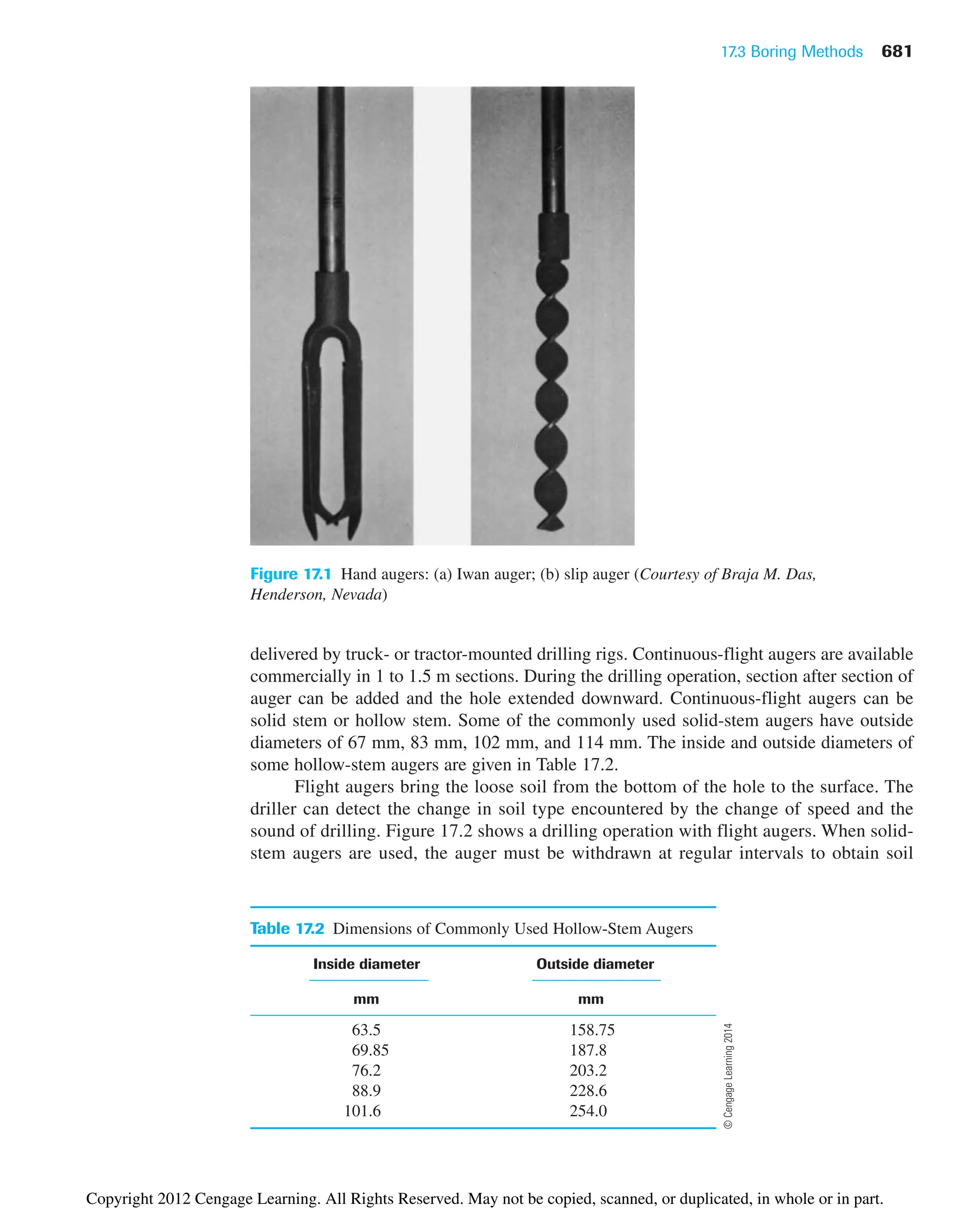
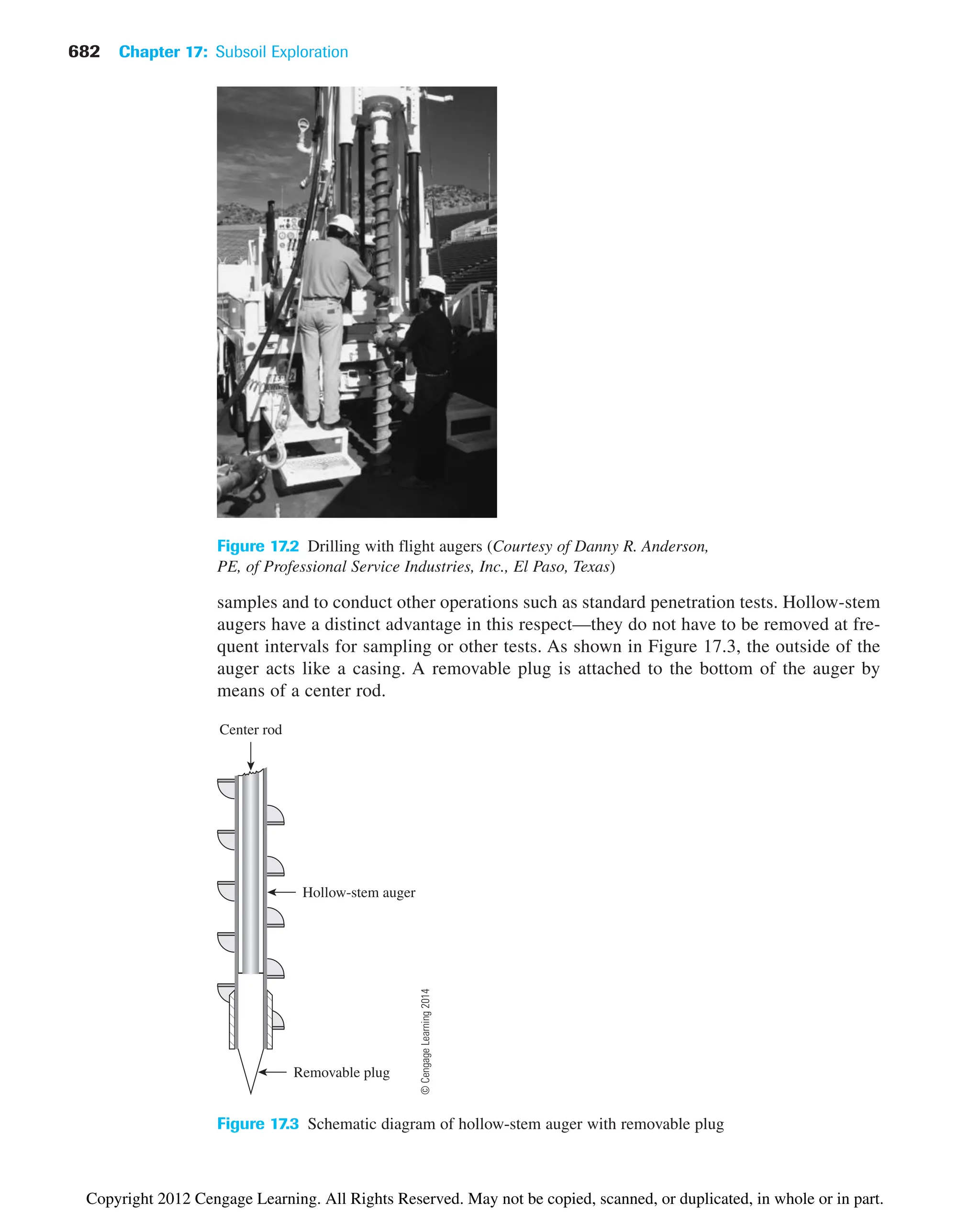
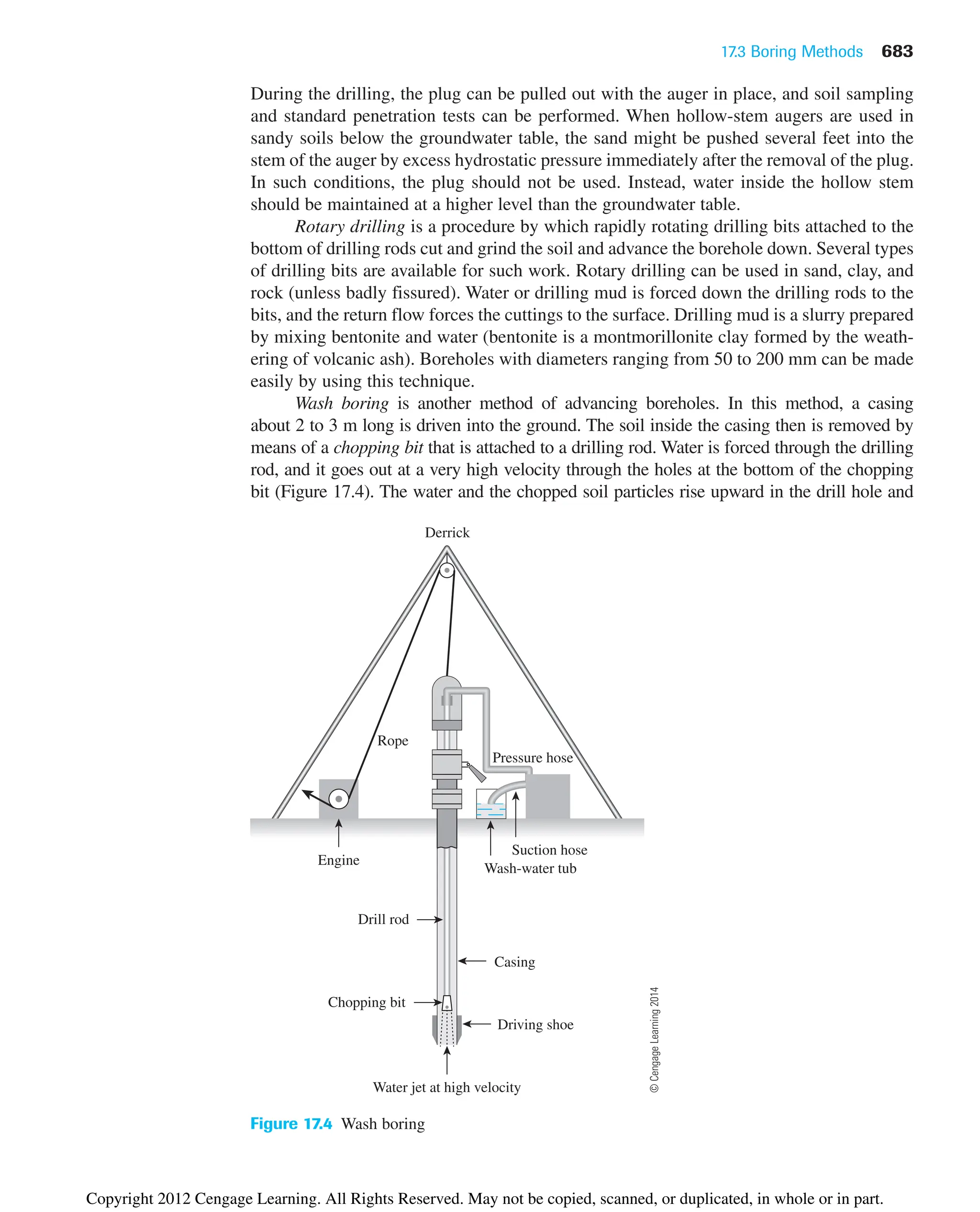
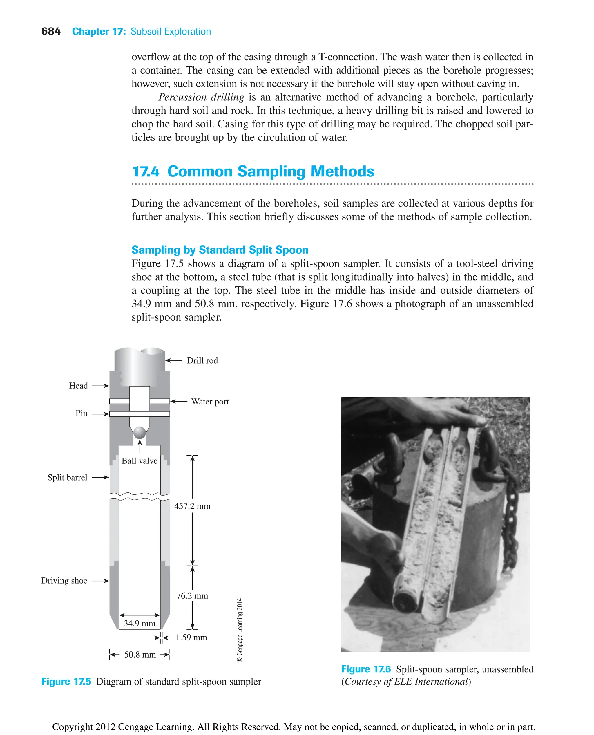
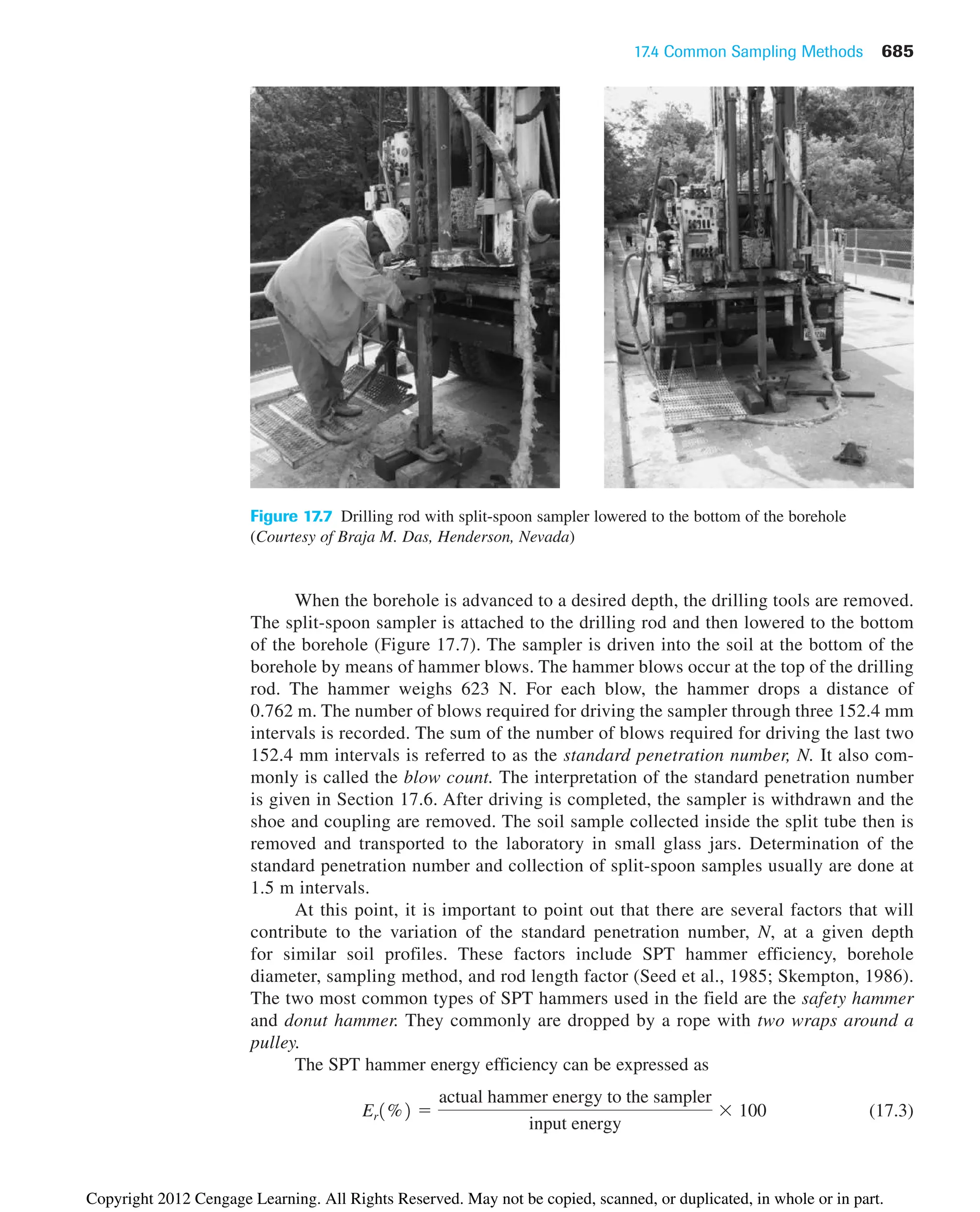
![686 Chapter 17: Subsoil Exploration
(17.4)
where W ⫽ weight of the hammer ⬇ 0.623 kN
h ⫽ height of drop ⬇ 0.76 mm
So,
In the field, the magnitude of Er can vary from 30 to 90%. The standard practice now in
the U.S. is to express the N-value to an average energy ratio of 60% (⬇ N60). Thus, cor-
recting for field procedures and on the basis of field observations, it appears reasonable to
standardize the field penetration number as a function of the input driving energy and its
dissipation around the sampler into the surrounding soil, or
(17.5)
where N60 ⫽ standard penetration number corrected for field conditions
N ⫽ measured penetration number
hH ⫽ hammer efficiency (%)
hB ⫽ correction for borehole diameter
hS ⫽ sampler correction
hR ⫽ correction for rod length
Based on the recommendations of Seed et al. (1985) and Skempton (1986), the vari-
ations of hH, hB, hS, and hR are summarized in Table 17.3.
N60 ⫽
NhHhBhShR
60
Wh ⫽ 10.623210.762 ⫽ 0.474 kN-m
Theoretical input energy ⫽ Wh
Table 17.3 Variations of hH, hB, hS, and hR [Eq. (17.5)]
1. Variation of HH
Country Hammer type Hammer release HH (%)
Japan Donut Free fall 78
Donut Rope and pulley 67
United States Safety Rope and pulley 60
Donut Rope and pulley 45
Argentina Donut Rope and pulley 45
China Donut Free fall 60
Donut Rope and pulley 50
2. Variation of HB
Diameter
mm HB
60–120 1
150 1.05
200 1.15
(continued)
©
Cengage
Learning
2014
Copyright 2012 Cengage Learning. All Rights Reserved. May not be copied, scanned, or duplicated, in whole or in part.](https://image.slidesharecdn.com/principlesofgeotechnicalengineering-8thedition-231222125509-7e44d9bf/75/Principles-of-Geotechnical-Engineering-8th-Edition-pdf-706-2048.jpg)
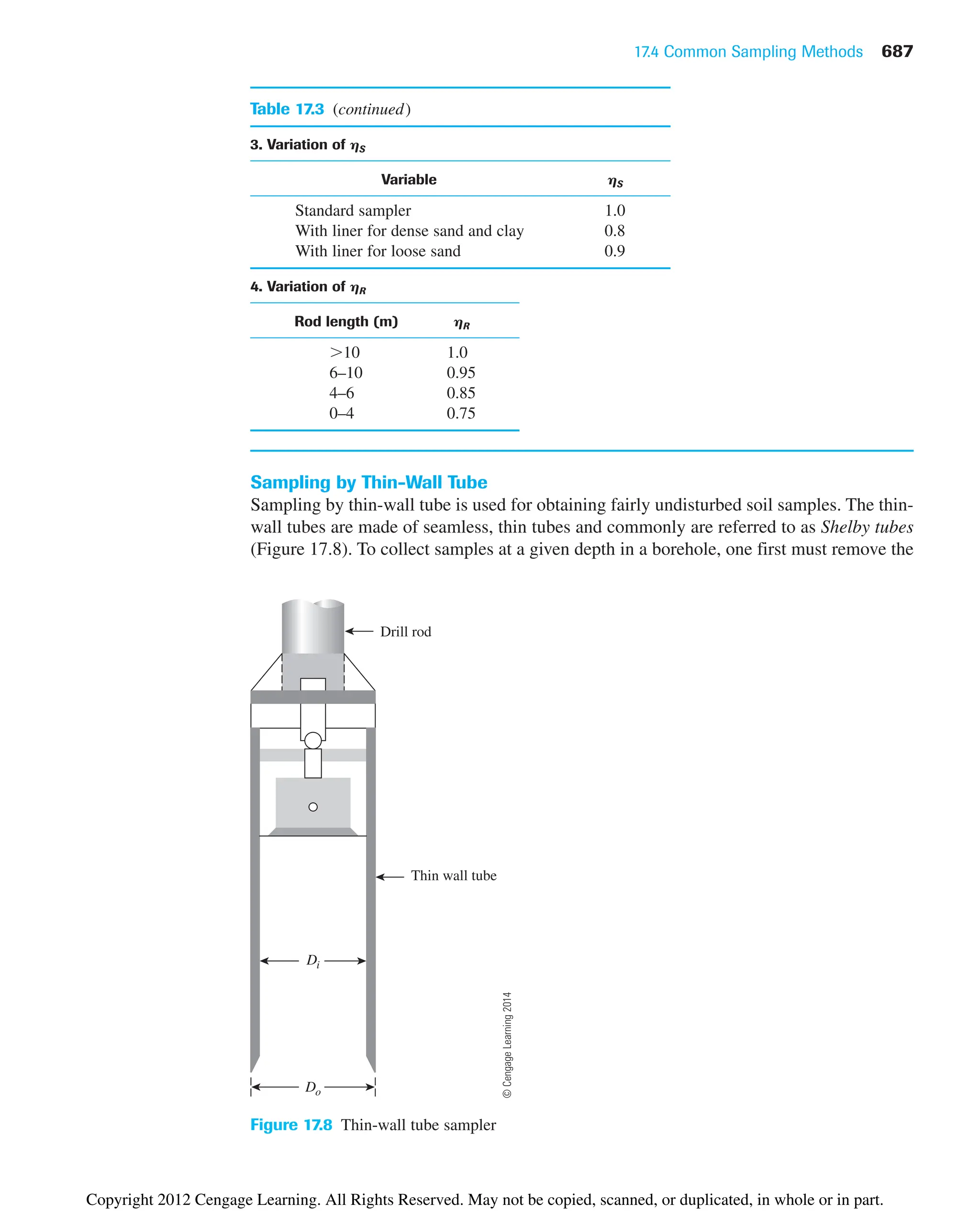
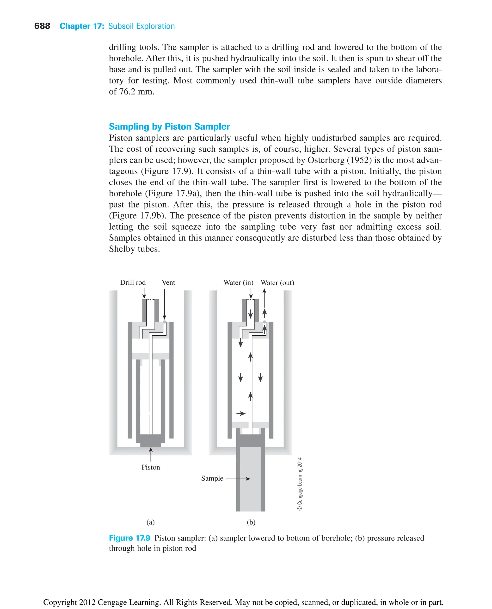
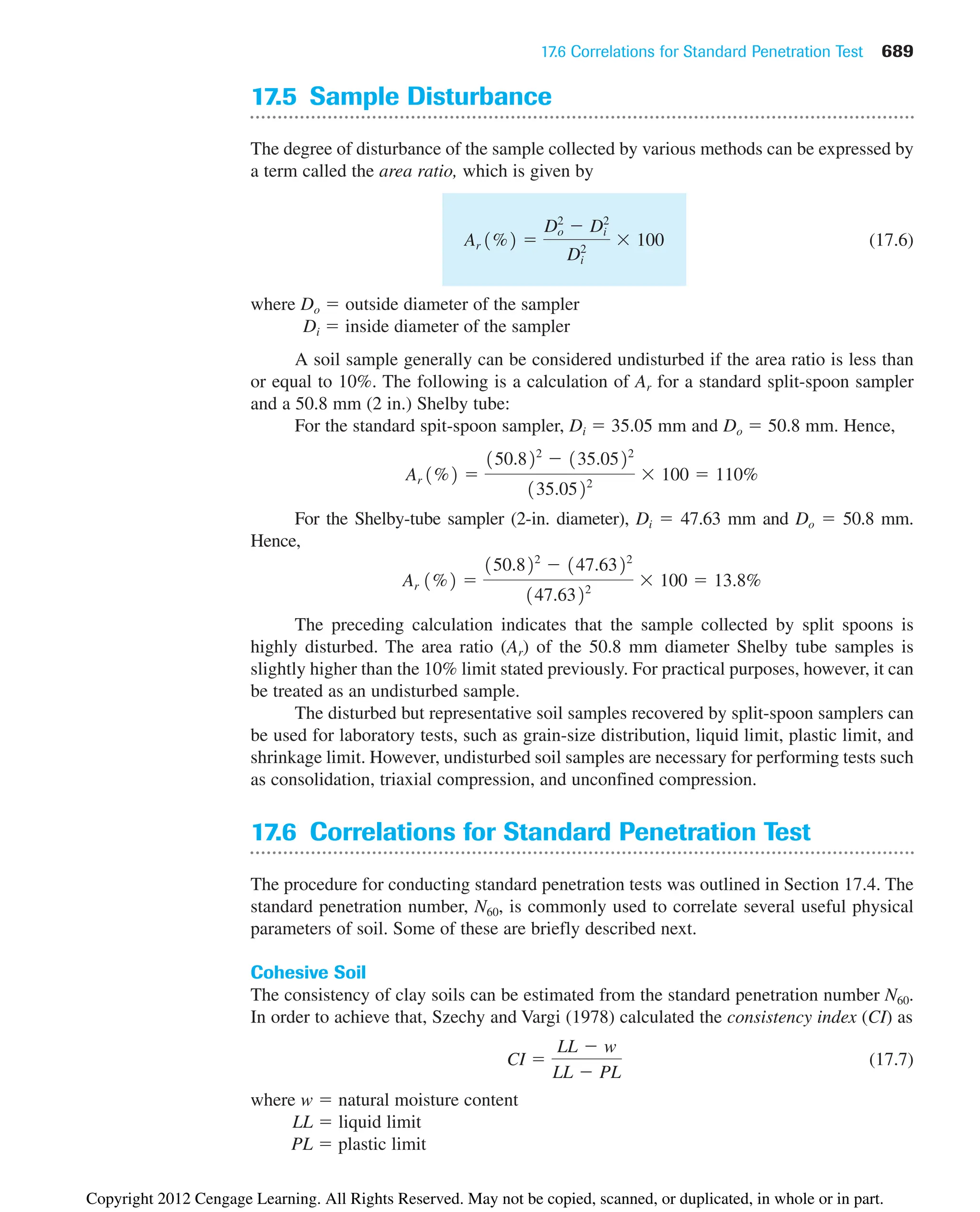
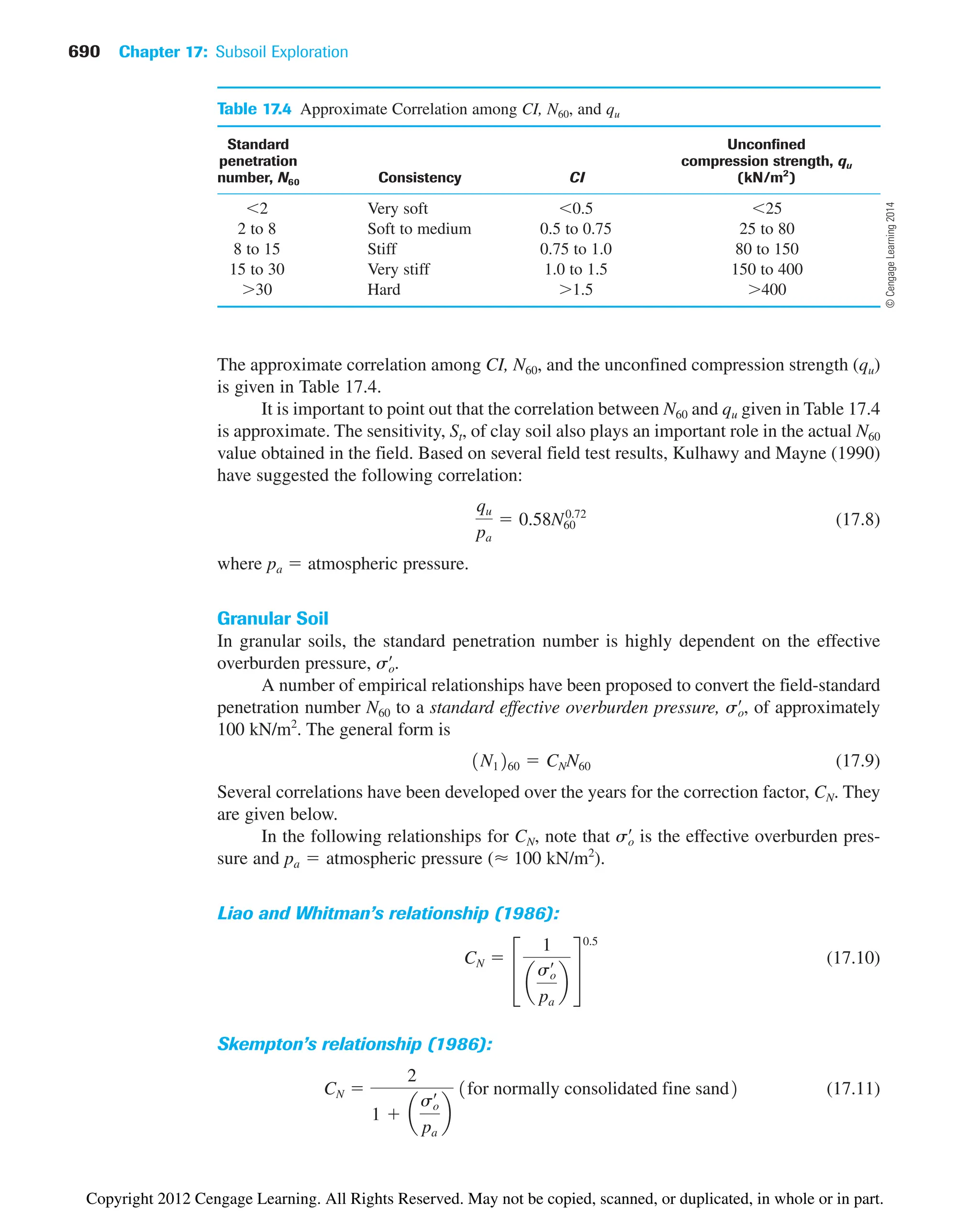
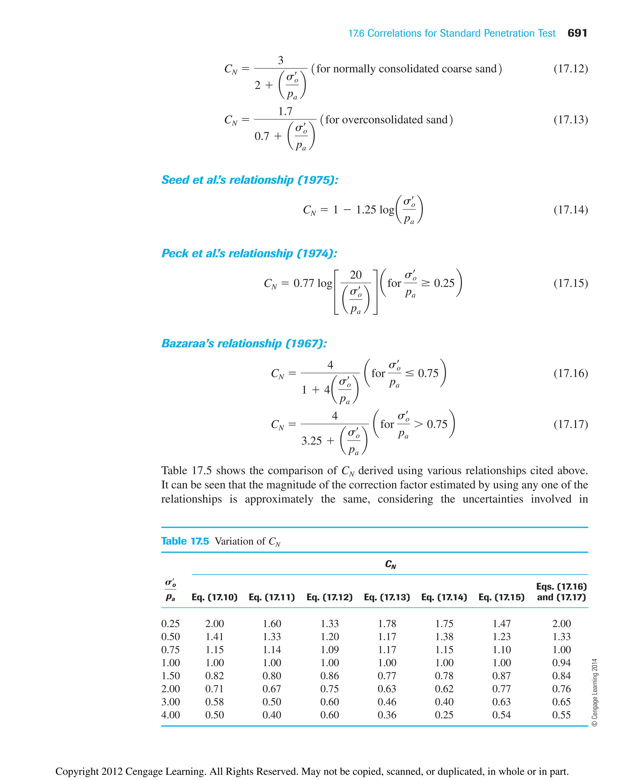
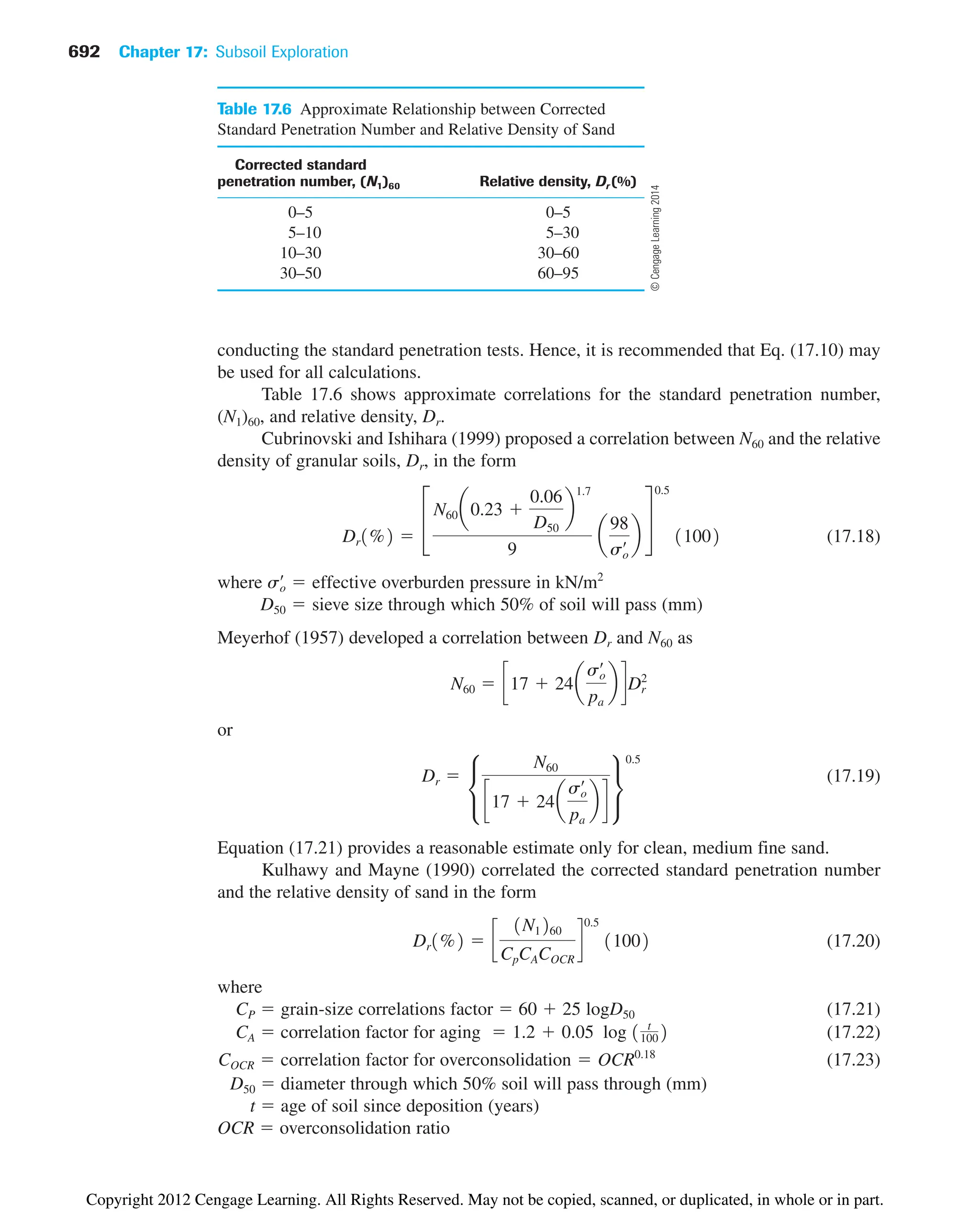
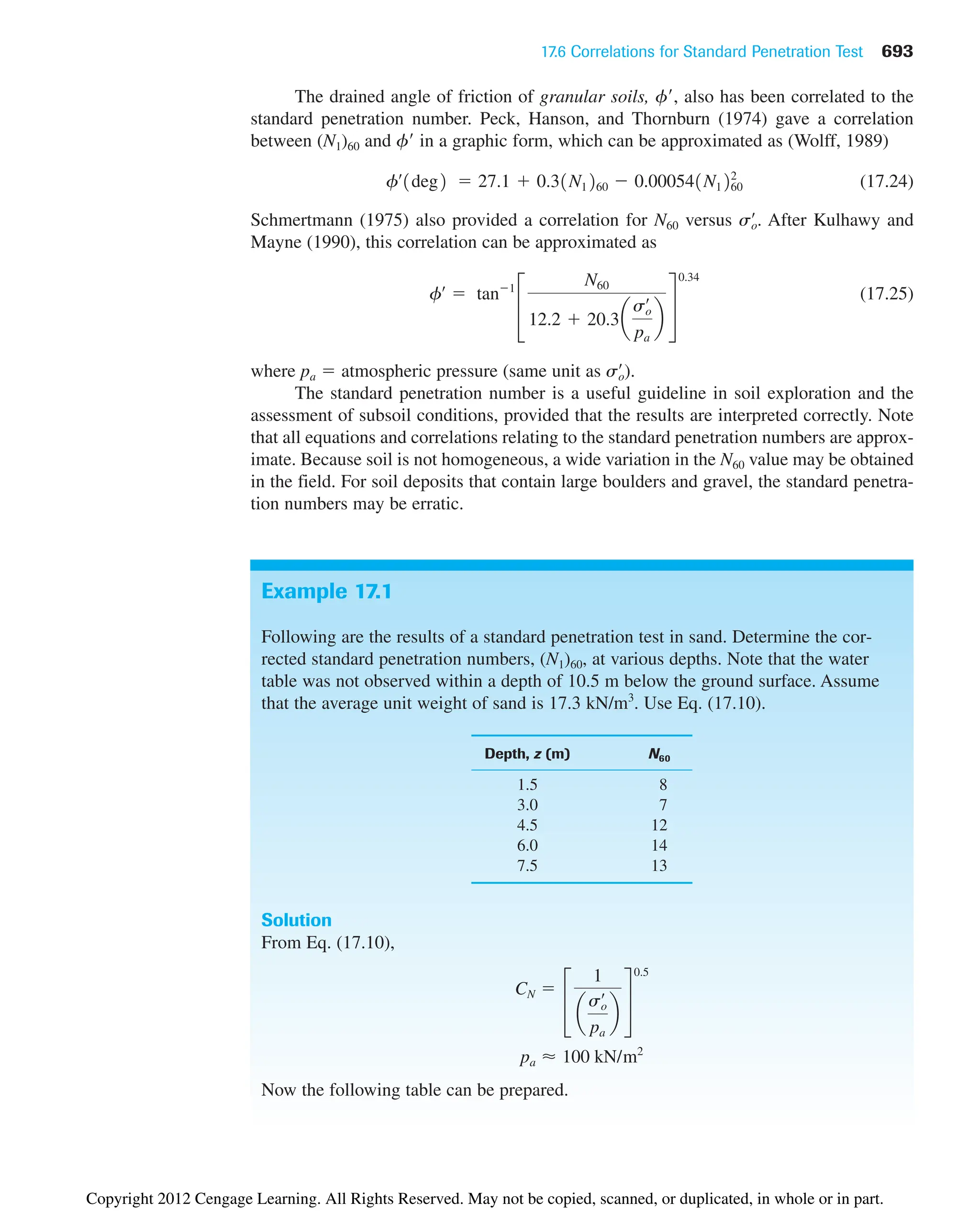
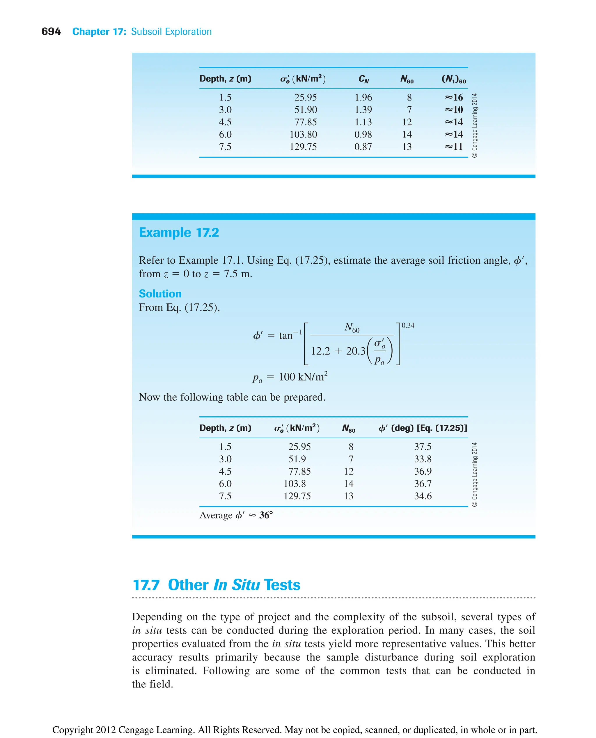
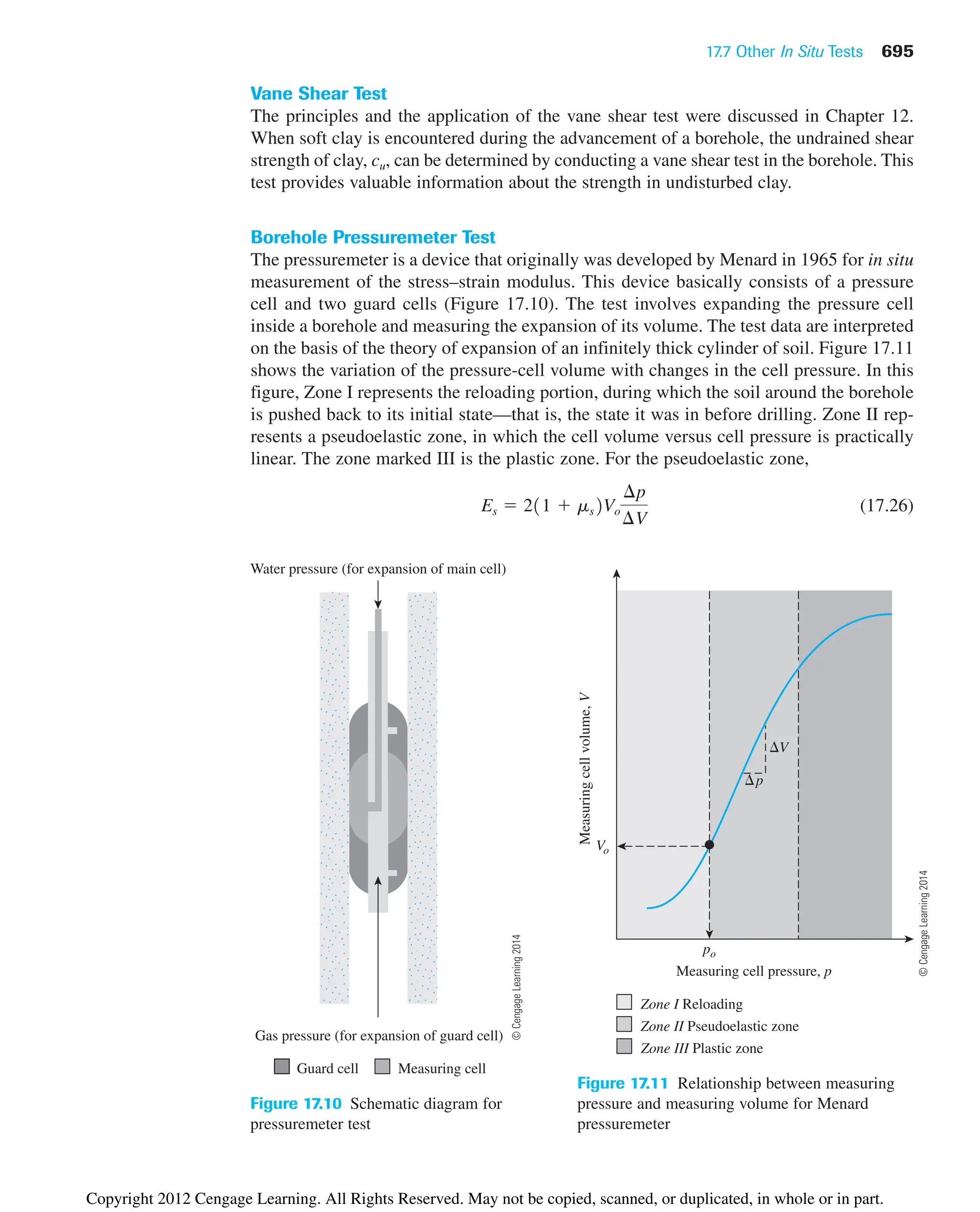
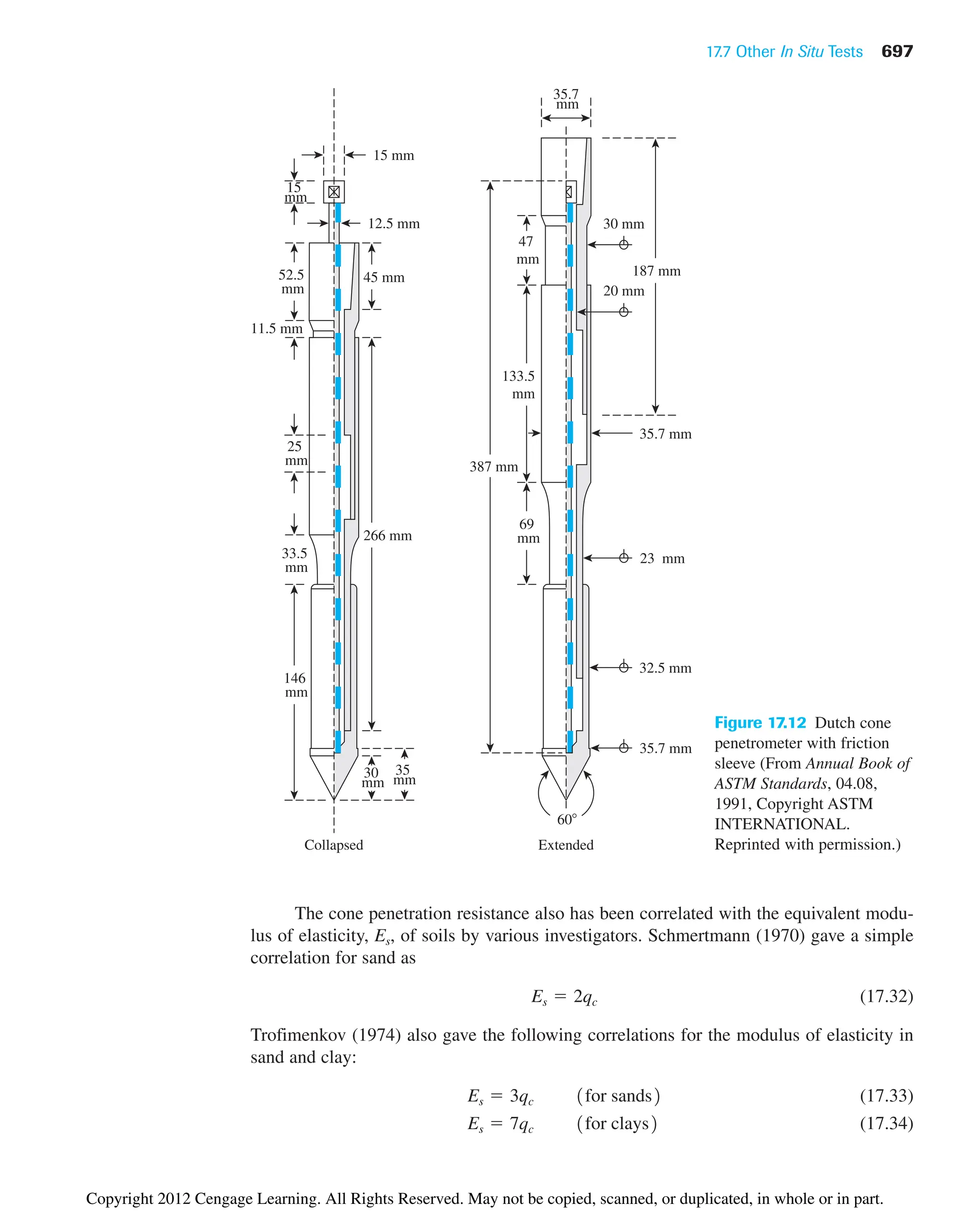
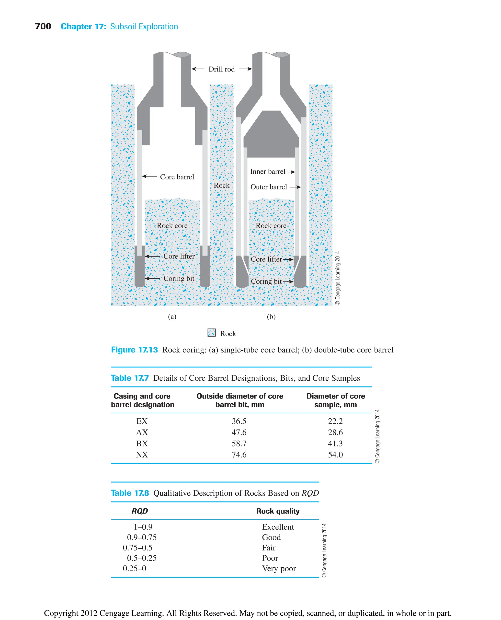
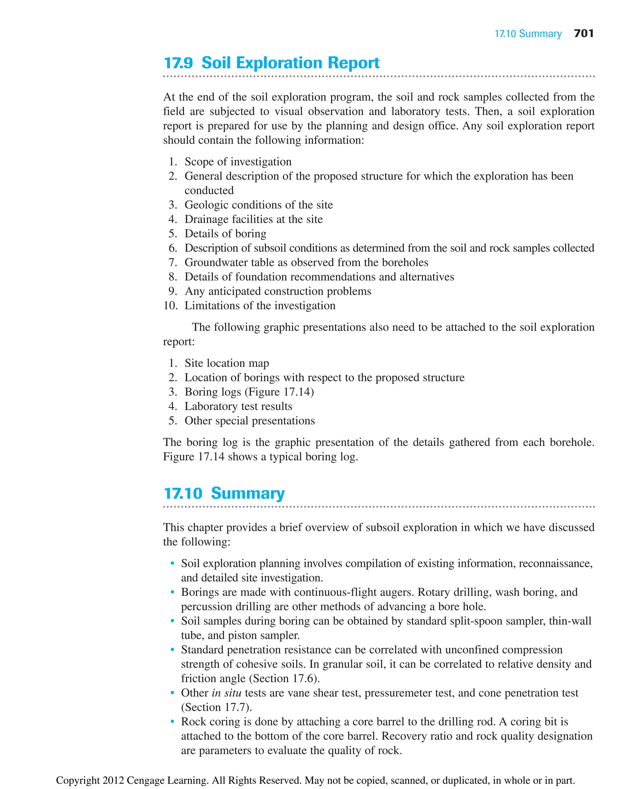
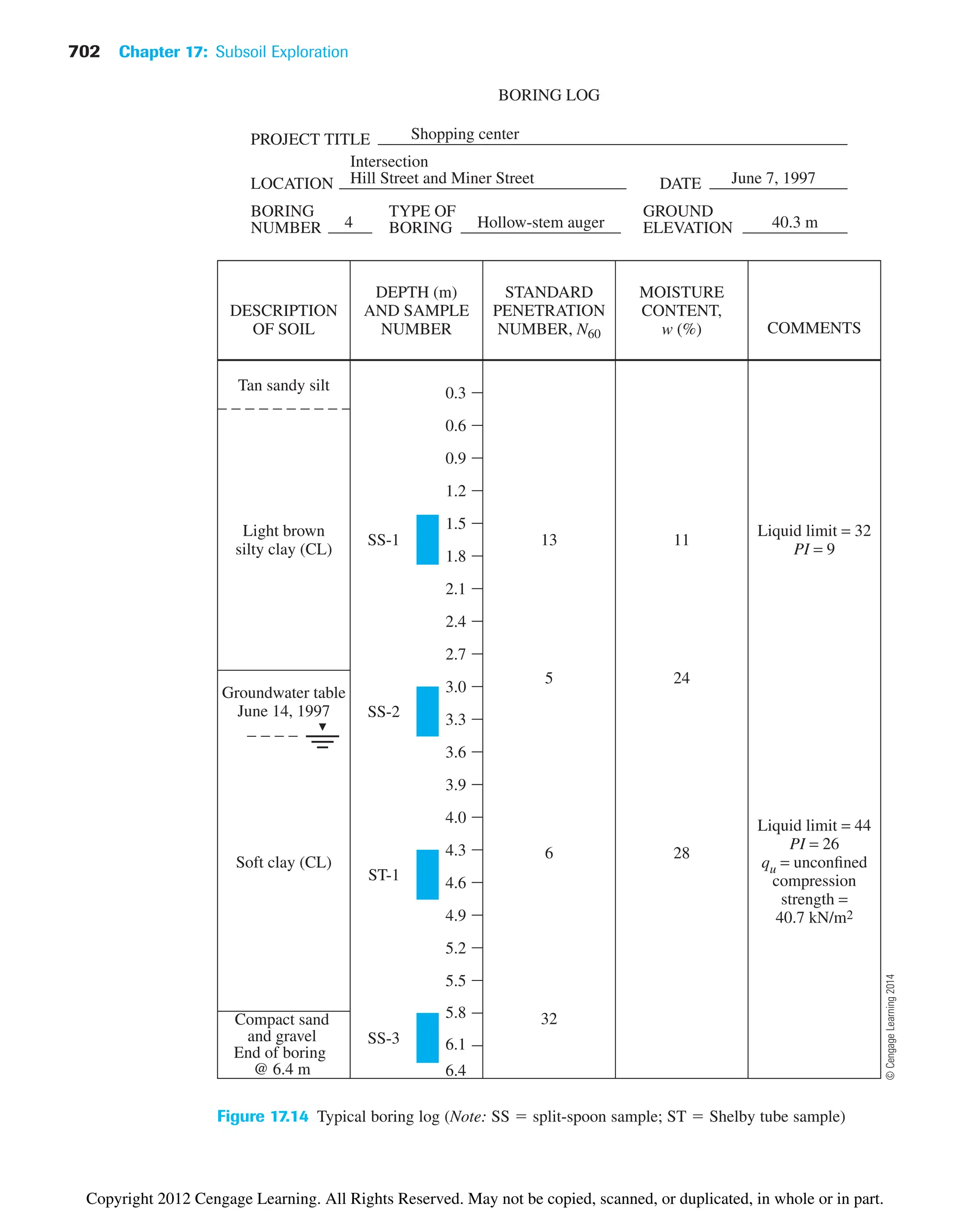
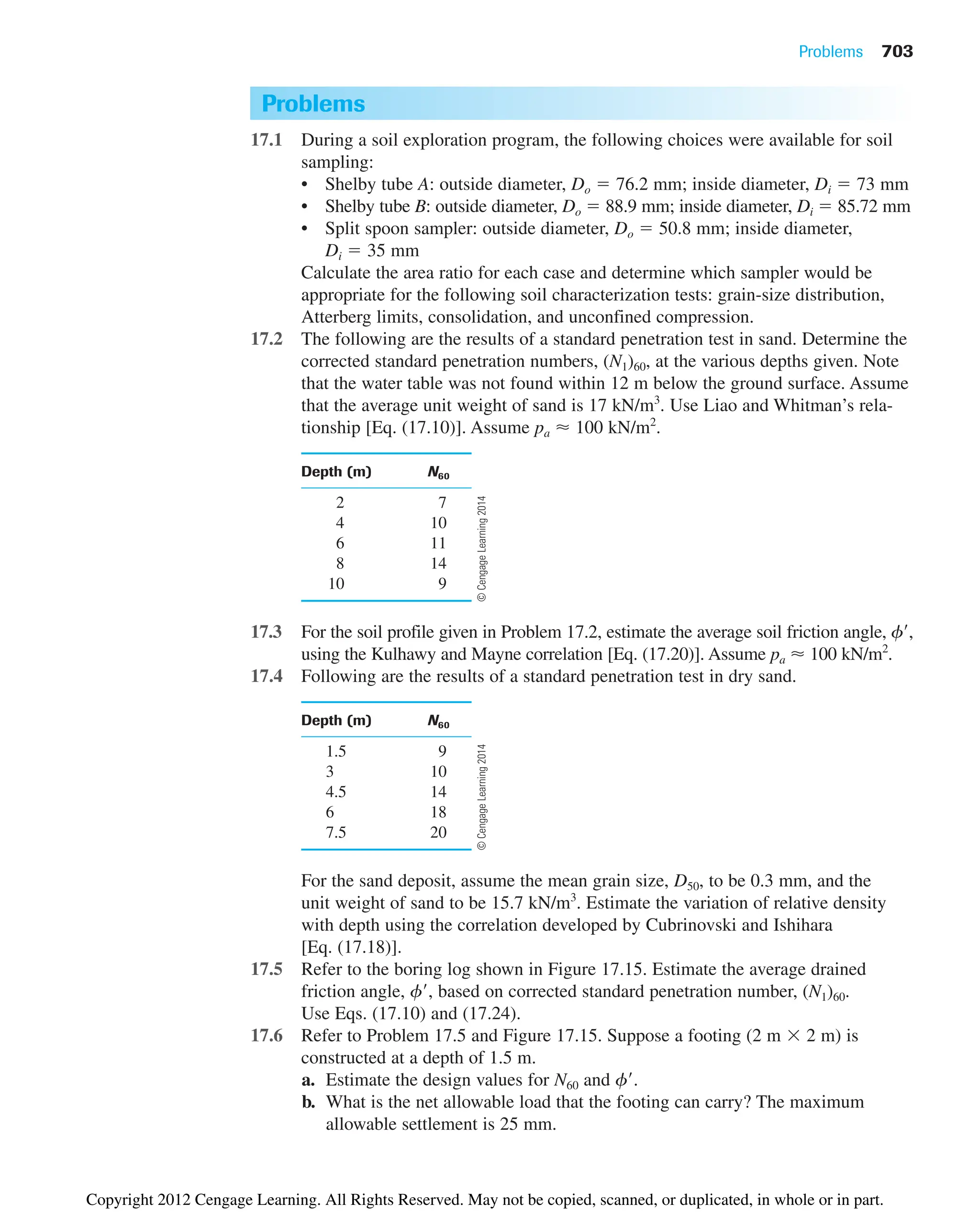
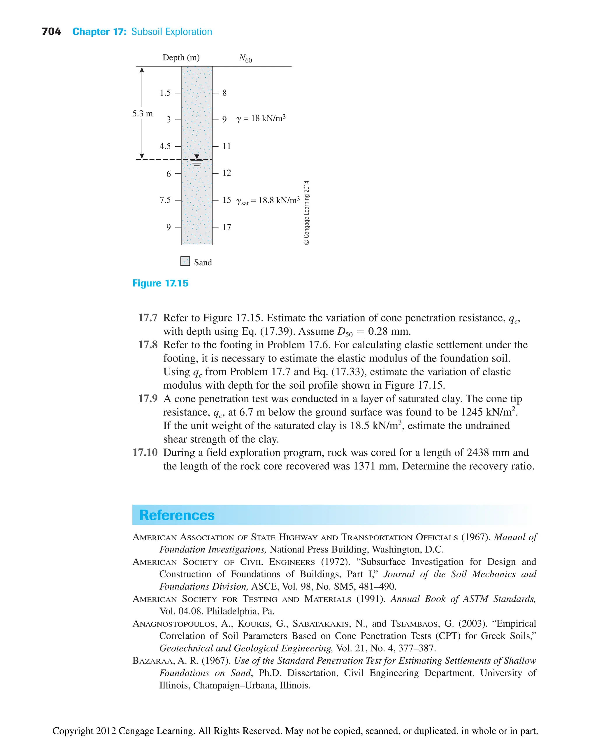
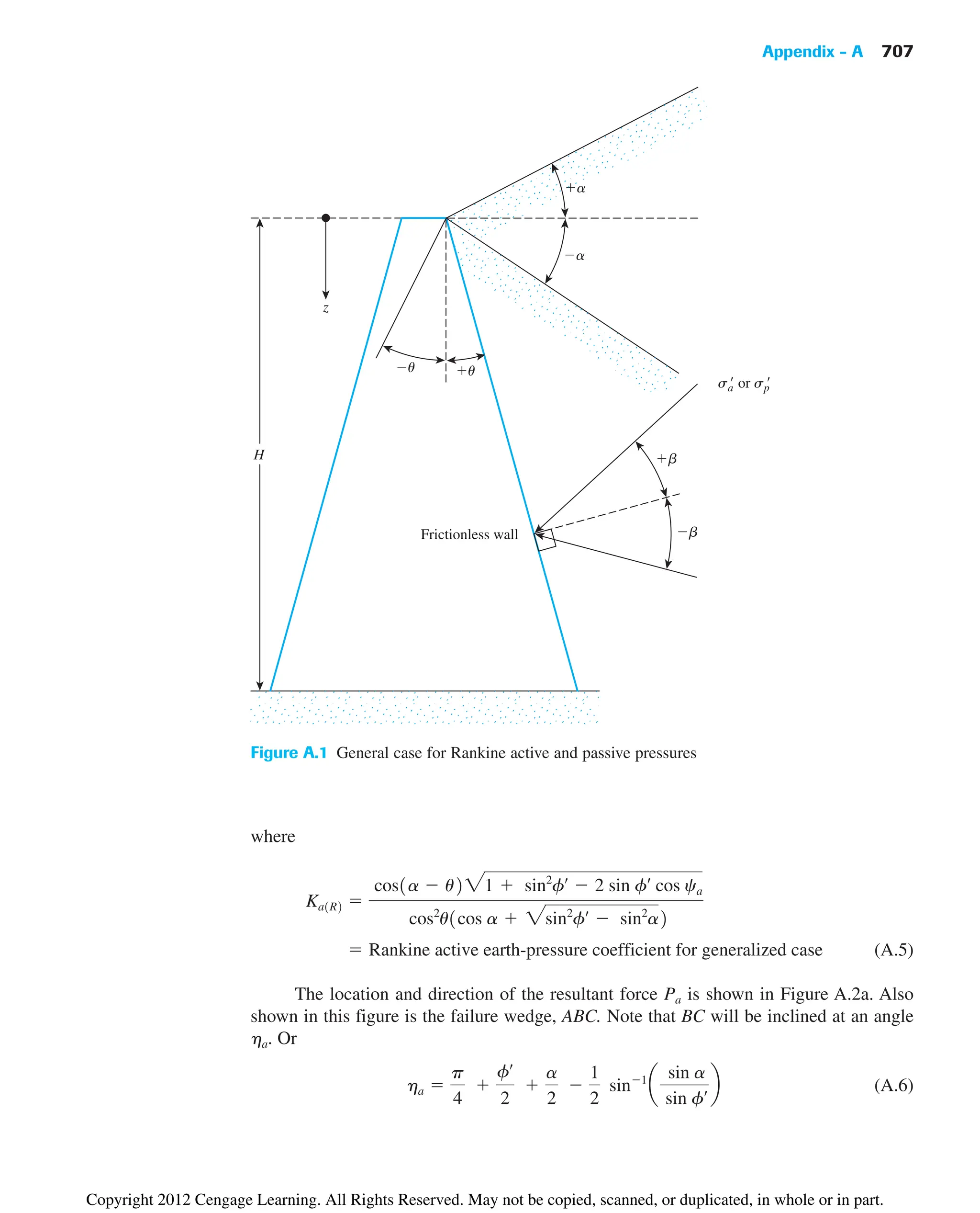
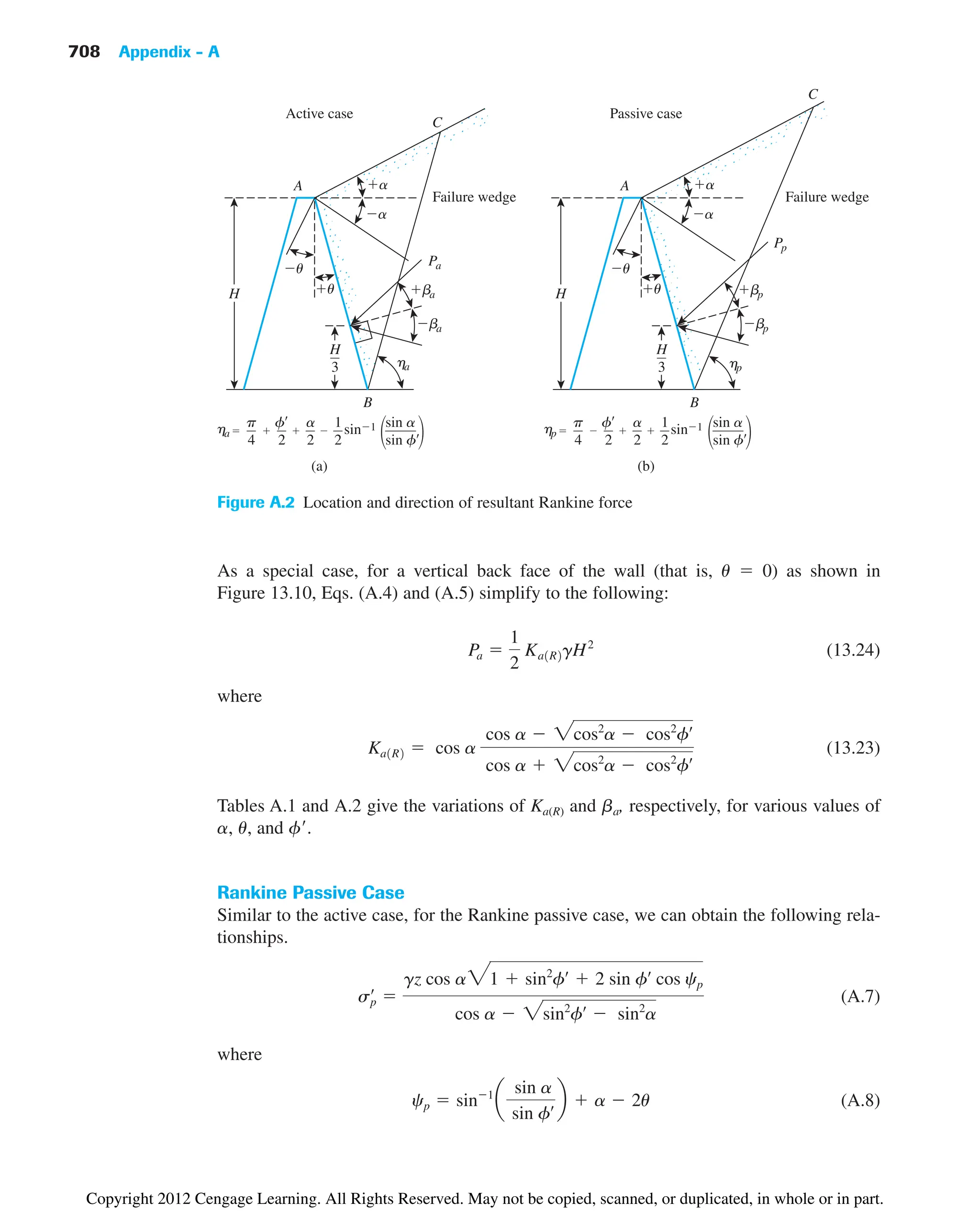
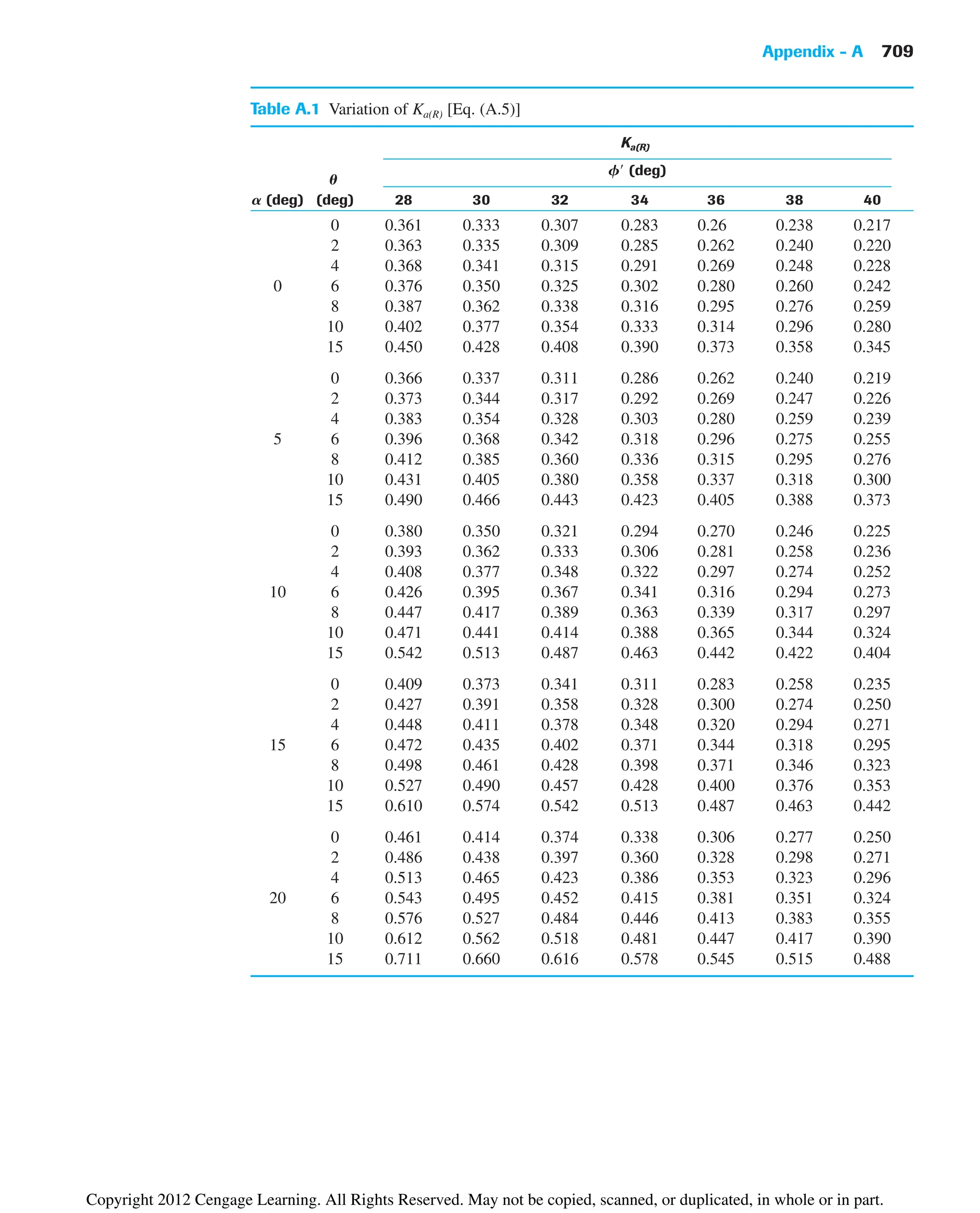
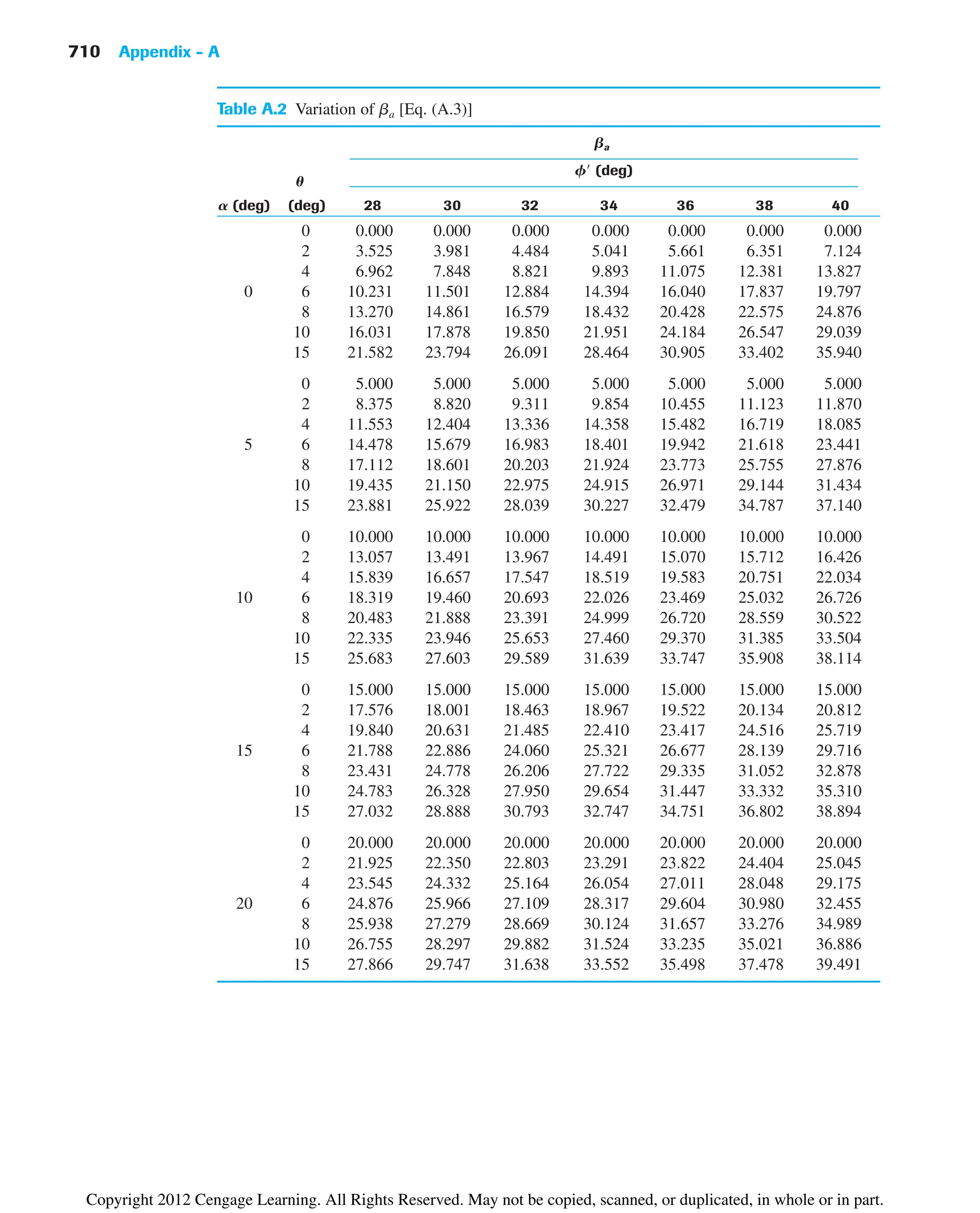
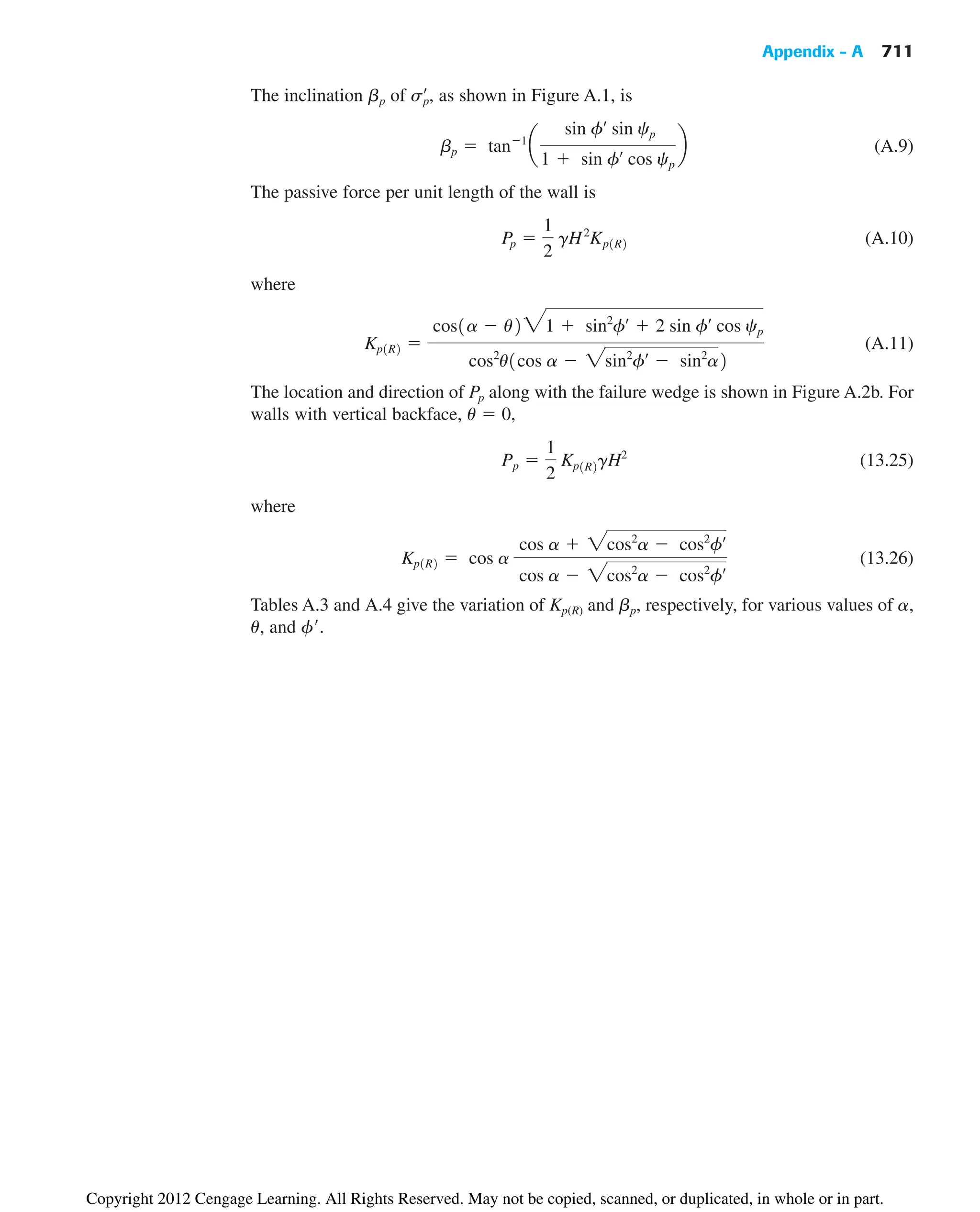
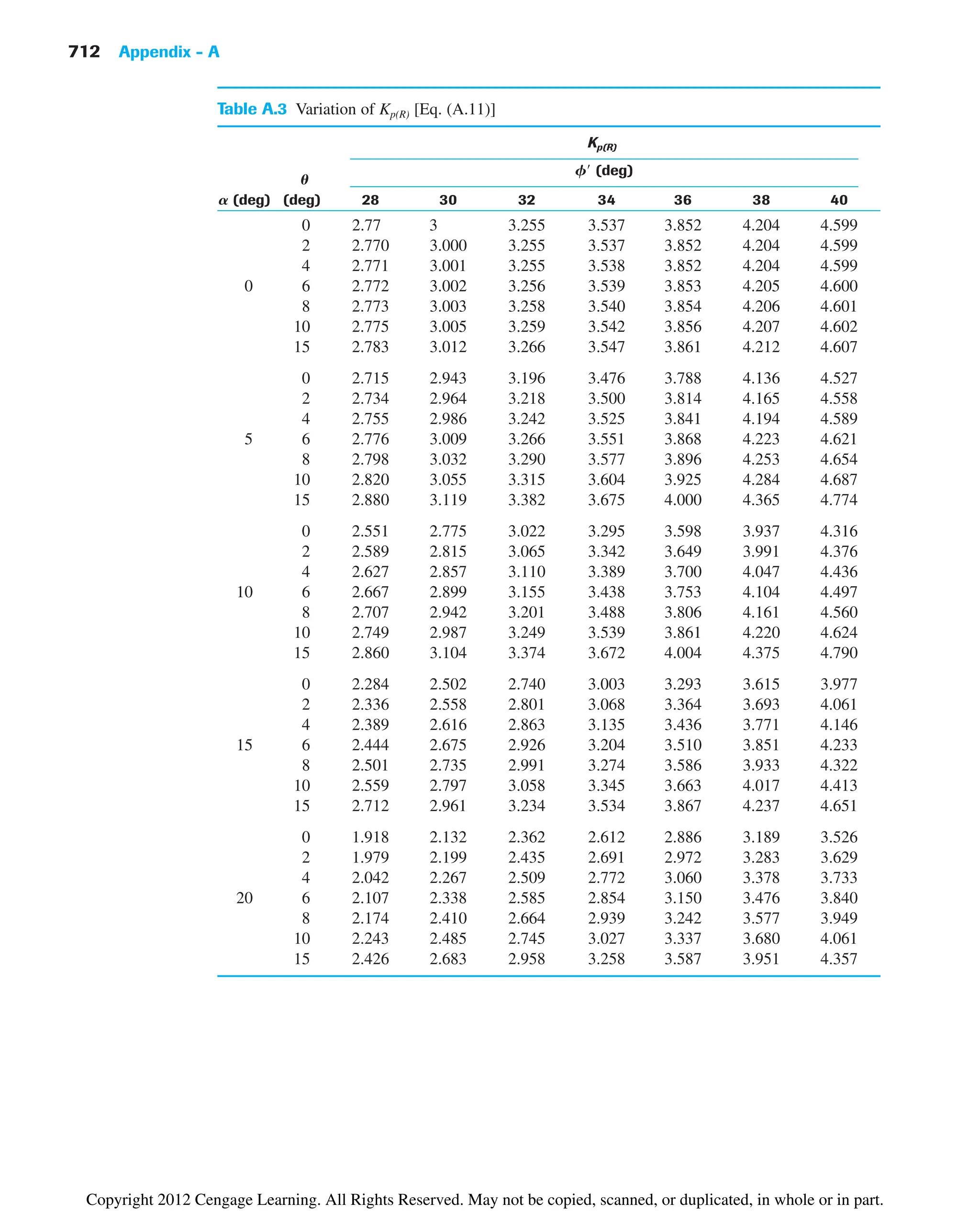
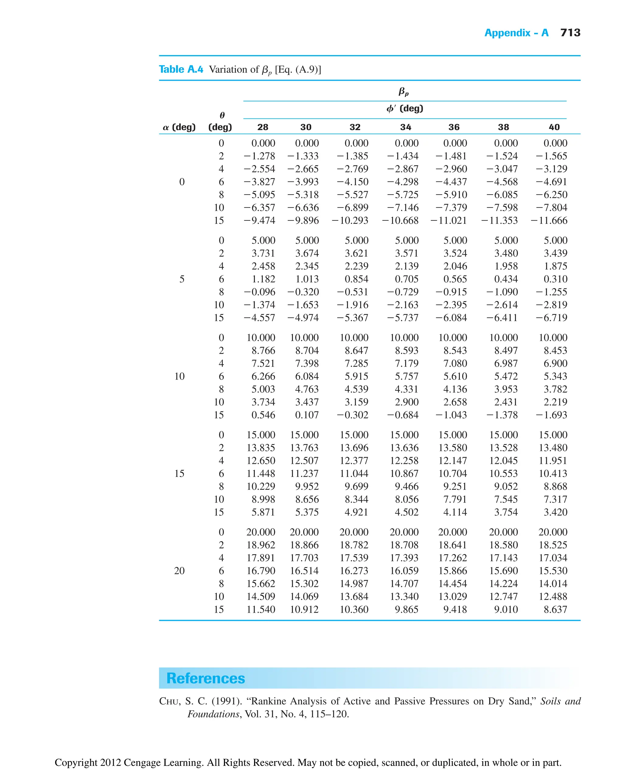
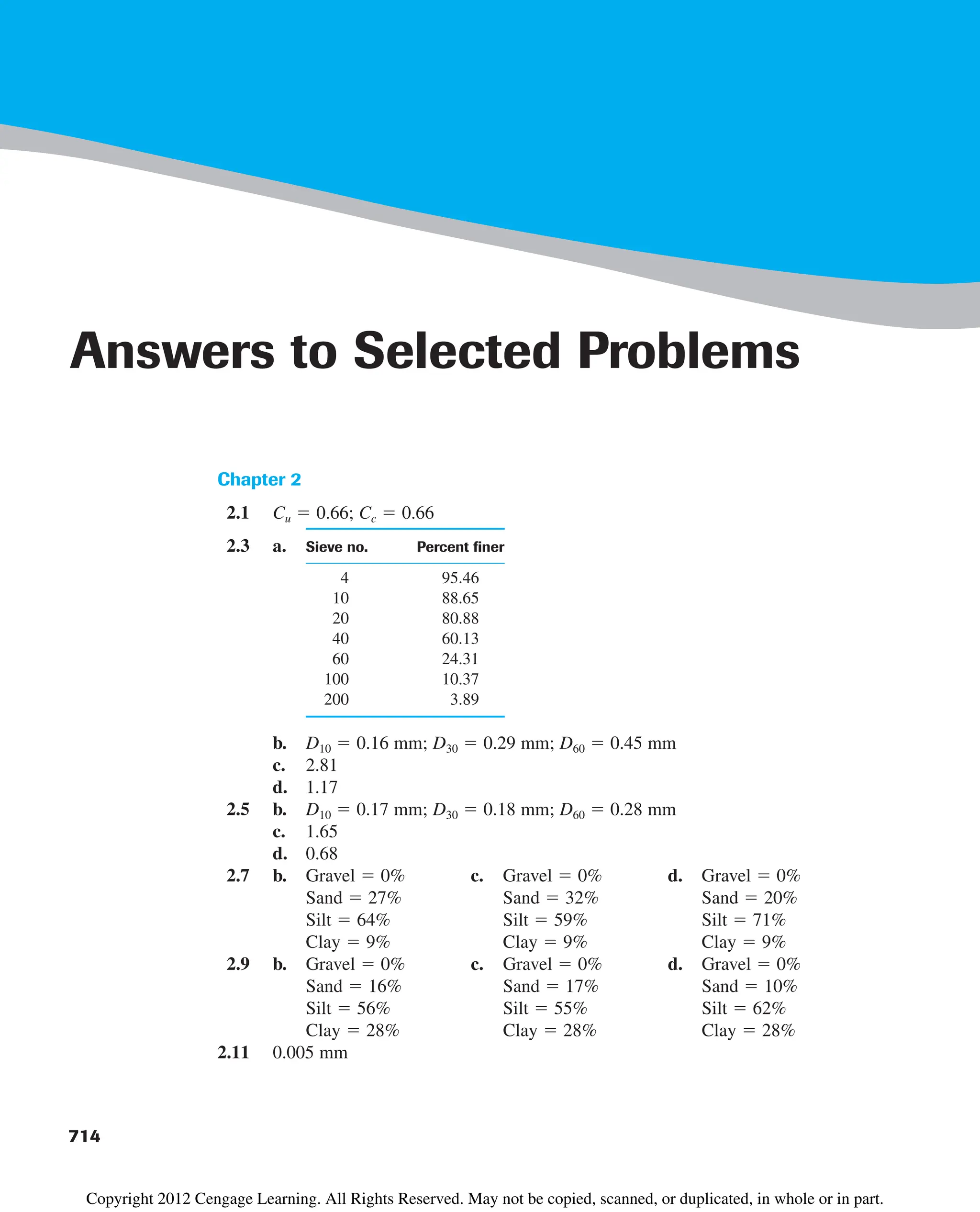
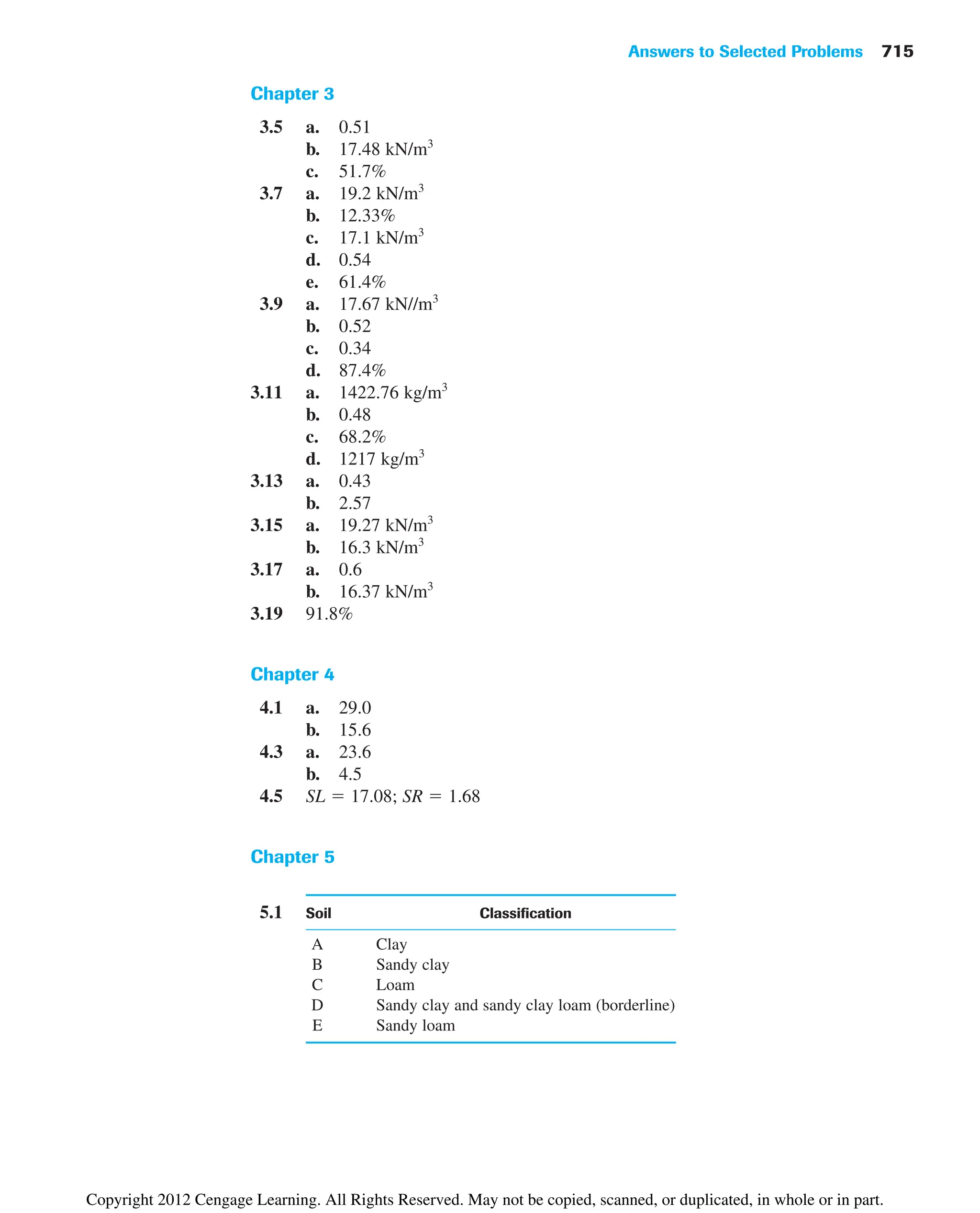
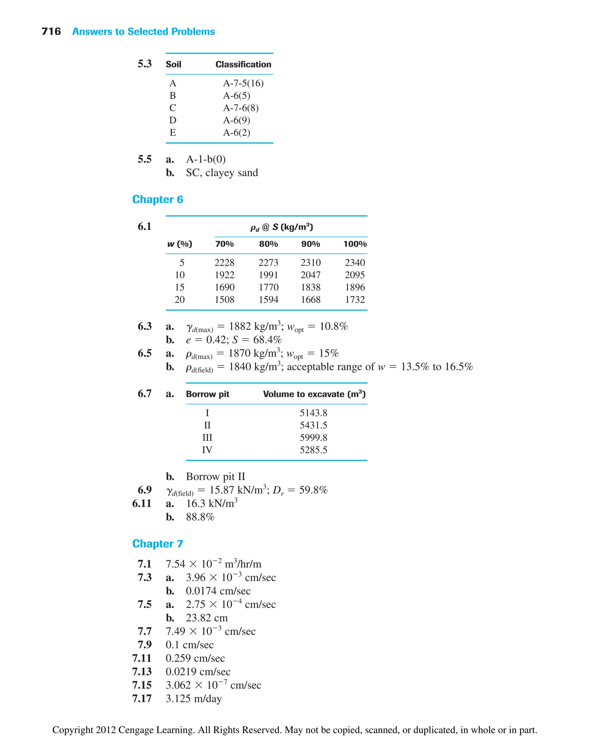
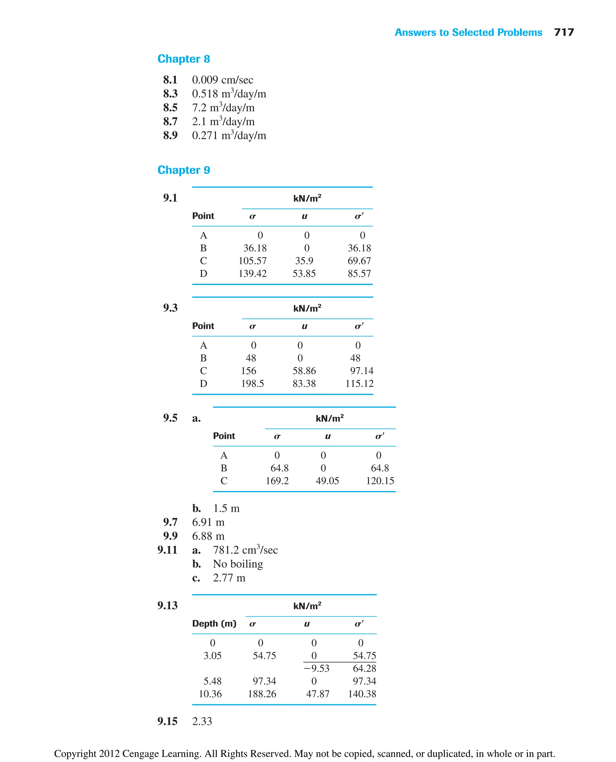
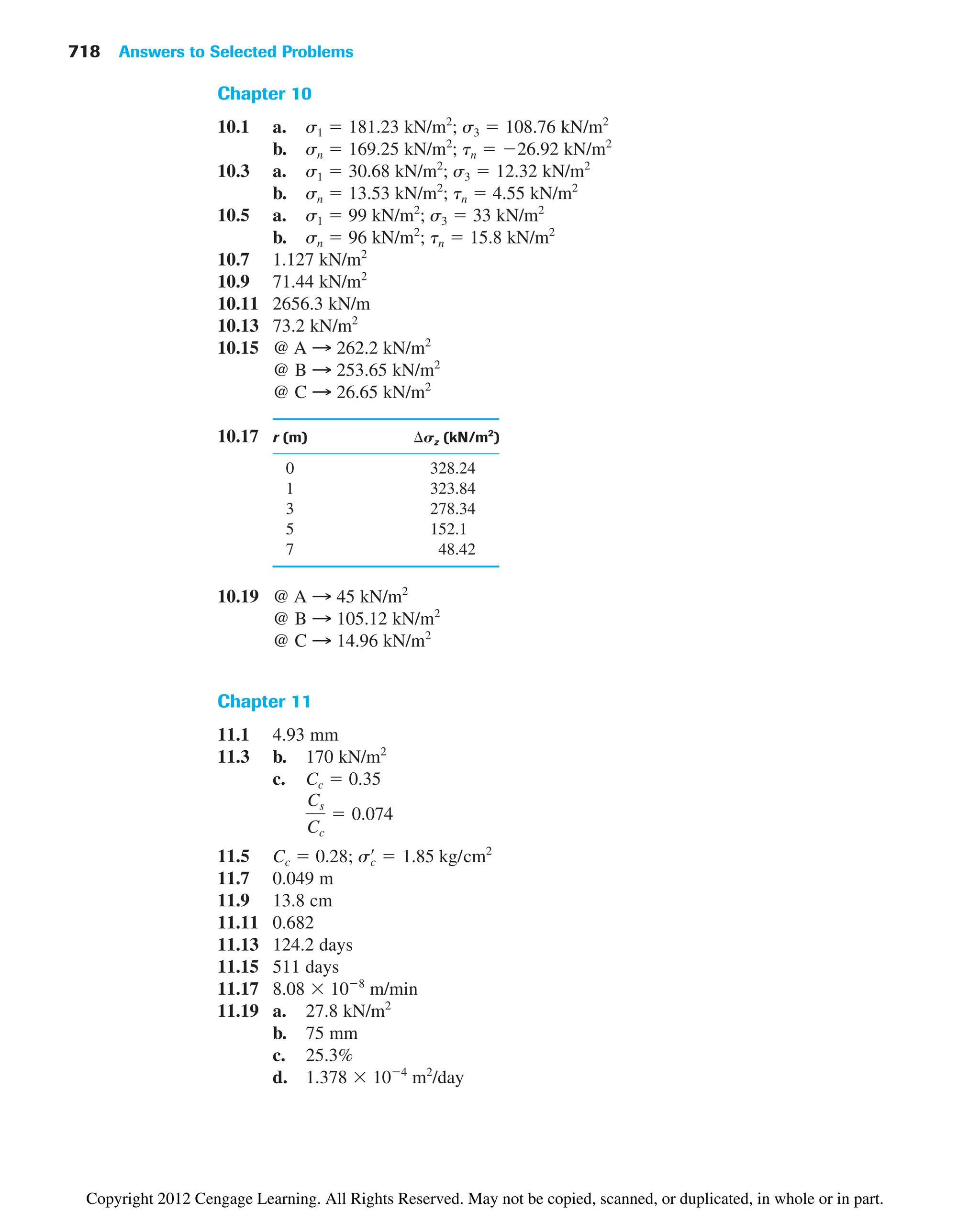
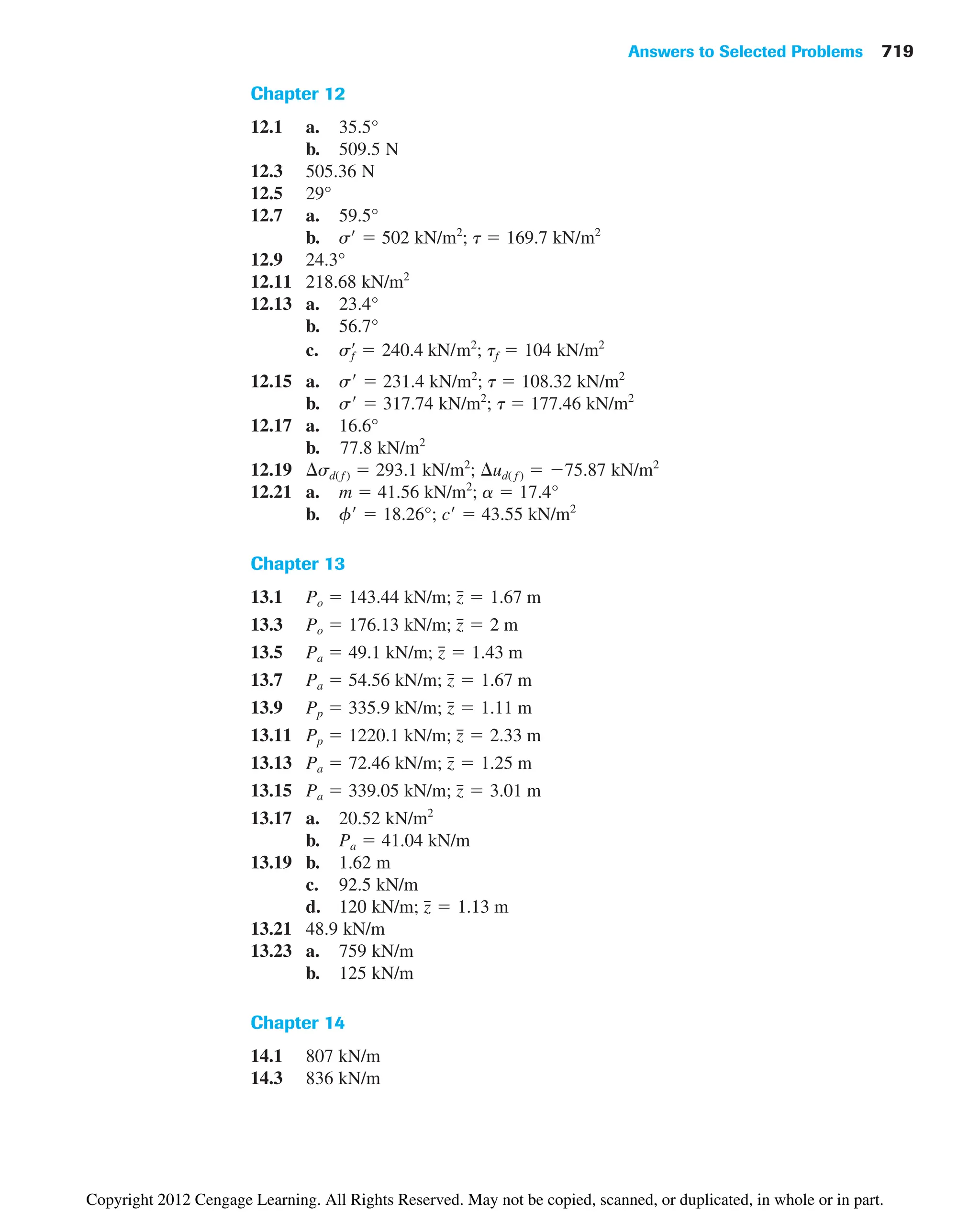
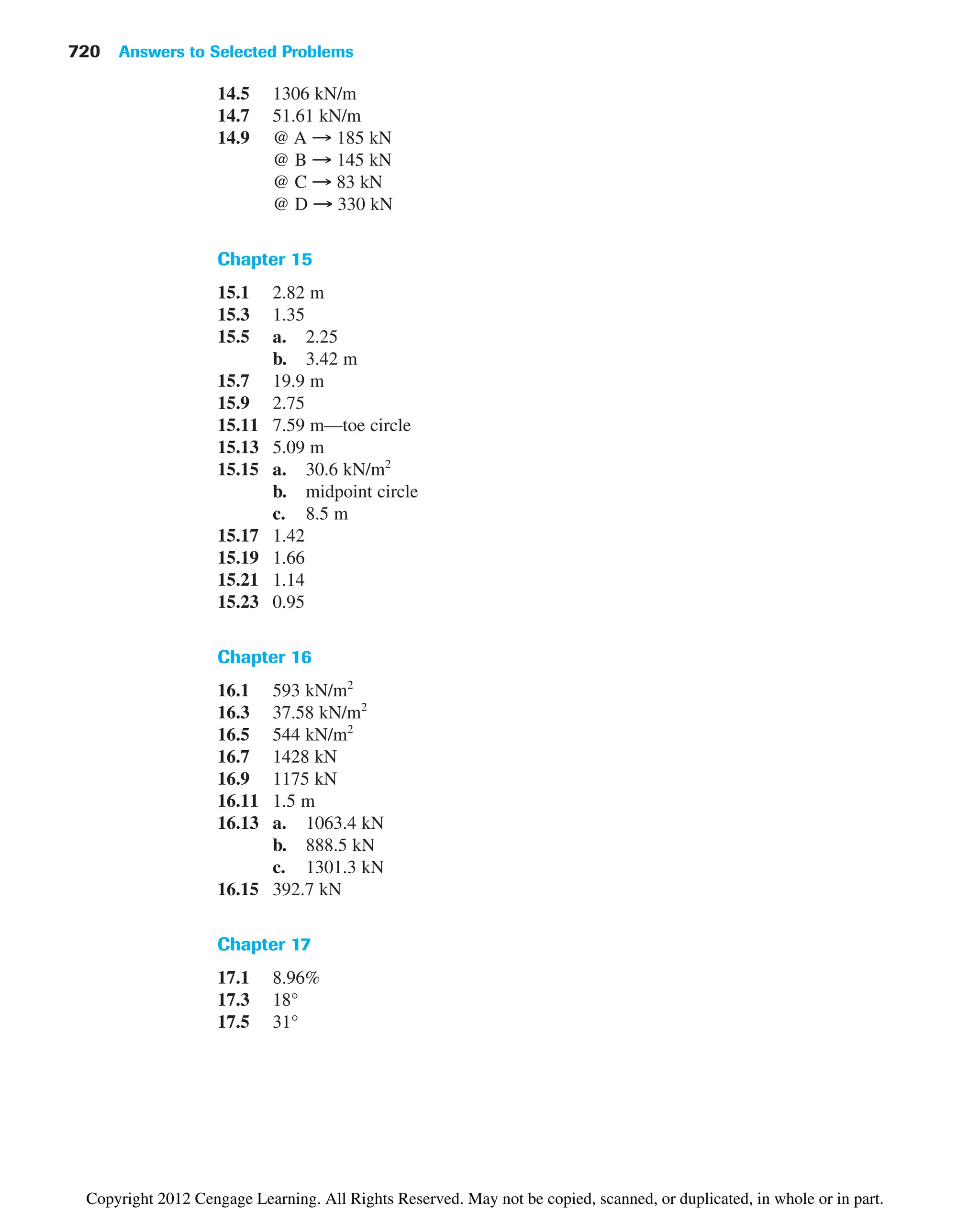
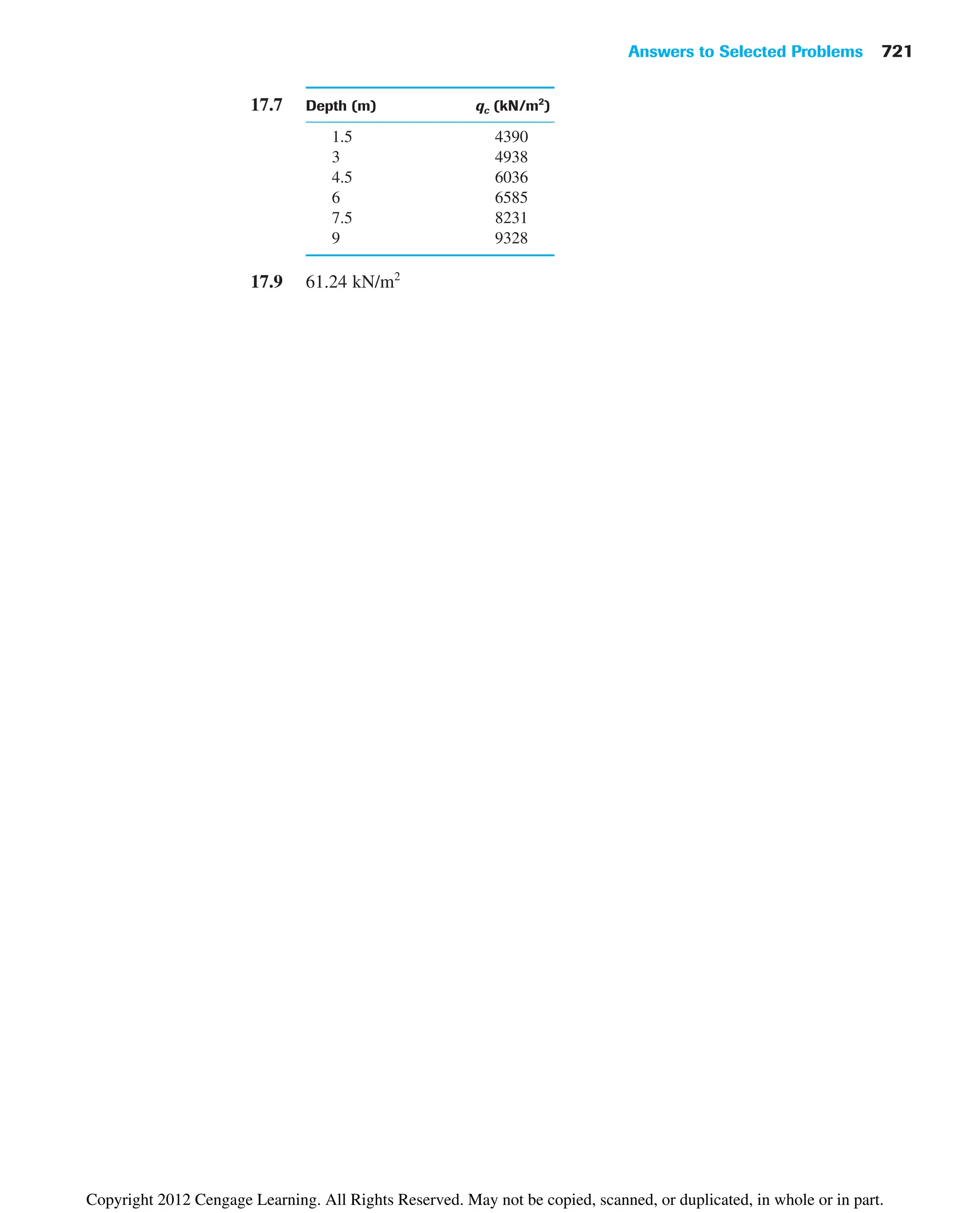


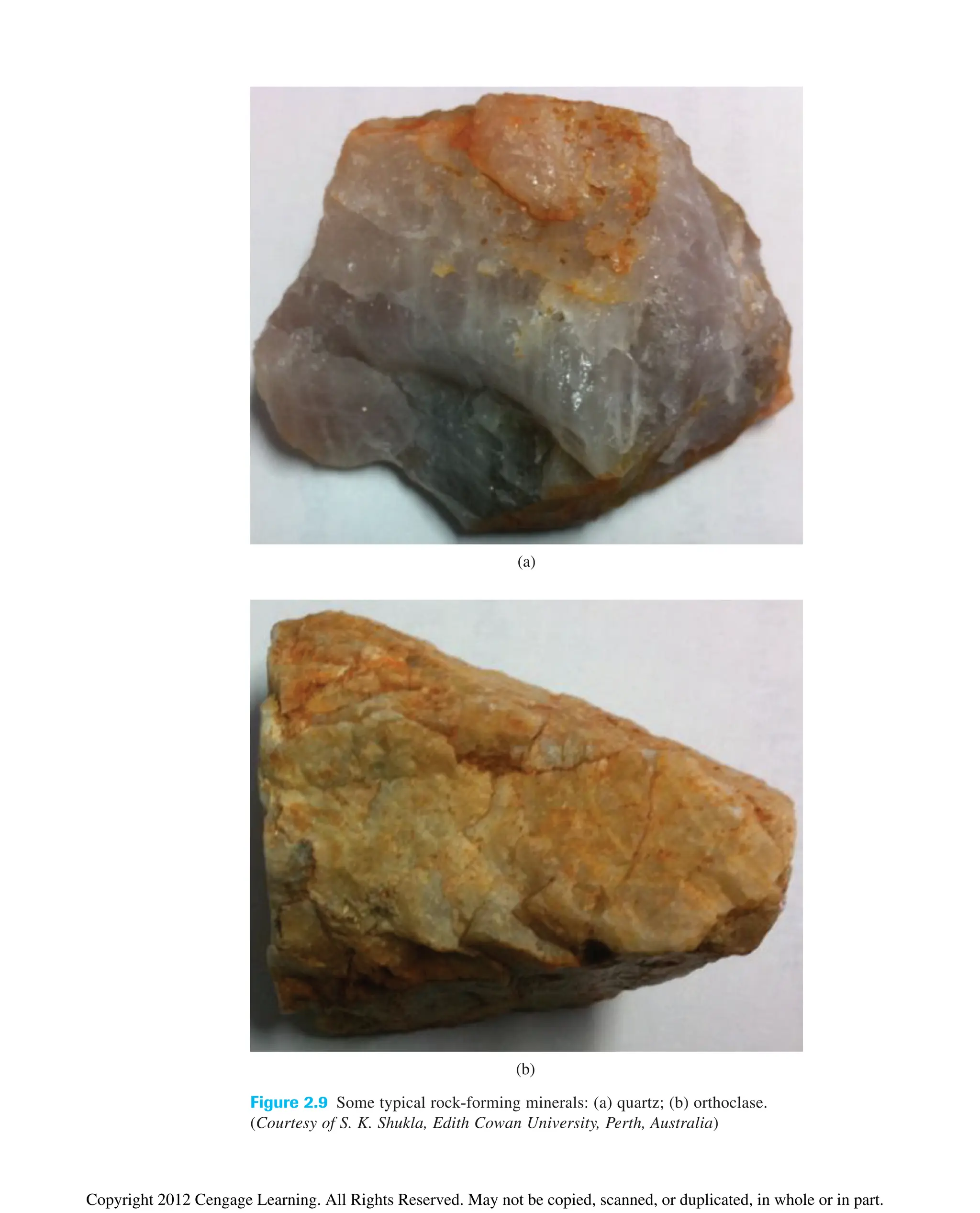
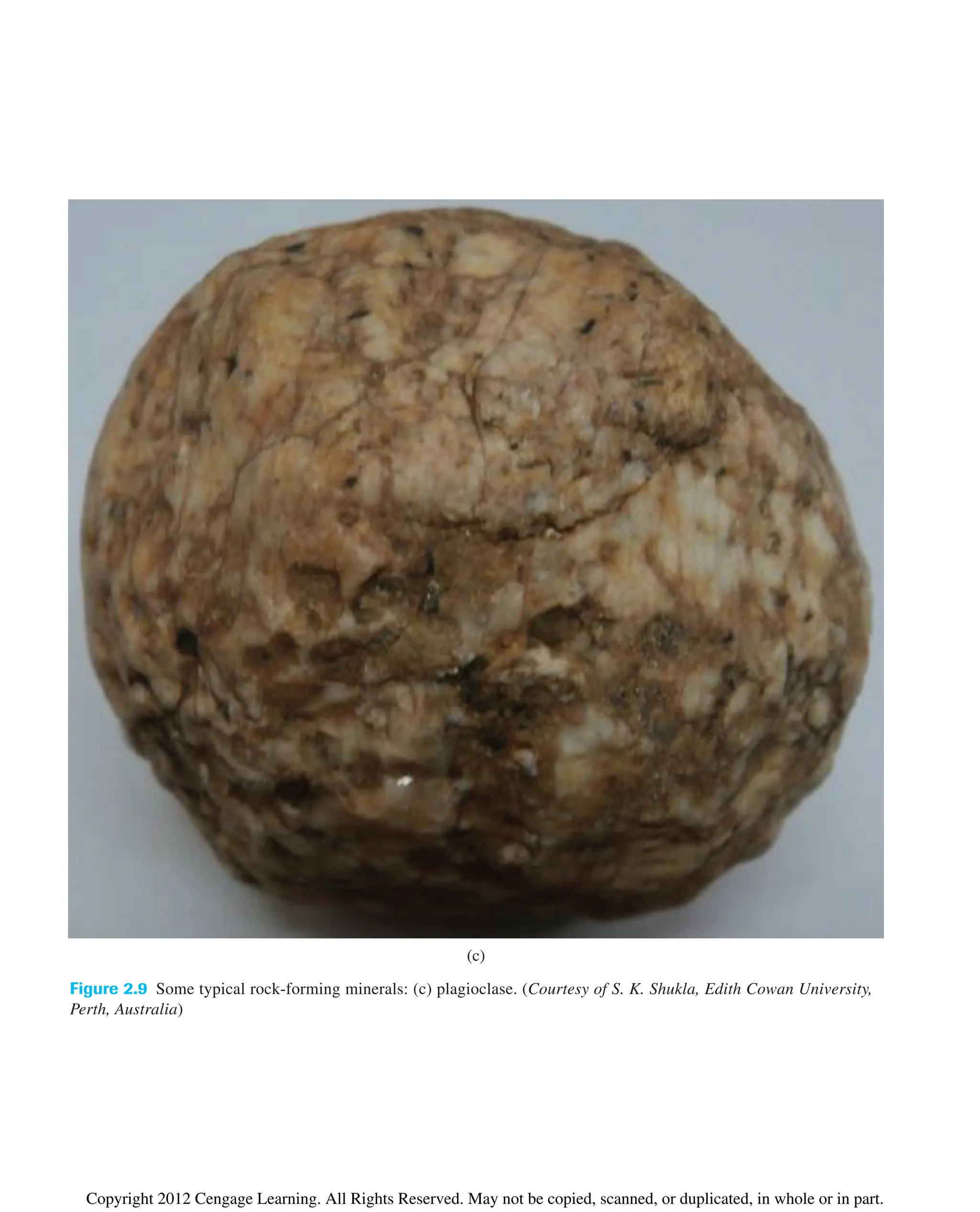
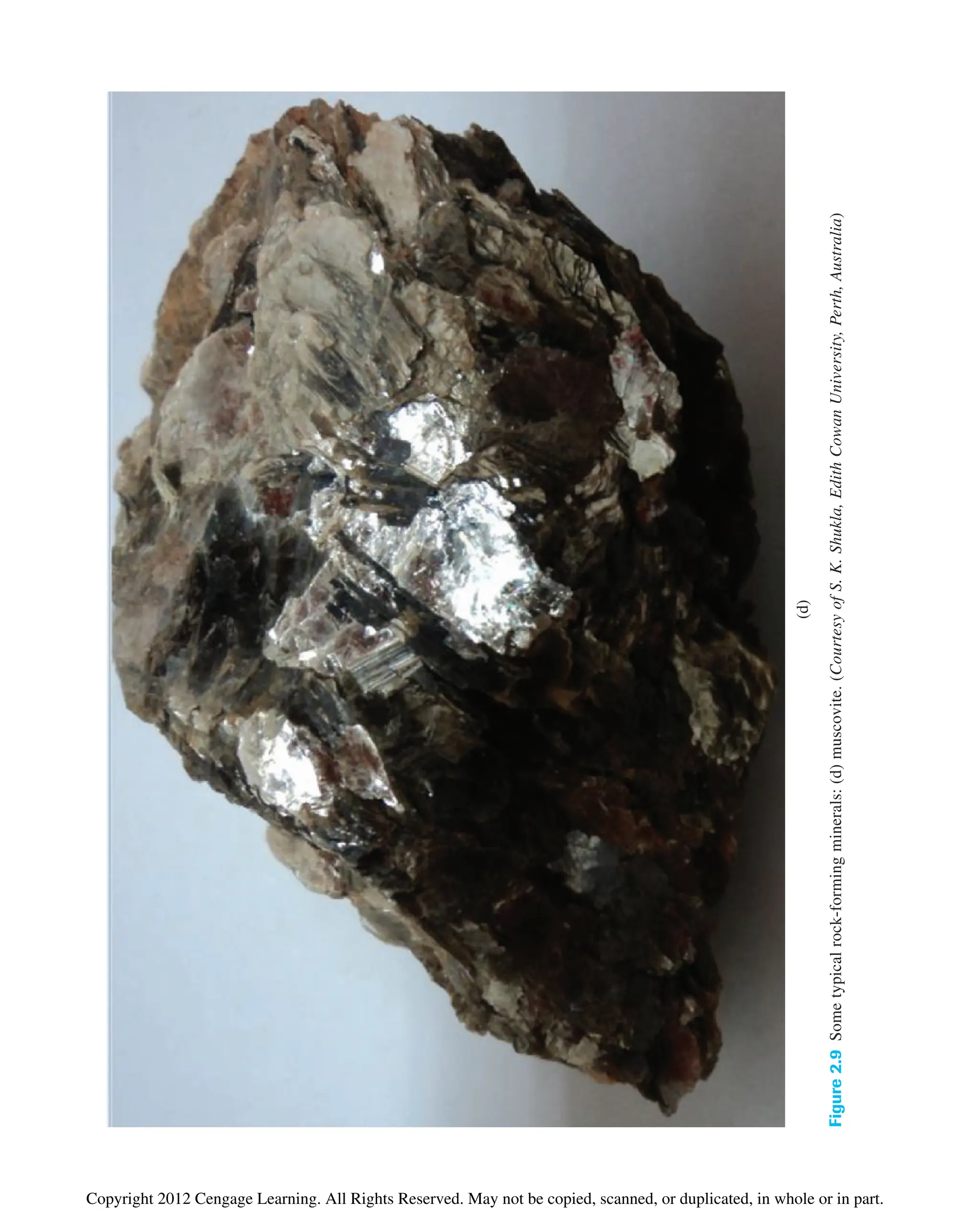
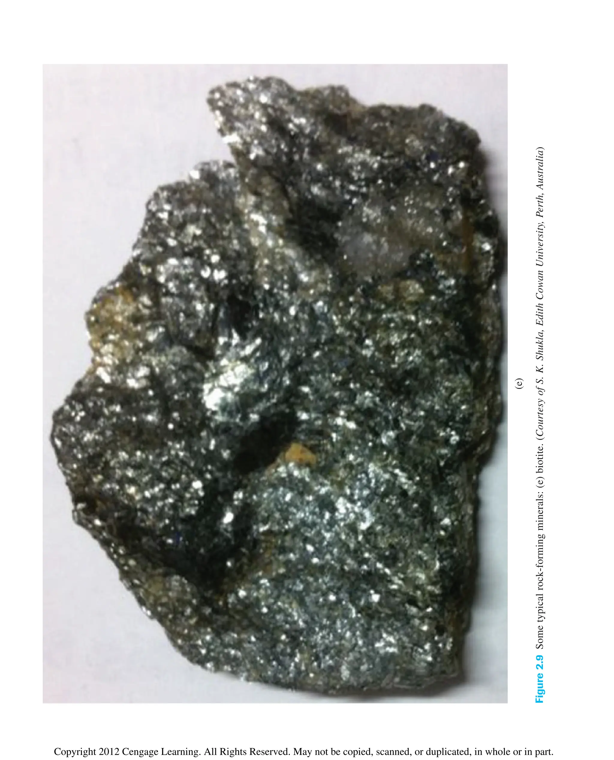
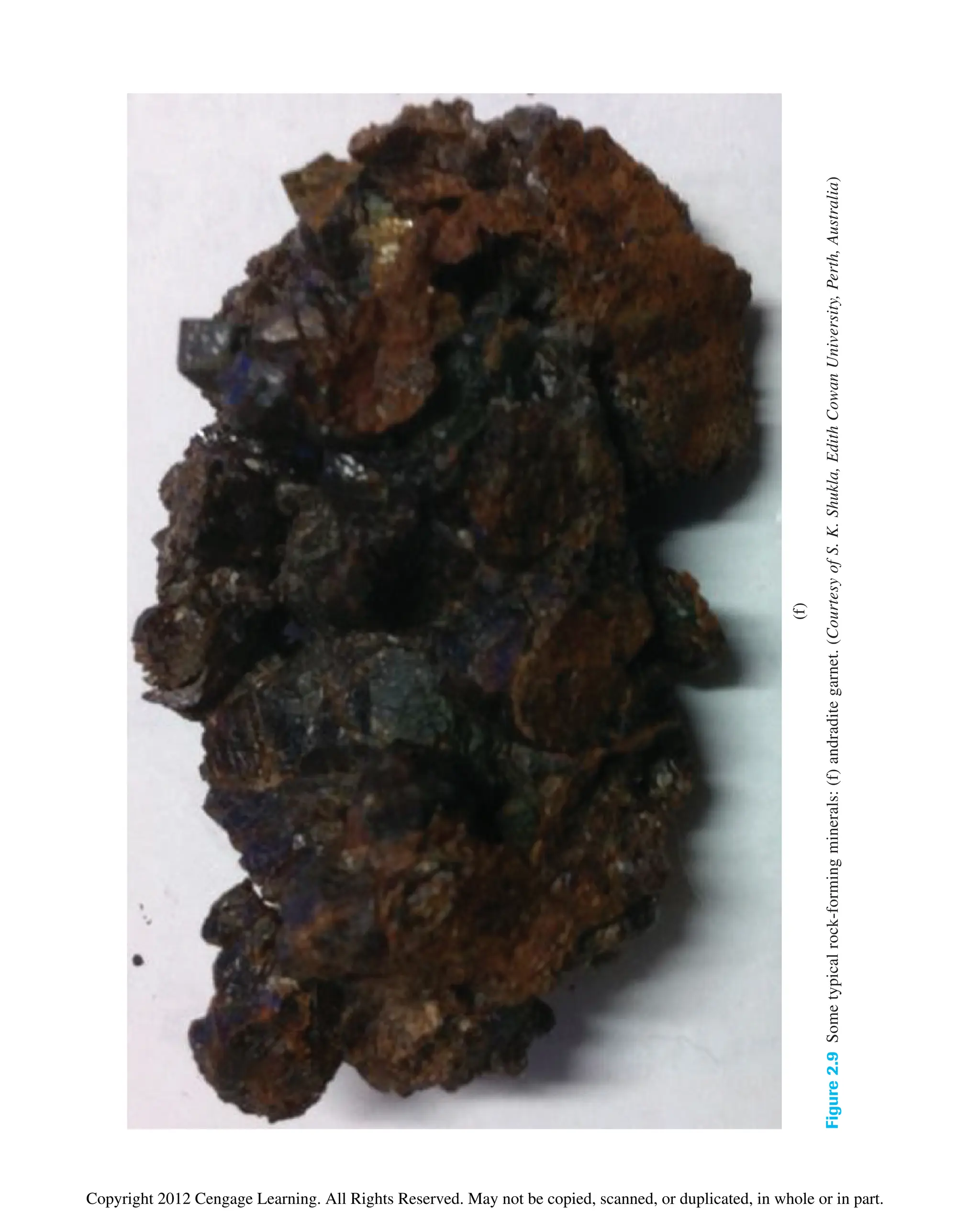
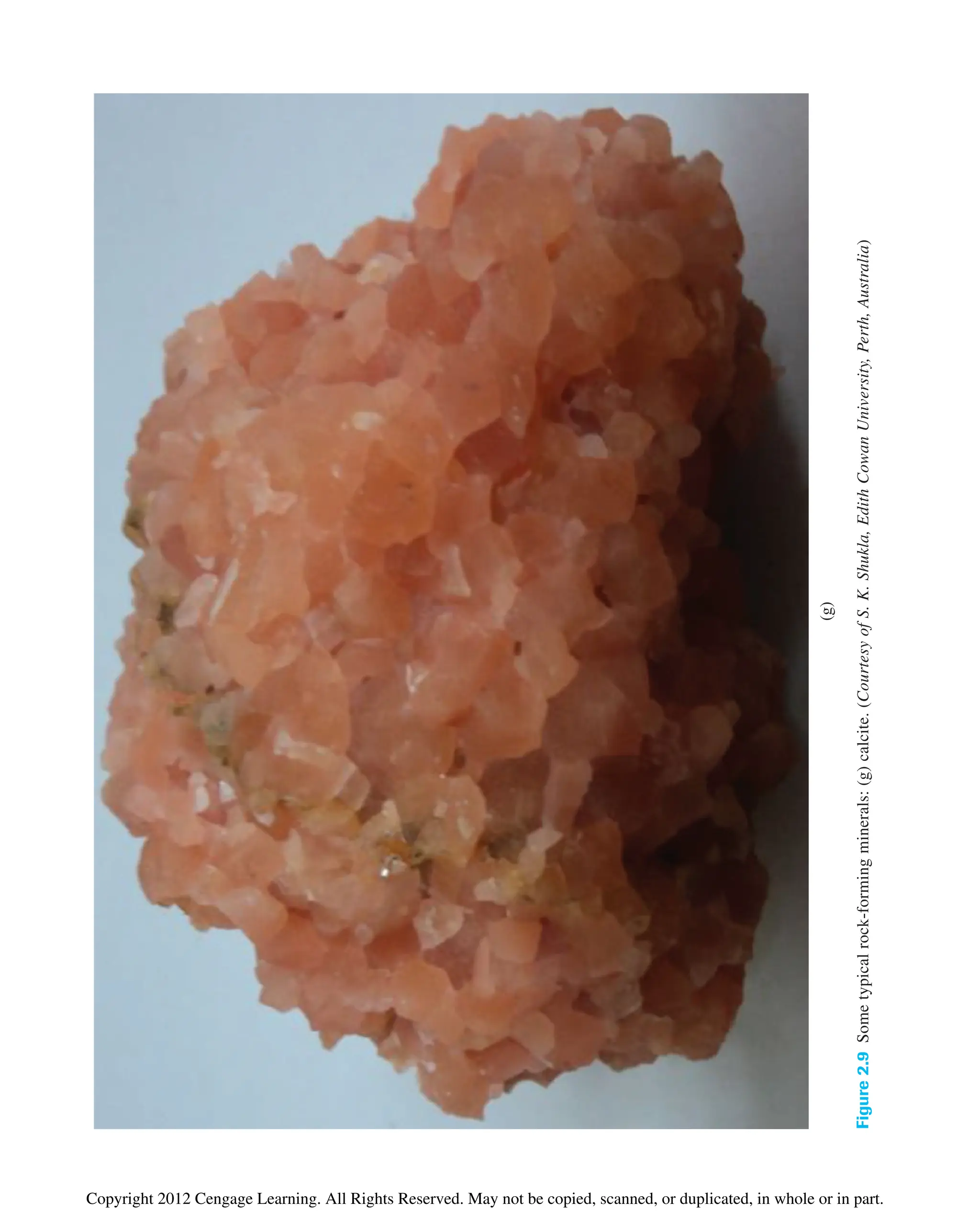
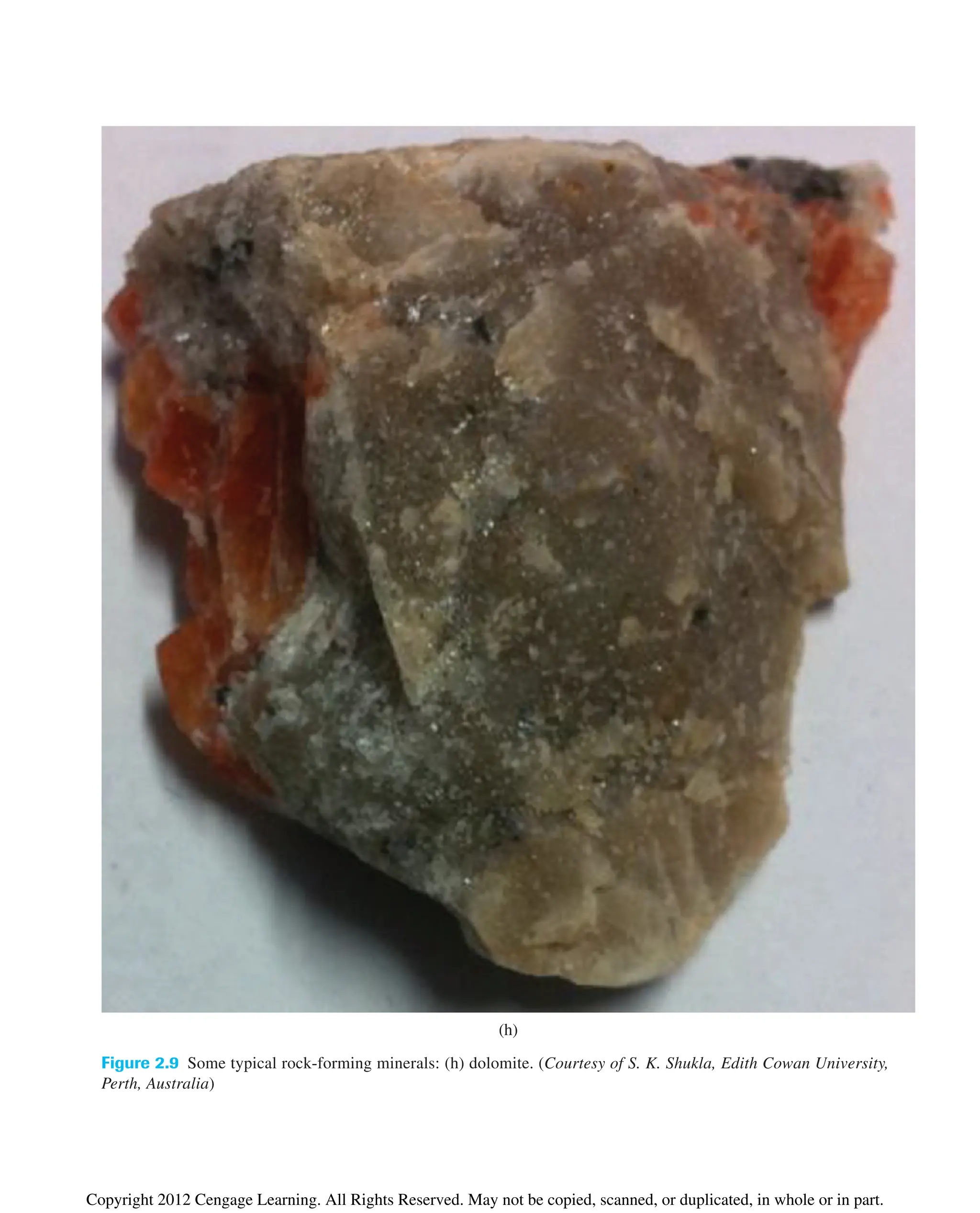
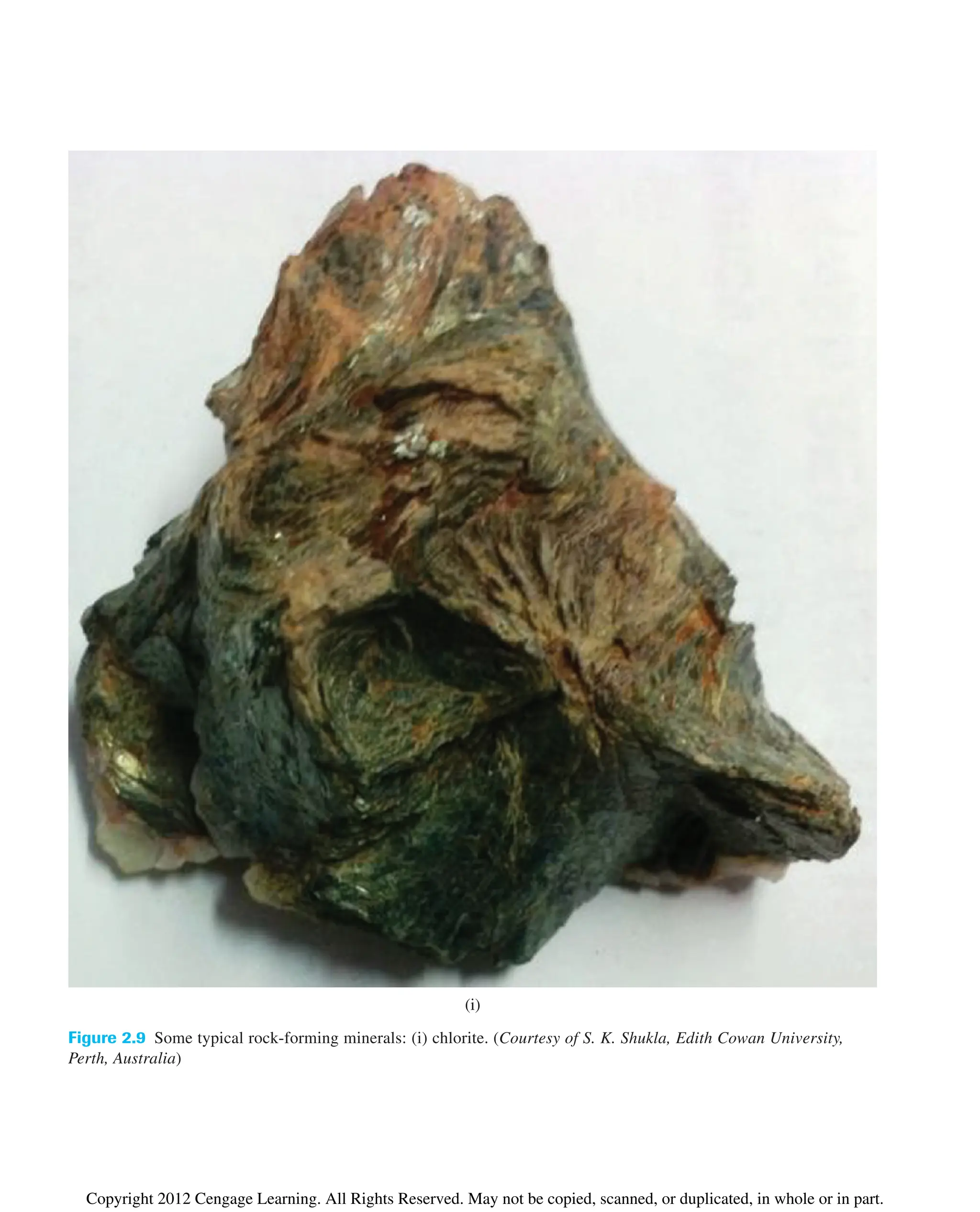
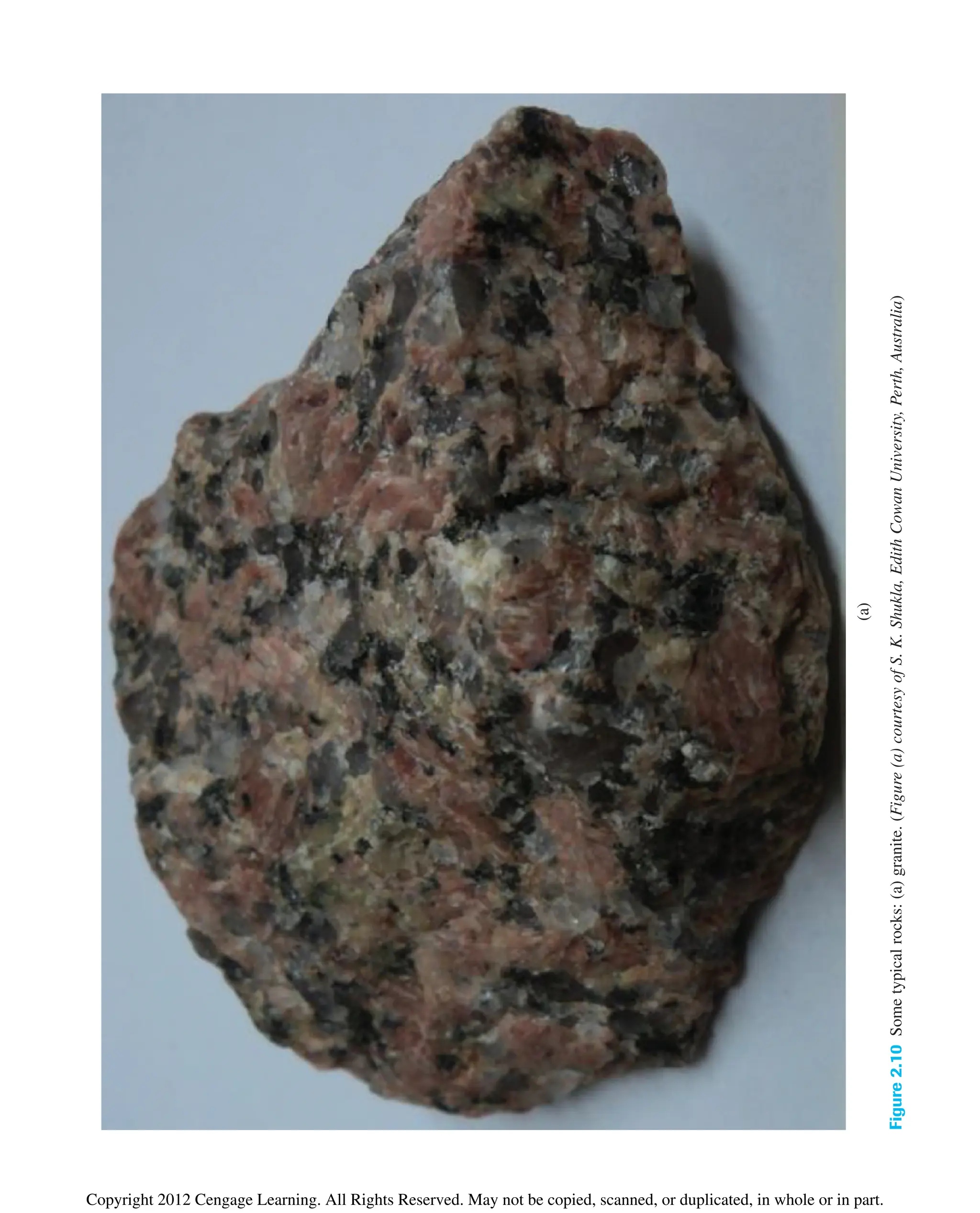
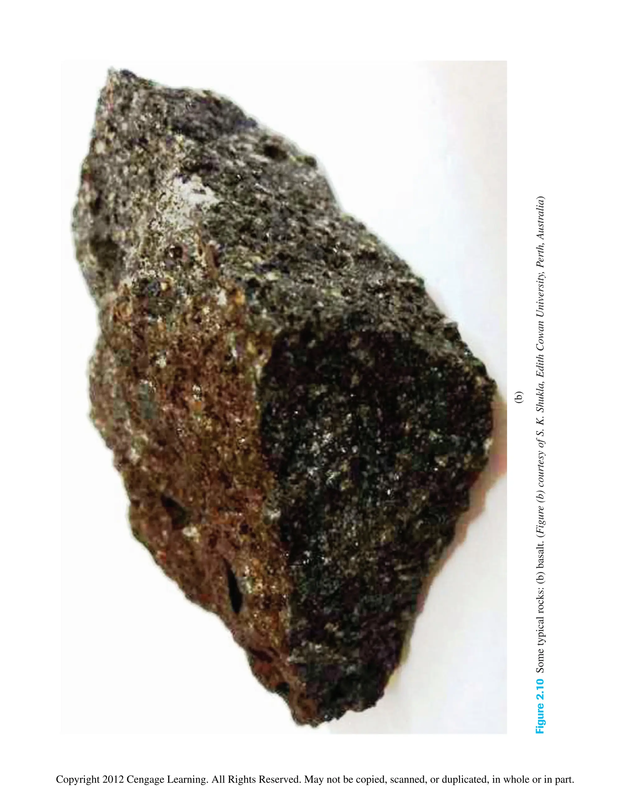
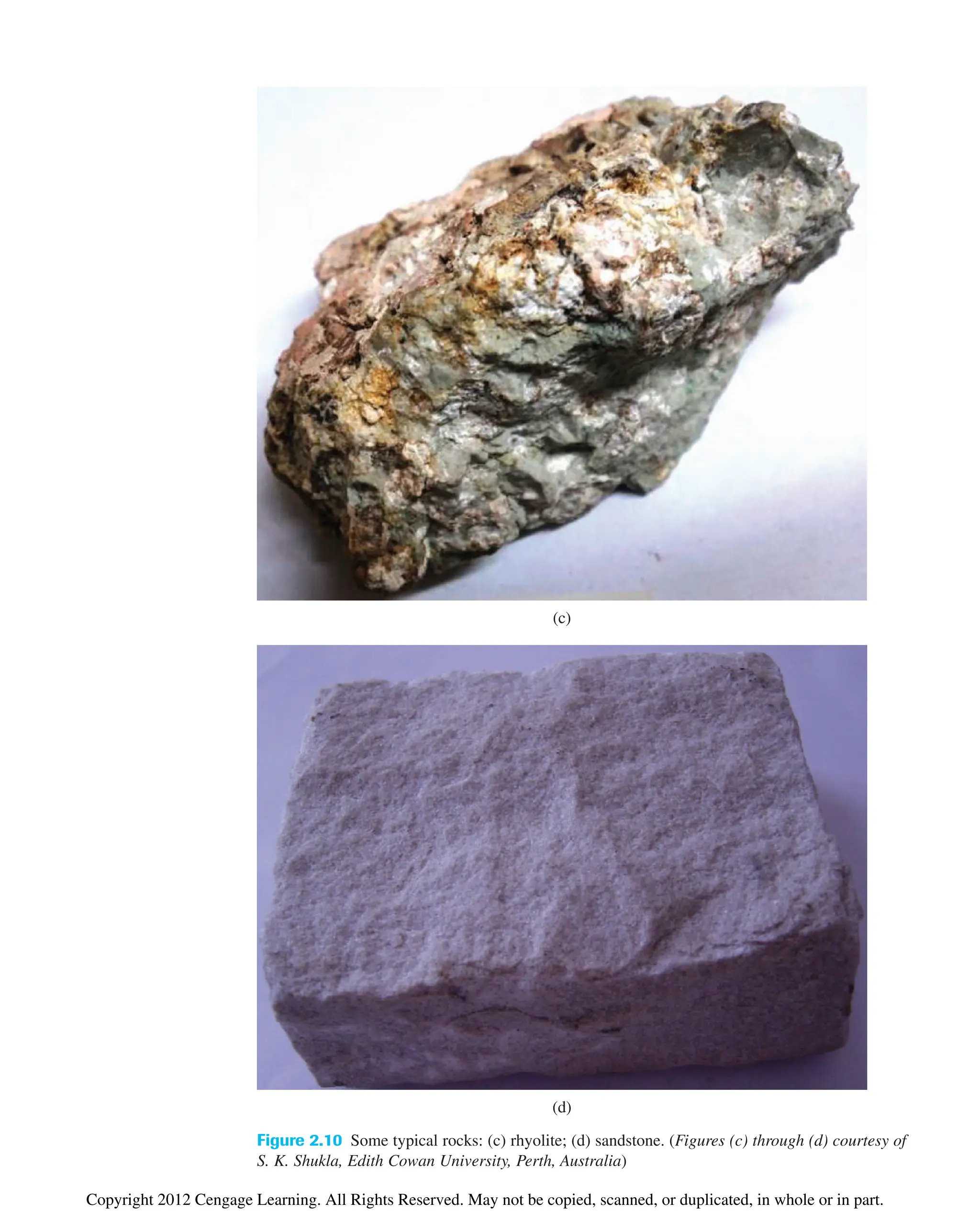
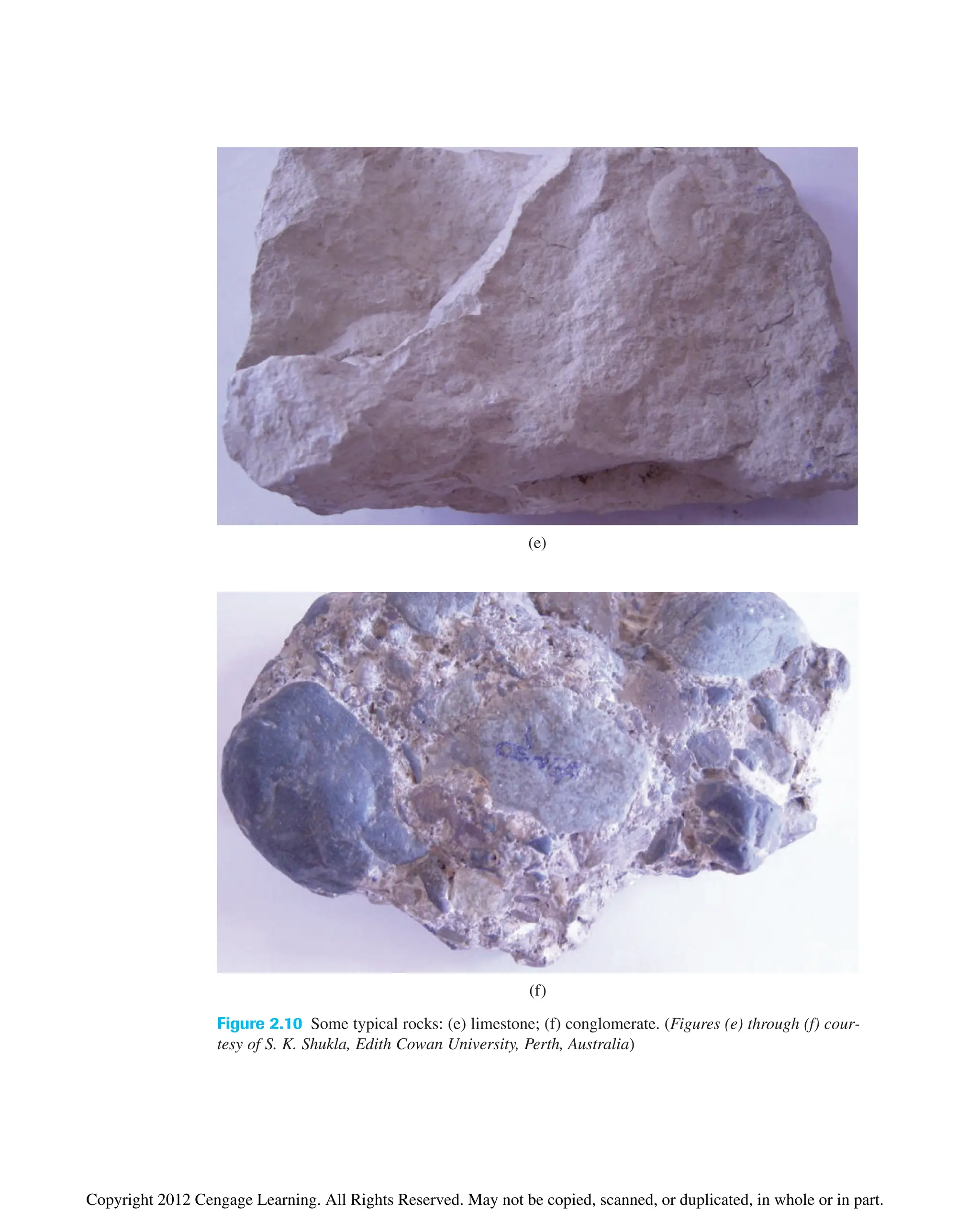
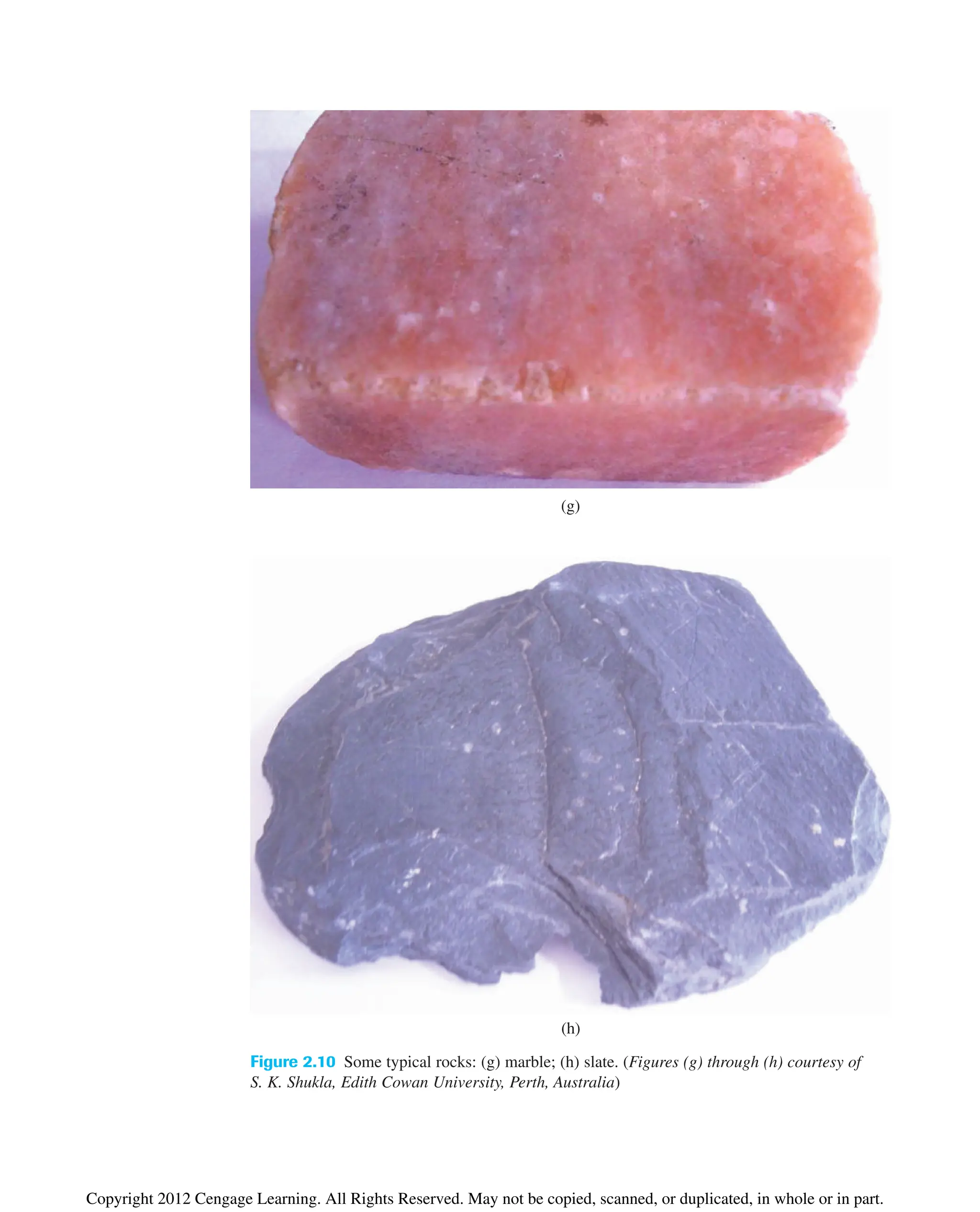
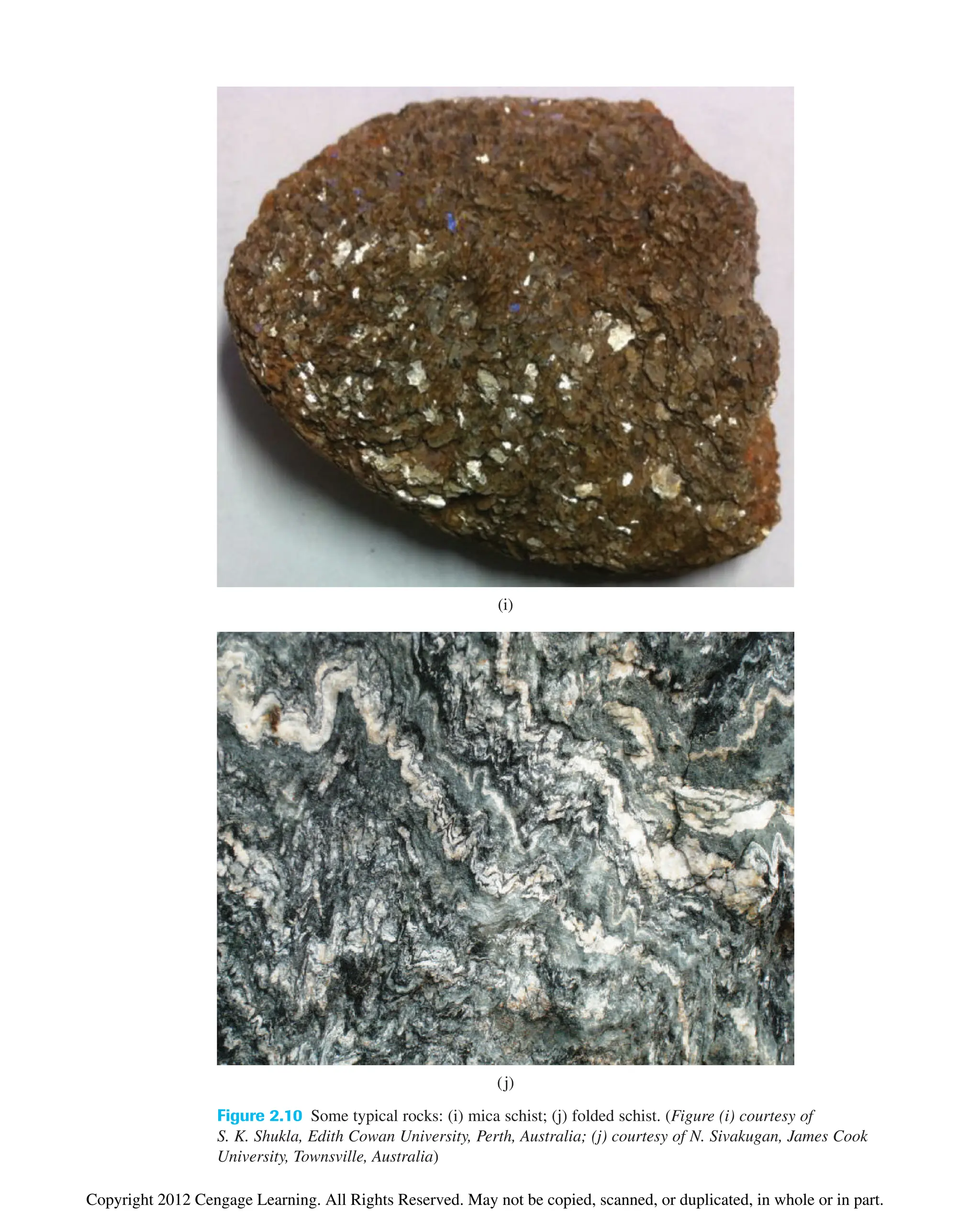
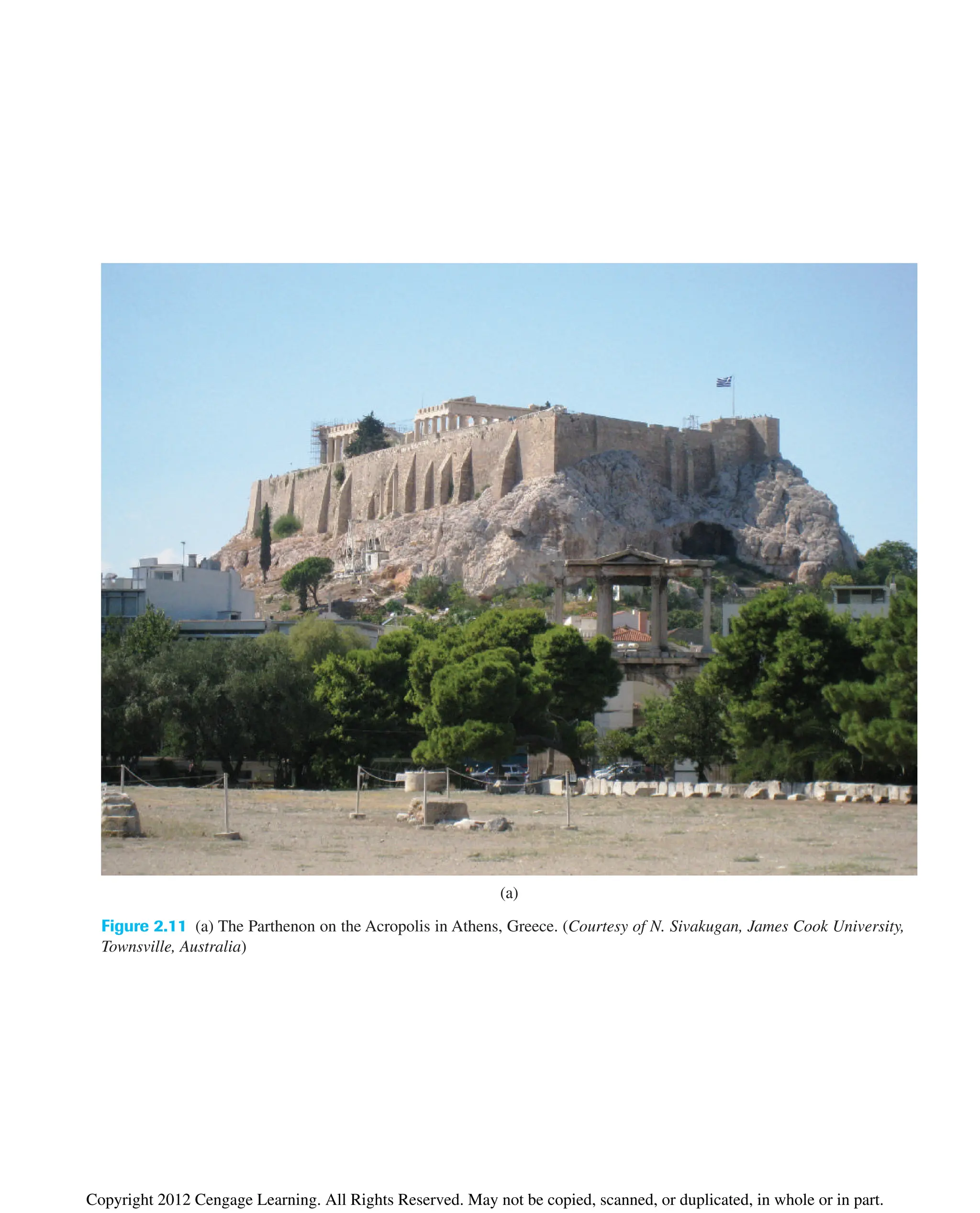
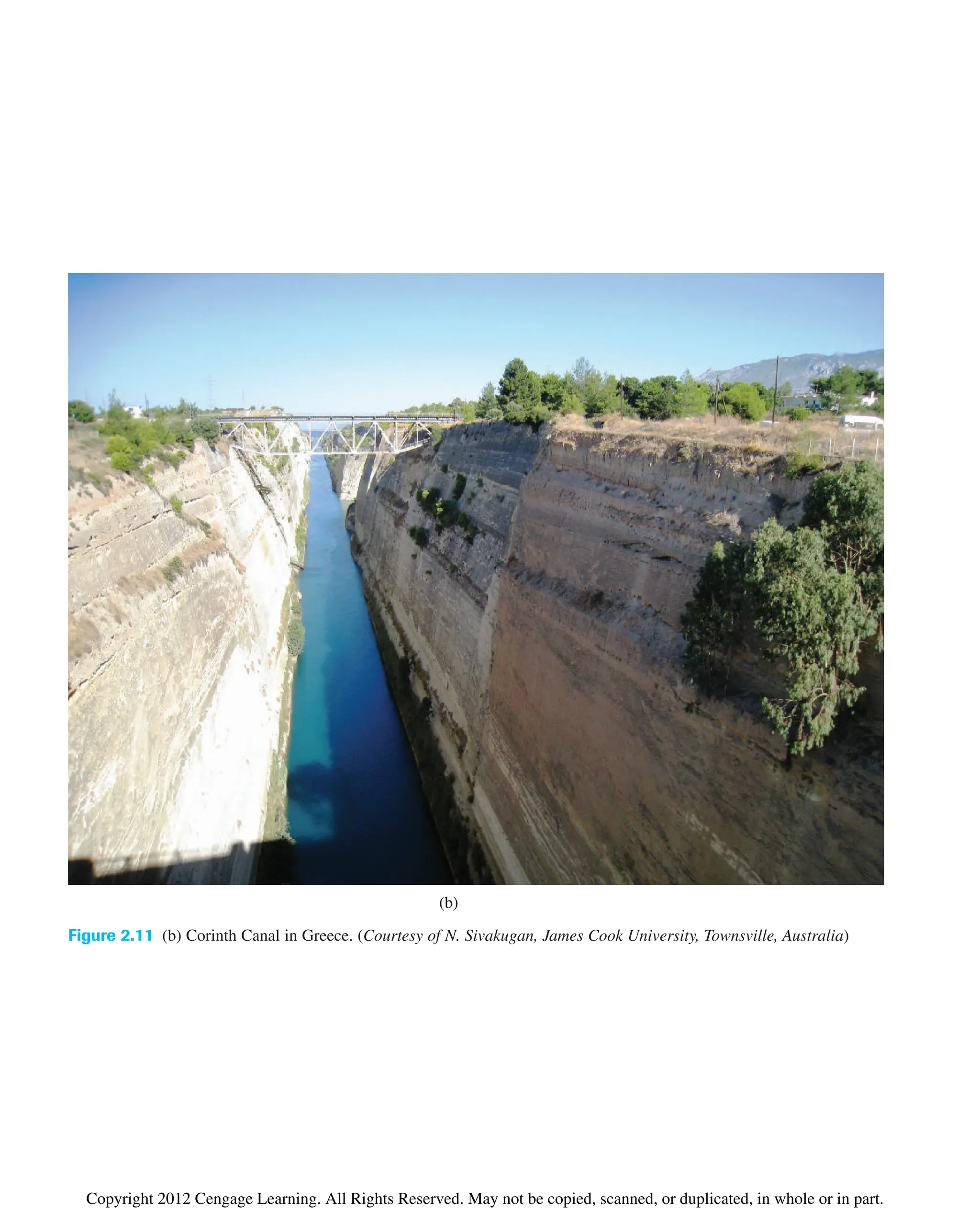


![[Braja m. das]_principles_of_foundation_engineerin(book_fi.org)](https://cdn.slidesharecdn.com/ss_thumbnails/brajam-160923153744-thumbnail.jpg?width=640&height=640&fit=bounds)


![Geotechnical Engineering-I [Lec #9: Atterberg limits]](https://cdn.slidesharecdn.com/ss_thumbnails/9-180923180923-thumbnail.jpg?width=640&height=640&fit=bounds)


![Geotechnical Engineering-I [Lec #24: Soil Permeability - II]](https://cdn.slidesharecdn.com/ss_thumbnails/24-180924141149-thumbnail.jpg?width=640&height=640&fit=bounds)


![Geotechnical Engineering-I [Lec #5: Phase Relationships - Problems-2]](https://cdn.slidesharecdn.com/ss_thumbnails/5-180923180153-thumbnail.jpg?width=640&height=640&fit=bounds)