Downloaded 106 times

![STP1101-EB/Oct. 1990
Overview
The latest environmental concerns related to contamination from landfills and other dis-
posal sites, along with the need for improved evaluation of the mechanical properties of
soils and other geological substrates in civil engineering, have greatly increased the interest
in the application of geophysics in geotechnical investigations. Geophysics provides the
means to probe the properties of soils, sediments, and rock outcrops without costly exca-
vation. The nonintrusive sampling of geological formations is important because extensive
disturbance of these deposits could compromise the integrity of a natural geological migration
barrier or foundation site. Moreover, many physical properties of importance in engineering
such as density, porosity, permeability, and shear modulus are highly sensitive to in-situ
conditions. Relief of overburden stress, shearing, and desiccation associated with sample
retrieval can significantly alter the measured properties of sediments. On the other hand,
most geophysical methods involve the measurement of physical properties such as acoustic
velocity or electrical conductivity that are. different from those needed for engineering
studies. In the ideal situation, laboratory analysis of a finite number Of carefully extracted
samples can be used in conjunction with continuous geophysical surveys to produce a two-
or three-dimensional map of the area of interest.
More than 25 years ago, ASTM Committee D-18 on Soil and Rock indicated an interest
in geophysical methods by including several papers on both borehole and surface geophysical
applications in a symposium on Soil Exploration [1]. Even earlier (1951), ASTM Committee
D-18 sponsored a symposium on Surface and Subsurface Reconnaissance [2] in which the
subsequent STP contained 8 papers and a panel discussion related to surface geophysics
techniques and applications in engineering site investigations.
This present volume presents a series of papers originally given at the ASTM Symposium
on Geophysical Methods for Geotechnical Investigations held on 29 June 1989 in St. Louis,
Missouri. The papers were selected to provide a broad overview of the latest geophysical
techniques being applied to environmental and geotechnical engineering problems. Such
geophysical methods have traditionally been divided into those applied at the land surface
to generate two-dimensional maps of geophysical properties and those applied in boreholes
to generate one-dimensional maps, or "logs," of geophysical properties along the length of
the borehole. The two approaches yield complementary results because the geophysical well
logs provide much greater spatial resolution (usually on the order of a metre) in comparison
with the surface soundings (where resolution is on the order of 10 to 100 m). When surface
methods result in soundings plotted as a vertical cross section of the formation, geophysical
logs can be used to calibrate the depth scale in the surface-generated data section.
In the latest geophysical technology, the distinction between surface and borehole methods
has become somewhat blurred. Borehole-to-borehole and surface-to-borehole soundings are
now being used to generate three-dimensional images of the rock volume between boreholes
Copyright* 1990by ASTM International
1
www.astm.org](https://image.slidesharecdn.com/geophysicalapplicationsforgeotechnicalinvestigations-151104153926-lva1-app6892/75/Geotechnical-Geophysics-6-2048.jpg)
![OVERVIEW 3
orientated logging technology to environmental and hydrological studies. A decade later
the accelerating interest in environmental issues and radioactive waste disposal prompted
interest in designing logging equipment for various specific environmental and engineering
applications. The recent proliferation of microprocessors and solid state electronics has
further increased the flexibility available in logging for geotechnical applications. Today,
geotechnical logging equipment includes sources and transducers designed to measure prop-
erties of interest in engineering and hydrology, compensated probe configurations equivalent
to the most sophisticated used in the petroleum industry, downhole digitization of geophysical
measurements, and uphole processing of log data. All of these trends indicate that in the
future geophysical logging will become an important tool in many kinds of geotechnical
studies in which logging has not usually been considered relevant in the past.
The papers included in this volume were selected to give a representative cross section
of the latest equipment designs and data analysis techniques being made available to the
hydrologist and civil engineer. The overview of logging logistics and economics by Crowder
provides an instructive introduction into the role of borehole geophysics in environmental
studies. One of the most important issues is related to time and efficiency. Complete coring
provides a direct sampling of formations, but simple drilling and logging provides most of
the information in a fraction of the time and at substantially reduced costs. A carefully
thought-out combination of sampling, drilling, and logging clearly has an important role in
such studies and may sometimes be the only way in which a study can be completed to meet
schedules imposed by legal and operational constraints.
The papers by Jorgensen and Burns describe some of the most recent developments in
relating geophysical measurements in boreholes to the specific sediments properties of in-
terest in engineering and hydrology. Burns describes the information that can be derived
from the most advanced acoustic logging techniques. Not only are the seismic velocities of
sediments directly related to the mechanical properties (dynamic rather than static), but
acoustic measurements can sometimes be related to formation permeability. The latest
acoustic studies show that new transducer designs may greatly improve the ability to make
mechanical property and permeability measurements in situ. The paper by Jorgensen pre-
sents a review of the methods which may be used to infer the quality of water present in
the formation. In many situations, these methods can be used to produce a qualitative or
semi-quantitative profile of contaminant distribution adjacent to the borehole. If additional
information is available under the proper circumstances, these qualitative measurements
can be turned into estimates of solute content. The interested reader can consult the ref-
erences listed by these papers, especially the earlier review by Alger [3], the case study by
Dyck et al. [4], or the recent review by Alger and Harrison [5].
The papers by Kaneko et al. and Hess and Paillet each present a specific logging tool
developed to address geotechnical applications. Hess and Paillet describe a recently devel-
oped flowmeter logging system capable of measuring vertical flows in boreholes with much
greater resolution than available by means of conventional spinner flowmeters. This device
has important applications in identifying the location of inflows and exit flows in boreholes
under stressed and unstressed conditions, providing useful information on the source of
waters sampled from test wells and on the distribution of permeability in tight or fractured
formations. The significance of high-resolution flowmeter data in identifying the movement
of water in fractured crystalline rocks is indicated by such studies as Hess [6], Paillet et al.
[7], and Paillet [8].
The paper by Kaneko et al. emphasizes the interpretation of the shear modulus of soils
in situ by what appears to be standard geophysical logging methods. However, the approach
is based on a relatively new transducer design [9] developed especially for such engineering](https://image.slidesharecdn.com/geophysicalapplicationsforgeotechnicalinvestigations-151104153926-lva1-app6892/75/Geotechnical-Geophysics-8-2048.jpg)
![4 GEOPHYSICALAPPLICATIONSFOR GEOTECHNICALINVESTIGATIONS
applications. This source configuration was but the first of many such applications of acoustic
logging with nonaxisymmetric sources [10,11]. The paper in this volume indicates the use
of these low-frequency shear measurements in boreholes; some of the future applications
for this developing method are also mentioned by Burns.
The five papers on borehole geophysics applications in geotechnical studies included in
this volume are but a small sample of the proliferating technologies becoming available to
modern geoscientists and engineers. Additional information on geotechnical applications of
logging can be found in the two recent monographs by Keys [12] and Hearst and Nelson
[13] and in the paper by Keys [14]. We hope that these four papers in this volume serve as
examples indicating a number of important ways in which borehole geophysics can contribute
to geotechnical studies, and that they stimulate the reader to investigate the broader pos-
sibilities of geophysical logging in the future.
Contributions made by the authors and technical reviewers are gratefully acknowledged.
The editors also express appreciation to the ASTM staff and officers of ASTM Committee
D-18 for their assistance and support in organizing and publishing these papers resulting
from the symposium.
Frederick L. Paillet
U.S. Geological Survey
Denver, CO; symposium
co-chairman and co-editor
Wayne R. Saunders
ICF-Kaiser Inc.
Fairfax, VA; symposium
co-chairman and co-editor
References
[1] Gnaedinger, G. P. and Johnson, A. I., Eds., Symposium on Soil Exploration, ASTM STP 351,
American Society for Testing and Materials, Philadelphia, 1964.
[2] McAlpin, G. W. and Gregg, L. E., Eds., Symposium on Surface and Subsurface Reconnaissance,
ASTM STP 122, American Society for Testing and Materials, Philadelphia, 1951.
[3] Alger, REP., "Interpretationof Electric Logs inFresh Water Wellsin Unconsolidated Formation,"
Society of Professional Well Log Analysts 7th Annual Logging Symposium, Transactions, Tulsa,
OK, 1966, pp. CC1-CC25.
[4] Dyck, J. H., Keys, W. S., and Meneley, W. A., "Application of Geophysical Loggingto Ground-
water Studies in Southern Saskatchewan," Canadian Journal of Earth Sciences, Vol. 9, No. 1,
1972, pp. 78-94.
[5] Alger, REP. and Harrison, C. W., "Improved Fresh Water Assessment in Sand Aquifers Utilizing
Geophysical Well Logs," The Log Analyst, Vol. 30, No. 1, 1989, pp. 31-44.
[61 Hess, A. E., "Identifying Hydraulically-Conductive Fractures with a Low-VelocityBorehole Flow-
meter," Canadian Geotechnical Journal, Vol. 23, 1986, pp. 69-78.
[7] Paillet, F. L., Hess, A. E., Cheng, C. H., and Hardin, E. L., "Characterization of Fracture
Permeabilitywith High-ResolutionVerticalFlowMeasurements during Borehole Pumping," Ground
Water, Vol. 25, No. 1, 1987, pp. 28-40.
[8] Paillet, F. L., "Analysis of Geophysical Well Logs and Flowmeter Measurements in Boreholes
Penetrating Subhorizontal Fracture Zones: Lac Du Bonnet Batholith, Manitoba, Canada," Water
Resources Investigations Report 89-4211, U.S. Geological Survey, Denver, CO, 1990, in press.
[9] Kitsunesaki, C., "A New Method for Shear Wave Logging," Geophysics, Vol. 45, 1980,pp. 1489-
1506.](https://image.slidesharecdn.com/geophysicalapplicationsforgeotechnicalinvestigations-151104153926-lva1-app6892/75/Geotechnical-Geophysics-9-2048.jpg)
![OVERVIEW 5
[10] Winbow, G. A., "Compressional and Shear Arrivals in a Multiple Sonic Log," Geophysics, Vol.
50, 1985, pp. 119-126.
[11] Chen, S. T., "Shear-Wave Logging with Dipole Sources," Geophysics, Vol. 53, No. 5, 1988,
pp. 659-667.
[12] Keys, S. W., Borehole Geophysics Applied to Ground-Water Investigations, National Water Well
Association, Dublin, OH, 1990.
[13] Hearst, J. R. and Nelson, P. M., Well Logging for Physical Properties, McGraw-Hill, New York,
1985.
[14] Keys, S. W., "Analysis of Geophysical Logs of Water Wells with a Microcomputer," Ground
Water, Vol. 24, No. 3, 1986, pp. 750-760.](https://image.slidesharecdn.com/geophysicalapplicationsforgeotechnicalinvestigations-151104153926-lva1-app6892/75/Geotechnical-Geophysics-10-2048.jpg)
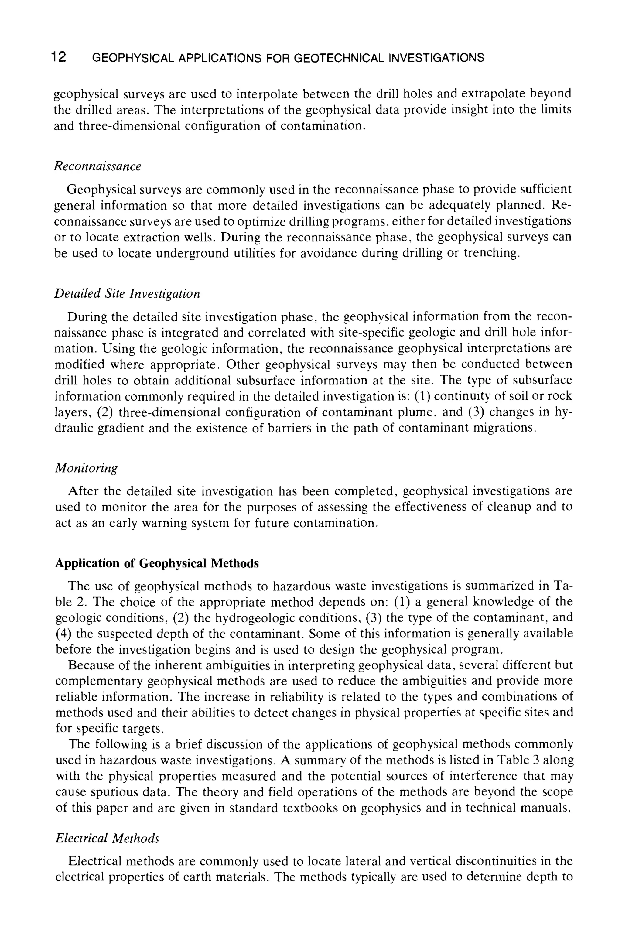
![18 GEOPHYSICALAPPLICATIONS FOR GEOTECHNICAL INVESTIGATIONS
and radar tomography, were conducted to obtain information on the physical properties
and distribution of the fracture zones. These methods were adequate to obtain information
about rock quality.
This paper describes the features of geotomography, presents results of the investigation,
and indicates the applicability of geotomography to rock investigations.
Features of Geotomography
Geotomography has attracted a great deal of attention as a method of investigating in
detail the distribution of underground physical properties [1]. Geotomography reconstructs
images of underground structures using a large data set. For this reason, geotomography
provides more information than surface geophysical survey methods. The three specific
advantages of geotomography over conventional surface surveys are: (1) the target area is
illuminated from several different angles, (2) the application of source transducers at points
in boreholes near the target allow for increased spatial resolution, and (3) the application
of sources in boreholes means that measurements are not degraded by propagation through
the shallow, extensively weathered zone.
Three kinds of geotomographic methods were used: (1) seismic tomography, (2) resistivity
tomography, and (3) radar tomography. The seismic wave velocity, the resistivity, or the
electromagnetic wave velocity are influenced by physical (rock) properties such as hardness,
condition of cracks, water content, or clay content. Because the response obtained by one
method may not be adequate to characterize all physical properties, it is effective to combine
different geotomographic methods to obtain a good image of the ground structure.
Characteristics of each geotomographic method are as follows.
Seismic Tornography
Seismic tomography reconstructs the seismic wave velocity distribution in the ground.
Seismic wave velocity varies according to rock type, degree of weathering, degree of meta-
morphism, number of cracks, and so forth. In this survey, the fracture zones are expected
to have lower seismic velocities than unfractured rock.
Resistivity Tomography
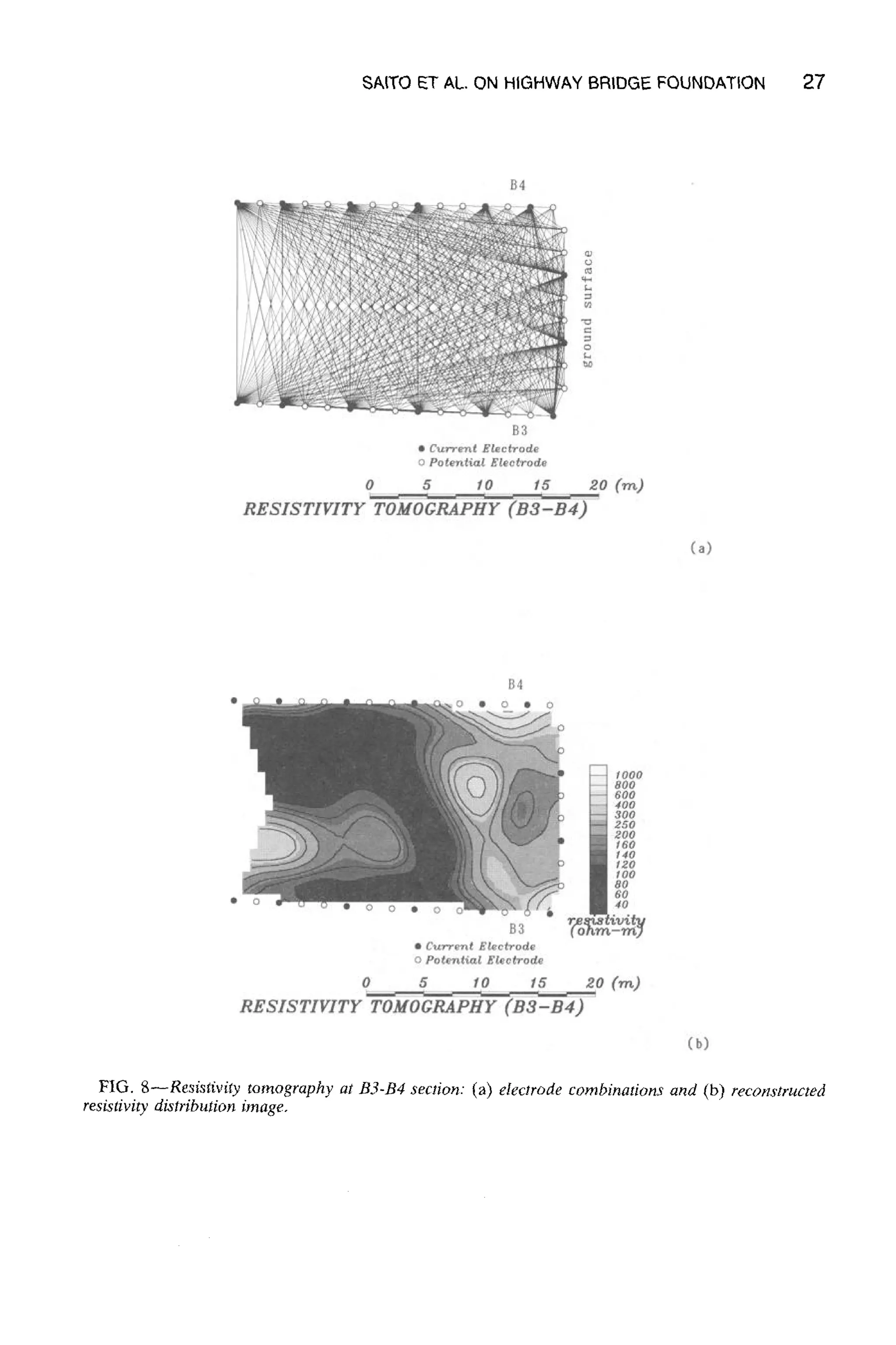
Resistivity tomography obtains the distribution of resistivity in the ground. Resistivity in
the ground changes according to rock type, mineral content, porosity, degree of saturation,
and the resistivity of water contained in the rock. In this survey, faults or fracture zones
are expected to have lower resistivity values than unfractured rock.
Radar Tomography
Radar tomography obtains the distribution of the propagation velocity of electromagnetic
waves in the ground. The propagation velocity of electromagnetic waves changes mainly
according to the water content of the rock. In this survey, the fracture zones are expected
to have lower velocities than unfractured rock.
Field Measurements and Results
Borehole Arrangernent
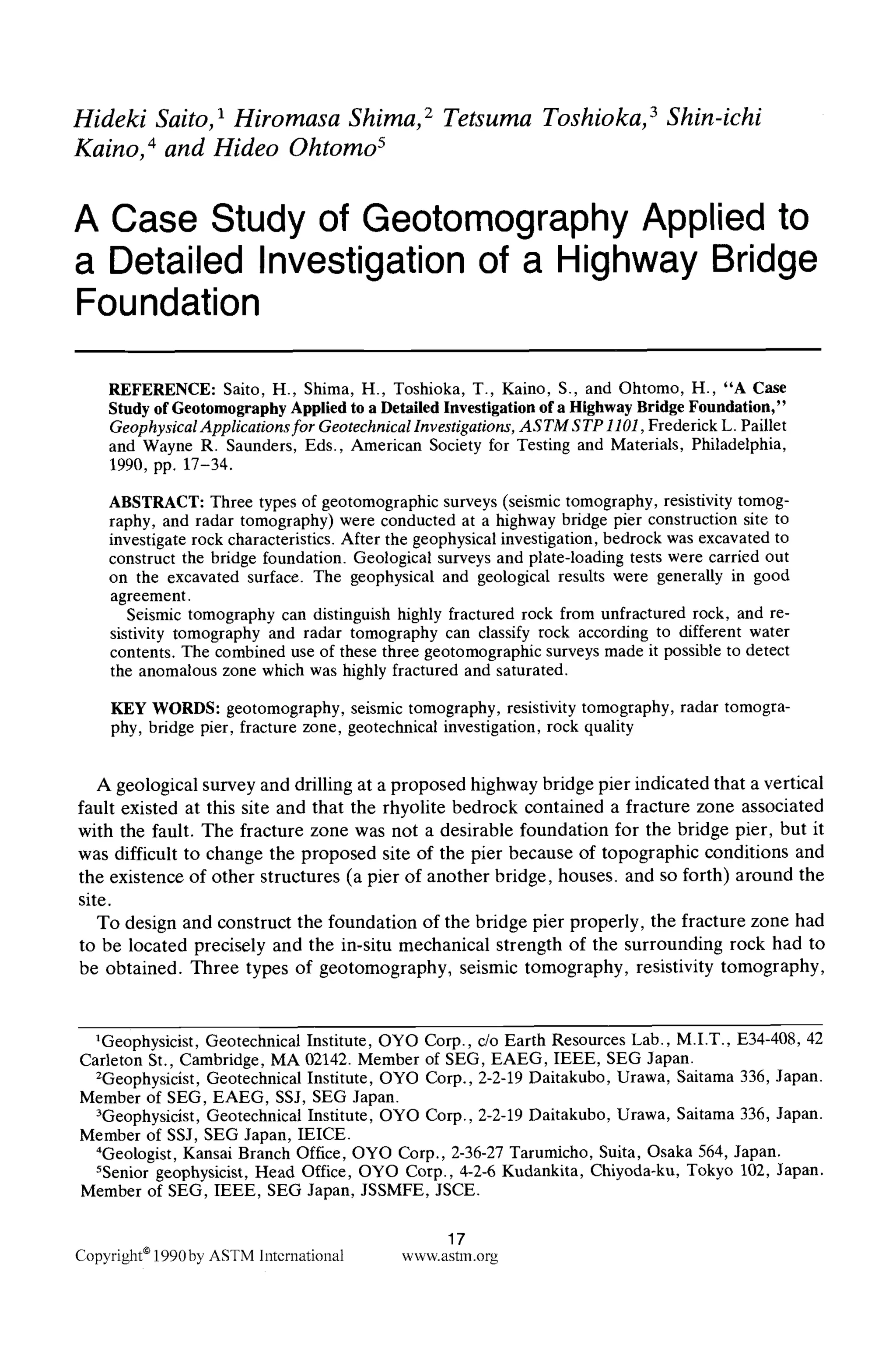
The previous geological survey indicated that the dip angle of the fracture zone was almost
vertical. When the predominant direction of the geological structure is nearly vertical,](https://image.slidesharecdn.com/geophysicalapplicationsforgeotechnicalinvestigations-151104153926-lva1-app6892/75/Geotechnical-Geophysics-21-2048.jpg)
![SAITO ET AL. ON HIGHWAY BRIDGEFOUNDATION 19
tomography using only vertical boreholes cannot provide a good reconstruction image [2].
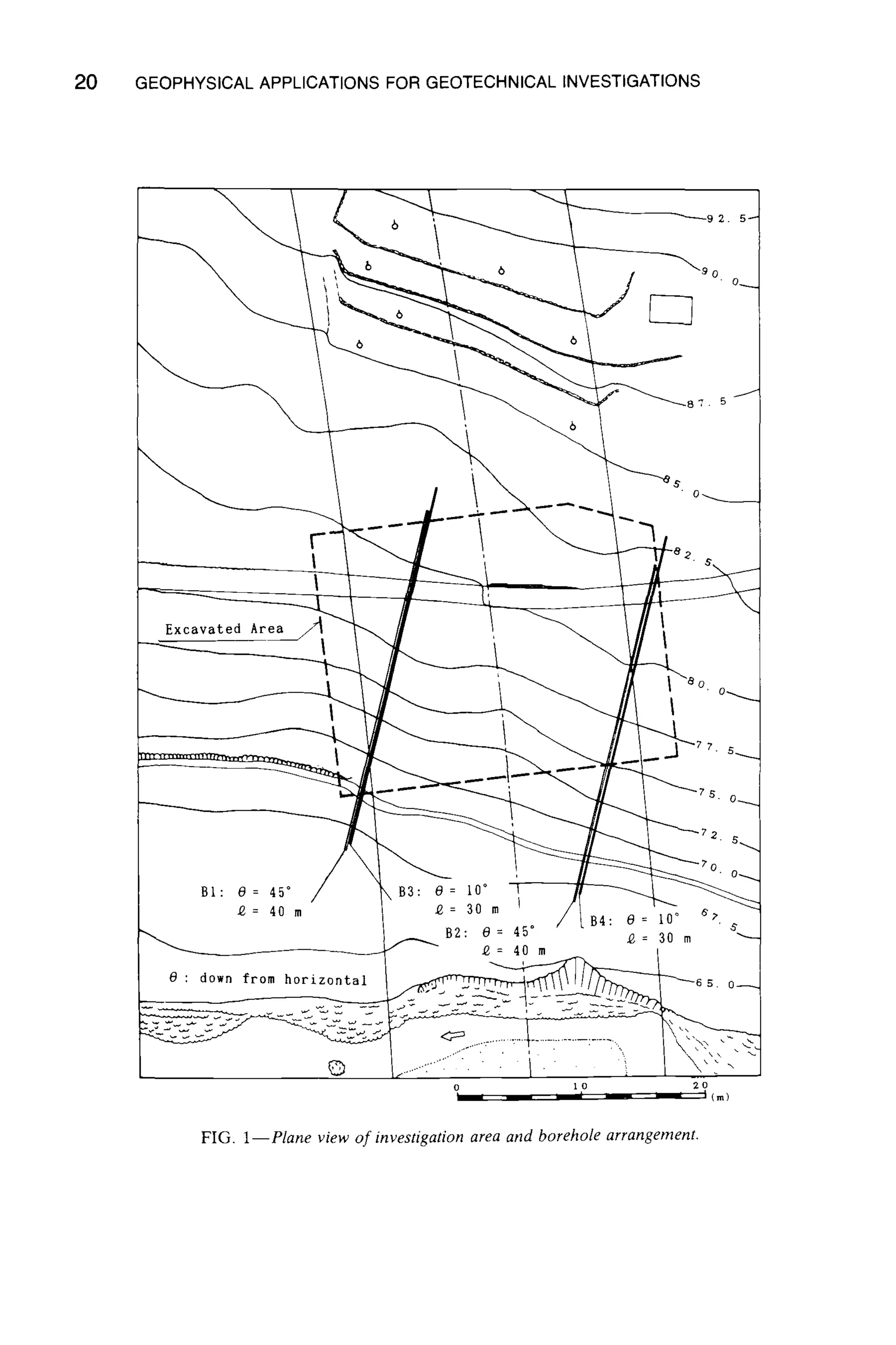
Therefore, four boreholes were drilled as shown in Figs. 1 and 2. Boreholes B1 and B2
were drilled at 45~ down from the horizontal and were 40 m long. Boreholes B3 and B4
were drilled at 10~ and were 30 m long.
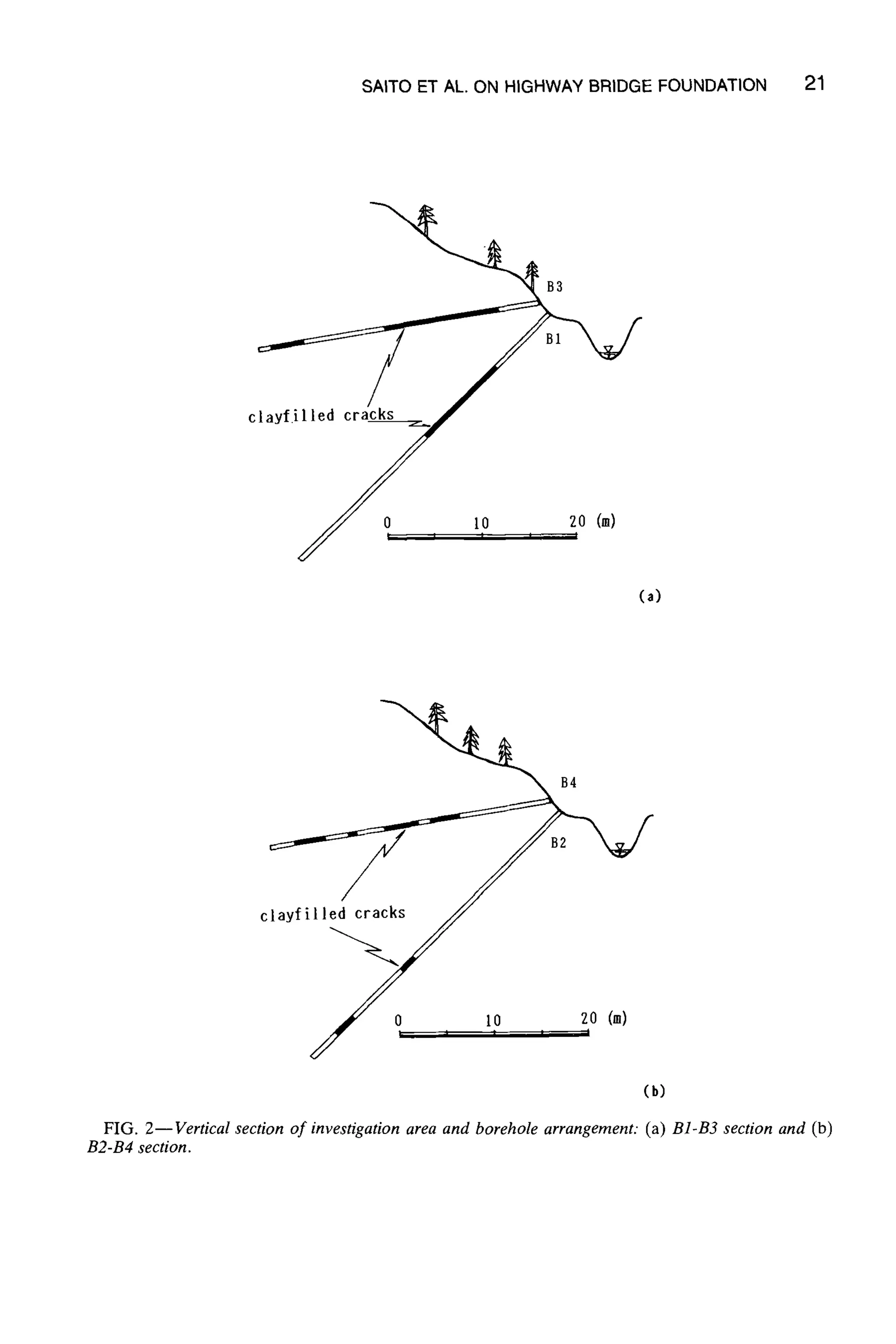
Seismic Tomography
The measurements for seismic tomography were conducted by surrounding the objective
section with source points and receiver points placed in boreholes and on the ground surface
between boreholes. Both source and receiver intervals were 2 m. About 50 g of dynamite
was used as the seismic source. Three sets of twelve-channel borehole geophones and eleven
geophones on the ground surface were used for measurements. A forty-eight-channel digital
data acquisition system (OYO's McSEIS 1600 System) was used.
The objective area was divided into a number of rectangular cells, and the velocity value
for each cell was obtained by an iterative method. In the iterative method, the velocity
(value) for each cell was corrected to minimize the root mean squares of residuals between
calculated and observed travel times. To prevent the divergence of the correction values,
the damped least squares technique was used [3]. The damping parameters were determined
by taking account of the number and directionality of seismic rays passing through each
cell [4].
The measurements were conducted at two vertical sections (B1-B3 and B2-B4), a 10~
section (B3-B4), and a 45~section (B1-B2). The results for the two vertical sections and the
10~ section are compared with the results of another tomographic techniques. Figures 3
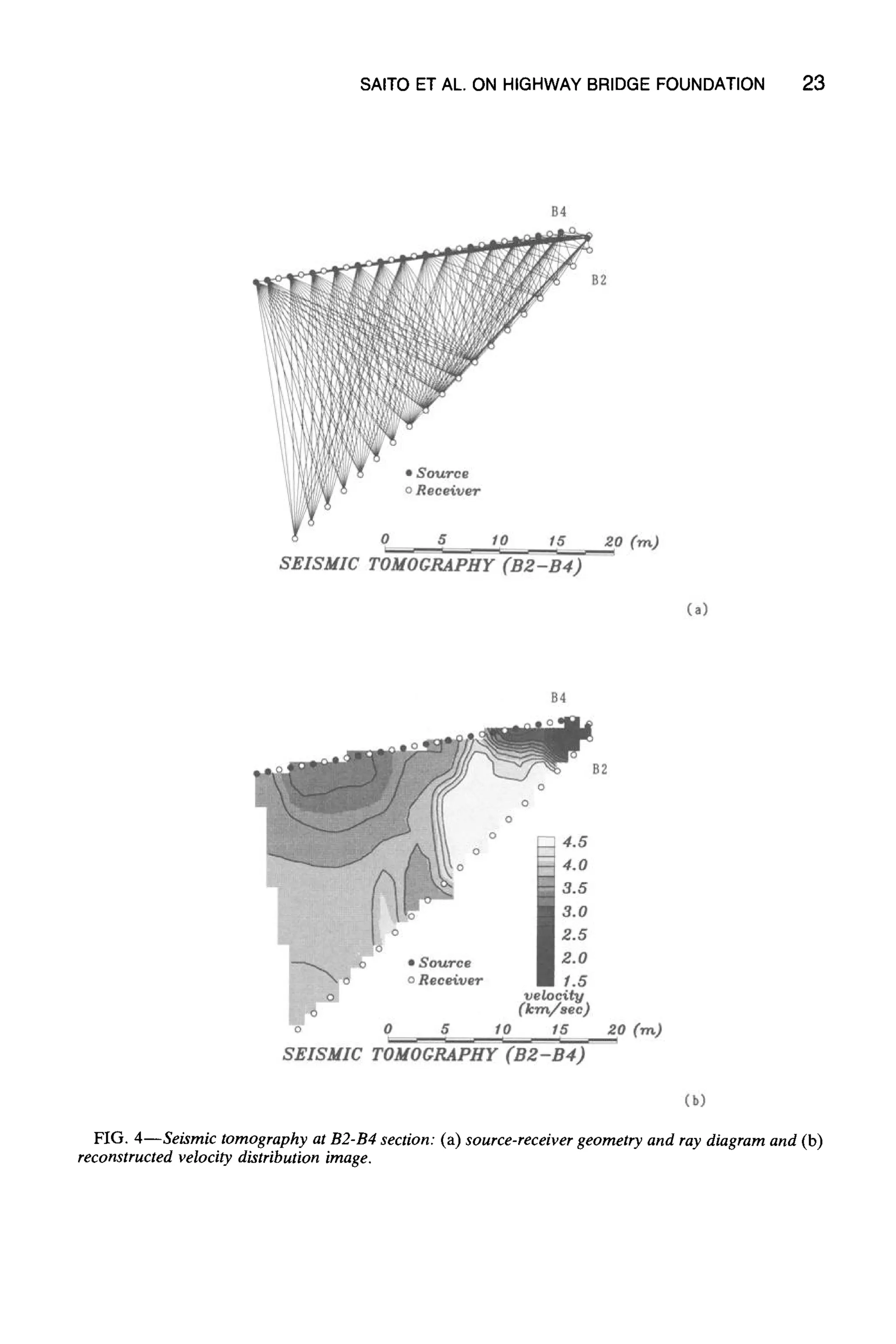
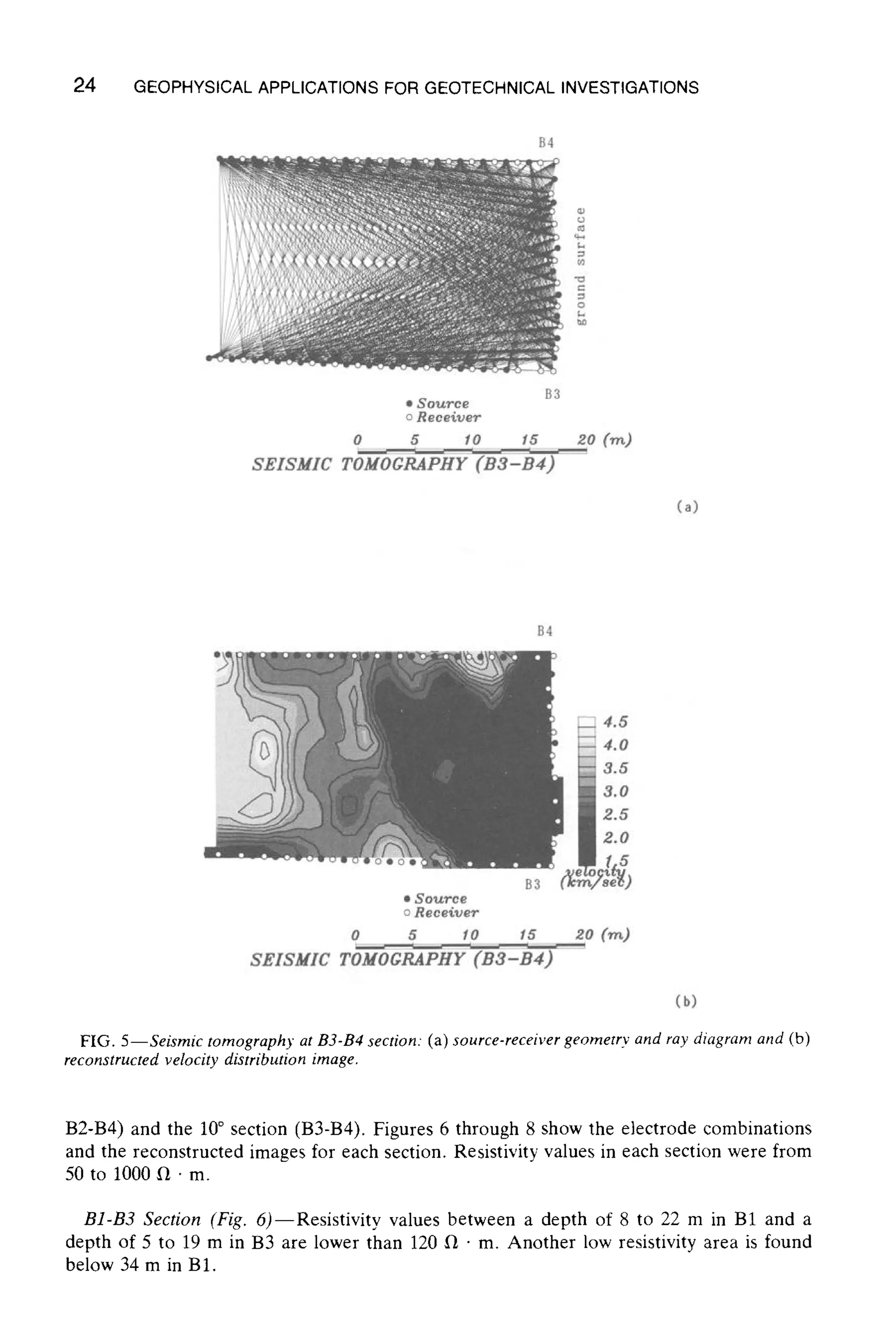
through 5 show source-receiver geometries, ray diagrams, and reconstructed velocity dis-
tribution images for each section.
B1-B3 Section (Fig. 3)--The P-wave velocity distribution of the B1-B3 section is shown
in Fig. 3b. Velocity values are indicated by shades of gray. Low velocity zones occur closer
to the surface-and between 8 to 19 m in Section B1 and 5 to 22 m in Section B3.
B2-B4 Section (Fig. 4)--Low velocity zones are found near the tops of the boreholes and
around the center of the area vertically. Between these low velocity zones, there is an
extremely high velocity zone.
B3-B4 Section (Fig. 5)--Nearly half of this section is a low velocity area with a velocity
of 2.5 km/s or lower.
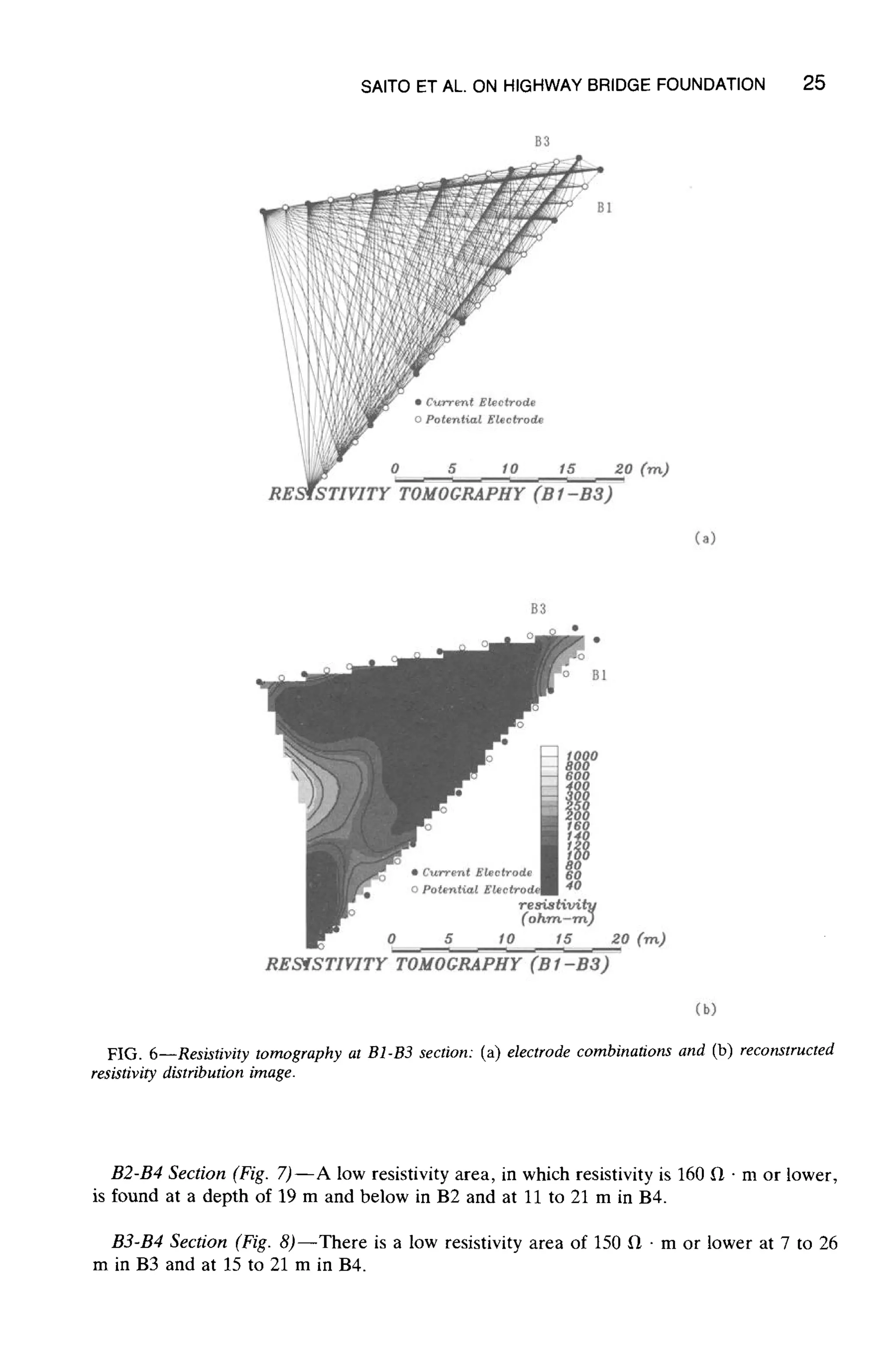
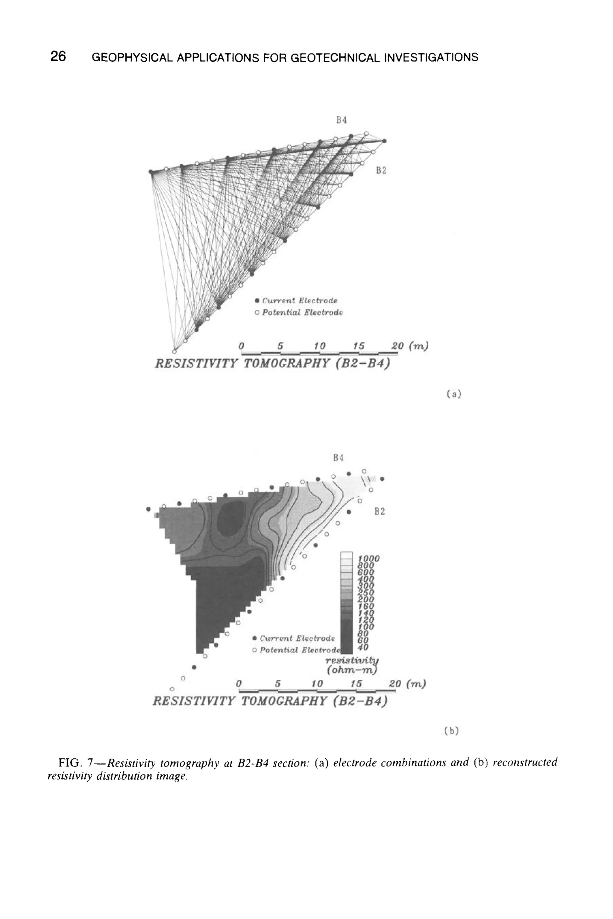
Resistivity Tomography
Resistivity tomography is a two-dimensional resistivity exploration method having higher
resolution than the conventional resistivity exploration method [5].
Electrodes were placed at 2-m intervals in the borehol.es and on the ground surface between
boreholes surrounding the objective area. Electric potential was measured by the pole-pole
array method using OYO's McOHM resistivity meter.
Analysis was conducted by a combination of the alpha centers method and the nonlinear
least squares method [5]. The electric potential at each potential electrode was theoretically
calculated by the alpha centers method. The resistivity distribution was corrected to minimize
the root mean squares of the residuals between calculated and observed electric potentials
by the nonlinear least squares method.
The objective sections for resistivity tomography were two vertical sections (B1-B3 and](https://image.slidesharecdn.com/geophysicalapplicationsforgeotechnicalinvestigations-151104153926-lva1-app6892/75/Geotechnical-Geophysics-22-2048.jpg)
![28 GEOPHYSICALAPPLICATIONS FOR GEOTECHNICAL INVESTIGATIONS
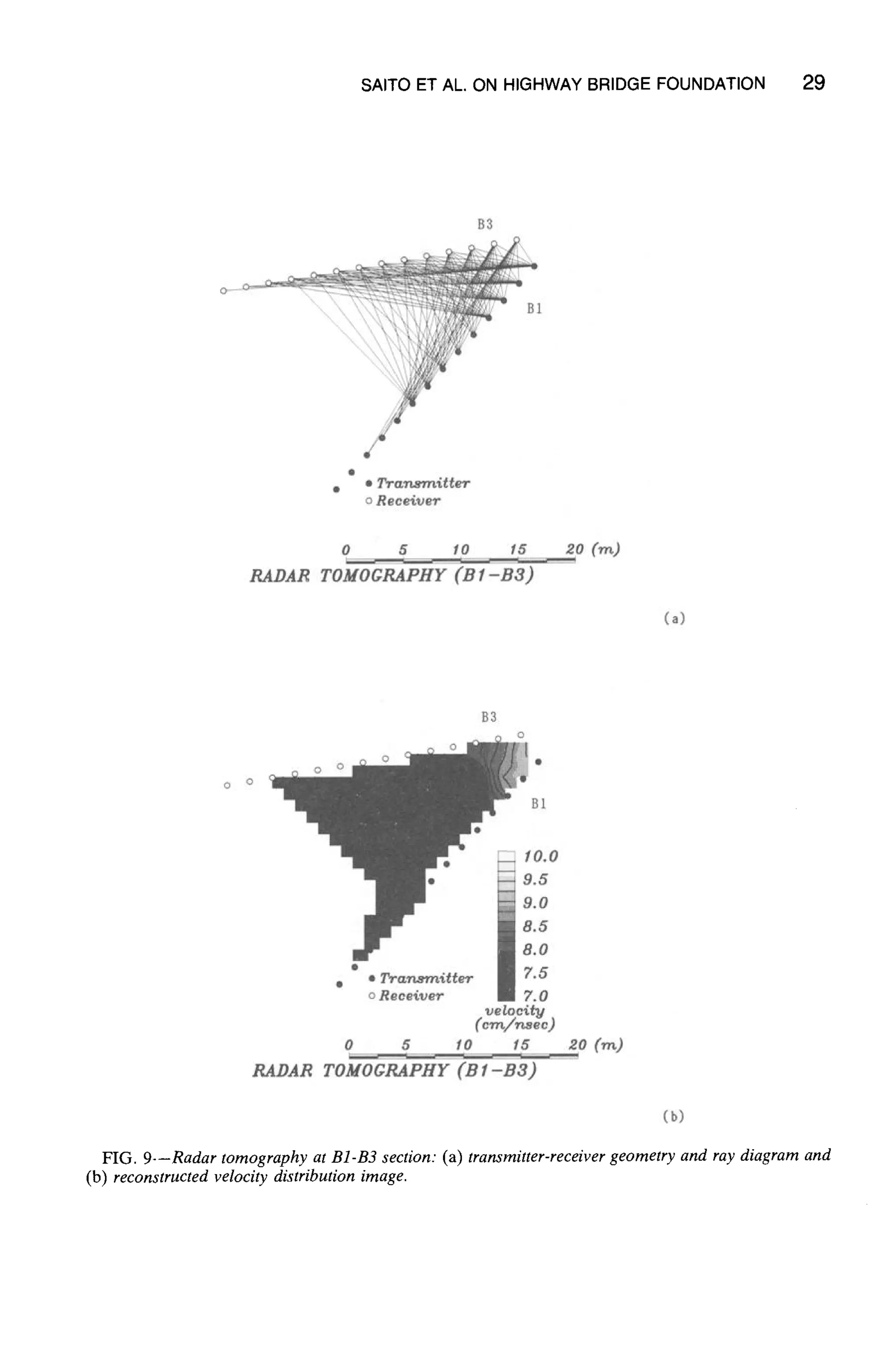
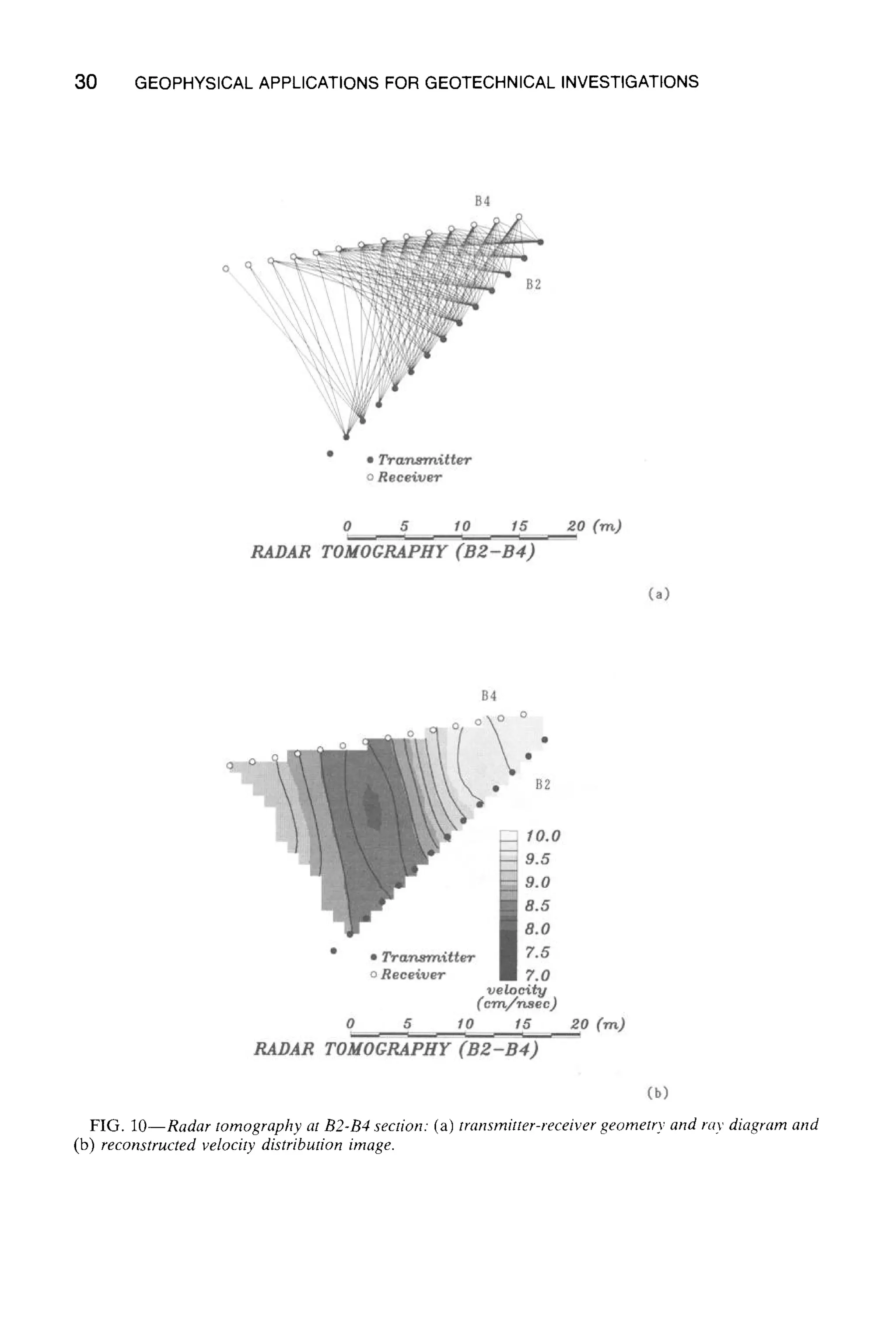
Radar Tomography
In radar tomography, electromagnetic pulse waves are transmitted from one antenna
located in a borehole to a receiving antenna in another borehole. Each antenna was moved
at 2-m intervals. The measurement system used was OYO's YL-R2 Georadar system. The
borehole antennas were especially constructed for experimental use. The center frequency
of the antennas was about 100 MHz and transmitted power was 50 W [6]. The same analysis
procedure as that used in seismic tomography was used in radar tomography.
Attenuation of electromagnetic waves at this site was so high that significant signals could
not be received in horizontal sections. Therefore. the measurements were conducted only
at two vertical sections. Figures 9 and 10 show the transmitting and receiving points, ray
diagrams, and the electromagnetic wave velocity distribution.
B1-B3 Section (Fig. 9)--Electromagnetic wave velocity is relatively lower than the velocity
values in the B2-B4 section. It is estimated, therefore, that water content in the bedrock at
the B1-B3 section is rather high. The area at the depth of 7 m or below has low velocity
and is estimated to be a fracture zone having high water content.
B2-B4 Section (Fig. lO)--The zone, below 16 m in B2 and from 13 to 21 m in B4, is a
low velocity zone that continues vertically and is considered to be bedrock having high water
content.
Consideration
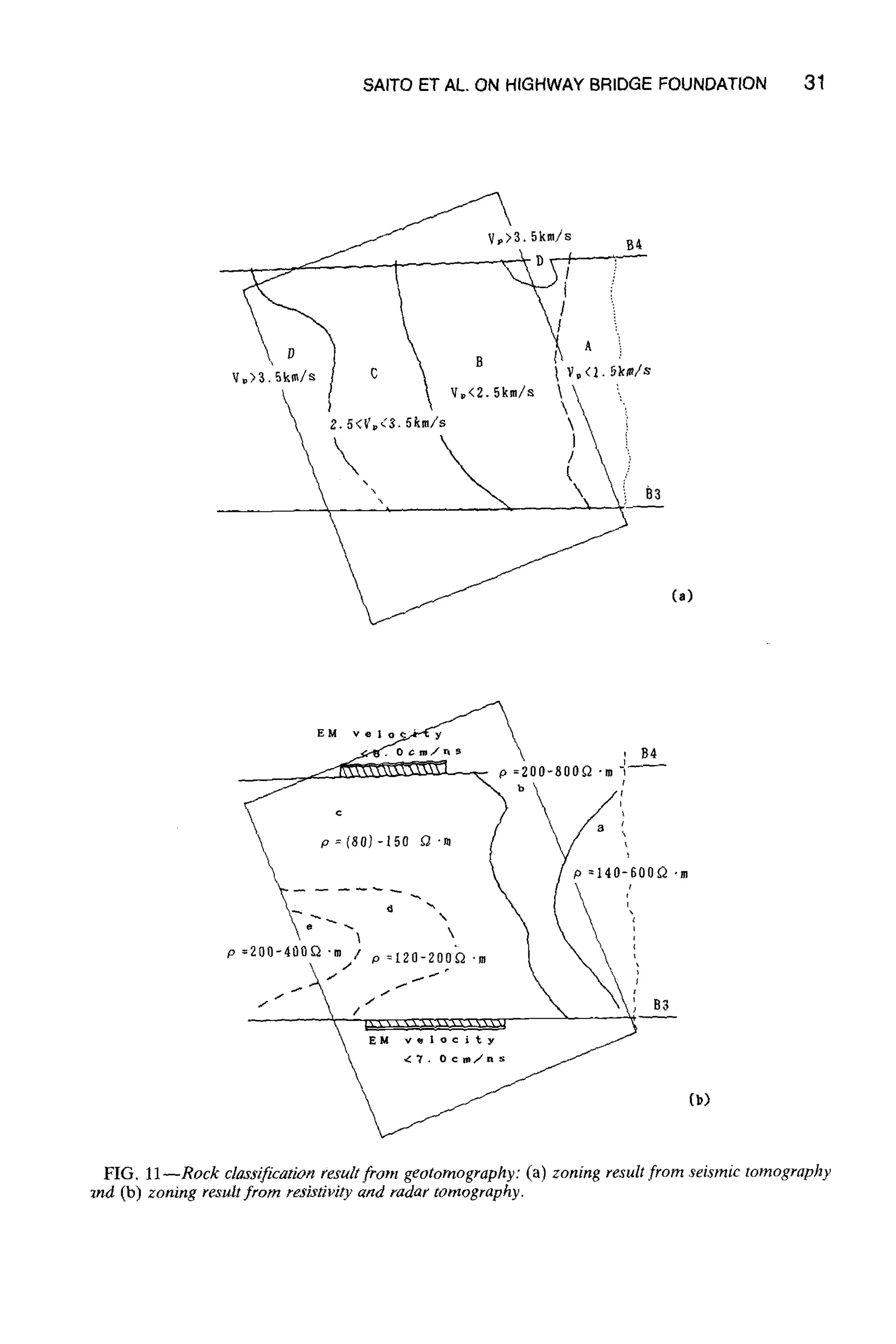
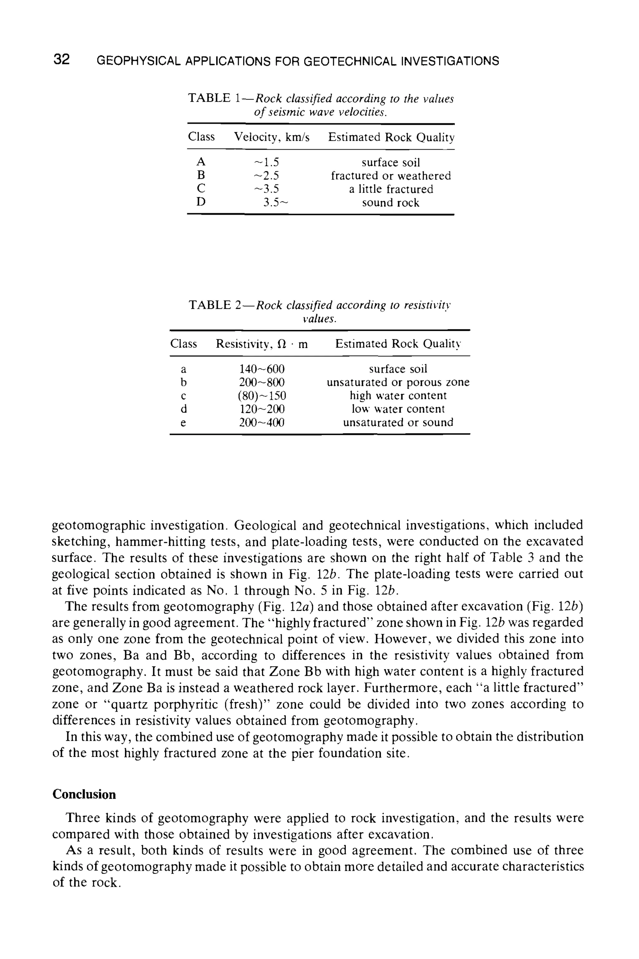
Based on the results of geotomography, we conducted an analysis of rock quality in the
B3-B4 section. We tried to classify the rock according to the values of seismic wave velocities
as shown in Fig. 11a and Table 1.
Since the seismic wave velocity is closely related to the mechanical strength of rock, it
can be said that this figure shows the distribution of mechanical properties of rock.
In this investigation site, the relative variation of resistivity depends mainly on water
content and the quantity of clay that was formed through alteration or fracturing. We tried
to classify the rock according to resistivity values, as shown in Fig. llb and Table 2.
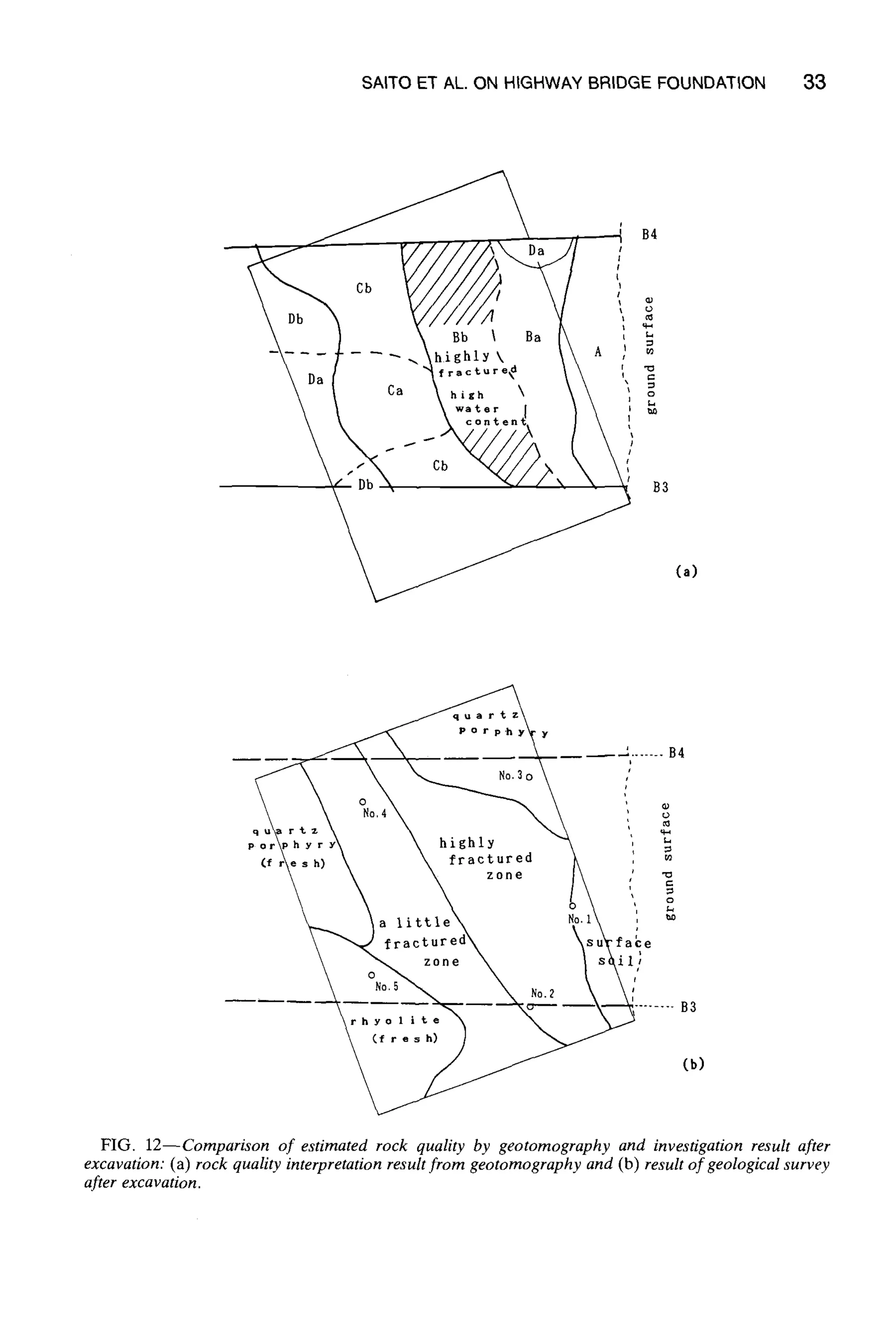
Next, we tried to analyze the rock quality by using the results of seismic tomography
along with the results of resistivity tomography. The final analysis result of tomographic
investigations is shown in Fig. 12a.
Zone A was considered to be the surface soil layer having low seismic wave velocity and
high resistivity. Zones B, C, and D were each divided into two areas of high resistivity or
low resistivity. Zone Ba was considered to be weathered but unsaturated rock distributed
near the surface which had low seismic wave velocity and relatively high resistivity. Zone
Bb was considered to be a highly fractured zone of high water content which had low seismic
wave velocity and low resistivity. Both Zones Ca and Cb were considered to be a little
fractured, but the water content differed from each other. Zone Ca was considered to have
rather low water content which had rather low seismic wave velocity and a little low resistivity.
Zone Cb was considered to have high water content which had rather low seismic wave
velocity and low resistivity. Both Zones Da and Db were relatively fresh and sound rock,
however, Zone Db had rather high water content.
Consequently, it can be said that Zones Bb, Ca, and Cb correspond to fracture zones.
In particular, Zone Bb is considered to correspond to the most highly fractured zone having
high water content. The results mentioned above are shown in the left half of Table 3.
Excavation for the construction of the bridge pier foundation was carried out after the](https://image.slidesharecdn.com/geophysicalapplicationsforgeotechnicalinvestigations-151104153926-lva1-app6892/75/Geotechnical-Geophysics-31-2048.jpg)
![34 GEOPHYSICAL APPLICATIONS FOR GEOTECHNICAL INVESTIGATIONS
TABLE 3--Results from geotomography and investigationsafter excavation
Results from Geotomography
Results from Investigations after
Excavation
Seismic Deformation
Velocity, Resistivity, Estimated Constant,
Class km/s ~ 9m Quality Quality kgf/cmz
A -1.5 140-600 surface soil surface soil
weathered
Ba 200-800 (unsaturated)
-2.5 highly fractured
highly fractured
Bb 80-150 and high
water content
a little fractured
and rather
Ca 120~200
low water
content
-3.5 a little fractured
a little fractured
Cb 80-150 and high
water content
290
(No. 1 point)
160
(No. 2 point)
650
(No. 4 point)
quartz porphyry 1900
Da 200-400 sound or fresh (fresh) (No. 3 point)
3.5-
sound and rhyolite (fresh)
Db 80-150 rather high 840
water content (No. 5 point)
In the future, we intend to apply geotomography to many other sites having various
geological conditions and to conduct further studies on the applicability of geotomography
for civil engineering purposes.
References
[1] Sassa, K., "Suggested Methods for Seismic Testing Within and Between Boreholes,'" International
Journal of Rock Mechanic Sciences and Geomechanics Abstracts, Vol. 25, No. 6, 1988, pp. 447-
472.
[2] Sakayama, T., Ohtomo, H., Saito, H., and Shima. H., "Applicability and Some Problems Of
Geophysical Tomography Techniques in Estimation of Underground Structure and Physical Prop-
erties of Rock," presented at the 2nd International Symposium on Field Measurements in Geo-
mechanics, Kobe, Japan, April 1987.
[3] Aki, K. and Lee, W. H. K., "Determination of Three-Dimensional Velocity Anomalies Under a
Seismic Array Using First P Arrival Times from Local Earthquakes," Journal of Geophysical
Research, Vol. 81, 1976, pp. 4381-4399.
[4] Saito, H. and Ohtomo, H., "Seismic Ray Tomography Using the Method of Damped Least Squares,"
Exploration Geophysics. Vol. 19, Nos. 1/2, 1988. pp. 348-351.
[5} Shima, H. and Sakayama, T., "Resistivity Tomography: An Approach to 2-D Resistivity Inverse
Problems," presented at the 57th SEG Annual International Meeting, New Orleans, Oct. 1987.
[6] Toshioka, T. and Sakayama, T., "Preliminary Description of Borehole Radar and First Results,"
presented at the 76th SEGJ Conference, Tokyo, Japan, April 1987.](https://image.slidesharecdn.com/geophysicalapplicationsforgeotechnicalinvestigations-151104153926-lva1-app6892/75/Geotechnical-Geophysics-37-2048.jpg)

![Robert E. Crowder, 1 Larry A. Irons, 2 and Elliot N. Yearsley ~
Economic Considerations of Borehole
Geophysics for Hazardous Waste Projects
REFERENCE: Crowder, R. E., Irons, L. A., and Yearsley, E. N., "Economic Considerations
of Borehole Geophysics for Hazardous Waste Projects," Geophysical Applications for Geo-
technical Investigations, ASTM STP 1101, Frederick L. Paillet and Wayne R. Saunders, Eds.,
American Society for Testing and Materials, Philadelphia, 1990, pp. 37-46.
ABSTRACT: In environmental or hazardous waste investigations, simple homogenous sub-
surface geologic conditions have historically been assumed. In reality, heterogeneous condi-
tions predominate. The costs of remediation and the consequences of incorrect remediation
are increasing rapidly. These investigations often require the collection of extensive amounts
of data to evaluate the problems sufficientlyto recommend and execute appropriate remedial
action.
Borehole geophysics can be used to obtain valuable data including information on geologic
conditions and in-situ physical parameters in drill holes. The amount and benefit of this
information is determined by the logging suite, borehole conditions, geologic parameters,
interpreter experience, and application of current technology.
Typical costs for drilling and geophysical logging associated with different types of environ-
mental investigations vary considerably. These costs are a function of the types and quantity
of the desired data, whether the geophysical logging and analysis will be performed in-house
or by an outside consultant, and the operational field environment.
Five case histories demonstrate the application of borehole geophysics to hazardous waste
investigations and provide qualitative evidence as to its cost-effectiveness. The primary con-
clusionsindicated by these case histories are that: (1) geophysical logs assist in well construction
efforts; (2) borehole geophysical logs provide in-situphysical measurements not available from
other methods; and (3) costs associated with borehole loggingcan be justified by consideration
of the total cost of drilling, completion, and monitoring and the implications of inadequate
understanding of the subsurface in a remediation program.
KEY WORDS: borehole geophysics, monitor well, cost, hazardous waste site investigations
In environmental investigations for ground-water contamination problems, simple, ho-
mogenous subsurface geologic conditions have historically been assumed. These site char-
acterizations are proving to be more difficult than originally anticipated, and a number of
prior investigations appear to be flawed. A U.S. Environmental Protection Agency (EPA)
study [1] of 22 Resource Conservation and Recovery Act (RCRA) sites showed problems
including:
(1) incorrect screening in 50% of the monitoring wells,
(2) incorrect placement of 30% of the wells, and
(3) on 10% of the sites, Wells were placed before determining the direction of ground-
water flow.
1President and geological engineer, respectively, Colog, Inc., 10198th St., Golden, CO 80401.
2Senior associate geophysicist, Ebasco/Envirosphere Co., 143 Union Blvd,, Suite 1010, Lakewood,
CO 80228.
37
Copyright91990by ASTM International www.astm.org](https://image.slidesharecdn.com/geophysicalapplicationsforgeotechnicalinvestigations-151104153926-lva1-app6892/75/Geotechnical-Geophysics-39-2048.jpg)
![38 GEOPHYSICALAPPLICATIONS FOR GEOTECHNICAL INVESTIGATIONS
The geologic conditions encountered on most of these sites are complex and often require
collecting extensive amounts of data to evaluate the problems sufficiently to recommend
and execute the appropriate remedial action. The costs of remediation and the consequences
of incorrect remediation are increasing rapidly [2]. Each project is unique in certain respects
because the particular environment, potential contaminant, and goals will all be somewhat
different.
The purpose of this paper is to convey experience and information regarding the economic
considerations involved in obtaining subsurface data relevant to hazardous waste investi-
gations. Discussions contained herein outline the benefits of the application of borehole
geophysics to the problem of subsurface interpretation. These discussions provide guidelines
and considerations for geophysical logging operations and costs and review historical prac-
tices and costs of drilling, coring, testing, and geochemical analyses.
The common thread in these topics is their application toward the investigation and
characterization of hazardous (or potentially hazardous) waste sites. The relative cost-
effectiveness of borehole geophysics in these efforts is addressed. The thesis of this paper
is that borehole geophysics provides a cost-effective means for the subsurface investigations
of these sites. Furthermore, that the existential measurements provided by borehole geo-
physics complement core data, support surface geophysics, and offer geologic and hydro-
geologic information not otherwise available.
Borehole Geophysical Logging Considerations and Benefits
There is no uniform logging suite applicable to every project, and no unambiguous rules
for log interpretation exist. Most log analyses in ground-water investigations are based upon
techniques developed by the petroleum industry. These techniques may not be directly
applicable when applied to shallow ground-water investigations, and less experience and
scientific literature is available in this area. Many ground-water engineers and geologists
have no formal training in the use of borehole geophysics, whereas their counterparts in
the petroleum industry are well trained in the use of these logs.
Furthermore, logging tools developed for the petroleum industry are inadequate for the
shallow depth and small-diameter applications encountered in most environmental inves-
tigations. Many monitoring wells are drilled and completed with hollow-stem auger tech-
niques in the vadose zone. Logging in the vadose or unsaturated zone is feasible and provides
valuable information not available elsewhere, but disturbances to the formation from drilling
in this zone may produce large changes on the logs. Quantitative analysis usually requires
information from several types of logs. Sometimes the drill holes are not stable enough for
open-hole logging or to allow more than one open hole pass by a geophysical probe, and
the selection of probes for the initial pass requires careful consideration. Radioactive sources
required for some measurements are regulated, and the use of these sources may not be
feasible to use on some projects.
Many environmental projects are located in areas distant with respect to the historical
petroleum and mineral industry service companies, often requiring expensive mobilization.
Environmental projects frequently have a low production rate for drilling.new wells, both
in number and depth. The time lapse between wells may be several days. These factors
increase the logging costs. Health and safety training requirements can be a major burden
for many of the smaller slimhole logging contractors and may prevent them from entering
the environmental market.
Historically, only a few simple logs have been used in nonpetroleum applications. Many
people expect slimhole nonpetroleum logs for environmental applications to be inexpensive](https://image.slidesharecdn.com/geophysicalapplicationsforgeotechnicalinvestigations-151104153926-lva1-app6892/75/Geotechnical-Geophysics-40-2048.jpg)
![CROWDER ET AL. ON BOREHOLE GEOPHYSICS
TABLE 1--Direct benefits of borehole geophysics.
39
Broad Category Specific Aspects
Well construction
Physical properties
Stratigraphic
correlation
depth and identification of lithologicbeds, borehole size and volume,
water table
porosity, density, resistivity, temperature, fluid flow, water quality,
fracture identification, rock strength parameters
continuity of aquifers and confining beds based on cross-hole
correlation, facies changes
and accordingly do not budget for the necessary logs and interpretation. Many firms do not
have staff expertise to use much of the advanced geophysical information. For example,
knowledge may be limited to recognition of apparent sand-shale zones for screen selection
and may not include proper interpretation of the remaining data. The economics of running
a complex suite that cannot be properly used would appear questionable.
In spite of the above perceptions and hindrances to slimhole logging, borehole geophysics
has important benefits in hazardous waste investigations when interpreted properly [3].
These benefits can be classified as direct and indirect [4,5], as shown in Tables 1 and 2.
Borehole GeophysicalLogging Costs
Traditional logging costs were based upon a low service charge (base time rate), a footage
charge (based upon the types of probes and total project footage logged), and miscellaneous
expenses for such items as per diem and standby. Costs per foot were kept low by logging
high footages in many wells. Typically, the drill rig was not incurring standby charges on
energy/mineral exploration projects and the standby charges for the petroleum applications
were generally well understood by everyone involved with those projects.
The primary cost factor for most environmental logging programs is personnel and equip-
ment time. This time factor includes mobilization/demobilization to and from the project
area, standby waiting for a well to be finished, pre- and post-log calibration, data acquisition,
data processing, interpretation, and decontamination of personnel and equipment. For the
typical shallow wells encountered on most environmental investigations, actual data acqui-
sition time is the least significant aspect. Footage charges are difficult to compare to the
classical slimhole logging industry and tend to be a minor element in the overall cost. The
number and type of logs affect the overall costs in that it takes as long or longer to pre-
and post-calibrate, setup, and decontaminate on a shallow well as it does on a deep well.
However, on many projects, the cost to run one or several extra logs may be insignificant
TABLE 2--Indirect benefits of borehole geophysics.
1. Objective, repeatable data collected over a continuous vertical interval.
2. Digital data is conveniently stored, processed, and transmitted.
3. Log results are available at well site or shortly thereafter.
4. Borehole geophysical data is synergistic with core data, surface geophysics, and other
borehole geophysical data.
5. Borehole logs can be standardized to facilitate correlation between different phases of an
investigation by different firms.](https://image.slidesharecdn.com/geophysicalapplicationsforgeotechnicalinvestigations-151104153926-lva1-app6892/75/Geotechnical-Geophysics-41-2048.jpg)
![46 GEOPHYSICALAPPLICATIONS FOR GEOTECHNICAL INVESTIGATIONS
hole geophysics is a tool that has been underused on many of these projects: however, it
can be cost-effective in site investigation and also in long-term monitoring.
Primary reasons for the lack of use of borehole geophysics include a lack of understanding
of the methods, the availability of the services, the availability of log interpreters/analysts,
and a lack of understanding of the goals of the projects. As these goals become better
defined, the value of more objective log data increases. Education and experience are starting
to overcome some of this lack of understanding, and regulations are now stipulating minimal
geophysical logs on many projects. A better understanding of the limitations of the log data,
especially during acquisition, also aids in evaluating the information effectively.
Acknowledgments
The authors of this paper wish to thank Mr. Larry Dearborn with CE Environmental,
Ebasco Services, Inc., and the other engineering companies contacted for the sharing of
cost information used in this paper.
References
[1] Wheatcraft, S. W.. Taylor, K. C., Hess, J. W.. and Morris, T. M., 'Borehole Sensing Methods
for Ground-Water Investigations at Hazardous Waste Sites." Water Resources Center, Desert
Research Institute, University of Nevada System. Cooperative Agreement CR 810t)52 for Envi-
ronmental Monitoring Systems Laboratory, Office of Research and Development. U.S. EPA, Las
Vegas, NV 89114, Dec. 1986. Reproduced bv U.S. Department of Commerce. National Technical
Information Service, Springfield, VA 22161.
[2] Crowder, R. E. and Irons, L., "Economic Considerations of Borehole Geophysics for Engineering
and EnvironmentalProjects," in Proceedings of the Symposium on the Application of Geophysics
to Engineeringand Environmental Problems. Colorado School of Mines, Golden, CO. 1989.
[3] Crowder, R. E., "Cost Effectiveness of Drill Hole Geophysical Logging For Coal Exploration,"
paper presented at the Third InternationalCoal Exploration Symposium,Calgary, Alberta, Canada,
1981.
[4] Keys, S., "Borehole GeophysicsApplied to Ground-WaterInvestigations,'"U.S. Geological Survey,
Open-File Report 87-539, Dec. 1988.
[5] Stegner, R. and Becker, A., "Borehole Geophysical Methodology: Analysis and Comparison of
New TechnologiesFor GroundWater Investigation," in Proceedingsof the Second National Outdoor
Action Conference and Aquifer Restoration, Ground Water Monitoring and Geophysical Methods,
Vol. II, 1988.](https://image.slidesharecdn.com/geophysicalapplicationsforgeotechnicalinvestigations-151104153926-lva1-app6892/75/Geotechnical-Geophysics-48-2048.jpg)
![Donald G. Jorgensen I
Estimating Water Quality from Geophysical
Logs
REFERENCE: Jorgensen, D. G., "Estimating Water Quality from Geophysical Logs," Geo-
physicalApplicationsfor GeotechnicalInvestigations,ASTM STP 1101, Frederick L. Paillet
and Wayne R. Saunders, Eds., American Society for Testing and Materials, Philadelphia,
1990, pp. 47-64.
ABSTRACT: Borehole-geophysical logs can be used to obtain information on water quality
and water chemistry: Water quality characteristics that normally are measured directly in water-
filled holes or wells include chloride, dissolved oxygen, pH, temperature, and conductivity.
In-situ ground water may exist at some distance adjacent to the borehole, and estimates of
water quality or water chemistry can be made by measuring the resistivity or specific electrical
conductivity of the water in pore spaces. Most geophysical logs, however, are made in test
holes filled with drilling fluid. In this environment, logs enabling estimates of water resistivity
(Rw) are useful. Relations among Rw and dissolved solids, sodium chloride solutions, and
temperature are well established for saline waters; for freshwater, however, the activities of
other dissolved ions also need to be considered. The spontaneous potential (SP) is a function
of activity of the mud filtrate and water resistivity and, thus, can be used to estimate Rw.
Two methods of estimating Rw are useful: the spontaneous potential (SP) method, which
uses data from a spontaneous potential log and a resistivity log, and the cross-plot method,
which uses log-derived porosity and resistivity-log data. The application of SP logs depends
upon the water quality contrast between the water in the pores (Rw)and the mud filtrate on
the borehole wall. Both methods estimate Rw to about a half order of magnitude. However,
the accuracy of both methods can be greatly improved if additional data, such as a chemical
analysis, can be correlated to a log.
KEY WORDS: geophysical logging, spontaneous potential, resistivity, ground-water quality
The chemical constituents of water affect the responses of nearly all borehole-geophysical
logs. Thus, borehole-geophysical logs normally contain information on water quality that
can be extracted by using various methods of analysis.
This paper describes how borehole-geophysical logs can be used to estimate water chem-
istry; however, the scope of this paper excludes a description of logging tools, except in a
very general way, and the physics that affect the responses measured by the wireline tool.
Detailed information of various geophysical logs can be obtained from textbooks such as
Log Analysis of Subsurface Geology [1] and WellLogging of Physical Properties [2], industry
manuals such as Log Interpretation Principles/Applications [3] and Log Interpretation
Fundamentals [4], or special texts such as Borehole Geophysics Applied to Ground-Water
Investigations [5]. In general, the problems of quantitatively evaluating clay content or
"shaleyness" from borehole-geophysical logs is beyond the scope of this paper. However,
1Hydrologist, U.S. Geological Survey, P.O. Box 25046, Mail Stop 421, Denver Federal Center,
Denver, CO 80225-0046.
2R. Leonard, written communication, U.S. Geological Survey, 1984.
47
Copyright9 1990by ASTM International www.astm.org](https://image.slidesharecdn.com/geophysicalapplicationsforgeotechnicalinvestigations-151104153926-lva1-app6892/75/Geotechnical-Geophysics-49-2048.jpg)
![48 GEOPHYSICALAPPLICATIONSFOR GEOTECHNICALINVESTIGATIONS
qualitative evaluation of clay content generally can be made from the response recorded by
a gamma-ray log.
The techniques presented in this paper greatly rely on relations among temperature,
density, and resistivity to water chemistry properties, such as concentrations of dissolved
solids, sodium chloride, and chloride. These relations are given in the appendices. Material
presented herein relies heavily on the material published in the U.S. Geological Survey
Water Supply Paper 2321, "Some Uses of Geophysical Logs to Estimate Porosity, Water
Resistivity, and Intrinsic Permeability" [6].
Direct measurements of formation water quality or water chemistry can be made only in
water wells, provided the water in the well is the same as that in the adjacent formation.
Thus, a direct-measuring borehole-geophysical probe can measure the variation with the
depth of different water quality or water chemistry properties. However, because of slight
differences in head that exist in any transient ground-water flow system, the well bore causes
a "short circuit" and water flows into the borehole. This flow complicates the interpretation
of direct-measuring geophysical logs made by probes used in the downhole measurements
of chemistry and water quality in a particular geohydrologic zone penetrated by the borehole.
Water chemistry information can be obtained indirectly from borehole-geophysical logs
run in holes filled with drilling fluids. Under these conditions, unaltered or uncontaminated
aquifer water typically is found adjacent to the annulus of the borehole. In addition to
drilling fluid in the borehole, it is likely there is a mud cake or mud filter formed on the
borehole wall. Drilling fluid typically is forced through the mud filter and invades the adjacent
formations for various distances; that is, mud filtrate invades the formation, Thus, water
chemistry cannot be measured directly. To determine water chemistry in the formation (or
aquifer) by using borehole-geophysical logs, it is necessary to differentiate among the effects
of the drilling fluid, mud filter, invading mud filtrate, and the effects of the rock material
that contains the ground water.
Direct Measurement Methods
A small number of borehole probes (tools) directly measure certain water chemistry
properties. For example, special probes have been developed that measure chloride and
dissolved oxygen. Other special probes directly measure water quality properties such as
pH, temperature, and conductivity.
Other borehole tools include water-sampling mechanisms (thief samplers); although not
strictly borehole geophysical probes, these devices commonly are associated with geophysical
logging and often use the same wireline as is used to support geophysical probes. Unfor-
tunately, direct-measuring chemistry probes are few, and, accordingly, indirect methods,
such as correlation of resistivity to water chemistry, are used as surrogates.
Indirect Measurement Methods
Numerous data have been collected that relate resistivity of water to the concentrations
of dissolved solids, sodium, or chloride. In general, these relations are appropriate for saline
water (herein, water with dissolved solids concentrations exceeding 700 mg/L is considered
slightly saline and water exceeding 2000 mg/L is considered saline). Nearly all borehole-
geophysical logging interpretive techniques developed for the oil industry are based on
sodium chloride (NaC1) saline water. Numerous interpretive techniques are available from
the oil industry. Many of these techniques use a resistivity measurement of water based on
a saline, NaC1 water.](https://image.slidesharecdn.com/geophysicalapplicationsforgeotechnicalinvestigations-151104153926-lva1-app6892/75/Geotechnical-Geophysics-50-2048.jpg)
![JORGENSEN ON ESTIMATINGWATER QUALITY 49
Resistivity and Water Chemistry
Water resistivity is a measure of the resistance of a unit volume of water to electric flow
and is related to water chemistry and temperature. Water that contains a small concentration
of dissolved material has a large electrical resistance. Water that contains a large concen-
tration of dissolved solids has a smaller resistance. Quantitative techniques are available for
identifying water resistivity, which is a characteristic that can be related to the chemistry of
the water. The relation of dissolved solids and common chemical constituents to water
resistivity commonly is known (see Appendixes A and B) or can be determined experi-
mentally for the specific water.
The relation of reslstwlty to water chemistry in freshwater (dissolved solids less than 700
mg/L) is a function of specific ions present and has been described by Biella et al. [7], Jones
and Buford [8], Alger [9], Pfannkuch [10], Worthington [11], Urish [12], and others.
Thus, to use oil industry techniques, the relation between resistivity of freshwater and
the resistivity of equivalent NaCI water needs to be developed. Investigators such as Jones
and Buford [8], Alger [9], Turcan [13], and Desai and Moore [14]related the dissolved ions
of naturally occurring ground water to the properties of an equivalent NaCl water. Because
ionic activities are inversely proportional to the water resistivity, they can be used to estimate
resistivity. Alger [9] states:
The relationship between concentration for other ions (other than Na and C1), differ from
that of NaCt. Listed below are multipliers required to convert concentrations of commonly
encountered ions to equivalent NaC1 concentrations.
Na + = 1.0 C1- = 1.0
Ca ++ = 0.95 SO;- = 0.5
Mg ++ = 2.0 CO~-- = 1.26
HC03 = 0.27
These multipliers are based on activity of ions in dilute aqueous solutions. For the above
ion relations, the parts per million concentration (ppm) of the ion in the water is multiplied
by the appropriate factor. The resulting calculated concentration is the equivalent concen-
tration of sodium chloride (C~qN~a) that would have the same resistivity as the freshwater
(RWeq) or:
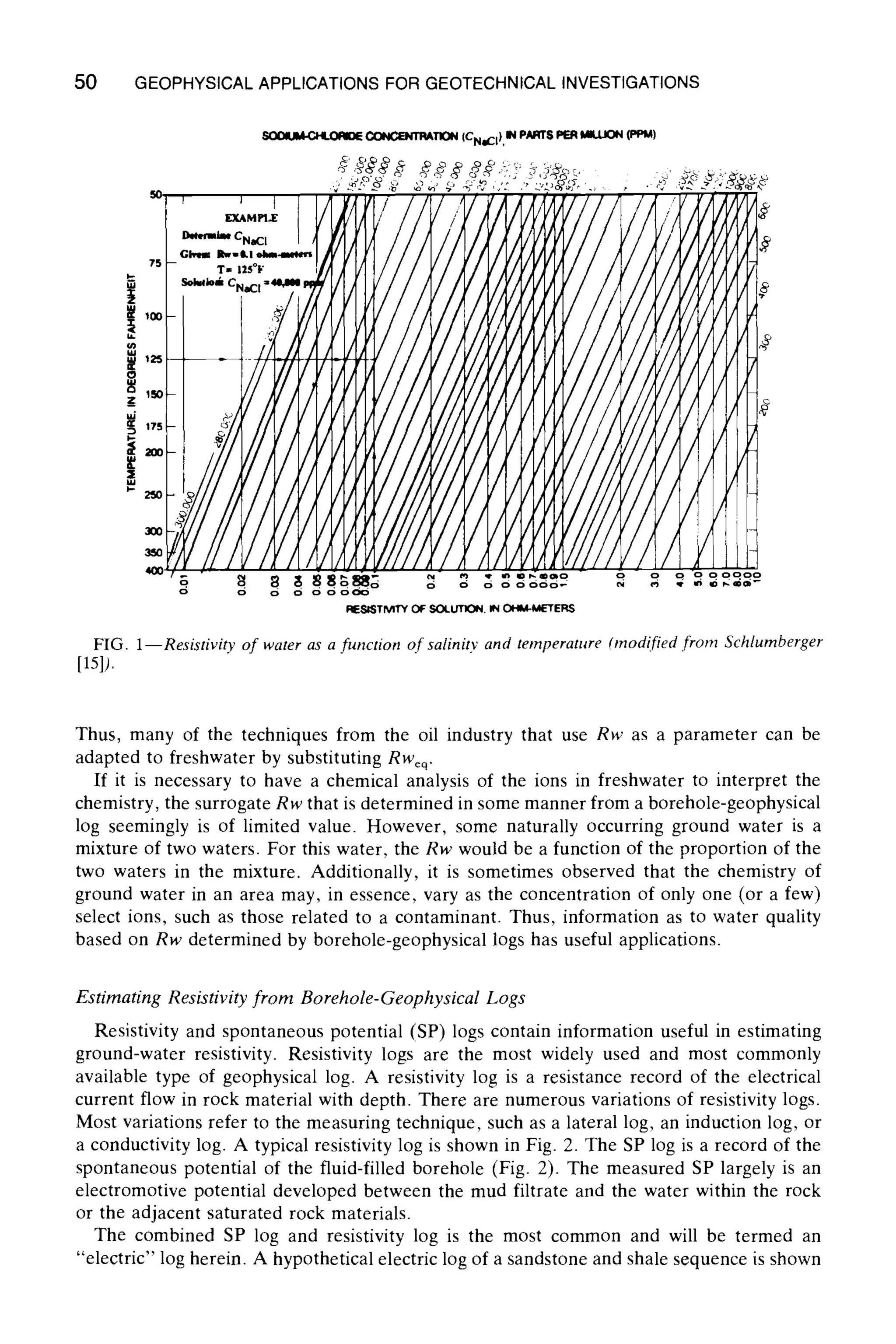
Rweq = Rw a Cfw (1)
CeqNaCl
where Cfw is the concentration of dissolved solids of the freshwater and Rwa is the apparent
Rw of the freshwater obtained by using values in Fig. 1 [15].
For example, if the sum of the concentration of the dissolved ions (dissolved solids
concentration) in a solution at 75~ (24~ is 500 ppm, the apparent resistivity of the water
(Rw~) would be 10 II 9m. If the sum of NaCI equivalent dissolved ions is 280 ppm, the
water resistivity of an equivalent NaCI solution would be:
RWeq = l0 X 500/280 = 17.6 f~" m](https://image.slidesharecdn.com/geophysicalapplicationsforgeotechnicalinvestigations-151104153926-lva1-app6892/75/Geotechnical-Geophysics-51-2048.jpg)
![JORGENSEN ON ESTIMATING WATER QUALITY 51
SPONTANEOUS
POTENTIAL
20+
~,~ ~g-MILLNOI.TS
,
.ES,STM~. I. O..-.ErERs ~rE~J.toa
Q2 ~.o ~o ,oo loooz ~o
m i I / i
z MEDIUM IND~ICTION
0.2 ~.o, ,o ,p ,~._~.
DEEP INOIJCTION
'l 0.2 ~O 10 100 1000 2r
t~
~Mecliumi~ tu~on
/,
2,000
..J
2,100-
pinduction./
FIG. 2--Electric logs (spontaneouspotential and resistivity) (fromJorgensen [6]).
in Fig. 3. Each deeper sandstone contains water of increased salinity. Two resistivity traces
are shown--a "deep" and a "shallow" trace. "Deep" implies the resistivity measurement
is of material at some distance from the well bore. In addition, it is commonly accepted
that deep resistivity measurements are more representative of undisturbed formation water
and rock. The "shallow" trace measures the resistivity of the material adjacent to the
borehole. Similarly, it is commonly accepted that this resistivity is most likely to be affected
by the invading drilling fluid. Several methods can be used to estimate water resistivity;
they are discussed below.
Qualitative Methods
Two little-known but easy-to-apply methods for qualitatively estimating relative water
resistivity use the resistivity log and the spontaneous potential log. Within Sandstone D,
the resistivity results as measured by both the shallow and deep traces are equal (Fig. 3).](https://image.slidesharecdn.com/geophysicalapplicationsforgeotechnicalinvestigations-151104153926-lva1-app6892/75/Geotechnical-Geophysics-53-2048.jpg)
![52 GEOPHYSICAL APPLICATIONS FOR GEOTECHNICAL INVESTIGATIONS
ELECTRICLOG
Spontaneouspotentia,_~Depth,~ Resistivity__
t Shale I i
t~-
SandstoneI
wmf I W=~ j
IS4mdmo~ T---"
ShakD Sat~eh~i I
fresh
,,,~ i __1 J
I Sa~ll /
/
D
,,w, I ~
FIG. 3--1dealized electriclog of shale and sandstone section containingfresh and saline water (from
Jorgensen [6]).
If invasion of drilling fluid occurs, the formation water resistivity can be assumed to be
equal to the invading fluid resistivity (mud filtrate) as measured by the shallow curve. If
the resistivity of the mud filtrate and the invading fluid are equal, then the formation water
resistivity is equal to the mud filtrate resistivity. Mud filtrate resistivity usually is measured,
and its value can be obtained by correcting the value reported on the log heading for
temperature. The unique condition described above is useful in quickly determining Rw at
one point and qualitatively evaluating Rw for the overlying and underlying aquifer material
if other factors affecting Rw are equal each formation.
Spontaneous potential (SP) largely is a function of the logarithm of the ratio of the ionic
activity of the formation water to the mud filtrate. Therefore, for the SP deflection to be 0
as shown for Sandstone D in Fig. 3, the ratio is 1 and the activities are equal. If resistivity
and ionic activities are assumed to be inversely proportional, which is the usual assumption
in interpreting SP logs, it follows that the resistivity of the water equals the resistivity of
the mud filtrate, which usually is recorded in the log heading. This unique condition is useful
in quickly estimating the water resistivity at one point and for qualitatively evaluating the
relative water resistivity in overlying or underlying permeable material if other conditions
are equal.
Spontaneous Potential Method
The two quantitative techniques typically used to estimate water resistivity are: (1) the
spontaneous potential method and (2) the cross-plot method. Both methods usually are](https://image.slidesharecdn.com/geophysicalapplicationsforgeotechnicalinvestigations-151104153926-lva1-app6892/75/Geotechnical-Geophysics-54-2048.jpg)
![JORGENSEN ON ESTIMATINGWATER QUALITY 53
presented in well-logging manuals and texts. However, information as to the accuracy of
the methods is not presented. The SP method is most commonly used and will be presented
first. A comparison of estimated to measured water resistivity values will be made to evaluate
the use and accuracy of the method.
The SP method is reported to be useful in estimating the resistivity of sodium chloride
water. The method is widely known and described in nearly all texts and well-logging
manuals, such as the Application of Borehole Geophysics to Water-ResourcesInvestigations
[16], and is based on the equation:
SP = - K log Rmf 2mrRw K log (2)
where SP is the spontaneous potential, in millivolts, at the in-situ or formation temperature;
K, in millivolts, is a constant proportional to its absolute temperature within the formation;
Rw is resistivity of water, in ohm-metres, at in-situ temperature; Rmf is the resistivity of
mud filtrate in ohm-metres; Aw is the ionic activity of the formation water; and Amf is the
ionic activity of the mud filtrate, also at the in-situ temperature. This method requires SP
values from an electric log and the mud filtrate resistance measurement, which usually is
recorded on the log heading. The SP value is the deflection difference between the shale
line and the adjacent permeable material and can be either positive or negative.
The SP method commonly is used because of the ready availability of SP logs (there are
more electric logs available than any other type of geophysical log). This method of estimating
water resistivity is reportedly useful in sand-shale sections in which good SP differences
exist, and, reportedly, it is not usable or works poorly in carbonate sections [17, p. 3].
However, the assumption that the SP method works poorly in carbonate is questionable
because no terms exist in Eq 1 that refer to lithology. The suitability of the method depends
on the SP difference not on a specific lithology.
An algorithm similar to the one presented by Bateman and Konen [18]for using SP to
determine Rw is shown in Fig. 4 [6]. Mud filtrate resistivity values (Rmf) at a specific
temperature (Tmf) and the in-situ temperature of the permeable material (Tf) at which the
SP is measured are necessary. The SP value, in millivolts, is the signed ( + or - ) difference
between the potential of the aquifer material and the potential at the reference shale line
(vertical line along which most shale or clay sections plot). If the value of Rmf is not known,
an estimate of Rrnf may be made from the mud resistivity (Rm):
Rmf ~ 0.75 nm (3)
The in-situ or formational temperature (Tf) is seldom known unless a temperature survey
has been made in the borehole sometime after drilling has been completed. However, 7f
may be estimated if the temperature between the mean annual temperature existing near
surface (Tma) and the temperature at the bottom of the borehole (BHT) is increased linearly
with depth; mathematically it can be shown as:
Tf ~ Tma + (BHT - Tma)(Df)
Dt (4)
where Dfis the formation depth and Dt is the total hole depth at which BHT was measured.
A second and similar method of estimating Tf uses information on the geothermal gradient
in degrees per unit depth of the area:
Tf ~ Tma + (geothermal gradient)(Df) (5)](https://image.slidesharecdn.com/geophysicalapplicationsforgeotechnicalinvestigations-151104153926-lva1-app6892/75/Geotechnical-Geophysics-55-2048.jpg)
![54 GEOPHYSICALAPPLICATIONSFOR GEOTECHNICALINVESTIGATIONS
Rm~, Tmt SP, "/']
L ,(Tml+7) g
Rm[75=RmI~ Rm[
Rmte
NO ~ YES Rra/75
,,.g, 146.mXTs-sl. ~ I . . . . 2_
_. I __ SP
K=00+0 133 TI
Rw~'-Rml~ lOSP/K T/
Tm]
I''~- ~ 12'~--I ..... )t
[ - - I
-- i
L .-=,-,,(8~/(T1+7)) I
EXPLANATION
Spontaneous potential constant at 9 opecl~ teml~rature
Resistivity of mud filtrate, in ohm-meters
Resistivity of mud filtrate equivalent, in ohm-m~ters
Rersistlvlty o| mud at 75"F. in ohm-meters
Reslstlvlly o| water, in ohm-meters
Resistivity of water equivalent, in ohm-meters
Resistivity of water at 75"F, in ohm-meteN
Spontaneous potential, in mlllivolts
TenpeTalvre ol Iormatlo~ in dcg~re~sFahre~helt ('F)
Temperature ol mud filtrate, in d ~ Fahrenlwit ('F)
FIG. 4--Spontaneous potentialmethod of estimating resistiritv of formation water ffrom Jorgensen
[61).
The procedure for the SP method to evaluate the water resistivity is:
1. Determine Rmf and Tmf. The values are read from the log heading. (If Rmf is not
available, estimate from Rm by using Eq 3.)
2. Determine SP from the spontaneous potential trace on the electric log.
3. Determine Tf from the temperature log or estimate by using either Eq 4 or Eq 5.
4. Determine the formation water resistivity (Rw) by using the algorithm shown in
Fig. 4.
Jorgensen [6] used the SP method to estimate Rw for eleven rock sections for which the
formation water resistivity had been measured. The eleven saturated rock sections tested
were mostly carbonates, which are reportedly not suitable for the SP method. No evidence
was observed to indicate that the method was better suited to sandstone than any other type
of rock material if the shale line for the SP curve could be established; however, only a few
sandstone rock sections were used in the test. Maximum or true static spontaneous potential
(SSP) is not always developed especially when the logged section includes thin layers of clay
and sand. Additionally, if there is considerable clay material in a sand, the log SP will not
represent the SSP.
Results of comparing the Rw estimated from the SP method versus the measured Rw
from the chemical analyses are shown in Fig. 5. A least-squares analysis for a linear relation
indicates a coefficient of determination (r2) of 0.66 for the SP data. A coefficient of deter-
mination of 0 indicates no correlation, and a value of 1 indicates perfect correlation. The
value of 0.66 indicates that some correlation exists. A scatter of about one order of magnitude
might be expected, as shown in Fig. 5. The coefficient of determination of 0.66 may be
typical for the method if the logs usually available from the petroleum industry are used.
This might be interpreted as a very inaccurate estimator of resistivity. However, water](https://image.slidesharecdn.com/geophysicalapplicationsforgeotechnicalinvestigations-151104153926-lva1-app6892/75/Geotechnical-Geophysics-56-2048.jpg)
![JORGENSEN ON ESTIMATINGWATER QUALITY 55
100
o_ I
>_
c~ 1.0-
.=,
0.1--
==
0.01
0.01
I
Method of Delermination
Cross pie!
o Spontaneous potential
I i
,~15
z~3
~1 ~4 ~12 0 2
91o~2 o3 ~ ~13o4
8~, o~.14 6~10
5~,7
8,9 ~ ~ o12
I I I
0.1 1.0 10
MEASUREDWATERRESISTIVITY,IN OHM-METERS
lO0
FIG. 5--Measured and estimated resistivity of water (from Jorgensen [6]).
resistivity that occurs in nature ranges from about 0.01 to more than 10 Ft 9m or more than
three orders of magnitude. Thus, for areas that have no measured data and if an estimate
of water resistivity of plus or minus a half order of magnitude is an acceptable range of
accuracy, the method may be used with caution. If additional information from a chemical
analysis of water at a specific zone in the logged hole is available, the correlation between
water resistivity and SP responses can be greatly improved as was demonstrated by Alger
[9].
The accuracy of the method is dependent on the accuracy of the SP measurement. Spon-
taneous potential is difficult to measure accurately because spurious electromotive forces
inadvertentlyare included in the measurement. Equation 2 is most applicable if the formation
water is saline, sodium and chloride are the predominant ions, and the mud is relatively
fresh and contains no unusual additives.
Because water resistivity is a surrogate water quality parameter, its relation to the water
chemistry parameter of interest should be considered in any evaluation of its value as a
water chemistry indicator. For example, Fig. 1 shows that the relation between the con-
centration of NaC1 and resistivityis inverse and not linear. The accuracy of Rw as an indicator
of NaC1 concentration depends on what log cycle Rw exists in, as also shown in Fig. 1.
Cross-Plot Method
The cross-plot method is reported in most logging texts and manuals; however, little or
no discussion is made of the accuracy of this method. The method is discussed in some
detail by MacCary [19]. The cross-plot method is sometimes referred to as the "carbonate"
method or the "Pickett" cross-plot method. This method is not as widely used as the
previously discussed SP method because it requires one or more porosity logs in addition
to a resistivity log.
As the name indicates, the method is based on a cross plot of resistivity and effective
porosity values. (Unless specified otherwise, porosity reported herein is effective or inter-
connected porosity.) Values of porosity and resistivity of saturated material are plotted on](https://image.slidesharecdn.com/geophysicalapplicationsforgeotechnicalinvestigations-151104153926-lva1-app6892/75/Geotechnical-Geophysics-57-2048.jpg)
![56 GEOPHYSICALAPPLICATIONS FOR GEOTECHNICAL INVESTIGATIONS
log-log graph paper and a line is fitted to the points. Ideally, the points will define a straight
line, and the intercept of the line projected to the 100% porosity value would represent the
Rw. Assuming Archies law is applicable, this hypothesis was tested using data from two
carefully conducted tests on limestone cores (DC & FA #1 and Geis #1) from Douglas and
Saline Counties, Kansas. The cores were saturated with water of a known resistivity. The
results, as shown in Fig. 6, were useful because the projection of a line that fitted most of
the data from the Geis #1 core intercepted the 100% porosity line close to the measured
Rw value. However, DCA & FA #1 core results show that most or nine of eleven data
points fall below the straight line, probably because the Ro values for porosity values less
than 3% may be affected by surface conductance along the grains. (Ro is the combined
resistance of water and the saturated rock.) For formations saturated with freshwater,
Archies law, which is based on the assumption that the matrix is nonconductive and that
surface conductance along grains and ionic exchange are slight, is not accurate. However,
the cross-plot method of observed log resistivity values plotted against porosity values still
should define a curve, which projected to the 100~k porosity intercept will define Rw.
Porosity and resistivity values for the cross plot can be obtained from geophysical logs.
Homogeneous lithology, constant water resistivity, and 100% water saturation are assumed.
Logging devices that "look deep" into a formation provide better Ro values. Suitable logs
might be a deep-induction log (as shown in Fig. 2), a long-lateral log, a deep-conductivity
log, and so forth. (Conductivity is the inverse of resistivity, generally recorded in units of
milliohms per metre or microohms per metre, on geophysical logs.)
Porosity values are best determined from a dual-porosity log (density and neutron), such
as the log shown in Fig. 7. However, other single-porosity logs, such as sonic, neutron,
density, or dielectric logs, could also be used. Porosity determinations using a resistivity log
cannot be used.
100
10
Z
s
1.0
o
Is PL~A130N
D DC~FA BI, Core, doloaoee
o Ge~ 9 I, Core, dokxaoee
x Meamared water r~detNtty
m Cementltlcm (actor
o.1 I 1 I
0.1 1.0 1 0 100 1,00~
RIESlSTfVITYOF ROCK WATER SYSTEM (Ro), I~NOHM-METERS
FIG. 6--Cross plot of resistivity and porosity measured on dolostone cores (from Jorgensen [6]).](https://image.slidesharecdn.com/geophysicalapplicationsforgeotechnicalinvestigations-151104153926-lva1-app6892/75/Geotechnical-Geophysics-58-2048.jpg)
![JORGENSEN ON ESTIMATING WATER QUALITY 57
CALIPER ~ i POROSITY.IN PERCENT(LIMESTONEMATRIX)
DIAMETERIN INCHES 13 i COMPENSATEDFORMATION-DENSfTYPOROSITY
GAMMARAY,INAPi UNITS Z ~_ 20 10 0 "10
150 ~ I COMPENSATED-NEUTRONPOROSITY
300 ~ 130 20 lo o -1090 ~ ~ ........................L
j 1,900 '
ii I
~'Caliper l
r i
I
I'
_-
,~Gamma ray
_
P
__ L
2,000
i
i
+] 2,100
i
iI
i
I
i
Sandstone
i -)
Densityporosity~ ~ ~.
i !% 5
i ~Neutron Porosity
FIG. 7--Dual porosity, gamma-ray, and caliper logs (from Jorgensen [6]).
When the cross-plot procedure is used after determining porosity with a graph like
Fig. 8, it is not always possible to select points defining a straight line to the degree of
desired accuracy. Logs that have expanded depth scales are more easily used in selecting
suitable porosity and resistivity value sets because it is possible to locate the same point on
all the logs more accurately. An example of the method is shown in Fig. 9. The data plotted
in Fig. 9 were picked from the logs shown in Figs. 2 and 7.
If the rock section is not 100% saturated with water, the rock-water system resistivity
(Ro) values obtained from the log will be larger than the Ro values of the aquifer material
if it had been 100% saturated. The values would plot to the right of the line defining n
compared to Ro for a 100% water-saturated section. The unusually large resistivity values
may indicate an unsaturated zone, hydrocarbons, gases, or unconnected porosity. Unusually
small resistivity values might indicate that clay minerals occurred in some rock sections.
Because the cross plot of porosity and resistivity logarithms defines a straight line, standard
least-squares techniques can be applied to determine the standard estimate of error. Ac-](https://image.slidesharecdn.com/geophysicalapplicationsforgeotechnicalinvestigations-151104153926-lva1-app6892/75/Geotechnical-Geophysics-59-2048.jpg)
![58 GEOPHYSICAL APPLICATIONS FOR GEOTECHNICAL INVESTIGATIONS
2o]
~Sulfur
] ~s=,
221
,,=,
2.3,-
o=
2.4;
'
2.6
== i
2 7 ~
i
28!
i
301
FRESHWATER,LIQUID-RLLEDHOLES
i
i
EXkMPI.E
D~emmlM Porosi~r(;i~en:
nS=9
n~=t9
n=14
dl'l 0
Langm~eirtitli
&
Polyhliitl
tJ
o m ~o -3o
PO~IOSITYFROM NEUTRON LOG (nn), IN PERCENT (APPARENTLIMESTONE POROSITY)
24o
d
~2s
w
-2o~.
x
E'o ~,
-- 8
:o g=
~-10
4
~-15
FIG. 8--Porosity and lithology from the formation density log and compensated neutron log (modified
from Schlumberger [20]).
cordingly, the standard estimate of error for Rw can also be defined. Note the estimated
Rw that is determined is for formation conditions.
Jorgensen [6] tested the accuracy of the method by estimating Rw for 15 rock sections
for which Rw had been measured. The coefficient of determination of 0.88 was determined
from a least-squares analysis. The value of 0.88 may be typical of estimates that are based
on usually available logs. Inspection of Fig. 5 shows variations or scatter of about one order
of magnitude in a range of more than three orders of magnitude that can be expected in
nature. Thus, based on the results shown in Fig. 5, the method did not accurately estimate
Rw; however, the method can be used to estimate formation water resistivity for areas that
have no data if an estimated accuracy of plus or minus a half order of magnitude is acceptable.
The accuracy of the method is, in general, proportional to the extent of the range in
porosity that is measured within the section of interest. The wider the range, the more
accurately the line can be defined. Accuracy of reading the recorded measurement from
the log (trace) is improved if the scale is expanded.](https://image.slidesharecdn.com/geophysicalapplicationsforgeotechnicalinvestigations-151104153926-lva1-app6892/75/Geotechnical-Geophysics-60-2048.jpg)
![Q.
_Z
O
o_
JORGENSENON ESTIMATINGWATERQUALITY 59
Dala Deplh, R,.
poml mleet tf.g2l(hg7
10--
1 2,020 g 5 g 5
2 2026 12 10
3 2.036 18 6
4 2,041 26 3 5
5 2059 6 13
6 2.071 45 16
j 7 2.0~2 6 7
0 ~ L _ ~0
o h m - m e t e r s ~
EX J,'~lI'I,FZ
Determine: Waterre$tstivtty(Rw),r factor(rn),
and formationtemperature(Tt)
Given: Geothermaigradient=6.0[33~Fahrenheii
6 perfoot
Averagedepth= 2055 feet
1c2 o
P Meanannualtemperature=55 Fshrenhelt -
~7 ~ Solution: Rw=Ro at |O0-percentpor =0.38
rn~ 1.37/I = 1.37
Fahrenheit
RESISTIVITY OF THE RCCK-WATER SYSTEM (Ro). IN OHM-METERS
FIG. 9--Cross plot of geophysical log values of Ro and n (from Jorgensen [6]).
The Rw value may be used to estimate water chemistry if the relation has been established.
For example, the sodium chloride content can be estimated for many saline waters if the
in-situ temperature of the water is available or can be estimated. Turcan [13] used resistivity
logs to determine Rw, which were in turn correlated with chloride or dissolved solids con-
centrations. Turcan's analysis indicates that a high degree of correlation can be established
if some water chemistry data are available.
The dissolved solids concentration can be estimated from specific conductance (conduc-
tance at 75~ [24~ usually in units of microsiemens or micromohs per centimetre, if the
relation between the specific conductance and dissolved solids is known. A method of
estimating the dissolved solids concentration in water from specific conductance is given in
Appendix A.
Formation Factor Methods
Sethi [21] presented a comprehensive review of the work of many researchers in defining
formation factor relations. The relation of rock resistivity, water resistivity, porosity, and
tortuosity were first described by Archie [22, p. 56]. Archie, assuming that rock was non-
conductive, gave:
F = n-" (6)
where F is the formation factor (dimensionless), n is porosity (dimensionless), and m is the
cementation factor (dimensionless).
The relation of the formation factor to pressure and temperature is not completely known.
In reference to the temperature effect, Somerton [23, Fig. 12, p. 188] showed that the
logarithm of the ratio of the formation factor at a specific temperature to the formation
factor at a specified reference temperature for the Mississippian Berea Sandstone varied
nonlinearly with temperature change.](https://image.slidesharecdn.com/geophysicalapplicationsforgeotechnicalinvestigations-151104153926-lva1-app6892/75/Geotechnical-Geophysics-61-2048.jpg)
![60 GEOPHYSICALAPPLICATIONSFOR GEOTECHNICALINVESTIGATIONS
For increasing pressure, Helander and Campbell [24, p. 1], in relation to the formation
factor, report: (1) the formation factor changes as the mean free path for current increases
as constriction closes pores; (2) the degree of constriction, which causes change of the
formation factor, is mostly due to the closing of the smallest pores; and (3) the effect of the
double layer on the formation factor is increased as the pore throat areas decrease with
decreasing porosity.
The cementation factor (m) largely is a function of tortuosity and pore geometry. Tor-
tuosity is the ratio of the fluid path length to the sample length. Aquilera [25] studied the
effect of fractured rock on the formation and cementation factor. He used a double-porosity
model in defining m. The model development implies that m will be near to 1 for a rock
mass in which all porosity is the result of fractures (that is. there is no interconnected primary
porosity). Because the length of the flow path in a fractured medium is much shorter than
the length of the flow path in a porous medium, the tortuositv of the fractured medium is
relatively small, and the cementation factor also is small and is near to 1. The relation of
porosity (n), the formation factor (F), and the tortuosity factor (T)of Bear [26, p. 115] is:
1
F = Tnn (7)
where Tis the square of the ratio of the length of the sample to the length of the electrical
flow path. Archie [22] further defined:
F = Ro/Rw (8)
where Ro is resistivity observed (log resistivity) and Rw is the formation water resistivity.
(Herein, Ro is assumed to be the bulk water and rock resistivity unaffected by fluid invasion,
sometimes termed true resistivity or Rt.)
Accordingly, an estimate of Rw can be made if F is known and a measurement of Ro is
available because:
Rw = Ro/F (Sa)
For example, if Eqs 6 and 8a are combined, the equation becomes:
Rw = Ro n" (9)
If Rw is constant, Eq 9 will produce a straight line with the slope of -m on a log-log plot
of n versus Ro.
Techniques or methods that produce a formation factor can be used to estimate an Rw
value. Pirson [27, p. 24] relates for "clean" rock:
Rxo
F ~ .... (10)
Rmf
where Rxo is the resistivity of the invaded zone of the porous formations around the well
bore. Rxo can be obtained from a microresistivity log, "laterolog 8," spherically focused
micro-laterolog, or a "proximity" log and sometimes a short normal. Rmf is a resistivity
measurement of the mud filtrate. Combining Eqs 8 and 10 yields:
Rw ~ Ro Rmf (11)
Rxo](https://image.slidesharecdn.com/geophysicalapplicationsforgeotechnicalinvestigations-151104153926-lva1-app6892/75/Geotechnical-Geophysics-62-2048.jpg)
![JORGENSEN ON ESTIMATING WATER QUALITY 61
Equation 11 is a useful indicator because all terms are available from a suite of modern
resistivity logs.
In aquifers that contain very fresh water (Rw greater than 10 ~ - m), the formation factor
assumptions of Archie [22] are inaccurate. This is because the resistivity of the saturated
formation is in part a function of surface conductance along the grains and ionic exchange
between the rock grains and water. Additionally, formation factor relations for the for-
mations that have significant clay or shale content may differ from the Archie relations.
Accordingly investigators, such as Biella et al. [7] use an apparent formation factor concept.
Jorgensen [28] and some other investigators have correlated F with intrinsic permeability,
porosity, and the cementation factor. Thus, if permeability and other properties, such as
porosity, the cementation factor, and observed log resistivity, are available, Rw can be
estimated. These methods, however, are beyond the scope of this paper.
Summary
Borehole-geophysical logs can be used to provide information on water quality. Most
information is obtained indirectly from various geophysical logs. Little information can be
obtained by direct measurement of water quality properties. However, in water wells, direct
measurements of chloride, dissolved oxygen, pH, and water conductivity are sometimes
made by using special borehole-geophysical probes.
Most geophysical logs are made in test holes filled with drilling fluid. Geophysical logs
in test holes measure properties, such as combined water and rock resistivity values, which
can be related to water quality. Relations between water resistivity and water chemistry
enable data from borehole-geophysical logs to be correlated to water chemistry.
Water resistivity largely is a function of water chemistry and temperature. In freshwater
aquifers, resistivity is inversely proportional to the activity of ions, such as Ca + +, Mg ++,
SO4 , CO3 , and HCOs as well as Na + and C1-. (This is the usual case for most water
wells.)
In most deep boreholes, such as those used for petroleum exploration, saline water is
encountered in which sodium and chloride are the dominant ions. Accordingly, the oil
industry has developed many interpretive techniques based on relations among sodium
chloride concentration, dissolved solids concentration, temperature, and resistivity. Many
of these techniques can be used in freshwater aquifers if the resistivity of an equivalent
NaC1 solution can be determined.
The spontaneous potential (SP) log along with a resistivity log can be used to determine
Rw from the equation
SP = - K log(Rmf/Rw)
Rw also can be determined from a cross plot of observed log resistivity and porosity.
Values of Ro are read from deep-looking resistivity logs, and porosity is determined from
logs, such as neutron, gamma-gamma, sonic, and dielectric logs. The slope of the plot is
the negative of the cementation factor (- m).
The SP method and the cross-plot method of estimating Rw are both crude estimators
because an accuracy of plus or minus a half order of magnitude may result. However,
because naturally occurring resistivity values are in a range of about three orders of mag-
nitude, estimates of Rw may be useful if data are scarce. If additional data, such as a
chemical analyses, can be correlated to a log, accuracy of estimates is greatly increased.
The concept of the formation factor (F) relates porosity (n), the cementation factor,](https://image.slidesharecdn.com/geophysicalapplicationsforgeotechnicalinvestigations-151104153926-lva1-app6892/75/Geotechnical-Geophysics-63-2048.jpg)
![62 GEOPHYSICALAPPLICATIONS FOR GEOTECHNICAL INVESTIGATIONS
resistivity water (Rw) observed log resistivity of the formation material (Ro), resistivity of
mud filtrate (Rmf), and resistivity of invaded zone (Rxo). The equations are:
F = Ro/Rw -~ Rxo/Rmf
and
Rw = Ro nm
Logs such as "formation factor" logs and microresistivity logs can be used to estimate F
or Rw or both.
Acknowledgments
The impetus for this study was the need for water quality information for aquifers for
which few data are available. The study was made as part of the U.S. Geological Survey's
Regional Aquifer System Analysis Program. The assistance and encouragement of Fred
Paillet, U.S. Geological Survey, Denver, Colorado; George Asquith. Mesa Operating Lim-
ited Partnership, Amarillo, Texas; and John Doveton, Kansas Geological Survey, Lawrence,
Kansas, are appreciated. Data and information provided by Alan Duton, Bureau of Eco-
nomic Geology, Austin, Texas; Schlumberger Co.. Houston, Texas: and the U.S. Geological
Survey offices in Lawrence, Kansas. and Denver. Colorado, were essential to the study.
APPENDIX A
Estimating the Dissolved Solids Concentration
The dissolved solids concentration can be estimated from resistivity or specific conductance meas-
urements. Specific conductance is a measure of the conductance of electrical current through a fluid
and usually is expressed in units of microsiemens or micromhos per centimetre. A specific conductance
measurement is referenced to a specified temperature, usually 25~ (77~
Specific conductance in microsiemens per centimetre, which is the resistivity reciprocal at 25~ (77~
can be calculated from the equation (Jorgensen [6]):
1 x 10⁴
SC - - - (A1)
RW77
where Rw77is the water resistivity at 25~ (77~ in ohm-metres.
Resistivity of water (Rw• at any temperature, (Tx) in degrees Fahrenheit, can be converted to Rwv7
by the Arps equation [29]:
(Tx + 7)
Rw77 = R w ~ - [61 (A2)
84
The resistivity of water (Rw• at any temperature x (Tx) in degrees Fahrenheit can be calculated if
the resistivity of that water at temperature y (Ty) is known:
RwX = Rw, Ty + 7 (A3)
rx+7
The relation between the dissolved solids concentration, in parts per million (ppm), and specific
conductance, in microsiemens per centimetre, is:
DS ~ (P) (SC) (A4)](https://image.slidesharecdn.com/geophysicalapplicationsforgeotechnicalinvestigations-151104153926-lva1-app6892/75/Geotechnical-Geophysics-64-2048.jpg)
![JORGENSEN ON ESTIMATINGWATER QUALITY 63
where P is a factor to be determined for each water but typically is about 0.67 for many ground waters
if specific conductance is in units of microsiemens per centimetre [6].
The dissolved solids concentration also can be estimated from the sodium chloride concentration.
The empirical relation between sodium chloride concentration (CNao) and dissolved solids concentration
(DS) is:
DS ~ (A) (CNaCI) (A5)
where DS and Cnac~ are both in the same units. The coefficient A needs to be determined for each
water type; however, the value of A has been determined to be about 1.04 for many natural waters
[6].
APPENDIX B
Estimating Sodium Chloride Concentration
Many useful interpretations of geophysical log data are based on relations for sodium chloride
solutions. Relations among water resistivity, temperature, and dissolved solids concentration are shown
in Fig. 1 and reported by Jorgensen [6]. Most of the curves on Fig. 1 can be approximated by the
equation:
CNaCl,ppm ~ (2500/Rw75) Hz5 (BI)
where CNaCl,ppm is the sodium chloride concentration in parts per million and Rw75is the resistivity in
ohm-metres of the solution at 75~ (23.8~ which is the usual reference temperature in geophysical
logging.
Values of resistivity, in ohm-metres, at any temperature, Tx, in degrees Fahrenheit, can be converted
to resistivity at 75~ (23.8~ by the equation:
Rw75 = (RWx) (Tx + 7)/(82) (B2)
Sodium chloride concentration, in milligrams per litre (mg/L) can be converted to concentration in
parts per million by:
CNaCl,ppm = (CNaCI,mg/L)/(G) (B3)
where G is specific gravity and is the solution density divided by pure water density.
Concentration of a sodium chloride solution in milligrams per litre (CNao,mgm) can be converted to
estimated concentrations in parts per million (CNao,ppm) by the following equations
CNaCi,ppm ~ CNaCI,mWL/(1 + 6.7 • 10 -7 CNaCI,mg/L) (B4)
Investigators, such as Alger [9], Turcan [13],and Desai and Moore [14],list multipliers that enable
resistivity of equivalent sodium chloride solutions to be estimated for solutions that contain ions other
than Na and C1.
References
[1] Doveton, J. H., Log Analysis of Subsurface Geology--Concepts and ComputerMethods, John
Wiley, New York, 1986.
[2] Hearst, J. R. and Nelson, P. W., WellLoggingof PhysicalProperties, McGraw-Hill, New York,
1985.
[3] Log InterpretationPrinciples~Applications, Schlumberger Educational Services, Houston, Texas,
1987.
[4] Log InterpretationFundamentals,Dresser Atlas, Houston, Texas, 1975.](https://image.slidesharecdn.com/geophysicalapplicationsforgeotechnicalinvestigations-151104153926-lva1-app6892/75/Geotechnical-Geophysics-65-2048.jpg)
![64 GEOPHYSICAL APPLICATIONS FOR GEOTECHNICAL INVESTIGATIONS
[5] Keys, W. S., "Borehole Geophysics Applied to Ground-Water Investigations," U.S. Geological
Survey Open-File Report 87-539, 1988.
[6] Jorgensen, D. G., "Some Uses of Geophysical Logs to Estimate Porosity, Water Resistivity, and
Intrinsic Permeability," U.S. Geological Survey Water-Supply Paper 2321, 1989.
[7] Biella, G., Lozei, A., and Tabacco, I., "Experimental Study of Some Hydrogeophysical Properties
of Unconsolidated Porous Media," Ground Water, Vol. 21. No. 6, 1983. pp. 741-751.
[8] Jones, P. H. and Buford, T. B., "Electric Logging Applied to Ground-Water Exploration,"
Geophysics, Vol. 16, No. 1, 1951, pp. 115-139.
[9] Alger, R. P., "Interpretation of Electric Logs in Fresh Water in Unconsolidated Formations,"
Transactions of the 7th Annual Logging Symposium, Society of Professional Well Log Analysts,
Tulsa, OK, 1966, pp. CC1-CC25.
[10] Pfannkuch, H. O,, "On the Correlation of Electrical Conductivity Properties of Porous Systems
with Viscous Flow Transport Coefficients," paper presented at First International Symposium of
the Fundamentals of Transport Phenomena in Porous Media, International Association Hydraulic
Research, 1969, pp. 42-54.
[111 Worthington, P. F., "Hydrogeophysical Equivalence of Water Salinity. Porosity, and Matrix Con-
duction in Arenaceous Aquifers," Ground Water, Vol. 14. No. 4. 1976, pp. 224-232.
[12] Urish, D. W., "Electrical Resistivity-Hydraulic Conductivity Relationships in Glacial Outwash
Aquifers," Water Resources Research, Vol. 17. No. 5. 1981. pp. 1401-1408.
[13] Turcan, A. N., Jr., "Calculation of Water Quality from Electrical Logs--Theory and Practice,"
Louisiana Geological Survey Water Resources Pamphlet 19. 1966.
[14] Desai, K. P. and Moore. E. J., "Equivalent NaCI Solutions from Ionic Concentrations," Log
Analyst, Vol. 10, No. 3. 1969.
[15] Log Interpretation, Volume 1--Principles, Schlumberger Limited. New York. 1972.
[16] Keys, S. W. and MacCary. L. M.. "Application of Borehole Geophysics to Water-Resources
Investigation,'" U.S. Geological Survey Techniques qf Water-Resources Investigations, Bk. 2, U.S.
Geological Survey, 1971, Chap. El.
[17] MacCary, L. M., "Use of Geophysical Logs to Estimate Water-Quality Trends in Carbonate
Aquifers," U.S. Geological Survey Water-Resources Investigation Report 80-57. 1980.
[18] Bateman, R. M. and Konen, C. E., "The Log Analyst and the Programmable Pocket Calculator,"
Log Analyst, Vol. 18, No. 5, 1977, pp. 3-10.
[19] MacCary, L. M., "Interpretation of Well Logs in a Carbonate Aquifer.'" U.S. Geological Survey
Water-Resources Investigation Report 78-88, 1978.
[20] Log Interpretation Charts, Schlumberger Well Surveying Corp., Houston, 1979.
[21] Sethi, D. K., "Some Consideration about Formation Resistivity Factor-Porosity Relations," 20th
Annual Logging Symposium, Transactions of Society Professional Well Log Analysts, 1979.
[22] Archie, G. E., "The Electrical Resistivity Log as an Aid in Determining Some Reservoir Char-
acteristics," American Institute of Mining and Metallurgical Engineers Transactions, Vol. 146, 1942,
pp. 54-62.
[23] Somerton, W. H.. "Porous Rock-Fluid Systems at Elevated Temperatures and Pressures.'" Geo-
logical Society of America Special Paper 189, 1982, pp. 183-197.
[24] Helander, D. P. and Campbell, J. M., "The Effect of Pore Configuration, Pressure, and Tem-
perature on Rock Resistivity," Transactions of 7th Annual Logging Symposium, Society Profes-
sional Well Log Analysts, 1966.
[25] Aquilera, R., "Analysis of Naturally Fractured Reservoirs from Conventional Well Logs," Journal
of Petroleum Technology, Vol. 28, 1976, pp. 764-772.
[26] Bear, J., Dynamics of Fluids in Porosity Media, Elsevier. New York. 1972.
[27] Pirson, S. J., "Quick Qualitative Wellsite Log Evaluation with the Rxo/Rt Curve," Log Analyst,
Vol. 19, No. 1, 1978, pp. 21-25.
[28] Jorgensen, D. G., "Estimating Permeability in Water-Saturated Formations," Log Analyst, Vol.
29, No. 6, 1988, pp. 401-409.
[29] Arps, J. J., "The Effect of Temperature on the Density and Electrical Resistivity of Sodium
Chloride Solutions," Journal of Petroleum Technology, Vol. 5, No. 10, Section 1, Technical Note
195, 1953, pp. 17-20.](https://image.slidesharecdn.com/geophysicalapplicationsforgeotechnicalinvestigations-151104153926-lva1-app6892/75/Geotechnical-Geophysics-66-2048.jpg)
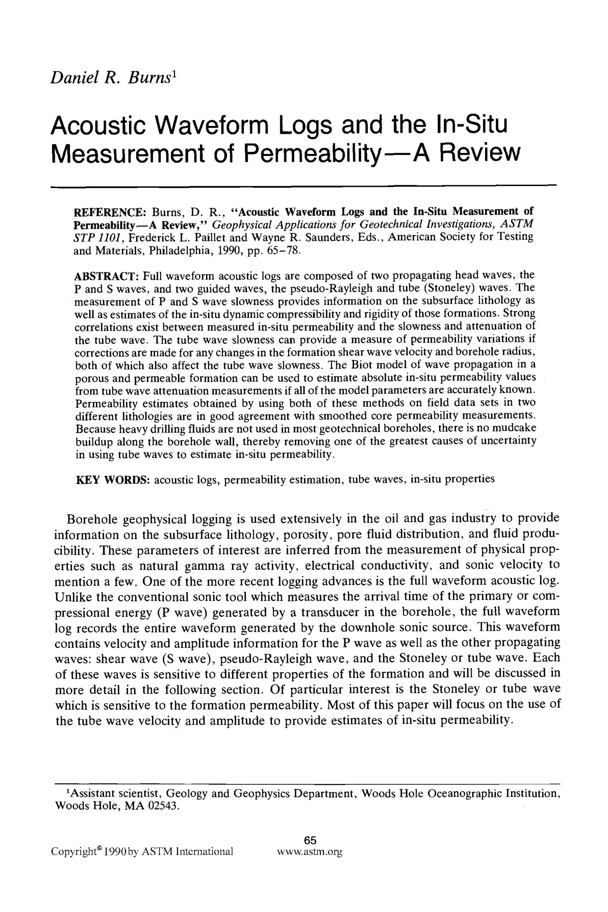
![66 GEOPHYSICALAPPLICATIONSFOR GEOTECHNICALINVESTIGATIONS
Full Waveform Acoustic Logs
The conventional full waveform acoustic logging tool consists of an axisymmetric source
and two or more receivers. The source generates a pressure pulse in the 1- to 20-kHz range
within the fluid contained in the borehole. The waveform at each receiver is recorded for
later velocity and amplitude analysis. These logs can also be run in air-filled boreholes, but
this paper will only treat the fluid-filledborehole situation. In air-filled holes, the wave types
and relationships will be somewhat different.
In fluid-filled boreholes, the waveforms generally consist of four arrivals: the P wave, the
S wave, the pseudo-Rayleigh wave, and the Stoneley (tube) wave. The P wave corresponds
to energy which is critically refracted along the borehole wall and propagates at the P wave
velocity of the formation. Leaky P waves arrive after the initial P wave energy and before
the S wave energy. These waves correspond to compressional energy that is partially trapped
in the borehole and can be conceptually thought of as acoustic energy reverberating inside
the borehole which generates compressional head waves in the formation each time it hits
the borehole wall [1,2].
The S wave is generated when the pressure pulse in the fluid is critically refracted as shear
energy at the borehole wall. The S wave propagates at the shear wave velocity of the
formation, but the amplitude of this arrival is very small and it is usually overwhelmed by
the larger amplitude pseudo-Rayleigh wavetrain.
The pseudo-Rayleigh wave represents the constructive interference of a Rayleigh wave
in the formation and reflected pressure waves inside the borehole [3]. This wave is dispersive,
but its first arrival (low frequencies) travels at the shear wave velocity of the formation. At
higher frequencies, the velocity approaches the P wave velocity in the fluid. Any number
of pseudo-Rayleigh modes can exist, corresponding to the fundamental and harmonic res-
onances of the borehole, although only one or two are generally present for the normal
frequency range used in logging.
The final propagating wave is the Stoneley or tube wave. The Stoneley wave is a slightly
dispersive surface wave which propagates along the borehole wall. It propagates at a velocity
less than the lowest velocity of the fluid or formation. In hard rock situations, the Stoneley
wave velocity is less than the borehole fluid velocity. In soft rock settings, however, the
velocity is less than the shear wave velocity of the formation. The Stoneley wave behavior
will be more fully described in later sections.
Figure 1 is a schematic of the propagation behavior of the major wave types.
The difference between soft and hard rock settings is a quantitative one. A hard formation,
also known as a fast formation, refers to the situation in which the shear wave velocity of
the formation is greater than the sonic velocity in the fluid. In these cases, shear waves can
be critically refracted at the borehole wall, and all wave types will be generated. A soft
formation (or slow formation), on the other hand, refers to the case in which the formation
shear wave velocity is less than the fluid sonic velocity. In this situation, shear energy cannot
be critically refracted at the borehole wall, and therefore no S or pseudo-Rayleigh wave is
generated, only the P and Stoneley waves exist. In each of these situations, the wave types
are sensitive to certain properties of the formation and borehole fluid. Figure 2 shows a
typical recorded trace obtained in hard and soft formation situations, with the different wave
types identified. More detailed descriptions of the various wave types and their propagation
behavior can be found in the literature [1-3].
Formation Properties
In addition to the sensitivity of the Stoneley wave to permeability variations, each of the
propagating waves are sensitive to other properties of the formation and borehole fluid. In](https://image.slidesharecdn.com/geophysicalapplicationsforgeotechnicalinvestigations-151104153926-lva1-app6892/75/Geotechnical-Geophysics-68-2048.jpg)
![BURNS ON ACOUSTIC WAVEFORM LOGS 67
R i
T
R
p
.~/fl
/ $
3" ,
t
r
t
P-Leaky P Wave S; pseudo-Ray|eigh Waves Tube Wave
FIG. 1--Schematic diagram of the acoustic modes that propagate in a borehole. T and R refer to the
transmitter and receiver positions, respectively.
hard rock situations, the P wave provides a measure of the P wave velocity of the formation,
and the pseudo-Rayleigh wave provides a measure of the shear wave velocity of the for-
mation. These velocity values, together with density information obtained from other meas-
urements, can provide estimates of the dynamic compressibility and rigidity of the subsurface
formations. P and S velocity can also be used to help identify lithologic variations in the
subsurface [4]. The velocity and amplitude of the Stoneley wave in these situations are most
sensitive to the borehole fluid properties and the formation permeability. To a lesser degree,
the Stoneley wave is also sensitive to the formation shear wave velocity. All of the waves
TUBE
PSEUDO-
p r RAYLEIGH 1
I FAST BAND
TUBE
P f 1
i i FLUID
ARRIVAL
O 8.75
TIME (msec)
FIG. 2--Example offull waveform acoustic log datafrom a "fast" and "slow" formation (also referred
to as "'hard" and "soft" formations). The arrivals are identified on each trace (after Williams et al. [13]).](https://image.slidesharecdn.com/geophysicalapplicationsforgeotechnicalinvestigations-151104153926-lva1-app6892/75/Geotechnical-Geophysics-69-2048.jpg)
![68 GEOPHYSICAL APPLICATIONS FOR GEOTECHNICAL INVESTIGATIONS
can be greatly affected by changes in the borehole diameter, such as those caused by
washouts. When using the Stoneley wave to estimate permeability variations, these other
factors that can affect its behavior must be kept in mind.
When full waveform acoustic log data is collected in a soft or slow formation, such as
might be expected in shallow, poorly consolidated sediments, the sensitivity of the arrivals
is much different. In soft formations, the P wavetrain becomes longer in duration and higher
in amplitude relative to the other arrivals. The P wave arrival still provides a measure of
the formation P wave velocity. The amplitude of the wavetrain, however, becomes much
more sensitive to the Poisson's ratio of the formation (and hence the shear wave velocity
of the formation) [1]. As mentioned above, no S or pseudo-Rayleigh waves are generated
in soft formation situations, so no direct measure of the formation shear wave velocity is
possible from the data. The Stoneley wave. however, is very sensitive to the formation shear
wave velocity (Vs)in this case and can be used to obtain an estimate of (Vs) [5]. The Stoneley
wave is also sensitive to formation permeability and variations in the borehole diameter.
The discussion up to this point has focused on the velocity of the different wave types.
The amplitudes of the different waves are also sensitive to formation properties. The P wave
amplitudes may provide estimates of the compressional wave attenuation of the formation
in some settings. The pseudo-Rayleigh wave is most sensitive to the formation shear wave
attenuation at low frequencies and the borehole fluid attenuation at high frequencies [6].
The Stoneley wave amplitude is sensitive to the borehole fluid attenuation when the for-
mation is hard and the formation shear wave attenuation when the formation is soft [6]. In
addition, in both hard and soft formations, the Stoneley wave attenuation is very sensitive
to the formation permeability. In all cases, the amplitudes of the different arrivals are
extremely sensitive to variations in the borehole diameter. The remainder of this paper will
be devoted to the use of the Stoneley wave to estimate in-situ permeability.
In-Situ Permeability Estimation
Background
In the oil and gas industry, the primary goal of a geophysical logging program is to identify
pore fluid variations and estimate the producibility of those fluids. Permeability is the critical
parameter in this estimation and it is also the most elusive. In ground-water-related inves-
tigations, a knowledge of the in-situ permeability is also critical. One of the most promising
applications of full waveform acoustic logs is to obtain estimates of in-situ permeability.
Even the identificationof relative permeability variations in a given well would be extremely
useful in understanding the flow of subsurface fluids. If absolute values could be estimated,
or relative variations compared between boreholes, the benefit to ground-water and haz-
ardous waste problems would be enormous.
Most conventional permeability estimation techniques use empirical correlations between
core-measured porosity and permeability, which can then be used in conjunction with a
porosity log to obtain a continuous "permeability" log. In many situations this approach
works quite well, but in others it does not. Extensive core data is also required, and the
resulting porosity-permeability relationships are generally only valid in specific locations
and for specific rock types. The accuracy of core-measured permeability values can also be
questioned. The inability to sample fully the subsurface, together with the potential damage
to rock samples during coring and retrieval, could impact the accuracy of core permeability
values. This is particularly true in shallow geotechnical boreholes containing poorly con-
solidated sediments. Highly permeable zones can often be undersampled, resulting in a
porosity-permeabilityfunction that underestimates the high permeability values. As a result
of these problems, empirical porosity-permeability functions may provide reasonably good](https://image.slidesharecdn.com/geophysicalapplicationsforgeotechnicalinvestigations-151104153926-lva1-app6892/75/Geotechnical-Geophysics-70-2048.jpg)
![BURNS ON ACOUSTIC WAVEFORM LOGS 69
estimates of average permeability variations, but be a very poor predictor of the permeability
extremes which control the fluid flow. Scale differences must also be taken into consideration.
Core-measured permeability values, for example, may vary from packer test measurements
by as much as two orders of magnitude [7].
Another approach to estimating permeability is through the use of simple capillary tube
models of a permeable rock. One such model is the Carmen-Kozeny model which treats
the rock as a solid containing capillary tubes of various cross-sectional area and length which
control the flow of fluids. This model relates permeability to the porosity, formation factor,
and hydraulic radius (the ratio of pore volume to pore surface area). Brace [7] used this
model to estimate permeability for a wide range of rock types, but it is difficult to apply to
the in-situ situation because the hydraulic radius parameter cannot be measured directly.
Full waveform acoustic logging provides one of the few opportunities to estimate in-situ
permeability from conventional wireline tools. The most promising aspect of using full
waveform acoustic logs for permeability estimation is that a large body of theoretical and
laboratory research indicates that a model exists for prediction. Although some questions
remain to be answered before it can be routinely applied to field data, the theoretical model
is accepted as valid by most workers in the field [8-12]. In addition to using the theoretical
model to estimate absolute permeability values, it also appears that simpler approaches can
be used to estimate relative permeability variations. The full waveform acoustic logging
approach to permeability estimation focuses on the tube wave or Stoneley wave portion of
the waveform. Observations in permeable formations indicate that the tube wave velocity
(or its reciprocal, the tube wave slowness) and attenuation are sensitive to permeability
variations. Theoretical models predict similar behavior. The other wave modes in full wave-
form acoustic logs, the P-wave packet and pseudo-Rayleigh waves, do not seem to be as
sensitive to permeability variations.
Tube Wave Behavior in Permeable Formations
Williams et al. [13] and Zemanek et al. [14] have shown significant correlations between
core-measured permeabilities and tube (Stoneley) wave attenuation and slowness. The tube
wave attenuation and slowness increase as permeability increases. Figures 3 and 4 show
1.5
1.0
~. 0.5
0.0
-0.5
-1.0 ....... ' 1200
150 175 200 225 250 275 300
Depth
0 Slowness
. . . . . . . I .... I .... i . /~.~,,.
215 0.5
0.6
~ o
0.7
FIG. 3--Measured Stoneley wave phase velocity and amplitude ratio (peak frequency) plotted against
core measured permeability (smoothed) for a limestone formation. Data is from Williams et al. [13];
figure from Burns et al. [11].](https://image.slidesharecdn.com/geophysicalapplicationsforgeotechnicalinvestigations-151104153926-lva1-app6892/75/Geotechnical-Geophysics-71-2048.jpg)
![70 GEOPHYSICALAPPLICATIONS FOR GEOTECHNICAL INVESTIGATIONS
250
O S~o,,,ness
9 AmplitudeRal]o
-- Perme~ty 230
o , I , I , I , I ,
1980 2000 2020 2040 2060 2080 2100
Depth
0,5
o.6
0.7
FIG. 4--Measured Stoneley wave phase velocity and amplitude ratio (peak t?equenc3) plotted against
core measured permeability (smoothed) for a sand-shale sequence. Data is from Williams et al. [13];
figure from Burns et al. [11].
some of the data reported by Williams et al. [13]. In these figures, the ratio of tube wave
peak frequency amplitudes at two receivers separated by 1.57 m (5 ft) is used as a measure
of attenuation. The tube wave data in these figures appear to be sensitive to a wide range
of permeability values (10 4 to 3 darcy [9.86 • 10-'7 to 29.6 x 10 13 m2]). Other workers
have also noted variations in the amplitude of arrivals in permeable formations [15,16].
Figure 5 shows a schematic of the tube wave propagating past a permeable formation.
The tube wave pressure pulse excites fluid flow from the borehole to the formation. The
flow is controlled by the permeability of the formation as well as the pore fluid compressibility
and formation rigidity. Fluid flow increases the tube wave attenuation and slowness, but
they are also affected by other parameters unrelated to permeability (for example, the
formation shear wave velocity and attenuation). The challenge in estimating permeability
from the tube wave behavior is to separate the permeabilityfrom the nonpermeabilityeffects.
The sensitivity of the tube wave to formation rigidity can be used to help explain the
observed permeability effects. As the tube wave propagates past a subsurface formation,
the borehole wall deforms in response to the pressure disturbance. If the formation is hard,
r ;4
FIG. 5--Schematic diagram of a tube wavepropagating past apermeable formation. Fluidflow between
the borehole and formation results in increased slowness and attenuation of the tube wave.](https://image.slidesharecdn.com/geophysicalapplicationsforgeotechnicalinvestigations-151104153926-lva1-app6892/75/Geotechnical-Geophysics-72-2048.jpg)
![BURNS ON ACOUSTICWAVEFORM LOGS 71
this deformation is small and the tube wave velocity is only slightly reduced from the borehole
fluid velocity value. If the formation is very soft, however, the deformation is larger and
the tube wave velocity is significantly reduced from the borehole fluid velocity value. If the
formation is also permeable, then the passing tube wave not only deforms the solid formation,
but also moves the fluid in the formation. As a result, the formation appears to be softer
than the nonpermeable situation, and the tube wave velocity is reduced by a greater amount.
The tube wave attenuation is controlled by the borehole fluid attenuation and the formation
shear wave attenuation factors. In a permeable formation situation, the tube wave atten-
uation is increased relative to the nonpermeable formation situation because the movement
of the pore fluid dissipates additional tube wave energy (as a result of viscous losses).
Modelling of Tube Wave Behavior
The theoretical basis of wave propagation in porous and permeable media was developed
by Biot [17,18]. The Biot model represents a permeable formation as a solid elastic medium
containing a compressible viscous fluid. The relative motion between the solid skeleton and
the viscous pore fluid results in the attenuation and dispersion of the propagating waves.
Rosenbaum [8] applied the Biot theory to the logging problem by modelling acoustic logs
in fluid-filled boreholes surrounded by a porous and permeable formation. The parameters
used in the theory fall into several groups: (1) the solid matrix properties (bulk modulus
and density); (2) the framework or skeleton properties that is, the "dry rock" properties
(P and S velocity and P and S quality (Q) factors); (3) the pore fluid properties (bulk
modulus, density, viscosity, and quality factor); and (4) the "flow" properties (porosity and
permeability). A detailed description of the Biot theory is beyond the scope of this overview.
The Biot/Rosenbaum model predicts that the tube wave velocity will decrease and atten-
uation will increase as permeability increases, and that the tube wave is most sensitive to
permeability at low frequencies [12]. This predicted tube wave behavior is in general agree-
ment with the field data results as shown in Williams et al. [13] and Zemanek et al. [14].
Winkler et al. [9] measured Stoneley wave propagation in an ultrasonic scale model in the
Massilon Sandstone and in a synthetic porous medium (glass beads). They found excellent
agreement between the Biot model predictions and the measured lab data in both cases.
Permeability Estimation Techniques
There are two approaches to using full waveform acoustic logging data to estimate in-situ
permeability. The first is an empirical approach based on the observed tube wave behavior
shown in Williams et al. [13]. Such an approach has been used by Burns and Cheng [19],
Cheng et al. [10], and Burns et al. [11]. The approach is based on the observed increase in
tube wave slowness in the presence of a permeable formation. The tube wave slowness,
however, would also increase if the formation shear wave velocity decreased. In addition,
the tube wave slowness is affected by changes in the borehole radius and, to a lesser extent,
by changes in the formation density. Because of the sensitivity of the tube wave to these
"nonpermeability" factors, the tube wave slowness cannot be used as a permeability indicator
unless some corrections are made. By using the measured P and S velocity and density as
a function of depth together with the caliper data and borehole fluid parameters (velocity
and density), the "elastic" or nonpermeable tube wave slowness can be predicted [1,12].
The difference between the measured and predicted tube wave slowness values (referred
to as the AnT value) is assumed to be caused by permeability. Figures 6 and 7 show results
for data from limestone and sandstone formations as reported in Williams et al. [13] and
analyzed in Burns et al. [11].Details concerning the formations and data sets can be obtained
in these references.](https://image.slidesharecdn.com/geophysicalapplicationsforgeotechnicalinvestigations-151104153926-lva1-app6892/75/Geotechnical-Geophysics-73-2048.jpg)
![72 GEOPHYSICAL APPLICATIONS FOR GEOTECHNICAL INVESTIGATIONS
1.5
1.0
~. 0.5
0.0
-0.5
-1.0
150
-- permeability i 1 ~
. ...Tvaluo. ,. ,
/ ',/
i I! d "1'
I I[
l
, , , ~ .... I .... I .... I ,, , I~/, ,
175 200 225 250 275~ 300
Depth
FIG. 6--Comparison of the difference between the measured slowness and the calculated elastic slow-
ness (AAT)for the tube wave and the core permeability values .for the limestone data in Fig. 3. Figure
from Burns et al. [11].
This corrected slowness approach appears to provide a useful relative permeability esti-
mation technique. Figure 8 is a cross-plot of the tube wave travel time difference (AAT)
versus permeability for the sandstone and limestone data given in Figs. 6 and 7. Based on
these two data sets, it also appears that the tube wave travel time difference measure may
allow comparisons of data from different boreholes to be made. More data is needed to
substantiate this possibility. Figure 9 shows that the travel time difference approach provides
a better linear trend for the limestone data than the conventionalporosity versus permeability
cross-plot (note: porosity information was not available for the sandstone data). Winkler et
al. [9] extrapolated their lab results to field data frequencies and suggested that the perme-
2
~J
1
-- Permeability
~T Values
o , I , I
1980 2000 2020
- 20
, 15 "~1
/- o
/
/
/ 10
/
/
A
, , I , I , 5
2040 2060 2080 2100
Depth
FIG. 7--Comparison of the difference between the measured slowness and the calculated elastic slow-
ness (AAT)for the tube wave and the core permeability values for the sandstone data in Fig. 4. Figure
from Burns et al. [11].](https://image.slidesharecdn.com/geophysicalapplicationsforgeotechnicalinvestigations-151104153926-lva1-app6892/75/Geotechnical-Geophysics-74-2048.jpg)
![BURNS ON ACOUSTIC WAVEFORM LOGS 73
1000
100
E
-- 10cO
cc
xY
X
X
O / ~ Log k(md) = 0.2 .",AT-0.28
/
o
0 X -- SANDSTONE
O- LIMESTONE/DOLOMITE
0 5 110 115 20 2t5
,~AT (,usec/ft)
FIG. 8--Plot of the tube wave traveltime difference (AAT)against the core permeability values for the
limestone and sandstone data given in Figs. 6 and 7. Figure from Burns et al. [11].
ability related tube wave velocity changes could reach as high as about 10% for very perme-
able formations (1 darcy [9.86 x 10⁻¹³ m2]). They also felt that this measure would have
a lower limit of about 10-2 darcy (9.86 x 10 15m2). Below this value, the tube wave velocity
changes would be too small to be accurately measured.
A similar empirical approach based on tube wave amplitude variations has been used by
Paillet [20] and Hardin et al. [21] in fractured hard rock applications. Their approach has
been to use variations in tube wave amplitude across fractures to estimate relative variations
in fracture transmissivity. Field data observations and simple fluid flow models suggest that
higher transmissivity fractures cause an increase in tube wave attenuation (lower tube wave
amplitude). In this application, tube wave amplitude variations that are not related to fracture
flow are eliminated from consideration by using the borehole televiewer (BHTV) log to
identify fractures. Only fractures indicated on the BHTV log are then analyzed in terms of
tube wave amplitude variations.
The second permeability estimation approach is to use the Biot model as a means of
quantitatively estimating in-situ permeability variations. Ideally, in such an approach, the
tube wave attenuation and slowness information would be used simultaneously in an in-
version scheme to estimate permeability. Burns et al. [11] found that the Biot model under-
estimated the tube wave velocity variations measured in real data, but did a fairly good job
of estimating the tube wave attenuation. In addition, the tube wave attenuation, although
more difficult to measure, is more sensitive to permeability variations [8,9,11,22]. Based on](https://image.slidesharecdn.com/geophysicalapplicationsforgeotechnicalinvestigations-151104153926-lva1-app6892/75/Geotechnical-Geophysics-75-2048.jpg)
![74 GEOPHYSICALAPPLICATIONSFOR GEOTECHNICALINVESTIGATIONS
100
.0 1
0.01
Porosity (0)
4 8 12 16
I I I I I i I
S ~-/ /
/
/ 9 X '/ X
X Porosity (0) Values
-2 0 2 4
AAT (//sec/ft)
FIG. 9--Cross-plots of porosity and traveltime difference (..k,..kT)versus core permeability for the
limestone data of Figs. 1 and 8. The travehime difference measure defines a somewhat better linear trend
than the conventional porosity-permeability plot for this data set.
this observation, Burns et al. [11] inverted measured tube wave attenuation data for for-
mation permeability values and did not use the velocity data.
Before describing the results of this inversion, some additional background information
about the model is needed. Burns et al. [11] used the Rosenbaum [8] formulation of the
Biot theory to model the acoustic logging geometry. A key parameter in this formulation
is the "acoustic impedance factor" (K). Rosenbaum [8] used this factor to model the effect
of a mudcake layer along the borehole wall. K is a factor that controls the pressure com-
munication between the borehole fluid and the pore fluid. If K = 0, the two fluid systems
are in complete communication, while K = ~c corresponds to a sealed borehole wall and
no pressure communication. In most geotechnical boreholes, heavy drilling fluid is not used,
and therefore, mudcake buildup along the borehole wall should not be a problem. In such
situations, complete pressure communication between the borehole and pore fluid is ex-
pected, and the K factor should be equal to zero.
In Burns et al. [11], two data sets, the data from the sandstone and limestone formations
of Williams et al. [13], were inverted for permeability. The resulting permeability estimates
are compared to core-measured values in Fig. 10. The core-measured values were obtained
every foot throughout the intervals studied. To compare the tube wave results to the core
data, a 5-ft (1.5-m) centered running average of the core data was used. The 5-ft (1.5-m)
interval corresponds to the receiver spacing of the full waveform acoustic logging tool. All
potential core permeability errors discussed in the introduction can also apply to this data.](https://image.slidesharecdn.com/geophysicalapplicationsforgeotechnicalinvestigations-151104153926-lva1-app6892/75/Geotechnical-Geophysics-76-2048.jpg)
![BURNS ON ACOUSTIC WAVEFORM LOGS 75
1.8 ~*
9 .,+
q
0.0
-0.5
-1.0 . . . . . I . . . .
150 175 200 225 250 275 ~'~ 300
DEPTH
FIG. lOa--lnversion results for the limestone data. The circles are the permeability values predicted
by Biot theory, based on the tube wave attenuation data. The open circles represent fair to poor resolution
(<0.5), filled circles represent results with good resolution (>0.65), and asterisks indicate nonconvergence
based on the criteria used in the inversion. Error bars are given for those values with good resolution
and indicate the range for + or - one standard deviation. Figure from Burns et al. [ll].
"o
E
2
(5
o
0
1980
DEPTH
FIG. lOb--lnversion results for the sand-shale data. The circles are the permeability values predicted
by Biot theory, based on the tube wave attenuation data. The open circles represent fair to poor resolution
(<0.5), filled circles represent results with good resolution (>0.65), and asterisks indicate nonconvergence
based on the criteria used in the inversion. Error bars are given for those values with good resolution
and indicate the range for + or - one standard deviation. Figure from Burns et al. [11].
I ~ t I , I ~ I ,
2000 2020 2040 2060 2080 2100](https://image.slidesharecdn.com/geophysicalapplicationsforgeotechnicalinvestigations-151104153926-lva1-app6892/75/Geotechnical-Geophysics-77-2048.jpg)
![76 GEOPHYSICALAPPLICATIONS FOR GEOTECHNICAL INVESTIGATIONS
Details concerning the inversion method are given in the original paper. Also note that the
~andstone data set inversion used a nonzero K value (K = 20), while the limestone inversion
was performed with a K value of zero. The K values used in these inversions were the
smallest values that would provide a reasonable fit to the measured tube wave attenuation
data [11]. The nonzero K value used in the sandstone example may have been required to
account for mudcake effects, but more likely was due to insufficient knowledge of the
formation properties (no porosity information was available and no fluid parameters were
known). These results are promising, but large uncertainties are associated with the
estimates.
Another problem that must be faced in using the Biot model is to estimate the input
parameters. The most difficult are the "framework" or skeleton velocities. The normal
procedure for estimating these values is to use Gassmann's relation as described in White
[12]. The Gassmann equations, which are the zero frequency (static) equivalent to the Biot
theory, are used to predict the dry rock velocity values based on the measured saturated
velocities from the full waveform acoustic logs. Burns et al. [11] used Biot theorv to estimate
the dry velocities. In either case, iteration will be necessary because of the lack of exact
knowledge about the matrix and pore fluid moduli. The intrinsic (nonpermeability) atten-
uation (Q) values for the formation are also required by the model, with the shear wave Q
value being the most critical. Estimation of the shear wave Q value from the pseudo-Rayleigh
wave and estimation of the borehole fluid Q value from the tube wave in nonpermeable
sections of the borehole seem to work reasonably well [6]. Pore fluid parameters are also
important in the model. In most applications, the pore fluid is water and the viscosity value
can be estimated by knowing the in-situ temperature in the zone of interest. However, if
any gas is present, the fluid compressibility and viscosity will be dramatically altered, having
a large effect on the model results.
Recent developments in shear wave logging may help constrain the permeability estimation
techniques, Such logs were first proposed by White [23] and have been designed and tested
by Kitzunezaki [24] and Zemanek et al. [25]. These logs use nonsymmetricsource transducers
to generate low-frequency shear waves which can provide shear wave velocity measurements
even in soft formation. Schmitt et al. [26] modelled the effect of permeable formations on
shear wave logs and found that at low frequencies the shear wave arrivals are unaffected
by permeability. Based on these results, then, it may be possible to use the shear wave log
to obtain accurate shear wave velocity and attenuation information, two of the key param-
eters in the permeability estimation problem. At higher frequencies, it appears that the
permeability effect is larger. This higher frequency shear wave data, then, could also be
used in the inversion problem for permeability. The simultaneous use of conventional full
waveform acoustic logs and the more recent shear wave acoustic logs, together with other
logs, should provide a very strong data set for constraining the permeability values estimated
from tube wave behavior.
Although there is still much work to be done before full wave acoustic data can be routinely
used to estimate permeability, it is clear that the approaches outlined here are a good
beginning. Field data, lab data, and theoretical modelling are all in basic agreement, and
the application of the theoretical model to field data results in reasonably good absolute
permeability values.
Conclusions
Full waveform acoustic logs provide an in-situ measurement of the compressional and
shear wave velocity. These velocity values can be used to estimate the dynamic compress-
ibility and rigidity of subsurface formations. Field data, lab data, and theoretical predictions](https://image.slidesharecdn.com/geophysicalapplicationsforgeotechnicalinvestigations-151104153926-lva1-app6892/75/Geotechnical-Geophysics-78-2048.jpg)
![BURNS ON ACOUSTICWAVEFORM LOGS 77
all suggest that the tube wave arrival in full waveform acoustic logs can be used to estimate
in-situ permeability variations. The tube wave slowness, corrected for nonpermeable effects,
provides a measure of permeability variations. Estimates of the absolute permeability values
based on the Biot-Rosenbaum model are promising, but have large uncertainties most likely
a result of inaccurate knowledge of the model parameters. The simultaneous use of shear
wave acoustic log measurements should provide accurate formation shear wave velocity and
attenuation information which will remove one source of uncertainty in the permeability
estimation problem. Use of the shear wave data within the permeability inversion procedure
should help constrain the permeability estimates as well. In most shallow geotechnical
boreholes, mudcake buildup on the borehole will not be a problem, removing one of the
largest sources of uncertainty in permeability estimation.
Acknowledgments
I would like to thank Mike Williams, Joe Zemanek, and Denis Schmitt of Mobil Research
for the use of their data and for the many stimulating discussions of permeability estimation.
Thanks also to Nail Toksoz and Arthur Cheng of MIT for many helpful discussions on
borehole wave propagation and the effects of permeability. Suggestions provided by three
anonymous reviewers helped clarify and improve the manuscript. Supported in part by NSF
Grant OCE-8900316. WHOI contribution number 7141.
References
[1] Cheng, C. H. and Toksoz, M. N., "Elastic Wave Propagation in a Fluid-Filled Borehole and
Synthetic Acoustic Logs," Geophysics, Vol. 46, 1981,pp. 1042-1053.
[2] Paillet, F. L. and Cheng, C. H., "A Numerical Investigation of Head Waves and Leaky Modes
in Fluid-Filled Boreholes," Geophysics, Vol. 51, 1986, pp. 1438-1449.
[3] Paillet, F. L. and White, J. E., "Acoustic Modes of Propagation in the Borehole and Their
Relationship to Rock Properties," Geophysics, Vol. 47, 1982, pp. 1215-1228.
[4] Castagna, J. P., Batzie, M. L., and Eastwood, R. L., "Relationships Between Compressional
Wave and Shear Wave Velocities in Clastic Silicate Rocks," Geophysics, Vol. 50, 1985,pp. 571-
581.
[5] Stevens, J. L. and Day, S. M., "Shear Velocity Logging in Slow Formations Using the Stoneley
Wave," Geophysics, Vol. 51, 1986, pp. 137-147.
[6] Burns, D. R. and Cheng, C. H., "Inversionof Borehole Guided Wave Amplitudes for Formation
Shear Wave Attenuation," Journal of Geophysical Research, Vol. 92, 1987,pp. 12713-12725.
[7] Brace, W. F., "Permeability from Resistivity and Pore Shape," Journal of Geophysical Research,
Vol. 82, 1977,pp. 3343-3349.
[8] Rosenbaum, J. H., "Synthetic Microseismograms: Logging in Porous Formations," Geophysics,
Vol. 39, 1974, pp. 14-32.
[9] Winkler, K. W., Liu, H. L., and Johnson, D. L., "Permeability and Borehole Stoneley Waves:
Comparison Between Experiment and Theory," Geophysics, Vol. 54, 1989, pp. 66-75.
[10] Cheng, C. H., Zhang, J., and Burns, D. R., "Effects of In-Situ Permeability on the Propagation
of Stoneley (Tube) Waves in a Borehole," Geophysics, Vol. 52, 1987, pp. 1279-1289.
[11] Burns, D. R., Cheng, C. H., Schmitt, D. P., and Toksoz, M. N., "Permeability Estimation from
Full Waveform Acoustic Logging Data," The Log Analyst, 1988,pp. 112-122.
[12] White, J. E., Underground Sound, Elsevier, New York, 1983.
[13] Williams, D. M., Zemanek, J., Angona, F. A., Dennis, C. L., and Caldwell, R. L., "The Long
Spaced Acoustic Logging Tool," Paper T, SPWLA Transactions, 25th Annual Log. Symposium,
1984.
[14] Zemanek, J., Williams, D. M., Caldwell, R. L., Dennis, C. L., and Angona, F. A., "New
Developments in Acoustic Logging," Transactions of the 14th Annual Convention of the Indonesian
Petroleum Association, Jakarta, 1985.
[15] Bamber, C. L. and Evans, J. R., "Porosity-k Log (Permeability Definition from Acoustic Am-
plitude and Porosity Logs)," Paper SPE 1971, American Institute of Mining, Metallurgical and
Petroleum Engineers, Midway U.S.A. Oil and Gas Symposium, 1967.](https://image.slidesharecdn.com/geophysicalapplicationsforgeotechnicalinvestigations-151104153926-lva1-app6892/75/Geotechnical-Geophysics-79-2048.jpg)
![78 GEOPHYSICALAPPLICATIONSFOR GEOTECHNICALINVESTIGATIONS
[16] Staal, J. J. and Robinson, J. D., "Permeability Profiles from Acoustic Logging," 52nd Annual
Fall Conference of the Society of Petroleum Engineers of A.I.M.E., Paper SPE 6821, 1977.
[17] Biot, M. A., "Theory of Propagation of Elastic Waves in a Fluid Saturated Porous Rock: I Low
Frequency Range," Journal of the Acoustical Society of America, Vol. 28, 1956, pp. 168-178.
[18] Biot, M. A., "Theory of Propagation of Elastic Waves in a Fluid Saturated Porous Rock: If Low
Frequency Range," Journal of the Acoustical Society of America, Vol. 28, 1956, pp. 179-191.
[19] Burns, D. R. and Cheng, C. H., "Determination of In-Situ Permeability from Tube Wave Velocity
and Attenuation," Paper XX, SPWLA Transactions, 27th Annual Log. Symposium, 1986.
[20] Paillet, F. L., "Qualitative and Quantitative Estimation of Fracture Permeability from Full Wave-
form Acoustic Logs," The Log Analyst, in press.
[21] Hardin, E. L., Cheng, C. H., Paillet, F. L., and Mendelson, J. D.. "'Fracture Characterization
by Means of Attenuation and Generation of Tube Waves in Fractured Crystalline Rocks at Mirror
Lake, N. H.," Journal of Geophysical Research, Vol. 92, 1987, pp. 7989-8006.
[22] Hsui, A. T., Zhang, J., Cheng, C. H., and Toksoz, M. N.. "Tube Wave Attenuation and In-Situ
Permeability," Paper CC, SPWLA Transactions. 26th Annual Log. Symposium, 1985.
[23] White, J. E., "The Hula Log: a Proposed Shear Wave Logging Tool,'" SPWLA Transactions,
Annual Symposium, 1967.
[24] Kitsunezaki, C., "A New Method for Shear Wave Logging." Geophysics. Vol. 45. 1980, pp. 1489-
1506.
[25] Zemanek, J., Angona. F. A., Williams, D. M.. and Caldweil, R. L.. "'Continuous Acoustic Shear
Wave Logging," Paper U, SPWLA Transactions, 25th Annual Log. Symposium. 1984.
[26] Schmitt, D. P., Zhu, Z., and Cheng, C. H., "'Shear Wave Logging in Semi-Infinite Saturated
Porous Formations," Journal of the Acoustical Society of America, Vol. 84. 1988. pp. 2230-2244.](https://image.slidesharecdn.com/geophysicalapplicationsforgeotechnicalinvestigations-151104153926-lva1-app6892/75/Geotechnical-Geophysics-80-2048.jpg)
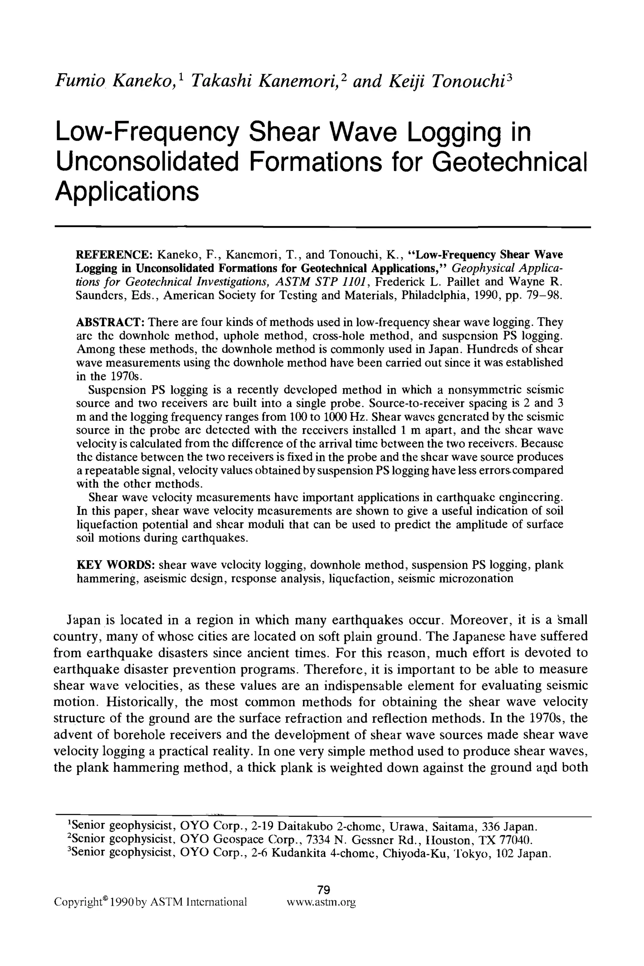
![80 GEOPHYSICALAPPLICATIONS FOR GEOTECHNICAL INVESTIGATIONS
ends are struck by a wooden hammer. This yields very nicely defined shear waves which
can be detected by downhole receivers [1,2].
In recent years, downhole receivers have been developed as an effective method of directly
obtaining shear wave velocity structure. Using these receivers, it is possible to log waves
produced by surface plank hammering down to hundreds of metres. The most recent shear
wave logging method to reach the stage of practical use is suspension logging, which uses
a downhole probe containing both a seismic source and receivers. With suspension logging,
it is possible to measure shear wave velocity down to depths of over 1000 m.
Data obtained by these shear wave velocity logging methods are used in Japan's archi-
tectural engineering and civil engineering fields for aseismic design. The data are also used
in seismic microzonation, which aids in earthquake disaster prevention planning. This paper
covers these shear wave velocity logging methods and their applications.
Shear Wave Velocity Measurement Methods
The methods used for measuring shear wave velocity in situ are downhole shear wave
logging, surface refraction, and reflection methods. Table 1shows the shear logging methods.
These are the downhole, uphole, cross-hole, and the suspension methods. Because compres-
sion wave (P-wave) velocity can also be obtained at the same time, these methods are called
PS logging in Japan. With the exception of the cross-hole method, only one borehole is
necessary in PS logging. The downhole method and the suspension PS logging, which are
used frequently, are described in detail as follows.
Downhole Method
The downhole method is the most common of the PS logging methods. Figure 1 shows a
schematic of the downhole method. A downhole receiver containing three component geo-
phones (two horizontal and one vertical) is firmly clamped to the borehole wall. Surface
plank hammering is commonly used as the shear wave source. Shear wave records shown
in Fig. 2 are obtained at each measuring depth. The upper record is a shear wave record
obtained by striking one side of the plank, and the middle is obtained by striking the other
side. The bottom one is a P-wave record using weight dropping as a seismic source. Com-
paring both shear wave records, polarity is reversed for each other. The property of the
reversed polarity can be used to confirm that it is a shear wave.
Usually, source frequencies are 10 to 50 Hz in unconsolidated soils or sediments. In more
consolidated or partially cemented sediments, the source generates higher frequencies. The
downhole method is normally used at depths of 100 m or less, but useful results can sometimes
be obtained at much greater depths.
Records obtained at each depth are traced up in order of depth. Figure 3 shows the trace-
up records. In the figure, it can be seen that the shear wave propagates downward. Reading
the arrival time of the shear wave at each depth, a travel time curve is made to determine
the velocity layer structure as shown in Fig. 4. Results of the analysis are summarized as
shown in Fig. 5, comparing geological and physical property values. Dynamic elastic coef-
ficients (Poisson's ratio, rigidity factor or shear modulus, Young's modulus, and so forth)
can be calculated from compression and shear wave velocities by using the following equa-
tions [3].
Rigidity factor G = I/52
Young's modulus E = 2(1 + v)G
Poisson's ratio v = [(V/Vs)2/2 - 1]/[(Vp/Vs) 2- 1]](https://image.slidesharecdn.com/geophysicalapplicationsforgeotechnicalinvestigations-151104153926-lva1-app6892/75/Geotechnical-Geophysics-82-2048.jpg)
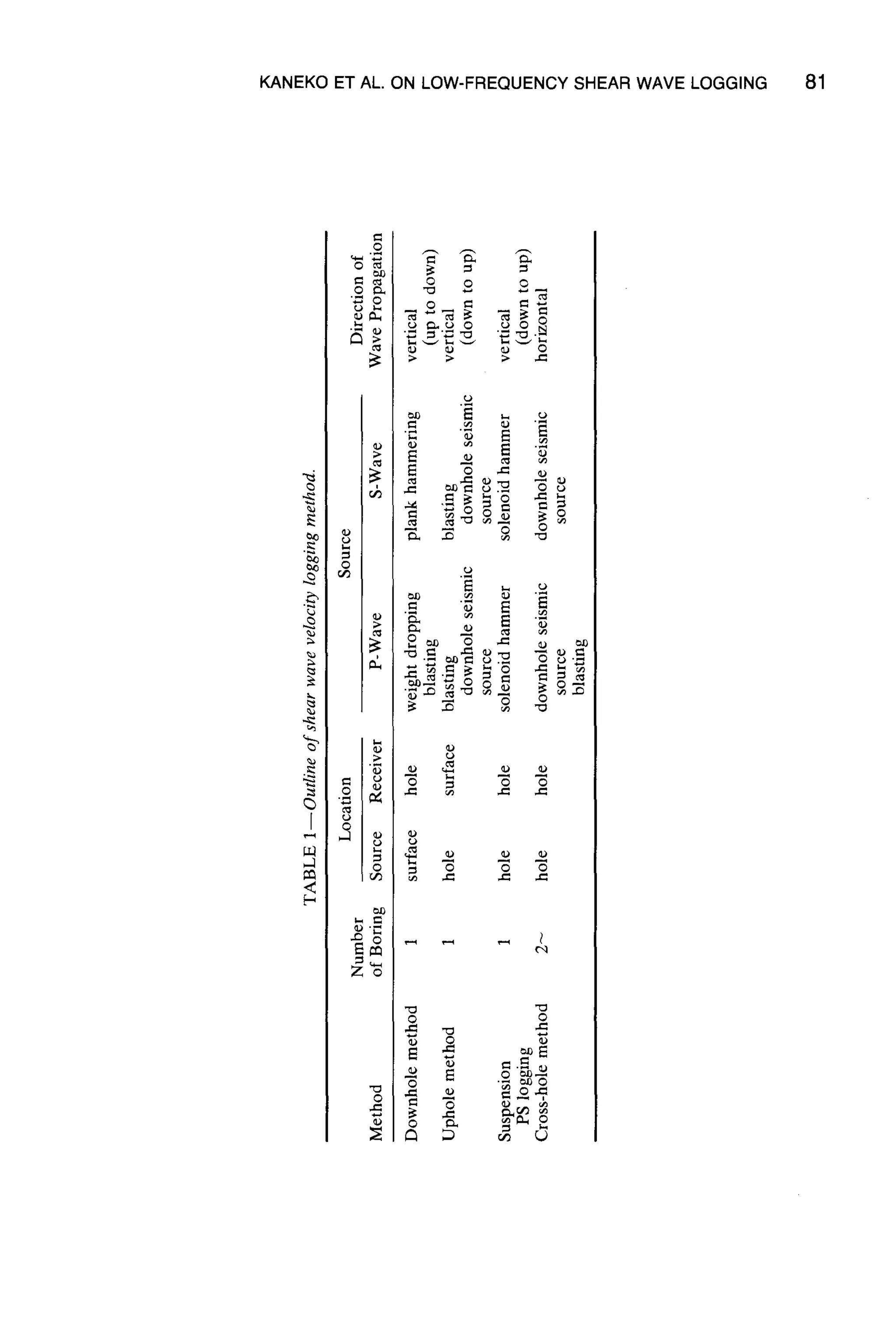
![82 GEOPHYSICAL APPLICATIONS FOR GEOTECHNICAL INVESTIGATIONS
J
Shot mark .~1 I [
_ ~ Amp. ~)~Recorder
P wave shot mark
source S wave
S wave
SOUFCe
A: Weight dropping
B: Striking horizontally
C: Blasting
Receiver
(Borehole pick)
Borehole
FIG. 1--Measuring system of the downholemethod.
where
Vp = compression wave velocity,
V~ = shear wave velocity, and
p = density.
Suspension PS Logging
Suspension PS logging is a recently developed method [4]. Figure 6 shows a schematic of
a suspension PS logging system. A seismic source and two receivers are built in one probe.
Compression and shear waves generated by the seismic source are recorded by the receivers.
Velocity values are calculated from the difference of arrival time between the two receivers.
A solenoid hammer is used as a mechanism of the seismic source. The hammer hits the
borehole wall through the borehole fluid and generates a seismic wave. The hammer can
work back and forth horizontally by changing the polarity of the current flow in a coil. The](https://image.slidesharecdn.com/geophysicalapplicationsforgeotechnicalinvestigations-151104153926-lva1-app6892/75/Geotechnical-Geophysics-84-2048.jpg)
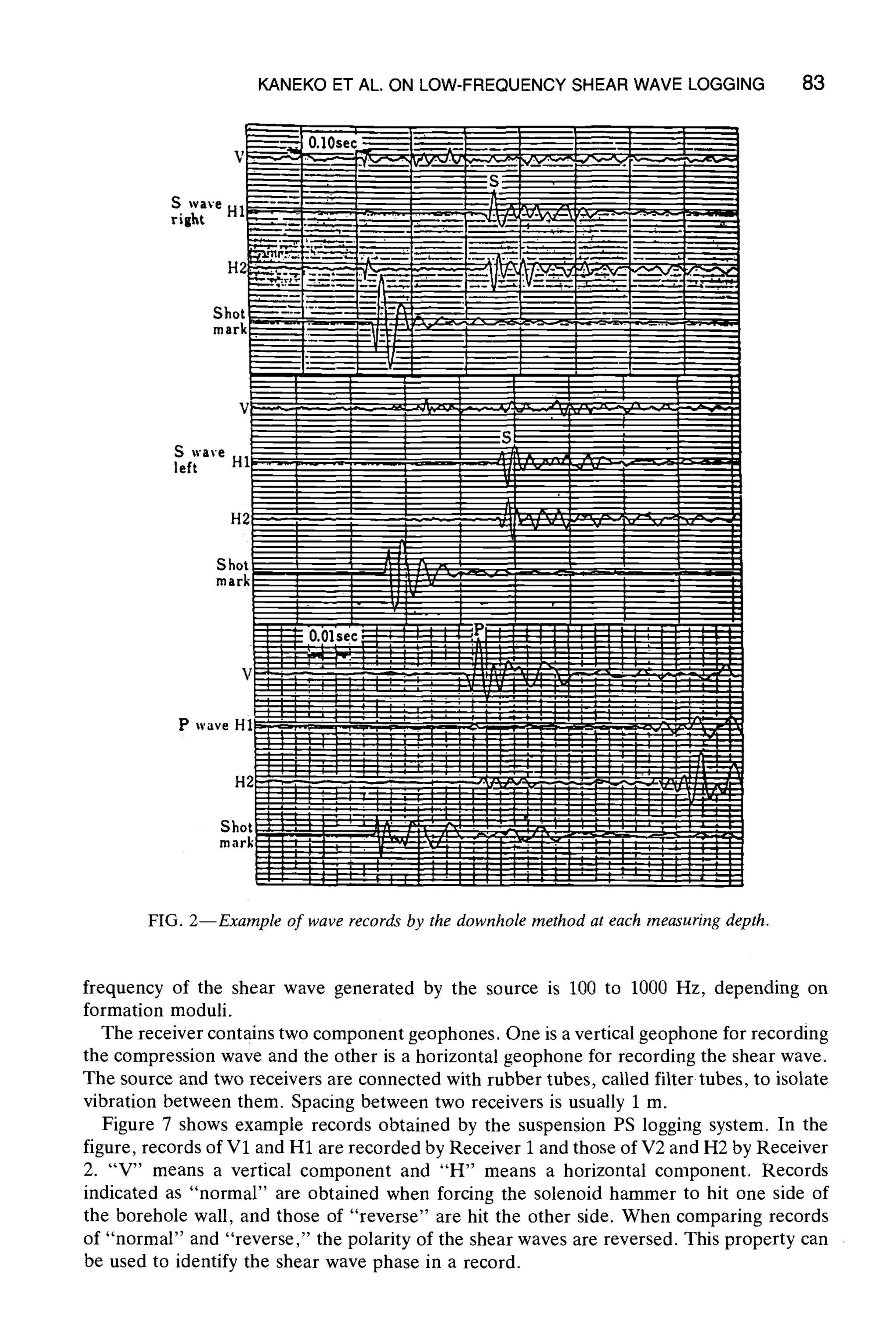
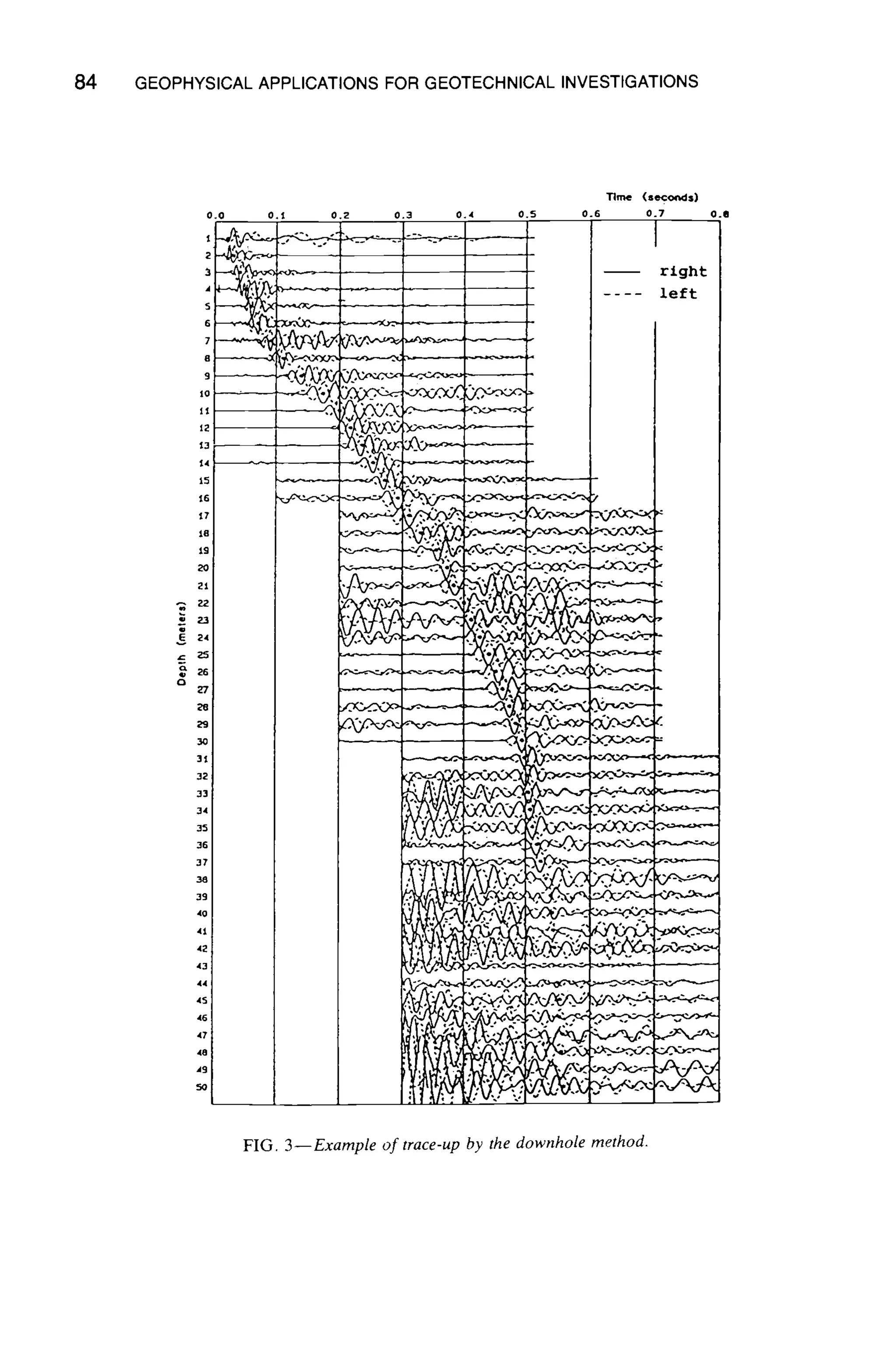
![KANEKO ET AL. ON LOW-FREQUENCYSHEARWAVE LOGGING 85
FIG. 4--Example of travel time curves by the downhole method.
One of the most important features of the suspension PS logging is that it is not necessary
to clamp the probe against the borehole wall. Specific gravity of the probe is around 1.0,
so that the probe behaves in the same way as the borehole fluid. Because the wave length
of excited shear waves is much greater than the borehole diameter, shear excitation is almost
independent of borehole fluid [5,6], or behavior of the borehole fluid is also the same as
the borehole wall. Therefore, geophones in the probe can record the behavior of the borehole
wall without clamping the probe. At the same time, source excitation is highly repeatable
because the source signature does not depend on the efficiency of geophone clamping. The](https://image.slidesharecdn.com/geophysicalapplicationsforgeotechnicalinvestigations-151104153926-lva1-app6892/75/Geotechnical-Geophysics-87-2048.jpg)
![86 GEOPHYSICAL APPLICATIONS FOR GEOTECHNICAL INVESTIGATIONS
a) -c "Ve2~
o r ~ ( g/ ') |
.~_ (In) 10 1ON 0 (re~s) 2000 (kg/cm'l
. .. -.- ~=513.:::.-'~_ Sandy 5 GL ! u,.t.,4)
clay b -3,,
5.o I I c-ls~
5
7.o'----~ Silti~-IGL_6n::(p = l . .qMi)
-- I
GL-8n
~:~
10- ~ t. ~GL-IIm {#-1.231
15- ' =~" 1 ~-0.4)9G- 36
Clay i, ~::loe
~ i .......'
- - 1
20- __ 'I
IGL-21.5m ~
G= 61
~ [. 2O7
25- ! i (~-'-a')
.___--Silt with
:_-_~volcanic G=I/Or_ J
29.0 "vv'4'~ glas~ E=362
30- 31.0 Clay ~ ~1GL- 30m 1o- I. 11@1
.... i v=o.4?e
io G. 16114
.... Silt '~ i t''~9~la
i
Clay '= I t i ,.ez~
39,0 L~CL L_
4 O- "---------:.... i-:9m
I
..... II
45- _---_-~- Silt ).:
I
50-
55-
FIG. 5--Surnrnarized soil column using the downhole method's result.
use of a suspension-type source increases logging speed, making procedures simpler than
with other conventional methods.
The other advantage of suspension PS logging is accuracy of the measured shear velocity
values. Generally, the velocity value is calculated by dividing the propagation path by the
propagation time. In suspension PS logging, spacing between two receivers is fixed me-
chanically in the probe, so there is no error in the propagation path. Also. because the
frequency of the shear wave generated bv the source is higher than the other methods,
wavelengths are shorter and propagation time measurements are more accurate [5, 7]. Fur-
ther, the short measuring interval increases vertical resolution.](https://image.slidesharecdn.com/geophysicalapplicationsforgeotechnicalinvestigations-151104153926-lva1-app6892/75/Geotechnical-Geophysics-88-2048.jpg)
![KANEKO ET AL. ON LOW-FREQUENCYSHEARWAVE LOGGING 87
9~ ~ Winch
(Meter drive)
Pre amp.
P and S
waves
Receiver 1
/
Tube
Source
Driver
for source
Weight
Borehole
FIG. 6--Measuring systemof suspension PS logging.
Shear Wave Velocities in the Ground in Japan
In Japan, the downhole method is most commonly conducted in the disciplines of archi-
tectural engineering and civil engineering. A great volume of data has been accumulated
by this method and has been categorized according to different types of geology. Figure 8
shows the relationship between shear wave velocities and different types of geologic struc-
tures [8]. There is a certain range of values within each type of geology, but the values well
express geological characteristics, and the differences among types of geology are clear.
Figure 9 shows the N value, defined as the number of blows for a 30-era penetration of a
Raymond Sampler driven by dropping a 63.5-kg weight, obtained by standard penetration
tests conducted during drilling investigations. The data is arranged according to type of
geology. Relationships have also been established between shear wave velocity and other
soil constants. When a shear wave velocity measurement cannot be conducted, those re-
lationships with soil properties, such as N value and so forth, are used to estimate shear
wave velocity values.](https://image.slidesharecdn.com/geophysicalapplicationsforgeotechnicalinvestigations-151104153926-lva1-app6892/75/Geotechnical-Geophysics-89-2048.jpg)
![88 GEOPHYSICAL APPLICATIONS FOR GEOTECHNICAL INVESTIGATIONS
Normal -
1t2 ~
Reverse ~.
,'2 ~
Normal
Reverse ~/.:
V1 ~
FIG. 7--Example of wave records by suspension PS logging at each measuring depth.
FIG. 8--Distributions of P- and S-wave velocities (soil type) [8].](https://image.slidesharecdn.com/geophysicalapplicationsforgeotechnicalinvestigations-151104153926-lva1-app6892/75/Geotechnical-Geophysics-90-2048.jpg)
![KANEKO ET AL. ON LOW-FREQUENCY SHEAR WAVE LOGGING 89
FIG. 9--S-wave velocity and N-value (soil type) [8].
N ~uau)
Application
Use of Shear Wave Velocity for Aseismic Design
It is very common to estimate ground behavior during an earthquake and subject it to
response analysis for use in the aseismic design of structures. The methods used for cal-
culation are the wave theory method, the lumped mass method, the finite element method,
and so forth. Figure 10 shows an example of response analysis results according to the wave
theory. In this calculation, shear wave velocity, density, damping factor, and thickness are](https://image.slidesharecdn.com/geophysicalapplicationsforgeotechnicalinvestigations-151104153926-lva1-app6892/75/Geotechnical-Geophysics-91-2048.jpg)
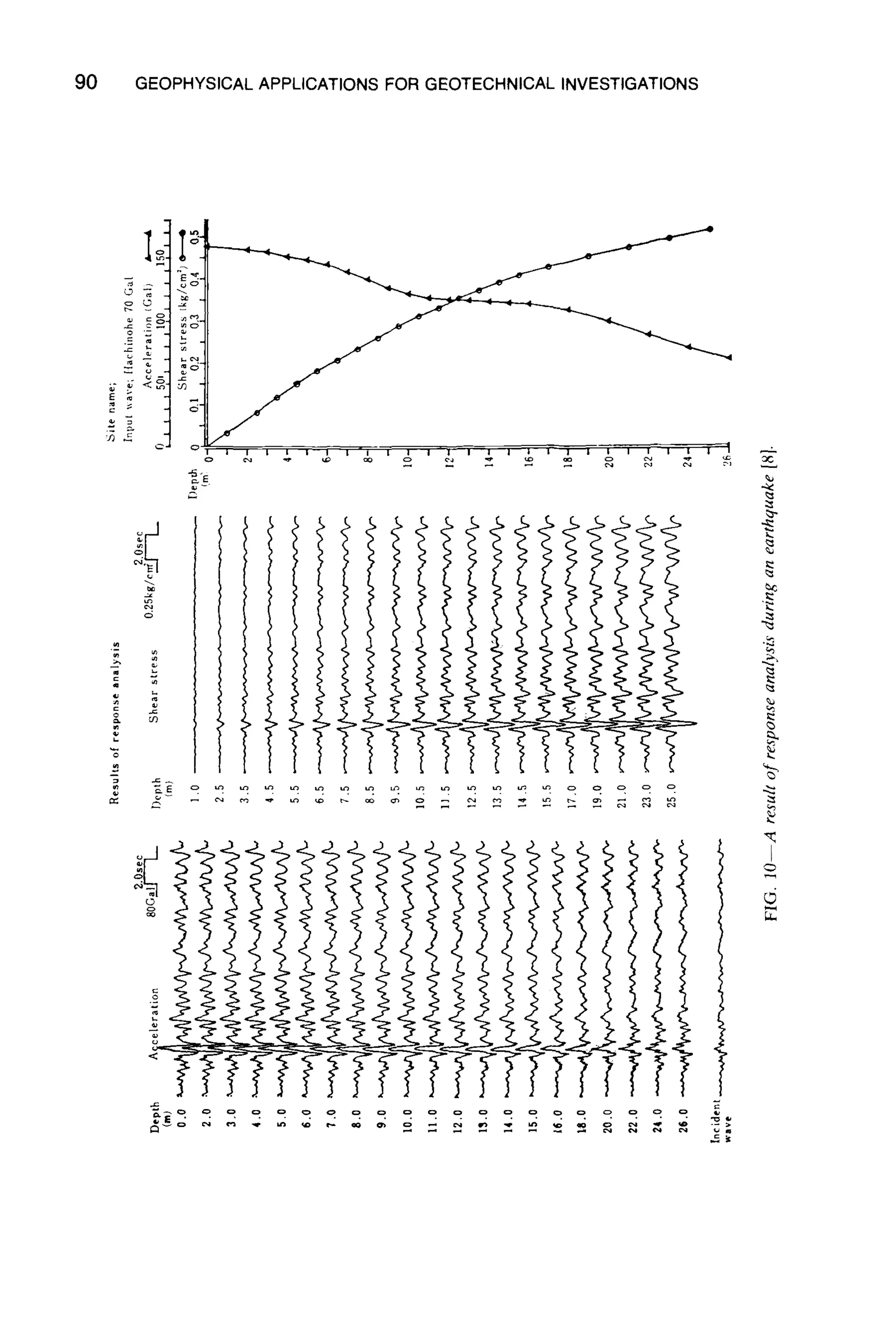
![KANEKO ET AL. ON LOW-FREQUENCY SHEAR WAVE LOGGING 91
assigned to each layer for the case of seismic waves vertically incidental to the base layer.
Response acceleration and shear stress waveforms at each depth are calculated. Thus, shear
wave velocities are one of the most important factors for evaluation of soils in response to
seismic forcing.
Use of Shear Wave Velocity for Liquefaction Evaluation
Liquefaction of sandy ground during an earthquake is one major cause of earthquake
damage. For this reason, evaluation of liquefaction potential, taking seismic force into
account, is conducted in sandy layers. Figure 11 shows the evaluation procedure. Figure 12
is an example of the evaluation of the liquefaction potential of the ground at Showa Ohashi
Bridge, where liquefaction caused major damage during the 1964 Niigata earthquake [9].
In the figure, FL is the liquefaction resistance coefficient. When FL < 1, liquefaction is
considered possible. In evaluating the liquefaction potential, shear wave velocity values in
the ground are indispensable in evaluating the shear strength of soils during an earthquake.
Application to Seismic Microzonation
Earthquakes affect not only structures but also the surrounding area, and thus, forecasting
of expected damage during earthquakes is conducted over wide areas. This is necessary for
countermeasures against earthquake disasters. In recent years, seismic microzonation is often
Dynamicproperties~
of the ground Groundmodelincludingshear
wave velocity
Liquefaction may
not occur
Dynamic shear stress
due to earthquake
Iinc:d;ntW:V:I ....]
tion at base layer]
i
I
I
Seismic response
analysis
Dynamic shear stress
in situ
I
Drillingin situ I
l
I
Undisturbedsand 1
sampling
ICyclic undrained ]
triaxialtest in
laboratory
Dynamicshear LiqUefaction
stress resistance
I I
FIG. ll--Scheme o/liquefaction assessment.
I Correctionof dynamic
triaxial test results
due to in situcondition
Liguefactlo~may
occur](https://image.slidesharecdn.com/geophysicalapplicationsforgeotechnicalinvestigations-151104153926-lva1-app6892/75/Geotechnical-Geophysics-93-2048.jpg)
![92 GEOPHYSICALAPPLICATIONS FOR GEOTECHNICAL INVESTIGATIONS
N-value
5o 30 lO I
~l,: i
9 .,,,......
I> I ,-,,,o, 5o ,o o , 2 :, - " . I , "
1 -:.::~.1 ' i !t . . "'.: . '. --7 .'. 1-
~ . ~ x ~ i ~ i .i.i!i! iilli "~ . ~.', i , .... :'J :':";" """ 9 ::i "' ;ii'i: ~
J-40
FIG. 12--A resultof evaluation ~t liqus ,~otential[9].
conducted to classify soils according to characteristics of seismic motion during an earth-
quake. Large areas are divided into small meshes consisting of squares 500 m on a side,
and response analyses are performed for representative soil types within each mesh. The
distribution of seismic motion during an earthquake is determined in this way.
When calculating seismic motion of the ground surface during an earthquake, source
location, propagation of seismic waves, and the response of the surface layers are important
elements. Since the number of meshes runs to the thousands, it is difficult to obtain shear
velocity measurements to cover the whole area to be mapped. Therefore, geological materials
are collected, and on the basis of a geology descriptions, N values, and so forth, correlated
with measured shear wave velocities and representative locations.
Figure 13 is an example of distribution of seismic motion of the ground surface calculated
as described above for Kanagawa Prefecture, which lies to the south of metropolitan Tokyo
[10]. Figure 14 is an example of evaluation of liquefaction potential [10]. In Kanagawa
prefecture, damage predictions were based on these results, and present anti-earthquake
disaster countermeasures are now being considered.
Use of Shear Wave Velocity in the Evaluation of Seismic Behavior of the Ground During
an Earthquake in Mexico City
During the Michoacan earthquake (Ms = 8.1; surface wave magnitude) of September
1985, there was a great deal of damage in Mexico City, 400 km from the epicenter region.
Mexico City has an extremely soft lake deposit layer underlying it and is surrounded by a
mountainous region. PS loggings were conducted here to determine the reasons for the
cause of damage and formulate an earthquake disaster countermeasure plan. Figures 15 and
16 are a map and profile of Mexico City [11]. As shown in Fig. 17, earthquake observation
has been conducted in Mexico City. The greatest acceleration has been recorded at Point
SCT. Figure 3 is a shear wave velocity measurement record obtained at SCT by the downhole
method [121. Figure 18 is measurement results obtained by the downhole and suspension
methods. In this figure, the cone index, qc, the resistance value during penetration of the](https://image.slidesharecdn.com/geophysicalapplicationsforgeotechnicalinvestigations-151104153926-lva1-app6892/75/Geotechnical-Geophysics-94-2048.jpg)
![KANEKO ET AL. ON LOW-FREQUENCY SHEAR WAVE LOGGING 93
FIG. 13--Estimation of suiJhce acceleration distribution at Kanagawa Pre[i,cture caused by the hy-
pothetical Minami-kanto earthquake [10].
FIG. 14--Evaluation of liquefaction potential distribution at Kanagawa Prefecture caused by the
hypothetical Minami-kanto earthquake [10].](https://image.slidesharecdn.com/geophysicalapplicationsforgeotechnicalinvestigations-151104153926-lva1-app6892/75/Geotechnical-Geophysics-95-2048.jpg)
![94 GEOPHYSICAL APPLICATIONS FOR GEOTECHNICAL INVESTIGATIONS
l lake deposit
transftion zone
volcanic rock
~K~ maln road
z~:7:5 Severelydamaoed areai . . y
4~ ~ by 1985 Michoacan EQ,
(~ StrongMotion Observatory
aF---~ location of profile
(Fig.17)
FIG. 15--Plane of Mexico Basin [11].
0 [0 m FAS
I'~176~-'~-AL- 40 FAI
DP
6o BB
?, t,2, ~,
fill
upper clay formation
hard deposit
lower clay formation
deep deposits
Basalt
FIG. 16--Profile of Mexico Basin [11].
NS NS
QJUNAM ~ (~)Frigorifico
Sitet ~ E W
NS NS
Site2 EW
(structure) ~ ' - "
NS NS
~) ~ ~)Viveros
Site3 EW EW
1} 20 40 60 (sec) 0 20 40 60(sec)
1200g~l
NS
(~)Oficina
NS
(~Tacabaya ---~ ~-~'~A~"-----~
EW
0 20 40 r~ 80 I00 ;2~ 140 160(see)
FIG. 17--Observed accelerograms at Mexico City [l 1].](https://image.slidesharecdn.com/geophysicalapplicationsforgeotechnicalinvestigations-151104153926-lva1-app6892/75/Geotechnical-Geophysics-96-2048.jpg)
![KANEKO ET AL. ON LOW-FREQUENCYSHEARWAVE LOGGING 95
38
Q
35
48
45
58
g5
I
28i
v8 vp
downhole
qc - -
5usperlslon ~ + +
Uolocit~ (m/~oc)
58 188 288 588 1888 2888
J P-wave
s .... e -~
L~
28 '~~
)-
i I i i i , I i i i i i i
qc (k9/r
]*
12
1.
9l ~
I:
L
I'
)
['.
[~
I ~
I"
89
r.
*l ~
,J"
I
I
I
I
I
z~e
FIG. 18--Resuh of PS logging at SCT.
cone penetrometer, is also given, Cone index qc shows a very good correlation with shear
wave velocity Vs. Compared to the results from the downhole method, the results from the
suspension method give a greatly detailed velocity structure,
As these figures show, at the depth range of 6 to 30 m, the ground consists of a very soft
clay deposit having shear wave velocity values of less than 100 m/s and including values as
low as 33 mJs. Soft layers like these amplify seismic motion and are thought to have greatly
contributed to the damage to buildings.
To confirm this, observed waveforms obtained at SCT were compared with waveforms
obtained by response analysis. Table 2 shows a ground model and Fig. 19 shows a simplified
profile model. Figure 20 shows calculation results. 'First, vertical incidental seismic waves
from the bottom were calculated by the wave theory using observed waves at a rock site.
This is result b. This well accounts for the first half of the observed waveform on the soft
ground (e). But in the latter half, a difference can be seen. Since this can be thought to be
due to soft layers near SCT, the ray-tracing method [13] was used to calculate seismic motion
propagated in surface layers from the edge of the basin (c) (see Fig. 19). The result (c) was
superimposed on the seismic wave directly and vertically incidental from the bottom (b).](https://image.slidesharecdn.com/geophysicalapplicationsforgeotechnicalinvestigations-151104153926-lva1-app6892/75/Geotechnical-Geophysics-97-2048.jpg)
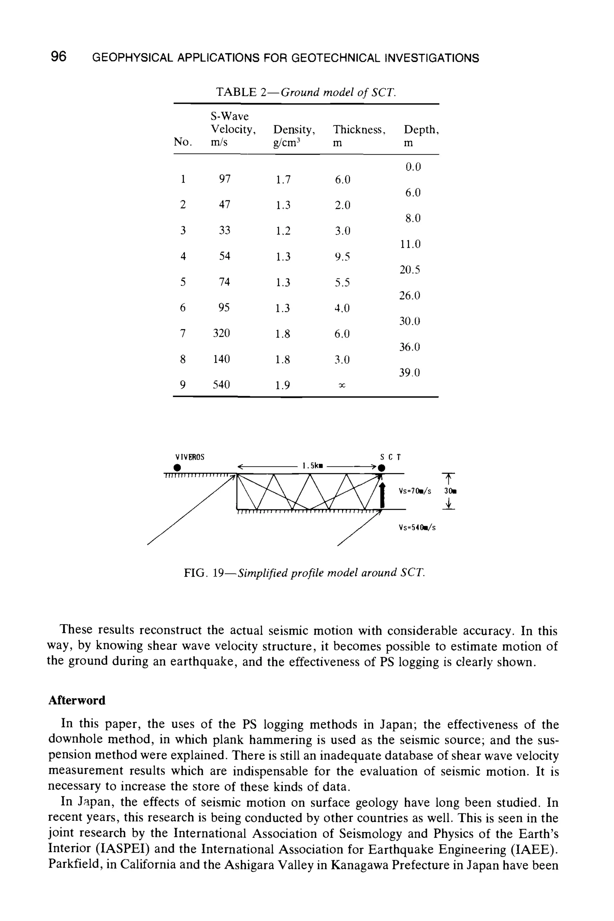
![KANEKO ET AL. ON LOW-FREQUENCY SHEAR WAVE LOGGING 97
(GhL)
{a] oDserved : Vlveros EW
CO0.O-
4Z'~'20
i
-COO,O-
I
0.0 40,0 80,0 120,0
]
160,0
($EC)
({;AL)
COQ.0~
.27
[b] estlmated : vertical multi
103,1
; - - v v , y ~ V V v V ~ V ~ v w . . . . . . .
200,0~
[C] ~stlmated : horizontally multl
V-
-I~IoS
I
0.0 40,0 80,0 IL~O,O 160.0
SEC
(GAL) [d] estimated : It)] + Cc]
200*0/~ J ] 9
-162.4
(GAL) ~] observed ~n~ should be Comnated : SET EW
167.S
I----"- I ~ - - I T I ~ 1 ~ I "l
0.0 40.0 80,0 120.0 lg0.0
(SEC}
FIG. 20--Results of response analysis at SCT.
designated as test sites for investigations and earthquake observation now being conducted.
At present, the stage of considering various forecasting methods has been reached. Hope-
fully, these methods will be carried out on a worldwide scale and they will serve to identify
dynamic characteristics of the ground and promote earthquake disaster planning.
References
[I] Uchiyama, S.,"P and S-Wave Velocity Measurement Using Boreholes," Butsurimnko, Vol. 36,
No. 5, 1983 (in Japanese).
[2] Uchiyama, S., Tonouchi, K., and Imai, T., "Measurement of S-Wave Velocity of the Ground and
Application of S-Wave Velocity Data for Civil Engineering," OYO TechnicalNote, No. 52, 1984.
[3] White, J. E., UndergroundSound-Applications of Seismic Waves, Elsevier, New York, 1983.](https://image.slidesharecdn.com/geophysicalapplicationsforgeotechnicalinvestigations-151104153926-lva1-app6892/75/Geotechnical-Geophysics-99-2048.jpg)
![98 GEOPHYSICAL APPLICATIONS FOR GEOTECHNICAL INVESTIGATIONS
[4] Kitsunezaki, C., "A New Method for Shear Wave Logging," Geophysics, Vol. 45. 1980.
[5] Chen, S. T., "Shear-Wave Logging with Dipole Sources," Geophysics, Vol. 53, 1988.
[6] Schmitt, D. P., "Shear Wave Logging in Elastic Formations," Journal of the Acoustical Societv
of America, Vol. 84, 1988.
[7] Chert, S. T. and Willen, D. E., "Shear Wave Logging in a Slow Formation," paper presented at
the Society of Professional Well Log Analysis 25th Annual Logging Symposium, New Orleans,
1984.
[8] Imai, T. and Tonouchi, K., "Correlation of N-Value with S-Wave Velocity and Shear Modulus,"
in Proceedings of the 2nd European Symposium on Penetration Testing, 1982.
[9] Iwasaki, T. and Tokita, K., "The Earthquake Proof Investigation of the Ground at Showa-Ohashi
Bridge, Niigata City." presented at the 15th Japan National Conference on Soil Mechanics and
Foundation Engineering, 1980 (in Japanese).
[10] "Report of Earthquake Countermeasures in Kanagawa Prefecture." Kanagawa Prefecture. 1985
(in Japanese).
[11] "Report on Survey of Damage Caused by the September 19. 1985 Mexico (Michoacan) Earth-
quake," OYO Corp., Hirata Structural Engineers Co.. 1986 (in Japanese ~ith abstract in English).
[12] Jaime, A. and Romo, M. P., "The Mexico Earthquake of September 19, 1985--Correlations
Between Dynamic and Static Properties of Mexico City Clay.'" Earthquake Spectra. Vol. 4, No.
4, 1988.
[13] Seo, K., "Interpretation of Strong Motion Accelerographs Based on Underground Structure."
presented at the 14th Symposium on Seismic Ground Motion. A.I.J.. 1986 (in Japanese).](https://image.slidesharecdn.com/geophysicalapplicationsforgeotechnicalinvestigations-151104153926-lva1-app6892/75/Geotechnical-Geophysics-100-2048.jpg)
![Alfred E. Hess1 and Frederick L. Paillet'
Applications of the Thermal-Pulse
Flowmeter in the Hydraulic Characterization
of Fractured Rocks
REFERENCE: Hess, A. E. and Paillet, F. L., "Applications of the Thermal-Pulse Flowmeter
in the Hydraulic Characterization of Fractured Rocks," Geophysical Applications for Geo-
technical Investigations, ASTM STP 1101, Frederick L. Paillet and Wayne R. Saunders, Eds.,
American Society for Testing and Materials, Philadelphia, 1990, pp. 99-112.
ABSTRACT: The U.S. Geological Survey has developed a thermal-pulse flowmeter capable
of detecting borehole flows to as small as 0.04 L/min. This new flowmeter provides much
greater sensitivity to slow vertical flow than that available using conventional spinner flow-
meters. This paper describes five applications of the thermal-pulse flowmeter in the charac-
terization of the hydrology of fractured rocks. These applications include measurement of
flows in boreholes driven by ambient hydraulic-head differences, identification of fractures
contributingflow during production tests, inference of fracture interconnections during aquifer
tests, interpretation of water-quality contrasts in boreholes, and identification of fractures
affected by hydraulic stimulation procedures. Each of the five applications is illustrated by
specific examples selected from ongoing research activities at various fracture hydrologystudy
sites.
KEY WORDS: boreholes, fracture flow, logging, hydrology, thermal-pulse flowmeter
Flowmeter logging is recognized as an effective method for the identification of formations
or fracture zones that produce water during aquifer tests [1,2]. In some situations, the vertical
profile of discharge obtained by using conventional spinner flowmeters can be analyzed to
determine the vertical distribution of permeability adjacent to the borehole [3]. However,
conventional spinner flowmeters cannot be used to measure discharges in boreholes that
produce water from relatively impermeable formations because such formations do not
produce enough flow to turn the blades or vanes of the spinner. Alternative borehole flow-
sensing equipment capable of detecting very small borehole discharges may have useful
applications in the characterization of fracture permeability distributions in low-permeability
fractured formations.
The U.S. Geological Survey has developed a thermal-pulse (TP) flowmeter capable of
measuring borehole discharges as small as 0.04 L/min. This paper describes some of the
applications that have been found for the TP flowmeter in the hydraulic characterization of
fractured rocks. We present brief examples of flowmeter applications at five different field
sites. These examples illustrate applications including: (1) measurement of flows in boreholes
driven by ambient hydraulic-head differences between separate fracture zones, (2) identi-
fication of individual fractures that produce flow during production tests, (3) fracture in-
1Electronic engineer and project chief, respectively, U.S. Geological Survey, Box 25046, MS 403,
Denver Federal Center, Denver, CO 80225-0046.
99
Copyright91990by ASTMlntcrnational www.astm.org](https://image.slidesharecdn.com/geophysicalapplicationsforgeotechnicalinvestigations-151104153926-lva1-app6892/75/Geotechnical-Geophysics-101-2048.jpg)
![100 GEOPHYSICALAPPLICATIONSFOR GEOTECHNICALINVESTIGATIONS
terconnections indicated by flowmeter measurements obtained during cross-hole pumping
tests, (4) interpretation of water-quality contrasts in boreholes, and (5) identification of
fractures affected by hydraulic fracture stimulation. Each of these examples represents
hydrologic information that could not have been obtained by using conventional spinner
flowmeters, and each has made a significant contribution to an ongoing study of fractured
rock hydrology.
Thermal.Pulse Flowmeter
The need for a flowmeter with slow-velocity sensitivity prompted the U.S. Geological
Survey to develop a small-diameter TP flowmeter that would operate to depths of 3000 m
or more through 5000 m or longer lengths of conventional four-conductor logging cable
(Fig. 1). The TP flowmeter that was developed by the U.S. Geological Survey has inter-
changeable flow sensors, 41 and 64 mm in diameter, and slow-flow sensitivity from 0.04 to
6.1 m/rain in boreholes with diameters that range from 50 to 125 mm. The vertical velocity
of the water in a borehole is measured with the TP flowmeter by measuring the time between
the trigger pulse and the response peak of a relative-temperature sensor (Fig. 2) and de-
termining the velocity (or volume flow) from calibration charts that were developed in the
laboratory using tubes with diameters similar to those of the boreholes under investigation
[4].
After the TP flowmeter was tested at several sites, the U.S. Geological Survey determined
that there was a need for, and subsequently developed, a wireline-powered, inflatable, flow-
concentrating packer [5]. The packer decreases the measurement uncertainties caused by
geothermally induced convection currents within the borehole [6] and increases flow sen-
sitivity in larger diameter holes. The TP flowmeter and packer have been integrated into a
single probe that operates on logging lines with four or more electrical conductors (Fig. 3).
The packer system requires only a single conductor (plus the cable armor). The packer
system also may be used with other borehole probes, such as spinner flowmeters and pressure
transducers, whose function would be enhanced with the use of an easily inflatable packer.
The TP flowmeter, with and without the packer, has been used to measure natural and
artificially induced flow distributions in boreholes with diameters ranging from 75 to 250
mm, at temperatures from 6 to 60~ and in a variety of lithologies including basalt, dolomite,
gneiss, granite, limestone, sandstone, and shale. When the inflated packer is used to direct
all borehole flow through the flow-sensor section, the measured thermal travel times correlate
with borehole discharge, rather than average vertical velocity. When the packer is inflated,
the TP flowmeter measures borehole flows in the range of 0.04 to 8 L/rain. A representative
flow-calibration chart for the thermal flowmeter, with separate curves for operation when
the flow-concentrating packer is inflated, deflated, or absent, is shown in Fig, 4. The inverse
of the travel time is used in the calibration chart to simplify the plotting and reading of the
calibration curves [6].
The TP flowmeter initially was used to define flows in boreholes occurring under ambient
conditions. However, additional applications have been determined for the TP flowmeter,
such as locating fractures that produce water during aquifer tests and identifying flows
induced in adjacent boreholes during such tests. The capability of rapid measurement of
slow flow provided by the TP flowmeter means that a few hours of flow measurements have
the potential for saving many days of investigation using conventional hydraulic testing and
tracer techniques.](https://image.slidesharecdn.com/geophysicalapplicationsforgeotechnicalinvestigations-151104153926-lva1-app6892/75/Geotechnical-Geophysics-102-2048.jpg)
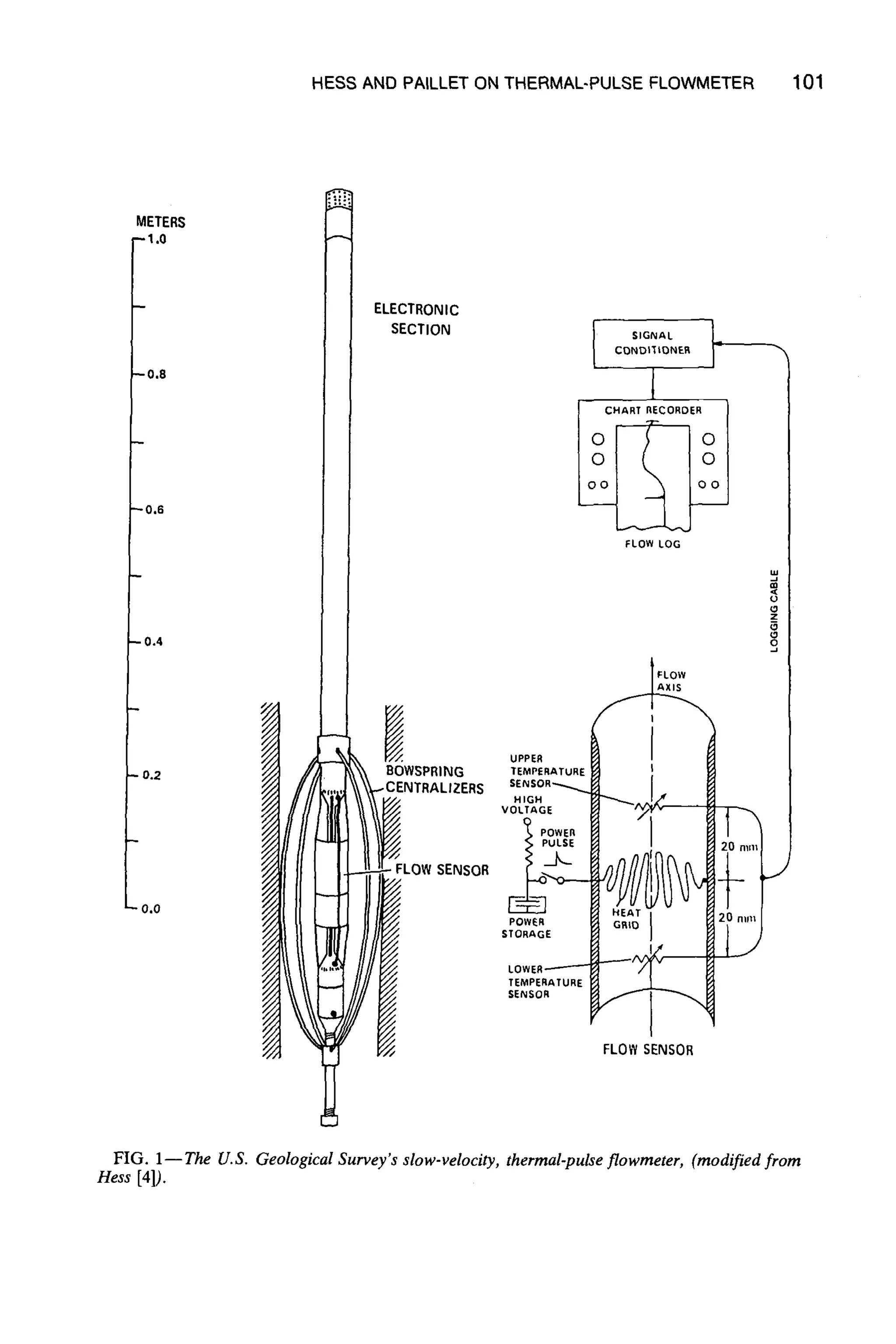
![102 GEOPHYSICALAPPLICATIONSFOR GEOTECHNICALINVESTIGATIONS
A 13
V-
TRIGGER UPFLOW RESPONSE PEAK
PULSE I
0LSETR L,,ME
1 I [ I
L ,~, d
"f~IGGER
PULSE
1
I
DOWNFLOW RESPONSE PEAK
PULSE 3T~AVELTIME ~!
I I I
FIG. 2--Typical thermal-pulseflowmeter output responses."(a) upflow responseand (b) downflow
response (modifiedfrom Hess [4]).
Flowmeter Applications
Measurement of Ambient Flow in Boreholes
Fractures provide discrete pathways for fluid flow in otherwise nearly impermeable for-
mations. The relative isolation of permeable fracture conduits within the rock mass can
enable natural hydraulic-head differences between different sets of fractures to develop.
When a borehole intersects two or more such isolated or poorly connected fracture flow
systems, the existing hydraulic-head differences cause fluid to flow through the borehole
between the fractures. In other situations, regional drawdowns produced by pumping from
fractured aquifers are propagated to different radii in different fracture zones, which produce
measurable hydraulic-head differences in which separate fracture zones are intersected by
a single observation borehole. In either of these situations, the measurement of flows driven
by the ambient head differences and the properties of the fractures in which fluid enters or
exits the borehole can provide useful information about fracture hydraulics.
An example of the type of information that one can obtain from the identification of
convection flow under ambient conditions in boreholes is illustrated in Fig. 5. These vertical
flow measurements illustrate the natural convection in a borehole drilled into the gabbroic
rocks of a small upland area near the southern limit of the Canadian Shield in central
Ontario. The distribution of fractures indicated by core observations demonstrates that a
number of apparently permeable fractures and fracture zones intersect the borehole. Fluid
enters the borehole at several of the shallow fractures and exits at a single large fracture
zone near the bottom of the borehole. Subsequent study at this site indicated that the deep
fracture zone is one of several regional fracture zones located near the base of the gabbroic
rock mass. Shallow fractures apparently had been recharged by recent rainfall, while the
deep fracture zone was still characterized by decreased hydraulic heads associated with an
earlier period of drought and discharged into topographically low areas along the periphery
of the upland. Information about the naturally occurring hydraulic-head differences between
shallow and deep fracture zones such as that shown in Fig. 5 was helpful in describing the
fracture flow systems involved in ground-water circulation through this gabbroic rock
mass [7].
Production Tests in Tight Formations
The relatively small discharges produced by the drawdown in boreholes penetrating low-
permeability formations made it nearly impossible to use conventional spinner flowmeter](https://image.slidesharecdn.com/geophysicalapplicationsforgeotechnicalinvestigations-151104153926-lva1-app6892/75/Geotechnical-Geophysics-104-2048.jpg)
![:~ONIC
"ION
HESS AND PAILLET ON THERMAL-PULSE FLOWMETER 103
METERS
-1.0
--0,8
0.6
0.4
FLOWSENSORWITH
INFLATEDPACKER
0.2
o.o
VALVE
BOX
FIG. 3 -- The U,S. Geological Survey's thermal-pulse flowmeter with inflatedflow-concentrating packer
(modified from Hess [5]).](https://image.slidesharecdn.com/geophysicalapplicationsforgeotechnicalinvestigations-151104153926-lva1-app6892/75/Geotechnical-Geophysics-105-2048.jpg)
![104 GEOPHYSICAL APPLICATIONS FOR GEOTECHNICAL INVESTIGATIONS
z
z*
g
EXAMPLE OF A TP-ELOWMETER CALIBRATION
IN A 152 mm DJA, COLUMN
1.0 u =
0,8
// i,~~ # , ~
o. // ,8
" // .. s'" 9 z
-0,2 ,...- ;]I 4
.0,4 ...... ,/~' '._8 ~o
-o,o- /1 t .-I:, o
-0.8 . /I/"_ 1
,O,o o8 o'o DO o, o~
INVERSE RESPONSE TIME, IN 1/SEC
-- NO PACKER --~ DEFLATED PAC .... INFLATED PAC
FIG. 4--Example of a thermal-pulse flowmeter calibration m a 152-ram-diameter calibration column
(modified from Hess and Paillet [14]).
10c
<
~, 20c
o
~- 30Ci.u
z
I
40C
50(
i i k I
9 9 go 9
DOWN FLOW, IN MILLILITERS PER MINUTE
i
1000 5 10
NUMBER OF OPEN
FRACTURES PER
METER OF DEPTH
FIG, 5--Distribution of natural vertical flow in a borehole penetrating .t)'actured gabbroic rocks on
the Canadian Shield in central Ontario compared to the distribution of open fractures identified in core
samples (modified from Paillet and Hess [7]).](https://image.slidesharecdn.com/geophysicalapplicationsforgeotechnicalinvestigations-151104153926-lva1-app6892/75/Geotechnical-Geophysics-106-2048.jpg)
![HESS AND PAILLETON THERMAL-PULSEFLOWMETER 105
measurements to determine depths at which water flowed into the borehole. The improved
sensitivity and resolution of the TP flowmeter enables identification of the individual frac-
tures or sets of fractures producing inflow during simple drawdown or aquifer tests using
low-capacity pumps in tight formations.
An example of the application of the TP flowmeter to the identification of inflow fractures
and borehole productivity is illustrated in Fig. 6. A series of five boreholes was drilled along
a 2000-m profile in the White Mountains of New Hampshire (Fig. 6a). Although all five of
the boreholes intersected numerous fractures (Fig. 6c), well yield estimated from aquifer
tests varied greatly between the boreholes (Fig. 6b). Furthermore, flowmeter measurements
indicated that the inflow to each of the boreholes occurred through a limited number of
individual fractures. These results indicate that only a few of the apparently permeable
fractures intersected by these boreholes produced flow during drawdown. Of special interest
was that in the three boreholes in which more than 10 L/min were produced during drawdown
tests, all the flow came from a single set of fractures intersected in the depth interval from
25 to 45 m. This information is needed by hydrologists attempting to develop models for
the circulation of ground water in fractures beneath the studied lake basin [8,9].
Cross-Hole Pumping Tests
Numerous studies of the hydrology of fractured rocks have indicated that regional flow
occurs by means of transmissive zones, many of which correspond to faults or shear zones
[10-12]. The physical factors that control the rate of flow within these zones and the identity
of the individual fracture segments conducting flow within the zone are of special interest
to the hydrologist. Borehole flow measurements in the pumped borehole and adjacent
observation boreholes can provide important information about the interconnectivity of
fractures within the fracture zones intersecting the boreholes.
Examples of the value of TP flowmeter measurements during cross-borehole pumping
tests in southeastern Manitoba are illustrated in Figs. 7 and 8. The distribution of fracture
permeability in the region of two boreholes (URL-14 and URL-15) was estimated from
interpretation of acoustic-televiewer and acoustic-waveform logs [13]. These logs were an-
alyzed by comparing log data with the calculated response of various fracture models, giving
a qualitative estimate of fracture permeability in terms of the aperture of an equivalent
plane fracture (Fig. 7). The profiles of relative transmissivity in these two boreholes indicate
that permeability is concentrated in a single fracture zone that intersects both boreholes.
However, a number of permeable fractures that do not project between the two boreholes
also occur a few metres above and below the major fracture zone. The two boreholes are
approximately 130 m apart. Individual borehole production tests indicated that Borehole
URL-15 produced 19 L/min from the major fracture zone with 1.5 m of drawdown, while
Borehole URL-14 produced only 0.25 L/min with 80 m of drawdown.
The results of a cross-borehole pumping and flow measurement for this pair of boreholes
are illustrated in Fig. 8. The pattern of fracture interconnection in and adjacent to the major
permeability zone is indicated by the pattern of vertical flow induced in Borehole URL-15
by a drawdown in Borehole URL-14. The near equality of the induced downflow in URL-
15 with the production from Borehole URL-14 (about 0.25 L/rain) indicates that the only
connection between the two boreholes occurs by means of secondary fractures that splay
off of the main fracture zone. The conduction of all cross-borehole flow by fractures splaying
off the main fracture zone was an entirely unexpected result and one with important con-
sequences for the modeling of ground-water circulation at this site where major fracture
zones are assumed to provide the primary subsurface flow pathways.](https://image.slidesharecdn.com/geophysicalapplicationsforgeotechnicalinvestigations-151104153926-lva1-app6892/75/Geotechnical-Geophysics-107-2048.jpg)
![106 GEOPHYSICAL APPLICATIONS FOR GEOTECHNICAL INVESTIGATIONS
~" 3O0 a b
uJ e
A ~ 200 .... t,,,
~oo
,~ o I I
~ a b c d
Om~ 0 200 aO0 600 8~:~ 1000 1200 1400 1600 1800
DISTM'~E ~N METERS
F
/
Y
f, .,,
L__ ~ j,,"-
NEW HAMPSHIRE
a b c d e
NUMBER OF FRACTLRES It,, ~ t,~ETE~ CP BOaERO_E
9 /
)
60- ~
J
o4
1:
I
;ID i84
i r
I
J ~
tl Denotes depth
where one or
~-S ~ more fractures
producing less
~ than 10 liters
per minute
i "Jr Denotes fracture
i or fractures
producing 10 or
i more liters per
~ mlnu(e
i
i i,
4 84
I
, i, 9 i'
FIG. 6--Example of distribution of yields .for adjacent bedrock wells in the White Mountain~ of New
Hampshire: (a) depth and separation of five wells along a 2000-m profile, (b) well yield determined 1"rein
pumping tests, and (c) distribution of permeable fractures idenIified from televiewer logs (modified from
Paillet et al. [15]).](https://image.slidesharecdn.com/geophysicalapplicationsforgeotechnicalinvestigations-151104153926-lva1-app6892/75/Geotechnical-Geophysics-108-2048.jpg)
![HESS AND PAILLET ON THERMAL-PULSE FLOWMETER 107
BOREHOLE BOREHOLE
URL15 URL14
---- '230
240
25O
FRACTURE
........ ZONE ....... ]260 ~=
I,.
I I
0.0 0.2 0.4
270 0
u./
280 ~;
Z
29O
300
I
310
mmm
o.o ol.2 0,4 320
ESTIMATED FRACTURE
APERTURE, IN
MILLIMETERS
FIG. 7--Distribution of estimatedfracture aperture in Boreholes URL14 and URL15 in southeastern
Manitoba deterrninedfrorn acoustic-waveform and othergeophysical logs (modified from Hess and Paillet
[14]).
Water-Quality Applications
Various geophysical logs and fluid samples can be used to indicate the solute content of
water in boreholes. However, the presence of water of a given quality at a certain depth in
a borehole does not always indicate that similar water is present in the formation at that
depth. High-resolution flowmeter logs can be used to determine the location of fractures
or beds producing the water sampled in the borehole.
An example of the application of flowmeter logs in the interpretation of water quality in
situ is illustrated in Fig. 9. A borehole drilled in fractured dolomite in northeastern Illinois
was logged with acoustic televiewer, caliper, single-point resistance, and flowmeter probes.
The caliper and televiewer logs indicated the location of numerous fractures and other
openings intersecting the borehole. The resistance log indicated two abrupt changes in](https://image.slidesharecdn.com/geophysicalapplicationsforgeotechnicalinvestigations-151104153926-lva1-app6892/75/Geotechnical-Geophysics-109-2048.jpg)
![108 GEOPHYSICAL APPLICATIONS FOR GEOTECHNICAL INVESTIGATIONS
URL15 URL14
025 LJmm
PROJECTIONS
OUTFLOW ~.
0 25 IJrnin
/
INFLOW
;.EC.
C~
m
C
t.
3C3
_z
350
FIG. 8--Distribution of vertical flow measured in Boreholes URL14 and URL15 in southeastern
Manitoba that was induced by pumping from URL14. Fracture planes were identified with an acoustic
televiewer (modified from Hess and Paillet [14]).
ACOUSTIC CALIPERLOG RELATIVESINGLE-POrNT FLOWtl,4ETERLOG
TELEVI~E~ LOG RESISTANCELOG
==
w
za 40
5
o~
_z 5O
(3
I I
T5 25
DIAMETERIN CENT}METERS
INCREASING
F~ES STANCE I~
"1
/(
[ i , ~ i i
INFLO% --
40
I
5O
OUTFLOW
60
230 2~0 // 015 00
DOWNFLOW.INLITERS
PERMINUTE
FIG. 9--Acoustic-televiewer, caliper, single-point-resistance, and flowmeter logs from a borehole in
northeastern Illinois (modified from Hess and Paillet [14]).](https://image.slidesharecdn.com/geophysicalapplicationsforgeotechnicalinvestigations-151104153926-lva1-app6892/75/Geotechnical-Geophysics-110-2048.jpg)
![HESS AND PAILLETON THERMAL-PULSEFLOWMETER 109
average resistivity (at about 38 and 54 m in depth) which were interpreted as changes in
the solute content of water in the borehole. However, the fractures or fracture sets producing
these different quality waters could not be determined from these logs alone. The flowmeter
log provided the information required to identify the sources of the different solute contents
in the borehole. The ambient flow consisted of relatively fresh water entering through the
shallow fracture zone (A) just below the bottom of casing, and most of that water exited
at a major fracture at about 33 m in depth (B). A small portion of water from (A) continued
downhole to another large fracture near 38 m in depth (C), where additional water entered
the borehole. This incoming water that has greater solute content mixed with the downflow
from above and produced an intermediate resistivity value on the electric log. All of this
downflow then exited at a fracture near 54 m in depth (D). Below this depth, the single-
point resistance log indicated a further increase in borehole-fluid solute content. The elec-
trical conductivity of this deep water may represent the properties of ground water entering
the borehole at fracture (C) before dilution with the downflow from above. Hess and Paillet
[14]indicate that this pattern of fluid mixing from different depths within the dolomite would
have been nearly impossible to interpret without the flowmeter data.
Identification of FracturesAffected by Hydraulic Fracture Stimulation
Numerous small-capacity water supplies developed for single-family or livestock use rely
upon wells produced from transmissive fractures within otherwise nearly impermeable crys-
talline rocks. In many situations the fractures intersecting the borehole do not produce
adequate water. Hydraulic stimulation of fractures [15]can substantially increase the water
production from most of these boreholes [16,17].
An example of the application of the TP flowmeter in the evaluation of hydraulic fracture
stimulation of water production from a crystalline rock borehole is illustrated in Figs. 10
and 11. The distribution of fractures in a borehole that initially produced less than
0.5 L/min is illustrated in Fig. 10. This well then was stimulated by increasing the hydraulic
pressure below a single packer until the response of a borehole pressure transducer indicated
the opening or inflation of one or more fractures. The procedure was repeated with the
packer set at five increasing depths ranging from 12 to 107 m. The distribution of vertical
flow during constant hydraulic-head recharge before and after hydraulic fracture stimulation
is illustrated in Fig. 11. Before stimulation, most of the recharge was accepted by four
relatively minor fractures (B, C, F, and G in Fig. 10) and by a large fracture (A) located
just above the initial water level. The two very large fractures intersecting the borehole near
45 and 80 m in depth (D and E in Fig. 10) did not accept any of the flow and otherwise
seemed to be completely nonproductive.
After hydraulic fracture stimulation, two of the previously productive fractures, B and
G, accepted about ten times as much flow under the same recharge hydraulic head. The
water level was permanently raised by about 20 cm, which saturated the large fracture (A)
that had been above initial water level and had previously accepted most of the recharge
during the prestimulation flow test. The water level change may have been caused by changes
in the hydraulic conditions in the stimulated fractures or by the saturation of fracture (A)
by the injection of fluid during hydraulic stimulation. The saturation of fracture (A) appears
to account for the large decrease in the volume of flow accepted by that fracture after
stimulation. The increase in production associated with the two fractures at B and G in Fig.
10, seem to account for all of the poststimulation increase in the ground-water production
from 0.5 to 2 L/min that was subsequently measured by the well owner.](https://image.slidesharecdn.com/geophysicalapplicationsforgeotechnicalinvestigations-151104153926-lva1-app6892/75/Geotechnical-Geophysics-111-2048.jpg)
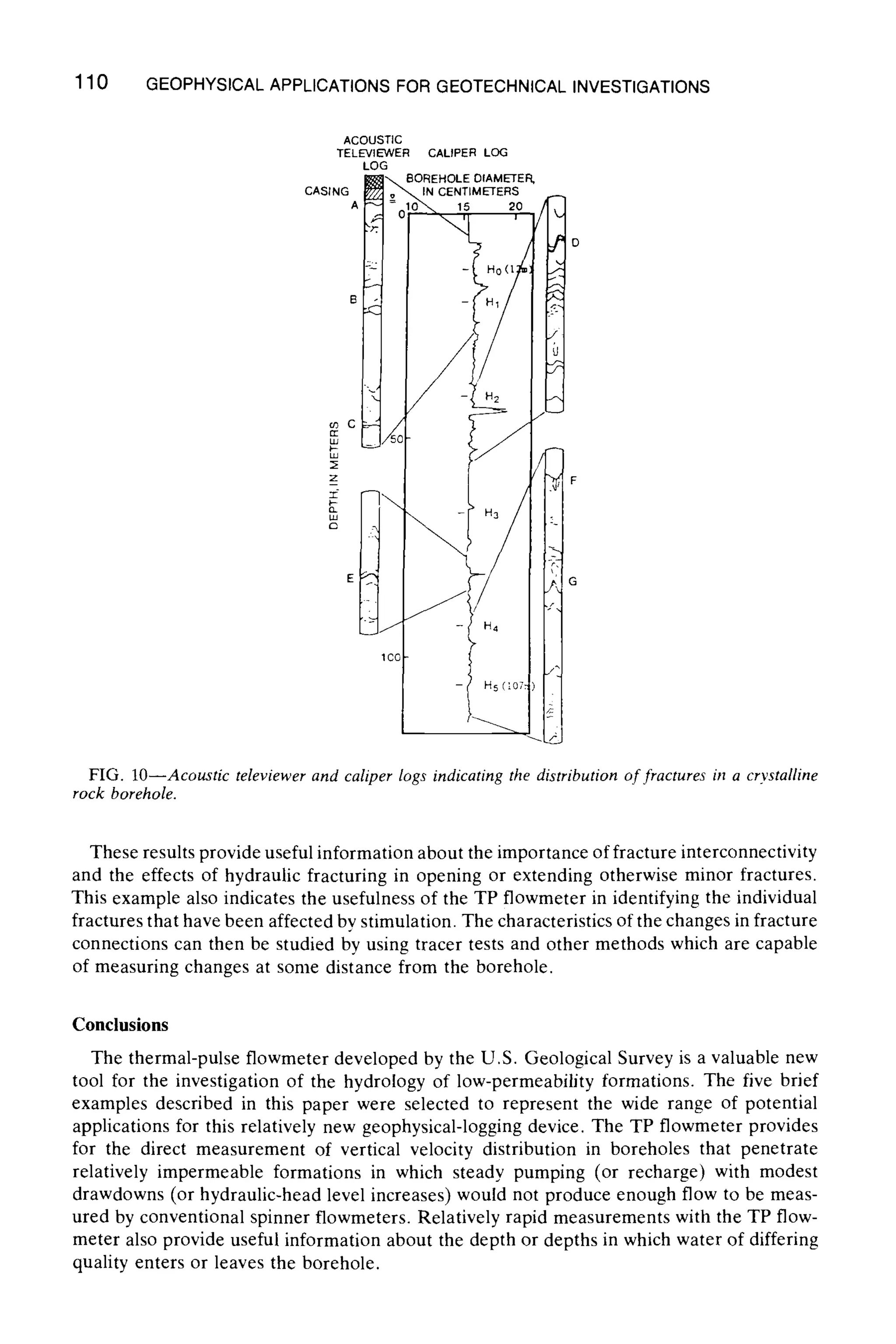
![HESS AND PAILLET ON THERMAL-PULSE FLOWMETER 111
o !21 I~
A, 1!: i
..............i B -
2o i 1 o
~, c
i
I
i
1
40 ,1
t
,
z_ , ~. z_
zff O' -
E6o ~', g .o~
= 1
80 [ 0
~ E "r
i
"F
i
I
i o
100 G ~ . o
i
12o ~ i ~LO 0 ~0 0 ~ 0 ~
oi ai ,-: .-: 6 d
DOWNFLOW,IN LITERS
FIG. 11--Verticalflow distribution in Borehole MO-1 determined with thermal-pulse flowmeter meas-
urements during constant-head injection before and after hydraulic fracture stimulation.
References
[1] Keys, W. S. and Sullivan, J. K., Geophysics, Vol. 44, No. 6, 1979, pp. 1116-1141.
[2] Schimschal, U., Ground Water, Vol. 19, No. 1, 1981, pp. 93-97.
[3] Morin, R. H., Hess, A. E., and Paillet, F. L., Ground Water, Vol. 26, No. 5, 1988, pp. 587-595.
[4] Hess, A. E., Canadian Geotechnical Journal, Vol. 23, No. 1, 1986, pp. 69-78.
[5] Hess, A. E., "Characterizing Fracture Hydrology Using a Sensitive Borehole Flowmeter with a
Wireline-Powered Packer," in Proceedings, American Geophysical Union/U.S. Geological Survey
Symposium on Fracture Hydrology, U.S. Geological Survey, Atlanta, GA, 1988, in press.
[6] Hess, A. E., "A Heat-Pulse Flowmeter for Measuring Low Velocities in Boreholes," U.S. Geo-
logical Survey Open-File Report 82-699, U.S. Geological Survey, Denver, 1982.
[7] Paillet, F. L. and Hess, A. E., "Geophysical Well-Log Analysis of Fractured Crystalline Rocks
at East Bull Lake, Ontario, Canada," U.S. Geological Survey Water Resources Investigations
Report 86-4052, U.S. Geological Survery, Denver, 1986.
[8] Paillet, F. L., Hess, A. E., Cheng, C. H., and Hardin, E. L., Ground Water, Vol. 25, No. 1,
1987, pp. 28-40.
[9] Paillet, F. L. and Kapucu, K., "Fracture Characterization and Fracture-Permeability Estimates
from Geophysical Logs in the Mirror Lake Watershed, New Hampshire," U.S. Geological Survey
Water Resources Investigations Report 89-4058, U.S. Geological Survey, Denver, 1989.](https://image.slidesharecdn.com/geophysicalapplicationsforgeotechnicalinvestigations-151104153926-lva1-app6892/75/Geotechnical-Geophysics-113-2048.jpg)
![112 GEOPHYSICALAPPLICATIONS FOR GEOTECHNICAL INVESTIGATIONS
[10] Davison, C. C., Groundwater Monitoring Review, Vol. 4. No. 4, 1984, pp. 95-102.
[11] Paillet, F. L., Log Analyst, Vol. 26, No. 6, 1985, pp. 26-41.
[12] Trainer, F. W., in The Geology of North America, Hydrogeology, Vol. 0-2, W. Back, J. S.
Rosenshein, and P. R. Seaber, Eds., 1988, pp. 367-380.
[13] Paillet, F. L., "Fracture Characterization and Fracture-Permeability Estimation at the Under-
ground Research Laboratory in Southeastern Manitoba, Canada." U.8. Geological Survey Water-
Resources Investigations Report 88-4009, U.S. Geological Survey, Denver. 1988.
[14] Hess, A. E. and Paillet, F. L., "Characterizing Flow Paths and Permeability Distributions in
Fractured-Rock Aquifers Using a Sensitive, Thermal Borehole Flowmeter." in New Field Tech-
niques for Quantifying the Physical and Chemical Properties of Heterogeneous Aquifers Conference,
Proceedings, F. J. Molz, J. G. Melville, and O. Guven, Eds., National Water Well Association,
Columbus, OH, 1989, pp. 445-461.
[15] Paillet, F. L., Waltz, J., and Boyle, R. E., "Geophysical Log Investigation of Formation Changes
Produced by Hydraulic Fracture Stimulation in a Crystalline-Bedrock Aquifer," in Proceedings,
Minerals and Geotechnical Logging Symposium, 1989, Minerals and Geotechnical Society. Las
Vegas, in press.
[16] Bredehoeft, J. D., Wolff, R. G., Keys, W. S., and Shuter, E., "Hydraulic Fracturing to Determine
the Regional In-Situ Stress Field, Piceance Basin, Colorado," Geological Society of America,
Bulletin, Vol. 87, 1976, pp. 250-258.
[17] Zoback, M. D. and Haimson, B. C., "Status of the Hydraulic Fracturing Method for In-Situ Stress
Measurements," in Proceedings of the 23rd Symposium on Rock Mechanics. American Institute
of Mining, Metallurgical, and Petroleum Engineers, Berkeley, CA, 1982. pp. 143-156.](https://image.slidesharecdn.com/geophysicalapplicationsforgeotechnicalinvestigations-151104153926-lva1-app6892/75/Geotechnical-Geophysics-114-2048.jpg)


This document provides an overview of a publication containing papers from the Symposium on Geophysical Methods for Geotechnical Investigations. The publication covers both surface and borehole geophysical techniques applied to environmental and geotechnical engineering problems. Surface methods provide horizontal maps or vertical profiles of subsurface properties, while borehole methods provide continuous vertical logs of properties along boreholes. Together, surface and borehole methods provide complementary data for characterizing geological formations and groundwater.