1. Seismic Reflection Methods Applied to Engineering,
Environmental, and Groundwater Problems
Don W. Steeples* and Richard D. Miller*
Abstract
The seismic-reflection method, a powerful geophysical
exploration technique that has been in widespread use in the
petroleum industry for more than 60 years, has been used
increasingly since 1980 in applications shallower than 30m.
The seismic-reflection method measures different parameters
than other geophysical methods, and requires careful attention
to avoid possible pitfalls in data collection, processing, and
interpretation. Part of the key to avoiding the pitfalls is to
understand the resolution limits of the technique, and to plan
carefully shallow-reflection surveys around the geologic
objective and the resolution limits. Careful planning is also
necessary to make the method increasingly cost effective
relative to test drilling and other geophysical methods. The
selection of seismic recording equipment, energy source, and
data-acquisition parameters is often critical to the success of a
shallow-reflection project. By following known seismic
reflections carefully throughout the data-processing phase
misinterpretation of things that look like reflections but aren't
is avoided. The shallow-reflection technique has recently been
used in mapping bedrock beneath alluvium in the vicinity of
hazardous waste sites, detecting abandoned coal mines,
following the top of the saturated zone during a pump test in
an alluvial aquifer, and in mapping shallow faults. As
resolution improves and cost-effectiveness increases, other
new applications will be added.
Introduction
The seismic reflection method which has been used for
underground exploration for over 60 years (Dobrin, 1976;
Coffeen, 1978; Waters, 1997) is being used in the 1980s for
targets shallower than 30m. Advances in microelectronics
have resulted in construction of engineering seismographs and
microcomputers that permit cost effective collection and
processing of seismic reflection data in numerous applications
Unique features of the seismic reflection method applicable
to shallow engineering, groundwater, and environmental
projects are described and recent applications are illustrated.
A nonmathematical discussion of seismic methods and the
differences between reflection, refraction, and borehole
seismology are given. The seismic reflection method is
compared with ground-penetrating radar. A set of high quality
shallow seismic reflection data *introduces the fundamentals
of seismic reflection and a seismic data processing discussion.
Pitfalls of data processing and interpretation are introduced,
including spatial aliasing, recognition of refractions in
reflection data, and problems with air-coupled waves. Because
successful use of the shallow seismic reflection method
requires proper field data acquisition techniques, a discussion
of geologic targets, site logistics, and parameter selection for
various situations is included. Differences in the criteria for
selection of seismic sources, seismographs, and geophones for
shallow surveys as opposed to deeper surveys are given.
Because the shallow seismic reflection method has not been
widely used in production, a short discussion of field data
collection efficiency and costs which could be of use to
contractors in the initial stages of planning a geotechnical site
investigation is provided. Case histories show file utility of the
shallow seismic reflection Method in detecting faults, cavities
and intra-alluvial stratigraphy. Use of the method in
characterizing geologic, hydrologic, and stratigraphic
conditions within 3m to 30m of the earth's surface is
increasing.
Seismic reflection techniques depend on the presence of
acoustical contrasts in the subsurface. In many cases the
acoustical contrasts occur at boundaries between
* Kansas Geological Survey, The University of Kansas Lawrence, Kansas

2. geologic layers, although man-made boundaries such as
tunnels and mines also represent contrasts. Acoustical
contrasts occur as variations in either mass density or seismic
velocity or both. The measure of acoustical contrast is
formally known as acoustic impedance, which is simply the
product of mass density and the speed of seismic waves
traveling within a material.
In the case of P-waves, which are compressional waves,
the principles of sound waves apply and, indeed, P-wave
reflections can be thought of as sound wave echoes from
underground. P-waves propagating through the earth behave
similar to sound waves propagating in air. When a P-wave
comes in contact with an acoustical contrast in the air or
underground, echoes (reflections) are generated. In the
underground environment, however, the situation is more
complex because some of the energy that is incident on a
solid acoustical interface can also be easily transmitted across
the interface or converted into refractions or shear waves
In the world of shallow geophysics, there are similarities
between seismic reflection, seismic refraction, and
ground-penetrating radar. There are also similarities with
cross-hole seismic tomography and vertical seismic profiling.
The similarities with electrical and potential fields methods
are substantially less. In particular, seismic methods are most
sensitive to the mechanical properties of earth materials and
are relatively insensitive to chemical makeup of both the
earth materials and their contained fluids. Electrical methods,
in contrast, are sensitive to contained fluids and to the
presence of magnetic or electrically conductive materials. In
other words, the measurable physical parameters upon which
tile seismic methods depend are quite different than the
important physical parameters for electrical and magnetic
methods.
It is somewhat of a paradox that seismic reflection
methods and ground-penetrating radar arc similar in concept,
but are almost mutually exclusive in terms of where they
work well. Both methods use reflections of energy from
underground features. Radar works well in the absence of
electrical conducting materials near the earth's surface, but
will not penetrate into good electrical conductors. The
seismic reflection method on the other hand, works best
where the water table is near the surface and easily penetrates
damp clays that are excellent electrical conductors. Radar
penetrates dry sands that will not easily transmit
high-frequency seismic waves.
The earliest work in the literature that convincingly shows
seismic reflections shallower than 20m is that of Schepers
(1975). While that pioneering effort resulted in excellent
data, it did little to encourage widespread use of shallow
seismic reflections. Thc work of Jim Hunter and Susan Pullan
and their colleagues at the Geological Survey of Canada
(Hunter et al., 1984; Pullan and Hunter 1985) and Klaus
Helbig (Doornenbal and Helbig, 1983; Jongerius and Helbig
1988) and his students at the University of Utrecht in The
Netherlands has been instrumental in developing shallow
seismic reflection procedures. In particular, Hunter's
optimum window-common offset technique has been widely
used since the simple data manipulation and display can be
done on an Apple II series microcomputer. Shallow CDP
seismic reflection profiling is becoming less costly, and
therefore, is increasingly used because processing of the data
can now be done efficiently on a PC/AT compatible
microcomputer (Somanas et al., 1987).
The Basics of Various
Seismic Methods
The purpose of this paper is not to present a thorough
explanation of exploration seismic methods, since this
explanation can be found in any basic textbook on
exploration geophysics (Dobrin, 1976; Telford et al., 1976;
Sheriff, 1978). It is important to know, however, that certain
similarities exist between various seismic methods, and what
the general limitations of the methods are. In all seismic
methods, some source of seismic energy is used and some
type of receiver is needed to detect seismic energy that has
traveled through some volume of the earth. In this paper we
will use geophones as receivers except where we explicitly
mention hydrophones or accelerometers.
Seismic Refraction
The seismic-refraction method requires that the earth in
the survey area be made up of layers of material that increase
in seismic velocity with each successively deeper layer. The
data analysis becomes more complicated if the layers dip or
are discontinuous. The requirement for increasing velocity is
a severe constraint for many shallow applications where
low-velocity layers are often encountered within a few meters
or tens of meters below the earth's surface. For example, a
sand layer beneath clay in an alluvial valley commonly has a
lower seismic velocity than the clay, so seismic refraction
cannot be used in such a situation without giving erroneous
results. The technique is cheap and often cost-effective in
those cases where it works. An excellent article by Lankston
(1990) Is included in this volume.
Seismic Cross-hole Tomography
Tomographic surveys use the same mathimatical
approach that has been so successfully used by the medical
profession in the development of three-dimensional imaging
within the human body with x-rays (computed axial
tomography or CAT scan). The technique depends on
measurement of traveltime for large numbers of ray paths through a
body of earth material. While the technique involves timing

3. ray paths between boreholes, it is common to time
surface-to-borehole and/or borehole-to-surface ray paths also.
The technique is computationally intensive, and is costly
because of the need for boreholes. It often gives a very
detailed velocity model between the boreholes, and does not
require any assumptions to be theoretically correct.
Tomography has been used to study the interior of the earth
from scales of thousands of kilometers to tens of meters
(Clayton and Stolt, 1981; Humphreys et al., 1984).
Vertical Seismic Profiling
The vertical seismic profiling (VSP) technique is seldom
used alone, but rather is used to provide better interpretation
of seismic reflection data. Use of VSP commonly requires a
string of hydrophones, 3-component geophones or
3-component accelerometers in a borehole, and a surface
seismic source located within a few seismic wavelengths of the
borehole. VSP allows accurate determination of one-way
traveltime to various geologic units and analysis of attenuation
and acoustic impedances which are needed for construction of
synthetic seismograms. The synthetic seismograms are then
used for comparison with seismic-reflection data to identify
specific geologic formations and to refine depth estimates of
those formations. References on VSP include Gal'perin,
(1974) Hardage, (1983), and Balch and Lee (1984).
Shallow Seismic Reflection
The seismic reflection technique involves no a priori
assumptions about layering or seismic velocity. However, no
seismic energy will be reflected back for analysis unless
acoustic impedance contrasts are present within the depth
range of the equipment and procedures used. The classic use
of seismic reflections involves layered geologic units. It is
important to note that the technique can also be used to search
for anomalies such as isolated sand or clay lenses and cavities.
The problems of resolving such relatively small volumes are
discussed later under Cavity Detection. The technique is
rapidly becoming more cost-effective which brings new
applications as resolution improves.
Shallow Seismic Reflection
Fundamentals
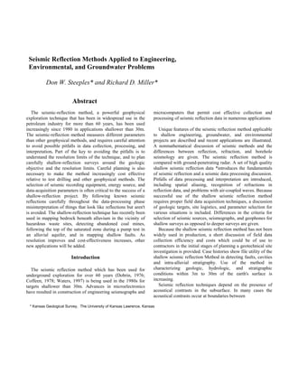
The simplest case of seismic reflection, a single layer over
an infinitely thick medium, is shown in Figure 1.
A source of seismic waves emits energy into the ground,
commonly by explosion, mass drop, or projectile impact.
Energy is radiated spherically away from the source. One
particular ray path originating at the source will pass energy to
the subsurface layer and return an echo to the geophone at the
surface first, following Fermat's principle of least time. In the
case of a single flat-lying layer and a flat topographic surface,
the path of least time will be from a reflecting point mid-way
between the source and the receiver with the angle of
incidence on the reflecting layer equal to the angle of
reflection from the reflecting layer.
In the real world, there are commonly several layers
beneath the earth's surface that are within reach of the seismic
reflection technique. Figure 2 illustrates that concept, but note
that the ray paths are in general not straight lines, but are
deflected at velocity discontinuities according to Snell's law.
The fact that several layers often contribute to seismograms
tends to make the seismic data more complex, since reflections
from greater depths arrive at later times than shallow
reflections. Complexity often also is increased by the presence
of seismic energy that has bounced one or more times between
layers in the subsurface (multiple reflections). In most cases,
refracted waves and P-waves that have been converted into
S-waves at subsurface interfaces also be present.
In the case of a multi-channel seismograph, several points
in the subsurface return reflected seismic waves to geophones.
Figure 3 shows a seismic-reflection record with a prominent
reflection from bedrock at 53ms which corresponds to a
bedrock depth of approximately 15m. Note in Figure 4 that the
subsurface coverage of the reflection data is exactly half of the
surface distance across the geophone spread. Hence, the
subsurface sampling interval is exactly half of the geophone
interval at the surface. For example, if geophones are spaced
at a 2m interval at the earth's surface, the subsurface
reflections
FIG. 1. The simplest case of seismic reflection. S represents the
source and R represents the receiver. Layer I represents an
acoustical discontinuity.

4. will come from locations on the reflector that are
centered 1 m apart.
In Figure 5 we have placed source locations and
receiver locations in such a way that path Sl-R2
reflects from the same location in the subsurface as
path S2-R I. This is variously called a
common-reflection point (CRP) (Mayne, 1962), a
common-depth point (CDP), or a common midpoint
(CMP) depending upon the preference of the author.
The power of the CDP method is in the multiplicity of
data that come from a particular subsurface location.
By gathering CMP data together and then adding the
traces, the reflection signal is enhanced. Before this
addition can take place, however, the data must be
corrected for differences in traveltime for the reflected
waves caused by the differences in source-to-geophone
distance (discussed in the following section). The
degree of multiplicity of data from a particular location
is known as "CDP fold.” A 24-channel seismograph,
for example, is commonly used to gather 12-fold CDP
data. From a theoretical standpoint, signal-to-noise
(S/N) ratio of reflections improves proportionally to
the square root of the CDP fold.
Reflections from Three Layers
FIG. 3. Field seismogram (unprocessed) showing bedrock
reflection at about 53 ms. The hyperbolic shape of the shaded zone
is characteristic of simple reflections. The earlier arriving energy is
from air blast and from direct arrivals passing through near-surface
alluvium. Geophone offsets are 3 rn for the inside two traces,
increasing to 16 m for the most distant traces.
FIG. 2. Reflected rays from three layers. In general the ray paths
are deflected from straight lines at boundaries between layers
according to Snell's law, so this figure is over-simplified
Simple Reflection Ray Paths
FIG. 4. Schematic view of reflection ray paths in a single layer
case for a six-channel seismograph. Note that the common
depth-point spacing is exactly half the geophone spacing.

5. FIG. 5. Illustration of the common-depth-point (CDP) concept. In
the case of a 24-channel seismograph with shotpoints occurring at all
geophone locations, the subsurface reflection points will be sampled
12 times, resulting in 12-fold CDP data after processing.
The purpose of the seismic-reflection method is to
determine the spatial configuration of underground
geological units. Figure 6 shows conceptually what we
are trying to accomplish with such a survey. Note that
the peaks of the seismic reflections have been
blackened to assist in the interpretation.
Obtaining high quality shallow seismic reflection data
is still somewhat of an art that is improved by
experience. In the following sections, we provide our
*ideas based on 10 years of experience practicing this
art and then we present several examples.
Processing Shallow Reflection Data
The purpose of processing CDP seismic reflection
data is to enhance the reflections at the expense of
everything else. A wide variety of filtering, display, and
static correction techniques can be employed to improve
the quality of the reflections. We will discuss only those
techniques that are necessary to understand the
fundamental CDP processing flow. There are many
places in the scientific literature to obtain more details
(Robinson and Treitel 1980; Waters, 1987; Yilmaz,
1987).
The raw seismic data are in a field file format with
each seismic trace for a particular shot stored according
to field file or shot point number and seismograph trace
number. Several steps are necessary prior to gathering
or sorting the data into a CDP format
The first step in actually processing the data is to
receive dead or unacceptably noisy traces by editing.
The next step in actually processing the seismic
reflection data is to make certain that each digital
seismic trace has a horizontal and vertical location and
distance from geophone to shotpoint explicitly
associated with it in a header. This header will allow for
elevation corrections and for properly sorting the data.
The data can then be sorted into CDP gathers such as
those shown in Figure 7. A CDP gather is a collection
of all seismic traces that, from a simplistic point of
view, have a common reflection point in the subsurface.
Note on these gathers in Figure 7 that there is a strong
reflection visible at about 60ms. True reflectors on a
CDP gather plotted
FIG. 6. Combining the 3-D geology with a conceptual seismic
section. The geology is interpreted from coherent blackened peaks
on the seismic section- Seismic data arc processed to emulate what
they would look like if the shotpoints and geophones were located at
the same point on the earth's surface.
FIG. 7. Common-depth-point gather at points 988 and 989 on
a particular shallow seismic survey. The most prominent
seismic wavelet at times between 50 and 70ms is a bedrock
reflection from about 9m below the surface. The geophone
offsets were 3.7m (12 ft) for the nearest traces and 17m (56 ft)
for the farthest trace with 1.22m (4 ft) between geophones.

6. with traces in order of increasing or decreasing
distance from the shotpoint, have a hyperbolic
curvature to them as can be seen on Figure 7. The
degree of curvature of the hyperbola is determined by
the average seismic velocity above the reflector, depth
to the reflector, and distance from the shotpoints to the
geophones and is also dependent on dip of the
reflector and topographic slope at the earth's surface.
A trace-by-trace depth and distance-dependent time
shift must be made to each trace to correct for
nonvertical incident rays prior to the stacking of the
CDP gathers. The next step is to determine the seismic
velocity within the materials penetrated by the
reflected seismic waves. The simplest procedure with
good seismic-reflection data is to fit a hyperbola to the
data using a least-squares approach. Table 1 shows a
simple program for a HP11C or HP15C calculator that
will calculate seismic velocity for such a case. The
user simply inputs two or more time-distance pairs of
numbers from a reflection on the field record or from
the CDP gathers to calculate a seismic velocity. The
program also calculates the reflection time for the
zero-offset distance for the hyperbola. Note in Figure
6 that the data have been displayed as though the
distance between shot and geophone were zero. This is
known as zero-offset (vertical incidence) and the data
are processed to approximate the zero-offset (or ideal)
case.
Another approach is to have the seismic processing
computer apply a series of constant velocities to the
field records or the CDP gathers. The velocity that
flattens the reflector the best represents the best NMO
velocity for that CDP (Figure 8) at that particular
two-way reflection traveltime.
Table 1. Shown is a program that will run on either an HP I IC or HP 15C pocket calculator. The program (1) uses two or more
time-distance pairs (distance treated as x and time as y) measured from a field seismogram as input data; (2) performs an hyperbolic
least-squares fit of the data, assuming the time-distance pairs are picked from a true reflector; (3) calculates, stores, and displays zero-offset
reflection time (TO), velocity (Vnmo), depth to reflecting interface (z), and correlation coefficient (r). The program assumes flat-lying as
opposed to dipping reflectors. Test data: T1 = 0303 s, X1, = 0.5 m; T2 = 0.0305 s; X2 = 1.5 m; T3 = 0.032 s; X3 = 2.5 m. For these test data:
To stored in register R8 - 0.03006 s; Vnmo stored in register R9 - 232.6 m/s; z stored in register R.0 = 3.49 m; r stored in register R.1 = 0.974
.
Keystroke g P/R to get the calculator into program mode, then
input the keystrokes as indicated- After inputting the program,
keystroke g P/R to get back to operating level, then keystroke f
USER to get to USER mode.

7. An extension of this technique is done by stacking
several of the constant-velocity gathers for a group of
CDP's into a constant-velocity CDP stack (Yilmaz,
1987).
A cross-correlation technique has been developed
by Taner and Koehler (1969) to determine the best
NMO velocity. The technique allows careful objective
consideration of several velocity values over a large
time window and a large number of traces while
requiring a minimum amount of personnel time.
After the velocity has been determined, the NMO
correction is applied to all of the data. For shallow
surveys, it is common to have a velocity model
composed of only one low-velocity layer over a large
thickness of high-velocity bedrock. We have found
that velocity in the shallow layers often varies
drastically and abruptly with horizontal location.
Consequently, we commonly process data using a
single layer with laterally varying velocity above an
homogeneous thick bedrock. For deeper surveys, it is
common to have several layers in the velocity model.
At this point in the processing flow, we have sorted
the data into CDP gathers and corrected for difference
in source-to-geophone distance. We are now ready to
sum all of the traces together within each CDP gather.
Figure 9 shows five traces of CDP stacked data in
which each stacked trace is composed of the
post-NMO sum of twelve traces from CDP gathers
like those shown in Figure 7.
Figure 10 shows the same five traces of CDP
stacked data processed at three different test
velocities. Note that the correct velocity gives the
highest frequency and

8. FIG. 8. Velocity analysis on CDP gather at point 988 from Figure
7. Note that 1075 ft/s (328 m/s) is too slow and the moveout is too
great on the far traces. A velocity of 1225 ft/s (373 m/s) nicely
flattens the reflection signals in preparation for adding the traces
in the computer. A velocity of 1375 ft/s (419 m/s) is too fast and
does not provide enough moveout on the far traces to flatten the
reflection signals.
the best coherency on the stacked data. It is also
important to realize that the correct velocity is the
only velocity that puts the reflector at its correct
depth. In other words, stacking CDP data with the
wrong velocity hurts the resolution of the data,
decreases the S/N ratio, and results in the wrong
time-location on the final stacked sections.
While the wrong velocity hurts the data quality,
there are other shallow reflection pitfalls that can lead
to grossly incorrect interpretations. Some of the most
basic of the many possible pitfalls arc discussed in the
following section.
Some Pitfalls of Shallow
Seismic Reflection
The principles of shallow CDP seismic reflection
are shown in Figures 1 through 10, inclusive. While
the principles are not difficult to grasp, there are
several pitfalls of shallow seismic reflection that
should be presented. We have seen several examples
during the past few years where seismic reflection
interpretations have been ascribed to seismic data
composed of refractions, ground roll, air-coupled
waves, and/or just plain noise.
FIG. 9. Five traces of 12-fold CDP stacked data showing
bedrock reflection at about 50 ms. Each trace has had 12 field
traces added together after they were individually adjusted by
applying velocity-distance normal-moveout (NMO) based on the
velocity analysis of Figure 8. Distance between CDP traces is 0.61
m (2 ft).
FIG. 10 The five 12-fold CDP traces of Figure 9 are shown
processed with three different velocities. Note that when the
velocity is too low, the frequency of the reflection wavelet is
lowered and is therefore depicted too shallow on the seismic
section. When the velocity is too high, the frequency decreases
and the reflection wavelet is depicted too low on the seismic
section. The correct velocity gives the correct position for the
wavelet and preserves the high frequencies which allows best
resolution of small features and thin beds. Correct velocity is
about 373 m/s (1225 ft/s).

9. While to our knowledge none of these occurrences has been
published in the refereed scientific literature, some of them
have been in geotechnical advertisements and others have
been in consulting reports and unrefereed conference
proceedings. We believe that one of the biggest obstacles to
widespread use of shallow seismic reflection in the next
decade is the potential misuse by those who fail to appreciate
and understand the pitfalls of the technique.
Substantial progress has occurred during the past ten years
in development of shallow seismic reflection techniques.
Hunter's optimum-window technique (Hunter et al., 1984) is
now widely and routinely used in engineering and
groundwater applications. Our own research has focused on
probing the limits of the resolution and the applications of
shallow seismic reflection using common-depth-point (CDP)
techniques and extensive routine digital processing. Both
approaches to shallow seismic reflection profiling have
potential for misuse by individuals without substantial
training and experience. Some of the pitfalls of the methods
and how to avoid them or at least decrease the chances of
erroneous interpretations are illustrated. We present
examples of data that have been or could easily be
misinterpreted as seismic reflections. Problems that often
occur are spatial aliasing of ground roll, interpreting the
ground-coupled air wave as a true seismic wave, and
misinterpreting shallow refractions as shallow reflections in
stacked CDP sections.
Spatial Aliasing
Aliasing occurs when data are not sampled often enough
in time and/or space. For instance, buggy wheels appear to
turn backward in western movies even though it is obvious
that the buggy itself is moving forward. This phenomenon
occurs because the movie camera does not sample the
viewing field often enough to depict accurately what
actually occurred. If aliasing can make buggy wheels appear
to turn the wrong direction, imagine how seriously aliasing
might affect seismic data.
Figure 11 shows a seismic field plot from the Hobble
Creek, Utah, vicinity. Note that an apparent reflector is
present near the arrow at about 55 ms. While this is not the
best appearance of a shallow reflector that has ever
occurred, it is certainly suggestive of a reflector. Note in
Figure 11 that the geophone interval is 1.28 m. Now look at
Figure 12 which was recorded at the same shot-point with
geophone spacing of 0.64 m. All parameters and locations
are the same on Figures 11 and 12 except that the geophone
interval is cut in half for Figure 12. In fact, Figure 11 is
Figure 12 with the even traces removed. Note on Figure 12
that the apparent reflector is nowhere to be seen. When we
first fired a test shot at this site with 1.28-m geophone
spacing, we thought we were seeing a reflector. Cutting the
geophone spacing by a factor of two for the next test shot
quickly cleared up that misconception. Clearly, the apparent
reflector in Figure 11 is not a reflector at all, but is spatial
aliasing of ground roll.
We have noted the occurrence of spatial aliasing of
ground roll at other sites, also. The unsuspecting
seismologist might take such data and build a whole survey
around it only to wonder later why the "reflector"
disappeared in processing or, worse yet, might plot
common-offset ground roll as an interpreted reflection. We
have developed a few tricks to help avoid that trap.
(1) If it is a true reflector, moving the shotpoint one-half
geophone interval closer to (or further away from) the
geophone spread will have essentially no effect on the
appearance of the reflector. If it is spatial aliasing of
ground roll, the effect is usually substantial.
(2) Decreasing the geophone interval by a substantial
amount (such as a factor of two or three) will improve
coherency of a true reflector, but will destroy
coherency of spatially aliased ground roll.
(3) If something is known geologically about the site (such
as uphole traveltime, depth-to-bedrock, etc.), it is
possible that the geologic information can be used to
determine when the reflection should be expected on
the record and what its normal moveout (NMO) should
be. As mentioned earlier, Table 1 shows a HP-11C or
HP-15C calculator program for calculating a
least-squares-fit hyperbola to a set of T and X points
measured directly off a field seismogram. The inputs to
the program are two or more arrival times of the
suspected reflector along with their corresponding
shot-to-geophone distances. The program solves for
NMO velocity, intercept time (TO), depth-to-reflector
interface, and correlation coefficient of the reflection
hyperbola to the data points. Remember that the
correlation coefficient is meaningless unless three or
more time-distance measurement pairs are included as
inputs. The output from the program can be of
tremendous help in field analysis of seismograms
regardless of whether the reflections are real or just
apparent. Our experience with this program suggests
that the correlation coefficient should be 0.99 or larger
if three of four time-distance pairs are used for the
calculation. For coefficients less than 0.99, either the
energy is probably from ground roll rather than from
reflections the data are of poor quality, the reflection
was not real, major static correction problems are
present, or there is dip or structural complexity
indicated on the individual seismogram.
(4) Reflected energy from shallow depths tends to have a
frequency content close to that of the direct wave or
early refracted arrivals. If the observed frequency on
displayed common offset or CDP sections is much
lower than the first arrivals, then the energy is probably
from ground roll rather than from reflections.

10. FIG, 11. The event shown by the arrow at 55 ms could be
mistaken for a reflection. See Figure 12 for comparison
FIG. 12, Note the coherent event at 55 ms from Figure I I is no
longer apparent. Figure 11 is actually Figure 12 with the even
traces removed- The coherent event on Figure I I at 55 ms is
spatially-aliased ground roll.
Ground-coupled Air Wave
Figure 13 shows an example of a CDP seismic
section from near Heber City, Utah. Reflectors
corresponding to times of 20 to 40 ms have been
verified by drilling. Apparent reflections at 60 to 70
ms are ground-coupled air waves, and are not true
reflections at all. Experience has shown that the air
wave tends to have a frequency near that of the
low-cut filter - 220 Hz in this case. We were using a
geophone group interval of 1.52 m during the
collection of this data set. Note that 1.52 m multiplied
by 220 Hz gives a velocity of 335 m/s which is
exactly the velocity of sound in air at 6o
C. In other
words, our field setup was accidentally designed
perfectly to develop a 360-degree phase shift of the air
blast from trace to trace on field data. The air blast
was a double sinusoid that stacked quite nicely on the
processed sections.
The ground-coupled air wave is a problem With
many types of sources including hammers and weight
drops. Particularly when reflections are needed in the
upper 30 ms of record, the echoes in the air can easily
be recorded on the seismograms. Miller et al. (1986)
had major problems with air-coupled waves echoing
from trees during a series of source tests for shallow
sources. Almost all of the sources had that problem.
Recordings of the ground-coupled air wave are
recorded for the widely-held but mistaken belief that
seismic P-wave velocities of less than 330 m/s are not

11. Fig 13. Twelve-fold CDP section showing intra-alluvial reflectors
in upper 30 ills. Apparent reflection between 60 and 70 ms is air
blast from Betsy seisgun. Distance between traces is 1.52 m (5 ft).
observed in near-surface materials. In Figure 26, for
example, the ground-coupled air wave arrived first,
but the direct wave through the ground arrived with a
P-wave velocity of only 260 m/s.
Refractions
It is exceptionally difficult to separate shallow
reflections unequivocally from shallow refractions
(Figure 14). Refractions on a stacked section tend to
be a bit lower in frequency because the NMO
correction in a CDP stack assumes hyperbolic
time-distance moveout, while refractions arrive as a
linear time-distance function. Hence, they don't stack
as coherently as reflections, which tends to decrease
their frequency. Figure 14 shows what appear to be
reflection events from 20 ms to 125 ms. However,
careful examination of the field data suggests coherent
events on the CDP stack shallower than 40 ms
resulted from refracted arrivals. Furthermore, test
drilling, geophysical logging and all uphole shot show
that the event at 75 ms is a true reflector from a
sandstone-limestone interface at a depth of 46 m. The
apparent 40 ms and 25 ms reflectors should be viewed
with suspicion for at least two reasons. Their lower
frequency and larger amplitude raise doubts as does
the fact that 3 ms of apparent structure in a horizontal
distance of 8 m suggests local apparent dip of about
17 degrees which is not geologically reasonable at this
locality.
One of the common uses of shallow seismic
methods is mapping depth to bedrock. Note that
refractions and reflections respond in the same way to
an increase in depth to bedrock. Hence, if refractions
stack in on a CDP seismic section, they can sometimes
lead the interpreter to a bedrock channel. The danger
is in thinking that the interpretation is correct in the
reflection sense because it was "confirmed" by
drilling. In reality, it may just be that the refractions
arrived later above the channel.
Our experience has been that occasional field
records display unusually good reflections. These
field seismograms can be used to correlate to the
sections. In all of our reports and published papers, we
include at least one field seismogram to show that the
reflections are real. When reviewing similar works
prepared by others, we always like to see a field
seismogram to verify that the “reflectors” are not
refractions and were not manufactured during
processing.
Refracted arrivals should be muted during the early
stages of the processing to remove any chance of them
stacking in on the section. Unequivocally separating
shallow reflections from shallow refractions is clearly
one of the major limitations of the shallow seismic
method at the present time
Planning Seismic Data Acquisition
Geologic Target
Some of the discussed pitfalls can be minimized by
careful planning, especially using the
optimum-window technique of Hunter et al. (1984).
The first step in planning a shallow seismic reflection
program, however, is to define the geologic target.
This definition includes an estimate of the typical
depth to the target, preferably within a factor of two,
by whatever means are available. The interval of
interest must be determined as well as whether
reflection data might be expected to show one of more
reflectors within that interval. The means available
may include limited drilling information, nearby
outcrops of some layers, and previous geologic and
geophysical reports on an area. By no stretch of the
imagination should a shallow seismic reflection
survey be the first geotechnical investigation of an
area, so do the homework first as part of the planning
process.
Once the geologic problem has been defined by the
above process, the attainable limits of vertical and
horizontal resolution should be considered. For

12. example, is it possible to resolve a 1 m thick sand lens
within the

13. Reno, Kansas Test Site
Effect Of Improper First-Arrival Mute
12-Fold CDP Stack
Source: 30.06 Rifle
Low-Cut Filter (pre A/D): 220 Hz
FIG. 14. Seismic section showing how refractions can stack in as
apparent reflections if not properly muted during processing.
Coherent events between 25 and 45 ms are refractions instead of
reflections. Distance between CDP traces is 0.61 m (2 ft).
clay, or is it possible to detect a solution cavity that
is likely no larger than 5 m in diameter? These
questions are discussed in some detail in Widess
(1973), Sheriff (1980), and Knapp and Steeples
(1986a). Briefly, bed thickness of at least one-quarter
wavelength is needed to effect vertical resolution,
while the horizontal dimensions of a feature must
approach the dimension of the first Fresnel zone for
reliable resolution of the feature.
If preliminary planning considerations suggest that
shallow seismic reflection might work, then consider
the depth accuracy that is necessary for success of
the project. In some cases depth accuracy is
important only in the relative sense, such as finding
the deepest part of a buried valley. In other cases,
depth may be a secondary consideration and the
primary interest may be detection of a fault, for
example. In still other cases, the absolute depth may
be critical. If the absolute depth is critical, an error
analysis is appropriate. Errors occur in visual timing
of the seismic records, in determining shot initiation
time, in velocity analyses, in determining static
corrections, and in surveying surface locations. This
phase of the planning process will reveal the
accuracy with which things must be done in the field,
or that sufficient accuracy cannot be attained at all
with seismic-reflection methods.
Site Logistics
Site logistics must be considered before deciding
on field recording parameters. For example, we once
performed a seismic reflection survey for a railroad
that required mounting the recording truck on a work
train which had to be moved to a siding six miles
away several times a day to allow freight trains to
pass. Questions of vehicle accessibility can vastly
affect the rate at which seismic work can progress. In
some cases it may be necessary to pack all of the
equipment in on foot or by helicopter. These
considerations all factor into the selection of energy
source and other equipment.
At some locations, cultural considerations may be
an overriding factor. We have found that working
near Denver's Stapleton Airport requires waiting
about 10 percent of the time for jet aircraft noise to
subside to acceptable levels on the seismic data
(Figure 15). Other sources of cultural noise include
traffic and construction work nearby. Since most of
the noise generated by these

14. sources is below 100 Hz, and higher noise
frequencies are selectively attenuated quickly by the
earth, the use of low-cut filters is an effective way of
minimizing the problem. The MiniSOSIE (Barbier et
al., 1976) method is one option for attaining
frequencies up to approximately 100 Hz in areas of
intense, continuous cultural noise. We were able to
obtain useful seismic reflection data in the median of
Interstate Highway 80 in Salt Lake City in the
continuous presence of six lanes of heavy traffic with
the MiniSOSIE method.
Pipelines and power lines are a particularly
troublesome source of 60-Hz noise and sometimes
mechanical noise when they are buried in the vicinity
of a seismic line. One pipeline problem we
encountered during work in Winter Park, Colorado,
involved a vertical vent tube for the Moffet water
tunnel (Figure 16). Occasionally a pipeline that is
FIG. 16. Noise from pipeline vent tube which is located at the
asterisk at the top of the field seismogram. Note true seismic data
are visible between times of 60 and 80 ms on the left half of the
traces. Distance from shotpoint varies from 61 rn (200 ft) to 90 in
(296 ft).
cathodically protected with 60 Hz power running
through a half-wave rectifier can produce substantial
120 Hz and higher mode noise on seismograms. The
good news for shallow seismic reflection surveys that
employ low-cut pre-A/D filters of 200 Hz or higher is
that 60 Hz noise is usually pretty well wiped out. We
have worked directly beneath huge power lines in a
major power substation in the Los Angeles area using
220 Hz pre-A/D low-cut filters in conjunction with
factory installed 60 Hz notch filters and found that 60
Hz noise was not a major problem.
There are many natural environmental factors that
should be considered in the planning phase. The
presence of such things as brush, streams, and
boulders can affect the ability to plant geophones and
operate seismic sources along the planned seismic
line(s). Elevation relief is particularly critical in the
case of shallow seismic lines where the depth to the
reflector may be no more than a few times greater
than the relief. For example, surface relief of 5 m
along a shallow seismic line with a target depth of 20
m is equivalent to a 500 m relief problem along a
seismic line with a target depth of 2000 m. In fact,
the problem is often even worse for shallow surveys
because the velocity in the upper 5 m often varies by
a factor of two within a very short horizontal distance
for reasons that are not apparent at the earth's surface.
Our experiments indicate that good data quality is
also strongly dependent on the absence of
near-surface relatively thin high-velocity layers
(Figure 17). Note that the reflection quality is
excellent beneath the alluvium and terrible beneath
the limestone layer. We believe that the edge of the
thin limestone is a key to the poor data on the left
half of Figure 17. Figure 18 is a walkaway-noise test
that shows a ringy wavelet in the vicinity of the
limestone outcrop, which illustrates the problem.
Other natural factors include wind, precipitation,
and temperature extremes. These factors can affect
the time of completion of a job, quality of data, and
the equipment needed for working comfort of
personnel. In some engineering seismographs, the
amplifiers develop substantial thermal noise when
subjected to working temperatures above 100o
F.
Remember that when ambient temperatures outside
are 100o
F, temperatures inside a vehicle may be
somewhat higher and the temperature inside a closed
seismograph may be sufficient to induce malfunction.
Some tape and disk drives don't work well when
temperatures are below freezing. Wind is a major
source of noisy seismic data, although burying

15. geophones is a common (and expensive) way to try to
decrease the
FIG. 17. Twelve-fold CDP section from near Lyndon, Kansas,
showing the importance of near-surface geology to data quality. The
presence of the near-surface thin-bedded limestone is thought to be
the key to the poor data quality on the left twothirds of the section
(data courtesy of Andrew Kalik, Kansas Geological Survey).
Distance from outcrop varies from zero to 107 rn (350 ft). Elevation
of geologic section shown is between 305 rn (1000 ft) and 312 m
(1025 ft).
effects of wind. We have had better success in hooking two
single 100 Hz geophones in series at a distance of 1/2
wind-noise wavelength apart and aligned parallel with the
wind direction (Myers et al., 1987) than by burying
geophones. The wind noise wavelength can be determined by
aligning geophones parallel with the wind and measuring tile
wavelength directly from the resulting noise-test seismogram.
Air blast is a problem for virtually every surface seis-
mic source. Figure 19 shows a 12-fold CDP stack of an
intra-alluvial reflection survey near Manhattan, Kansas.
Note that near CDP 250 a diffraction pattern is apparent
at 55 ms. This diffraction pattern is actually in air-blast
echo from the recording truck. At the right side of the
figure the similar pattern at CDP 300 is also from the
echo from a later truck location. Similar echoes come
from buildings and trees.
Noise from even a sprinkle will show up on
seismograms. Figure 20 shows raindrop noise from a
shower that occurred during field work near Winter
Park, Colorado. Although we have not done exhaustive
analyses on the raindrop noise,
FIG. 18. Walkaway-noise test at Lyndon, Kansas field site of
seismic section from Figure 17. Note the variation of seismic
phases and possibly modes in the central third of the data at
times between 75 and 130 ms. The complicated geology in the
vicinity of the limestone outcrop contributes substantially to
the complications on the field seismograms (data courtesy of
Andrew Kalik, Kansas Geological Survey). Spatial dimensions arc
identical to those of Figure 17.
we believe it is caused by the geophones detecting the
air-coupled wave, since the noise is detected by several
geophones. Precipitation also usually causes leakage of
geophone signal-to-ground, particularly at points where
grass or weeds touch the connection of the geophone
clips or the cable takeouts. This leakage can cause
severe channel cross-talk and decreased S/N ratio. We
have alleviated that problem by using plastic dish pans
to elevate the cable-geophone connections above the
ground. Also, in the interest of
safety, a grounded seismic cable appears to an
imminent lightning bolt to be a nice linear receiving
antenna. The danger of lightning strike must not be
underestimated.
Acquisition Parameters
The selection of acquisition parameters varies with
the field experience of the seismologist in similar
geologic

16. FIG. 19. CDP seismic section from alluvial valley near Manhattan,
Kansas, showing air-blast echo from recording truck at time of 60
ms centered near CDP 250 and near CDP 300. The prominent
reflector at 55 ms is all intra-alluvial reflection that has been verified
by drilling and an up-hole shot time. Section is 61 m (200 ft) wide.
FIG. 20. Unprocessed field seismograms showing noise from
raindrops falling near the seismic line. On file 27 a raindrop impact
is obvious on the middle traces at times between 185 and 215 ms.
Other raindrops are obvious on the other field seismograms also.
Distance between traces is 0.6 m (2 ft).
situations. If a similar survey had been done by the
same seismic crew last year just down the road a couple
of kilometers, the parameter selection may be as easy as
looking in last year's field notes. Even in this case, we
find that our field techniques improve gradually but
continually. For that reason it is wise to run a
walkaway-noise test, a procedure that should not take
more than an hour or two in an area where the
seismologist has previous experience. Figure 21 shows
a typical walkaway-noise-test record for a
shallow-reflection survey.
A walkaway-noise test is conducted by setting closely
spaced geophones very near a test shotpoint. After the
first test shot, the geophones are moved progressively
farther from the test shotpoint and another test shot is
fired. This process is repeated until the investigator is
satisfied that all possible shotpoint-geophone offset
distances of interest have been tested. For target depths
of less than 30 m, we commonly use a 0.25 m geophone
interval for a walkaway-noise test. A useful
rule-of-thumb is to divide the primary depth of interest
by 100 and use that value for the walkaway-test
geophone interval. If
FRANKLIN CO.. KANSAS. WALKAWAY
DOWNHOLE 30.06
340 HZ (PRE A/D) LOW-CUT FILTER
SINGLE 100 HZ GEOPHONES
FIG. 21. Walk-away-noise test in Franklin County, Kansas. Note
the air-blast that runs diagonally across the figure from upper left to
lower right. The air blast is not present on the inner 24 traces which
were recorded on the first shot of the walkaway. On the first shot
exceptionally good source-to-ground coupling allowed recording of
reflections with dominant frequencies in excess of 300 Hz at times
of at least 140 ms, corresponding to depths of about 200 m. The
coupling on subsequent shots was not as good and data quality is
noticeably degraded. Distance from shotpoint is from 0.6 m (2 ft) to
73 m (240 ft) with 0.6 m (2 ft) between traces.

17. the nearest geophone is placed less than a meter from
the shotpoint, this has the effect of giving the
investigator 100 traces of seismic data to look at with
offsets less than the depth of interest.
To some degree the field parameters will be dictated
by the equipment available. For example, the number of
recording channels is often fixed by the seismograph,
and the cables and geophones may be limited by what is
on the shelf unless there are time and funds to rent or
purchase new equipment.
The geologic considerations addressed earlier will
dictate how long (in time) the seismograms will be. For
many shallow applications a time length of 100 ms is
plenty, giving records to depths of 30 m or more in most
localities. On seismographs that record data into
random access memory (RAM), there is often a
trade-off between record length and sample interval,
since the total amount of RAM may be fixed by
hardware or read-only memory (ROM). Once the
sample interval is selected, an anti-alias high-cut filter
must be selected to avoid aliasing of high frequencies to
low frequencies. We have already noted how aliasing
can make buggy wheels appear to turn backward in
Western movies. It is possible to use rather gentle (24
dB/octave or less) analog high-cut filters for
anti-aliasing purposes, but the industry standard seems
to be a high-cut filter that is down 60 dB at the alias
frequency. This is not so critical when using sample
intervals of 1/4 ms or less since there is very little
seismic energy present above the alias frequency of
2000 Hz. This would be critical if the seismograph or
any part of the seismic system had significant noise
levels at frequencies above the alias frequency.
The selection of high-cut filters is not usually critical
in shallow seismic surveys once any potential aliasing
problem is solved. We usually record with high-cut
filters out unless there is some strong source of
unwanted high-frequency noise. Provided the
high-frequency noise is not saturating the A/D
converters, it can always be filtered out later with a
digital filter that allows the processor to be selective in
terms of passband.
The selection of low-cut filters, on the other
hand, isone of the most critical decisions for a shallow
reflection project. The earlier discussion of geologic
requirements will dictate to some degree what
frequency must be attained to meet the survey
objective. In some cases, field testing will show that it
is not possible to meet that objective. We usually test
three or more low-cut filter set tings during the early
stages of the walkaway-noise test. We select the filter
setting that gives the best quality data in terms of
allowing us to meet the survey objective.
Sometimes a 340 Hz low-cut filter will make the data in
the upper 50 ms look great, but will not allow the
imaging of reflectors below perhaps 70 or 80 ms. In that
case, if our objective is below 70 ms, we back the low-
cut filters out to 220 Hz, or whatever value is required
to see reflections below 70 ms. Sometimes it is just not
possible to meet the survey objective, and it is best to
go home and seek cold refreshment.
Any analog filter that contains a resistor-capacitor
circuit will cause some phase distortion in the seismic
signals. That is, the time required for the signal to pass
through the filter is frequency dependent. If the
reflections from the objective depth do not change very
much in frequency from one part of the line to another,
phase distortion may not be a major problem. In such a
case, phase distortion merely decreases the apparent
frequency on CDP sections and amounts to very nearly
a static shift downward in time on the sections which
can cause small errors in absolute depth calculations. If,
on the other hand, the frequency of the reflections is
strongly location dependent, then phase distortion can
lead to incorrect interpretation of seismic sections. Such
frequency-dependent time shifts can be misinterpreted
as geologic structure. If the seismic data processor
knows the phase response of the analog filter-amplifier
combination used for recording, the data can be
dephased during processing. Phase distortion has not
been a major problem for us at frequencies below 300
Hz, but it could be a major problem as frequencies
approach I kHz or higher.
In most shallow applications, civilization is not far
away. Whenever civilization is nearby there will be
some 60 Hz noise present (50 Hz in Europe and some
other places) from the electrical power system. Also, if
a portable power generator is used it can cause major 60
Hz noise problems. Since a notch filter will cause some
phase distortion of the seismic data, it is best not to use
it if there is no 60 Hz noise visible to the naked eye on
the seismograms. As mentioned earlier, the low-cut
filters that are commonly used in shallow reflection
surveys may negate the need for notch filters. If the 60
Hz signal is clearly visible throughout the seismic
record, then the use of notch filters is clearly advisable.
The selection of amplifier gains usually takes several
test shots in the field, depending on the experience of
the individual operating the seismograph. In general the
gains should be set as high as possible without
saturating the A/D converters. In some cases, the data
will look better on field plots if the full digital word is
not used - particularly if strong wind noise or thermal
noise from the amplifiers is present. If the data are to be
digitally processed later it is usually better to go ahead
and use

18. the higher gains in the field to take full advantage of
the dynamic range of the seismograph, since the gains
can always be turned down digitally on playback after
processing to make the noise look smaller. Another
option is to increase the source energy to improve the
S/N ratio.
Some seismographs have specialized features that
allow the seismologist to be creative in choosing
parameters. For example, suppose that your
seismograph can only record 125 ms of data at the
sample rate you want to use. If your seismograph has a
"record start delay" feature, you can delay the start of
the recording process for a period of time after the shot
to allow you to look at data below 125 ms. In many
cases the data in the first 10 or 15 ms are not used
anyway. This allows you to look at reflection times to
depths of 135 to 140 ms without changing to a slower
sample rate and without losing useful data.
Another useful feature is "amplitude scan delay"
which can either be incorporated within the
seismograph itself or can be calculated in the field with
a portable microcomputer that reads the digital
seismograms from the seismograph in the field. This is
useful when the reflection event you want to see has
lower amplitude than the first arrivals or than the air
blast from the source to cite two examples. The use of
amplitude scan delay allows the observer to look only
at amplitudes deeper in time than some preset value.
For example, suppose that your target reflector is at
about 60 ms and that strong first arrivals are clipping
the data (saturating the A/D converters) in the time
range between 20 ms and 40 ms on all traces. It is
possible to set the amplitude scan delay at 50 ms which
allows clipping of data in the upper 50 ms but also
allows the observer to control the gains to prevent
clipping of the reflector or other signals at times greater
than 50 ms.
Selection of Geophones
The selection of seismic receivers is among the most
critical of decisions. For high resolution shallow
surveys, it is necessary to have receivers that are
designed to detect high frequencies without distortion
in the output signal. The first rule of thumb is to choose
a receiver with a natural frequency that is at least 10
percent of the highest frequency likely to be commonly
recorded. If the highest frequency likely to be recorded
is 400 Hz, then 40 HZ geophones might be sufficient.
The problem with lower frequency geophones is that a
phenomenon known as parasitic resonance tends to
occur within the geophone when substantial amounts of
seismic energy are present at frequencies more than an
order of magnitude above the natural frequency of the
geophone. Vertical geophones are particularly
susceptible to parasitic resonance when they are not
planted with their axis of movement very nearly
vertical.
Geophones have a response peak at their natural
frequency that can cause ringing in the data and an
artificial peak in the spectrum of the recorded data. To
counter this, damping resistors are used to flatten this
peak relative to the other response frequencies of the
geophone. The damping resistors also have the effect of
decreasing the sensitivity of the geophone at other
frequencies as well, which is sometimes not desirable.
While the damping resistors are usually installed at
the factory, we have ordered our geophones undamped
from the factory. We then built a damping box which is
installed in the recording truck between the
seismograph and the seismic cable that carries the
signals. The damping box allows us to change the
damping coefficient of the geophones quickly to meet
different needs by simply plugging in different resistors
in the recording truck. This procedure is possible
because we use very short seismic cables (relative to
the petroleum industry) and the effective electrical
circuit formed by damping in the truck is nearly
identical to the circuit formed by damping within the
geophone cases.
Single geophones or single accelerometers are
commonly used for shallow reflection surveys, whereas
arrays of a dozen or more geophones are usually used
in classical deeper reflection surveys. We use one, two,
or three geophones for each channel, depending upon
geologic and environmental conditions. Geophone
arrays larger than a few feet across tend to attenuate
frequencies above 200 Hz (Knapp and Steeples,
1986a). The geophones can be connected either in
series or parallel. The series wiring is preferred since
the voltages from individual geophones add linearly as
potentials to produce a signal that is stronger at the
amplifier inputs. The only caveat to hooking geophones
in series is that the effective geophone impedance also
goes up which could cause an unacceptably high
impedance mismatch at the amplifiers. In general, we
tolerate amplifier-geophone array impedance
mismatches of as much as 30 percent without concern.
When we use multiple geophones, we usually space
them equally along the seismic line. The actual spacing
depends upon the wavelength of whatever noise is
causing the worst problem. In the case of trying to
eliminate wind noise, the geophones are placed in a
line parallel with the wind direction. In the case of

19. attenuating ground roll or source generated noise the
geophones are placed parallel with the seismic line, assuming
the shotpoints are on line with the geophones.
Seismograph Selection for Shallow Reflection
Applications
Selection of a seismograph for shallow reflection
applications is heavily dependent upon the problems to which
it will be applied. There are some problems where dynamic
range of 42 dB will be plenty. There are other problems for
which 130 dB of dynamic range will not be enough. In
general, when buying a seismograph, dynamic range and
number of channels determine cost.
In modern seismographs, the cost goes up almost linearly
with the number of channels once the case, the display unit,
and the digital storage medium are purchased. While the cost
of more channels is greater, it is important to realize that
more data per seismic shot can be recorded with more
channels. In other words the cost effectiveness of individual
seismic shots can often be increased by the use of more
seismic channels.
Some aspects of instrumentation for shallow reflection are
discussed in Knapp and Steeples (1986b) and Pieuchot
(1984). In addition to the earlier mentioned need for
sufficient dynamic range, the need for a selection of low-cut
filters with values above 150 Hz is paramount in most cases
for doing reflection work shallower than 20 to 30 m. Since
this shallow work must be done at high frequencies, it is
imperative that a shallow reflection seismograph have the
capability to sample at 1/2 ms intervals, preferably as fast as
1/8 ms intervals. We have gotten by with 1/4 ms interval for
the past 10 years, but there have been a few times when 1/8
ms would have been useful. For one thing, the timing
precision on a seismogram is limited by the sample interval as
well as the accuracy and stability of the time-break system
which determines time zero.
In Knapp and Steeples (1986b) arguments are presented
that suggest CDP seismic work is best done on seismographs
having A/D conversion of at least 12 bits, not including bits
used to record gains applied to the data. This need is
dependent upon the difficulty of the problem at hand, but for
many problems the additional dynamic range is necessary.
During the source tests of Miller et al. (1986) an 8-bit
seismograph and a 12-bit seismograph were operated
side-by-side with each instrument recording 24 channels.
When the larger energy sources were used the paper
seismograms looked identical to the eye. When the small
energy sources were used, however, the 12-bit seismograph
was able to record useful data when the 8-bit seismograph
recorded nothing but noise. It should be noted that the 12-bit
seismograph cost about $75,000 more than the 8-bit
seismograph.
In summary, buy the best seismograph you can within the
available budget. In 1989, seismographs that we would
consider for use in shallow reflection work cost substantially
more than $10,000. It is likely that new seismographs that are
entirely suitable for most shallow seismic reflection work will
be available within a few years for less than $10,000.
Seismic Energy Sources for Shallow
Applications
As we have stated earlier, there are essential differences
between shallow seismic reflection and standard seismic
reflection. While it is not necessary that the seismic sources
be different, from a practical standpoint, they often are
different. For one thing, the amount of source energy required
is often much less for shallow applications than for standard
ones. For another, cost is a factor since the number of
shotpoints per kilometer is often an order of magnitude
greater for shallow applications. Portability, repeatability, and
case of rapid use are of major importance for shallow
applications, where these factors are largely matters of
convenience for standard surveys
In the practical sense, there is a wide variety of sources
from which to choose. Some of the discussion here is based
on a series of source tests conducted in New Jersey in the fall
of 1985 and published in Geophysics (Miller et al., 1986).
Other useful field tests were conducted to a limited extent by
Pullan and MacAulay (1987). Since the location for the New
Jersey field tests was an ideal site for collecting seismic
reflection data, there was little chance to discriminate the
sources on any basis other than the amount of energy, cost,
and portability. Various seismic energy sources provide
different spectral characteristics, amounts of energy output, as
well as varying degrees of convenience and cost, depending
on location and specific geologic situations.
Factors to consider when selecting a seismic energy source
for shallow reflection work are cost, repeatability, spectral
characteristics, convenience and efficiency, amount of energy
needed, and safety. These factors are discussed separately in
the following paragraphs.
1. Cost. Obviously, the seismologist wants to choose an
energy source that provides the frequency spectrum and
amount of energy needed at minimum cost. Perhaps the
cheapest source for shallow work is the sledge hammer - the
hammer only costs a few dollars and is practically
indestructible. Most investigators strike a steel plate with the
hammer eventually destroying the plate after a few thousand
hammer blows. Replacement plates cost only a few dollars, as
do closure switches attached to either the hammer or the plate
to provide little break to the seismograph. Our experience has
been that a closure switch purchased for about a dollar from a
consumer electronics store works about as well as hammer
switches provided by seismograph manufacturers at a cost of
$50 or more.
Closely allied with the hammer are various schemes for
weight drops. The major Cost is for the apparatus to

21. lift the weight off the ground. These devices vary from a
hand winch on the back of a pickup truck or small trailer
to large trucks that lift and drop weights of several tons.
Likewise, their cost and portability are highly variable.
Explosives have been used in the seismic reflection
industry since day one. Blasting caps usually cost a
couple of dollars apiece, depending upon the length of
the lead wires. Seismic blasting caps should be used if a
blasting box is used for the time break. Regular (non-
seismic) electric caps sometimes delay for a millisecond
or two before exploding, introducing intolerable timing
errors into seismic data. Non-electric blasting caps or
regular electric caps can be used if an uphole geophone is
used for time break. We do not recommend this for
shallow CDP reflection work because variations of 1 or 2
ms in uphole traveltime can seriously degrade the data
quality at frequencies above 200 Hz.
For cases where a blasting cap doesn't provide enough
energy, additional high explosive can be added at
additional cost. High explosive primers about 1 cm in
diameter and 2.5 cm long are available for less than a
dollar. If additional energy is needed, the typical cost of
various dynamite-like high explosive sticks is about a
dollar per 1/4 kg. There are also two-phase explosives
available that are mixed at the site or in the hole. These
are not explosive until the two phases are mixed together,
so they are exceptionally safe to store and transport.
Rifle and shotgun sources may be cost-effective in
some cases. Ammunition cost varies from 2 or 3 cents
per round for .22 rifle ammunition to about 50 cents per
round for a high-powered rifle (30.06) to nearly a dollar
per round for .50-caliber rifle ammunition and for
8-gauge industrial shotgun slugs (i.e., Betsy). Cost of the
guns varies from perhaps $100 for off-the-shelf rifles and
shotguns to about $10,000 for a factory Betsy seisgun.
Additional expense is incurred with off-the-shelf guns in
building a safety shield for shooting into the ground.
Pullan and MacAulay (1987) describe the “buffalo
gun”. The buffalo gun is merely a means of setting off a
shotgun or rifle shell underground to capture energy from
the gas pulse from the explosive powder. The buffalo gun
can be dangerous if the safety rules given by Pullan and
others are not followed closely. We are aware of two
cases of injuries to hands of individuals who did not use
the buffalo guns properly.
The MiniSOSIE recording technique typically uses
Wacker earth tampers for an energy source. Best results
are obtained when using two or three Wackers in
tamdem, at an initial cost of about $1500 - $2000 per
Wacker. From our experience long-term maintenance
costs for Wackers are about $25 per working day per
Wacker, including fuel and oil.
Some work has been done igniting air and propane
mixture in shallow boreholes (Singh, 1983). This
apparatus costs about $4000. While other techniques
have seen limited use, most shallow reflection work
published in the literature refers to one of the
aforementioned sources. Some research has been done on
a land sparker similar in concept to sparkers used for
marine seismic surveys. Miller et al. (1986) show
pictures and briefly discuss the operation of more than a
dozen shallow seismic sources, including their cost and
portability.
2. Convenience and Efficiency. - Perhaps the most
convenient (but sometimes inconsistent) method of
producing energy is the sledge hammer, provided
sufficient S/N ratio can be obtained with not more than a
few hammer blows. The use of explosives is relatively
inconvenient because of the usual need for a hole in
which to detonate the explosives. While a hole 0.3 m
deep is generally sufficient to contain the explosion of a
blasting cap, a hole 1 m or more deep is normally
required for a 1/4 kg stick of high explosive.
Rifles and shotgun sources have the capability of field
production rates of 300 to 700 shotpoints in an 8-to-10
hour day, while 150 shotpoints is a good day with
MiniSOSIE. Production rates with explosives often
depend upon drill efficiency, whereas sledgehammer
production rates depend upon number of blows necessary
and the physical endurance of the hammer-person.
Weight drops are highly variable in efficiency, depending
upon degree of automation and number of drops per
shotpoint.
3. Energy Requirements..- Energy required for
reflection surveys is variable, depending upon
near-surface geology and depth to water table; age,
lithology, and attenuation in the rock section; CDP fold;
number and sensitivity of geophones per group; quality
of the geophone plants; dynamic range of the
seismograph; gain and filter settings; local seismic noise;
depth of objective layers; and frequency necessary to
obtain desired resolution.
In general we classify small-caliber rifles, small
buffalo guns, and the propane igniter as useful for
reflection objectives shallower than 15 m. For the range
of 15 to 45 m, sledge hammer blasting caps, buffalo
guns, and rifles have been successfully used. For depths
of 45 to 900 m, Betsy, the .50-caliber rifle, MiniSOSIE,
weight drops, and high explosives are recommended.
These recommendations are rough rules-of-thumb and
are presented as guidelines only. Because geologic
conditions and objectives are highly variable, energy
source performance and needs are also highly variable
(Readers may take exception to these rules-of-thumb.)

22. Miller et al. (1986) show relative observed amounts of
seismic energy for various sources.

23. 4. Repeatability. - If signal enhancement is done in the
field by vertically stacking records from multiple inputs
of the same energy source at the same shotpoint, it is
important that the energy input to the ground be from a
highly repetitive source. In other words, the signal
enhancement stacking technique depends upon each
impact or shot being in-phase with, and similar in
spectral character to, the other impacts or shots at all
locations. Repeatability is also important in cases where
determination of true amplitude is one of the survey
objectives.
Hammer impacts on a steel plate can be highly
repetitive if the hammer-person is careful to strike the
plate in the same way each time. The use of one or two
hammer blows to set the plate prior to recording will
generally form a depression in the ground surface,
allowing the series of recorded impacts that follow to
have a consistent hammer-to-ground coupling. If the
hammer strikes the plate a glancing blow, or if the plate
is not sitting squarely in its depression, the resulting
seismic waves may be very different from those obtained
when the hammer strikes the plate squarely. If the
seismic waves are very different, the assumption of
identical seismic signals used in enhancement stacking is
not valid and the resulting data may be difficult to
interpret properly.
Weight drops involving a spherical weight are
generally repeatable. If the weight is cubic-or
prism-shaped, the resulting seismic waves may be highly
dependent upon whether a face, edge, or corner of the
weight hits the ground first. Care should be taken to
ensure that the weight hits the ground with the same
orientation each time.
Explosives tend to form a cavity beneath the Earth's
surface when the shot occurs in a hole. Provided shots do
not exceed several grams of explosive, it is possible to
obtain nearly repetitive signals by using the same cavity
several times if the cavity is kept filled with water.
Repetitive signals call also be obtained by setting off not
more than a few grams of explosive inside a meter-long
piece of drill stem placed in a water-filled hole less than
1 m deep (Steeples, 1979).
Our experience with rifles and shotguns as energy
sources indicates that they are highly repetitive in
signature. Any variation is due to local geology or to
placement of the gun, not to the projectile energy which
changes very little from one shot to the next. Repeated
shots at the same point Increase bullet penetration depth
which may slightly change the signature, depending upon
soil conditions. It is possible to fire a projectile into a
water-filled hole to obtain a highly repetitive source
signature. For safety purposes to keep from bursting the
barrel or blowing up the gun, it is necessary to prevent
water from entering the barrel before the shot. We place
an ordinary condom over the end of the barrel to keep
water from entering before the shot; this devise has no
effect on the bullet.
Input energy from earth compactors (MiniSOSIE
method) varies with surface conditions, rate of impact,
and skill of the operator. While the source signature
may be highly variable, the large number of repetitions
(usually more than 1000/shotpoint) results in some
“average” signature that stacks together well.
In general, repetition of energy source function
requires that input conditions be as similar as possible
in amplitude, phase, spectral content, and location.
Slightly changing the location in an array fashion may
substantially attenuate ground roll, while only slightly
attenuating high-frequency reflections. As shown by
Knapp and Steeples (1986a), array size should be kept
to not more than a few meters for shallow,
high-resolution projects.
5. Safety. - Discussion of seismic energy sources is
not complete without mention of safety. Because we
are trying to impart energy to the ground very rapidly
with all of these sources, an element of danger exists
with each source. The investigator must be aware of
and adhere to accepted safety procedures associated
with any energy source used, and should become
familiar with regulations involving any explosives,
ammunition, or equipment used. Even a sledge hammer
is capable of smashing fingers and toes and propelling
steel fragments into unprotected eyes.
Individuals and companies that develop new seismic
sources must keep safety in mind during the
development process. A written list of proper safety
procedures is an essential part of any seismic source.
Familiarization with safety procedures is an essential
part of learning to use any new equipment.
Field Efficiency of Shallow CDP Seismic
Surveys
We have conducted extensive experiments in
shallow seismic reflection since 1978. We have
concentrated most of our shallow reflection research in
the area of developing and evaluating capabilities with
various projectile impact sources - mostly bullets fired
from rifles. By 1982 we had obtained reflections at
dominant frequencies of about 200 Hz from depths as
shallow as 5 m (Steeples and Knapp, 1982). Most
recently we have
worked on increasing the field efficiency of shallow
CDP seismic surveys to make them a cost-effective
means of engineering exploration. We can now shoot
500 to 800 m of line per day with 12-fold CDP
coverage and shotpoint intervals of 1 m. As CDP data
processing costs increase we expect shallow seismic
reflection to become a viable exploration tool in the 3
to 30 m depth range.

24. During the past eight years, shallow CDP seismic
surveys at the Kansas Geological Survey have occupied
more than 25,000 shotpoints (SP's). Our most productive
day resulted in 12-fold data collection at 733 shotpoints
on lines in two locations in less than 10 hours with a
24-channel DHR 2400 seismograph in 1984. It is
possible now to sustain a data-collection rate of 100 SP's
per hour for long periods of time if a single long line is
being surveyed and field conditions are favorable. For
planning purposes under average conditions, we assume
a data-collection rate of 500 to 600 SP's in a 9-hour day
with a 30.06 rifle when shooting on 1 m centers. Using a
.50 caliber rifle or a Betsy on 3 to 5 m centers is slower,
commonly progressing at roughly 300 shotpoints per
day.
The above data-collection rates were obtained with a
four-person crew, single 100 Hz geophones, and seismic
energy provided by single shots from a .50 caliber or
30.06 rifle. The crew consisted of the following: (1) An
observer who operates the seismograph in the recording
truck and keeps the detailed notes including shotpoint
location, roll-switch position, geophone locations, and
digital tape file number for individual seismograms. (2)
A shooter who moves the rifle and air-blast containment
device to each shotpoint where he loads and fires the
rifle on command from the observer. (3) A jug hustler
who stays at least 15 SP's ahead of the live geophones
while emplacing the single 100-Hz geophones in the
ground. (4) A linesman who moves seismic cable from
the back of the seismic line to the front, staying ahead of
the jug hustler. The job of picking up geophones is
shared jointly by the jug hustler and the linesman,
depending upon who is least busy. It would be possible
to increase data-collection rates to some degree by
adding two or three people to the crew along with extra
cables and geophones. Present productivity is mostly
limited by the time required to write data to digital tape
after each shot.
The cost of field-data collection typically has been in
the $5 to $25 per-shotpoint range, depending upon the
depth and resolution objectives of the survey and upon
the environmental conditions at the field site. It is
unfortunate for the shallow CDP method that seismic
data processing used to cost about twice as much as the
data collection itself. The really good news is that the
cost of processing routine shallow seismic data will drop
by about an order of magnitude in the next few years as
microcomputer prices drop while their computing
capacity increases. Somanas et al. (1987) showed that it
is possible to do CDP processing efficiently on a PC/AT
compatible microcomputer. The total costs for hardware
and software to duplicate their work is less than $10,000
in 1988.
The above quoted prices and data-collection rates are
based on a shotpoint, cable takeout, and geophone group
interval of between 1 m and 5 m each. The field
efficiency is dependent upon both the takeout interval
and the time required to move, set up, and fire the gun.
If the cable takeout interval is the same as the group
interval, then maximum efficiency can be obtained by
the linesman and jug hustler. The DHR 2400
seismograph can record, plot, and save a 24-trace
seismogram on tape every 20 s. A skilled shooter can
fire at a sustained rate of 1 SP every 35 s for the .50
caliber and once every 20 s for a 30.06 rifle. These
rates must typically be interrupted about once every
hour for about 10 minutes to move the recording truck
and to recheck continuity between the geophones and
the roll switch.
Our experience shows that the 30.06 rifle rarely
provides good reflections much below two-way
traveltimes of about 70 ms, although we have
occasionally seen outstanding data from it at
frequencies up to 300 Hz from times exceeding 200 ms
(Figure 21). It is an excellent energy source, however,
for reflectors in the 10 to 70 ms range in terms of
initial cost, operational cost, and field efficiency. For
deeper targets, we have found that a .50 caliber
single-shot rifle is an excellent energy source from a
depth range of about 50 ms to perhaps 500 ms two-way
traveltime.
Case Studies
Silenced Surface .50 Caliber vs Downhole .50
Caliber
The direct comparison of the surface and the
downhole .50 caliber rifles was performed near Winter
Park, Colorado, in an attempt to detect the Moffet
railroad tunnel, 85 m below the surface. The receivers
were single 100 Hz geophones with a 1.2 m station
interval. The sources were 43 m from the closest
receiver station. The resulting recorded field files
plotted, using true amplitude, clearly show the
increased amplitude and the increased S/N ratio of the
downhole rifle as compared to the surface source
(Figure 22). A glaring difference is the absence of
air-coupled wave on the field file using the downhole
rifle. The frequency difference is obvious on the
amplitude spectra (Figure 22).
Downhole .50 Caliber Field Files and Spectrum
The downhole .50 caliber rifle can produce a source
pulse with a spectral peak in excess of 180 Hz (Figure
23) when used with analog low-cut filters that have a
-3 dB point of 220 Hz and a 24 dB/octave rolloff.
Clean minimum-phase reflection wavelets

25. Surface 50-caliber Rifle -vs- Downhole 50-Caliber Rifle
FIG. 22. Comparison of silenced .50 caliber rifle source fired at the
earth's surface (left half of figure) and unsilenced .50 caliber rifle
fired into bottom of 80 cm deep, 5 cm diameter hole. Note the
decrease in air blast and the increase in bodywave amplitude
obtained with the rifle fired into a hole.
easily in excess of 150 Hz, can be identified down to
270 ms directly off the field file (Figure 24). The
spectrum of the reflector at 85 ms is almost 3 octaves
across with corner frequencies of 40 and 290 Hz
(Figure 23).
The downhole .50 caliber rifle has not only been
proven to be a useful shallow high-resolution
reflection-seismic source, it also possesses the
capability to penetrate as much as 1100 m of
sedimentary veneer overlain by 15 to 30 m of
weathered alluvium (Figure 25). The reflection at 700
ms on the field file is Arbuckle dolomite at a depth of
1100 m in central Kansas. This eight-shot stack was
recorded with 30 Hz low-cut filters and ten 40 Hz
geophones wired in series. The dominant frequency of
the reflection energy is about 100 Hz.
85 ms Reflector Wavelet
Amplitude Spectrum
frequency (Hz)
FIG. 23. Amplitude spectrum of Lansing reflector at 85 ms which
is shown on Figure 24. Note the bandwidth and the frequency
content as discussed in the text.
Reflections from the Top of the Saturated Zone
Figure 26 shows a reflection from the top of the
saturated zone in an alluvial aquifer near Great Bend,
Kansas (Birkelo et al., 1987). The reflector is only 2.6
m below the ground surface. During a pump test of
eight days duration, this reflector was drawn down
about 3 ms by a pumping well located about 25 m away
from the geophones. Note that the air-coupled wave is
the first arrival on the seismograms and that the direct
arrival through the alluvium has a P-wave velocity of
only 260 m/s. The velocity measured from the direct
arrival agrees very closely with the velocity obtained
by a hyperbolic least-squares fit to the reflection,
which is the most prominent event on the seismograms.
The data discussed above front Birkelo et al. (1987)
show that it is possible under some conditions to obtain
reflections from depths as shallow as 2 m. It is
important to note the parameters that were used to
detect reflections at such shallow depths. Geophone
and shotpoint intervals were 1/4 m. Low-cut filters
with -3 dB point of 600 Hz and 24 dB per octave
rolloff were used prior to A/D conversion- These are
probably tile most critical parameters in this case. The
presence of the low-velocity material was also
probably critical. Less critical was the

26. Downhole .50-caliber Rifle
Field File
FIG. 24. Field seismogram from back yard of Kansas Geological
Survey in Lawrence, Kansas. The best data are obtained at this site
when a 340 Hz pre-A/D low-cut filter is applied.
sample interval of 1 /4 ms and the choice of source and
geophones.
The above data suggest that it may be possible to
map the upper surface of a cone of depression near a
pumping well with the seismic reflection method. The
conditions would require the top of the saturated zone
to be in equilibrium with the water table. This would
normally be the case in an unconfined aquifer where a
well had been pumping for several weeks. The use of
the 600 Hz low-cut filters effectively wipes out the
noise from the pumping well, so it is possible to run the
seismic survey without shutting the pump off.
Detecting Shallow Faults
In the study of earthquake hazards it is often
beneficial to know the exact location of near-surface
faults to guide
Eight Shot Vertical Stack
Downhole 50-caliber Rifle
20 meters
FIG. 25. Unprocessed field seismogram from eight-shot vertical
stack recorded near Otis, Kansas. Reflection at 700ms is from
Arbuckle group at depth of about 1100 m.

27. Great Bend, Kansas
Before Pumping Test
April 17, 1986
Source: 30.06 Rifle
Low-Cut Filter: 600 Hz
To = 22.4 ms
FIG. 26. Field seismogram from alluvial location near Great Bend,
Kansas. First arrival is air blast from rifle. Direct wave arrival has
velocity of about 260 m/s. Prominent reflection at 21 to 33 ms is from
top of saturated zone at depth of 2.6 m (Birkelo et al., 1987).
more detailed research, Such as digging a trench across
the fault to determine the recurrence interval of large
earthquakes at that location. It is also common knowledge
that shallow faults and fault zones can serve as conduits
for fluids migrating into and/or out of critical areas such as
chemical storage facilities and hazardous waste burial or
storage sites. We have been personally involved in waste
site mitigation problems where shallow reflection was
successfully used to find previously unknown faults, and
to provide additional detail In mapping known faults.
Data shown in Figure 27 are from Treadway et al.
(1988). The shallow reflection method was successfully
used to map faults in the vicinity of the surface scarp
produced by the 1983 Borah Peak earthquake in Idaho
Several faults were detected in addition to the fault that
broke the surface in 1983.
A similar shallow reflection survey was conducted
across the Meers fault in Oklahoma (Myers et al., 1987).
The Meers fault was the site of an earthquake of
somewhere in the Richter magnitude 7 range sometime
within the past 2000 years (Rammelli and Slemmons,
1986). Figure 28 shows a seismic reflection section for
the survey of Myers et al. (1987). The data at this
locality show extremely complex structures in the fault
zone. The degree of complexity can be noted on the
three unprocessed field files shown in Figure 29. Note
that reflectors are terminated abruptly in the middle of
some of the field files (traces from the left on Field file
B at 68 ms, for example). Note also that some of the
reflections are from beds that dip sufficiently that the
time-distance moveout is reversed (left 12 traces on
Field-file A between 80 and 90 ms as well as the right
12 traces on Field-file B between 80 and 85 ms).
The data discussed in the previous paragraph have
not yet been migrated before stack, which would
undoubtedly help the data quality. Figure 30, however,
shows a migration after stack for the data (compliments
of Paul Myers) using the Stolt (1978) frequency-wave
number (f-k) approach. The interpretation of the
migrated data is very similar to the unmigrated data
except that an additional fault is added near the left
side of the section. It is possible that additional
processing will allow correlation of beds across the
faults that are not currently possible.
To the best of our knowledge, these are the first
shallow CDP seismic reflection data that have been
processed and migrated entirely on a microcomputer.
The migration was done on a PC/AT compatible
computer using an algorithm written at the Kansas
Geological Survey by Young-Jun Chung. The main
CDP processing program is described in Somanas et al.
(1987).
Mapping Depth to Bedrock
One of the classic problems in shallow exploration
is in mapping depth to bedrock. The shallow reflection
method has been used successfully for this application
as reported in Hunter et al. (1984). Examples of
bedrock reflections in the present paper include Figures
3 and 31. A CDP survey by Miller et al. (1989) showed
that the reflection method can be used to map bedrock
in the depth range of 5 to 15 m using parameters
discussed herein that include single 100 Hz geophones.
220 Hz low-cut filters, 1.2 m geophone interval and a
30.06 rifle source. Figures 7-10 herein were obtained
as part of the study.

29. FIG. 28. Twelve-fold seismic section from Meers fault in
Oklahoma with topographic profile and fault interpretation
shown (from Myers et al., 1987). Figure 30 shows the same
CDP section after migration done on a PC/AT microcomputer
at the Kansas Geological Survey.
Mapping Intra-alluvial Features
It is now possible to map intra-alluvial features in
the depth range of 3 to 30 m, which was generally
not possible as recently as a decade ago. Figure 19
shows an intra-alluvial reflection from a depth of 25
m in a river valley near Manhattan, Kansas. Figure
31 shows an unprocessed field seismogram from
the Kansas River valley in Lawrence, Kansas. Note
the bedrock reflection at 45 ms. What is significant
about this seismogram, however, are the
intra-alluvial reflectors above bedrock. There are at
least three reflectors within the alluvium and they
have dominant frequencies near 600 Hz. The
average P-wave velocity in the alluvium, based on
an uphole check
FIG. 29. Unprocessed field seismograms from Myers et al. (1987)
showing location of shotpoints for files A, B, and C and topographic
profile. Note the complexity of the reflections on the seismograms and
the abrupt termination of some of the reflectors. Note also that substantial
dip variations are indicated on some of the reflectors.
shot at a test site about 5 km downstream, is slightly less
than 500 m/s. Using the one-fourth wavelength criterion
(Widess, 1973) we calculate the vertical resolution
capability on this seismogram to be just slightly less than
1/4 m.
The seismic reflection method possibly will develop to
better resolution in the future, but this degree of resolution
is already remarkable. In fact, this is the best resolution we
have ever seen with P-wave reflection methods in our
decade of experiments and reflection surveys. To expect
this degree of resolution in all alluvial environments is not
reasonable, but would be a desirable goal for many
engineering, groundwater, and environmental purposes.

30. FIG. 30. After-CDP-stack migration of seismic section from
Figure 28. Interpretation is not substantially changed, except
that one more fault is probably interpretable from the migrated
section than from the unmigrated section (data courtesy of Paul
Myers, Kansas Geological Survey).
Cavity Detection
There are many cases in which underground
cavity detection is needed for public safety,
engineering design work, and military purposes. We
have recently completed some demonstration
projects in this area (Steeples and Miller, 1987;
Branham and Steeples, 1988).
Figure 32 shows the location of abandoned coal
mines along one short seismic line in Pittsburg,
Kansas. This mine is located at a depth of about 10
m, but we have not yet been successful in finding
mines with shallow reflection techniques at depths
of more than 15 m. Waters (1987) shows an
example of coal mine detection where the deeper
reflectors from below the coal mine are attenuated
as they pass through the mine works in both vertical
directions.
Figures 32 and 33 from Steeples and Miller
(1987) illustrate the use of diffraction methods in
tunnel detection. Note in Figure 33 that the
diffraction method is different than classic
reflection methods because the geophone directly
above the cavity is always the first to detect
diffracted energy, regardless of where the seismic
energy source is located. Software (other than
standard migration) to enhance diffractions at the
expense of everything else on the record has not yet
been fully developed.
Results and Conclusions
We offer the following general observations and
conclusions based upon our shallow-seismic
surveys in about 20 states over the past decade.
It is possible to obtain seismic reflections from arbitrarily
shallow depths. The practical shallow limit is probably
about 2 m, however, for economic reasons (Birkelo et al.,
1987).
While the attainment of the reflections from arbitrarily
shallow depths is possible, the dynamic range of available
engineering seismographs and the necessary offsets prevent
the attainment of reflections from both 3 and 30 m during
the same survey (Birkelo et al., 1987). Our experience has
shown that we can obtain reflections from perhaps 3 m to
about 20 m in a single survey. We can also obtain
reflections from 20 to 100 m in a single survey. Where
reflections were needed from the full range of depths, we
can run two surveys along the same line (at substantial
additional cost).
Containment of air blast is essential, particularly when
reflections at times of less than 30 ms are needed.
Near-surface alluvial materials are highly heterogeneous
and sometimes anisotropic. Detailed velocity analyses are
often necessary to extract reflections within alluvium and
from shallow bedrock when using the CDP method.
Lawrence Sand Pit Test Site
December 13, 1987
Walkaway
Downhole 30.06 Source
two 100-Hz geophones in series per station
600-Hz pre-A/D low-cut filter
FIG. 31. Walkaway-noise test from alluvial site in Kansas River valley.
Note bedrock reflection at 45 ms. Also note intra-alluvial reflections at
10 ms, 26 ms, and 30 ms. Intra-alluvial reflectors have dominant
frequencies of about 600 Hz (data courtesy of Randie Grantham, Kansas
Geological Survey). Distance from source varies from 0.3 m (1 ft) to 22
m (72 ft) with geophone spacing of 0.3 m (1 ft).

31. FIG. 32. CDP seismic section showing location of abandoned coal mines near Pittsburg, Kansas. The absence of coal is noted by
the absence of the blackened reflection peak at 25 ms (Branham and Steeples, 1988).
The use of single geophones has an effect of slightly
increasing the frequency of seismic reflections. If single
phones are used, however, relatively severe pre-A/D low-
cut filters must be used to keep ground roll from saturating
the dynamic range of the A/D converters. We commonly
use 220 Hz, 24 dB/octave low-cut filters for this purpose.
We have occasionally used 340, 480, and 600 Hz low-cut
filters. If arrays of geophones are used for seismic
reflection surveys with primary targets of less than 30 m,
the array length should not normally exceed 1 to 2 m.
The instantaneous dynamic range of the human eye is
somewhere in the range of 50 to 60 dB. Seismographs
with 8-bit A/D conversion have no more than 42 dB of
instantaneous dynamic range. Hence, if at least hints of
reflectors in the field cannot be seen, the likelihood of'
bringing out reflections during processing is small. Our
seismograph has 12-bit A/D conversion slant stack which
provides up to 60 dB of instantaneous dynamic range.
CDP processing of 12-bit data sometimes brings out
subtle reflectors that were not visible on field records.
The
FIG. 33. Schematic diagram showing arrival of wavefronts at a
series of seismic receivers. Note that R2 will always receive the
signal from the diffraction first, regardless of the location of the
sources (depicted as stars), because the diffractor acts as a
secondary source of energy.