Download as PDF, PPTX


![Proposed Work
11/29
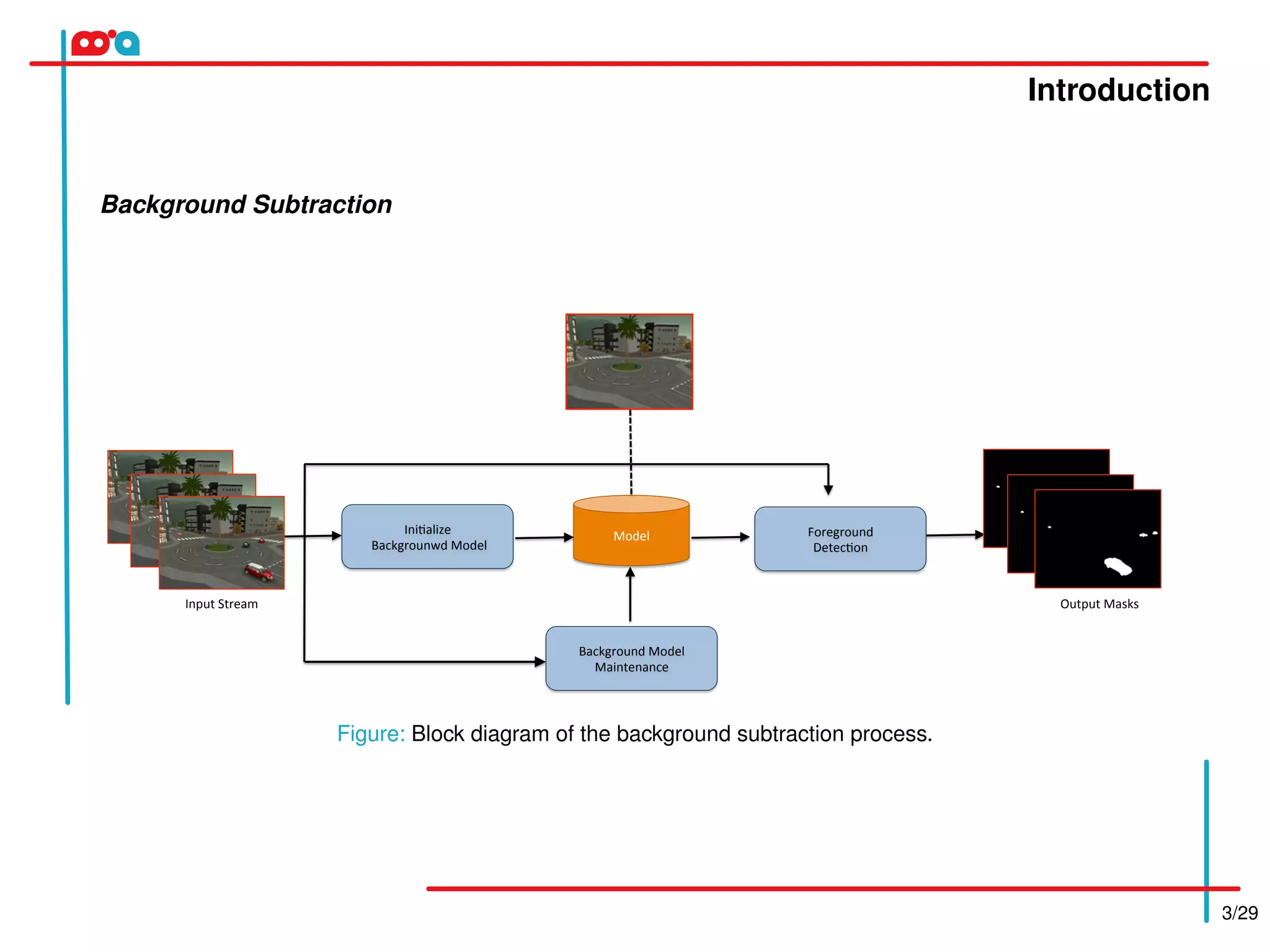
How to Choose the Classifier?
Bicego and Figueiredo, 2009 proposed a Weighted version that allow to use weights W = {w1,...,wN } in [0,1]
for the data.
R
R
R
a
wiξi
target
outlier
xi
Weighted One-Class SVM (WOC-SVM)
Minimizing the hypersphere volume implies the
minimization of R2
. To prevent the classifier from
over-fitting with noisy data, slack variables ξi are
introduced to allow some target points (respectively
outliers) outside (respectively inside) the hypersphere.
Therefore the problem is to minimize:
Θ(a,R) = R2
+C
N
∑
i=1
wi ξi (1)
where C is a user-defined parameter that controls the
trade-off between the volume and the number of
target points rejected. The larger C, the less outliers
in the hypersphere.
The BS task requires adjust the learned model to the scene variations over time](https://image.slidesharecdn.com/presentationicpr-170608133851/75/ICPR-2016-11-2048.jpg)

![Proposed Work
13/29
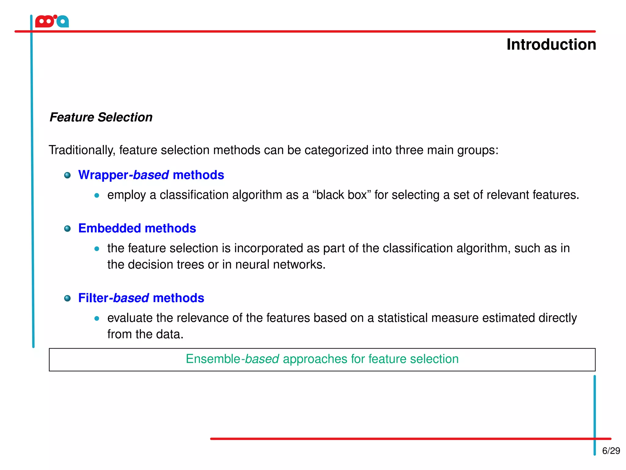
An Incremental Weighted One-Class SVM (IWOC-SVM)
We propose an IWOC-SVM which is closely related to the procedure proposed by Tax and Laskov (2003).
Given new samples Z1 = {x1,x2,...,xs} and its
respective weights not learned by the IWOC-SVM.
Karush-Kuhn-Tucker (KKT) conditions:
αi = 0 ⇒ ||xi −a||2
< R2
(2)
0 < αi < C ⇒ ||xi −a||2
= R2
(3)
αi = C ⇒ ||xi −a||2
> R2
(4)
The mathematical model can be defined as:
R −θ ≤ ||x −a||≤ R (5)
where θ ∈ [0,R] is relative to the distribution of
previous training set.
R
R
R
a
wiξi
target
outlier
xi
Algorithm 2 Incremental Weighted One-Class SVM
1: Require: Previous training set Z0, newly added training set Z1 and its respective weights
2: Train IWOC-SVM classifier on Z0, then split Z0 = SV0 ∪NSV0
3: Input new samples Z1. Put samples that violate KKT conditions in ZV
1 . If ZV
1 = /0, then goto 2.
4: Put samples from NSV0 that satisfy Eq. (5) into NSVS
0 .
5: Set Z0 = SV0 ∪NSVS
0 ∪ZV
1 and train IWOC-SVM classifier on Z0.
6: Output: IWOC-SVM classifier Ω and the new training set Z0.
.](https://image.slidesharecdn.com/presentationicpr-170608133851/75/ICPR-2016-13-2048.jpg)


![Proposed Work
17/29
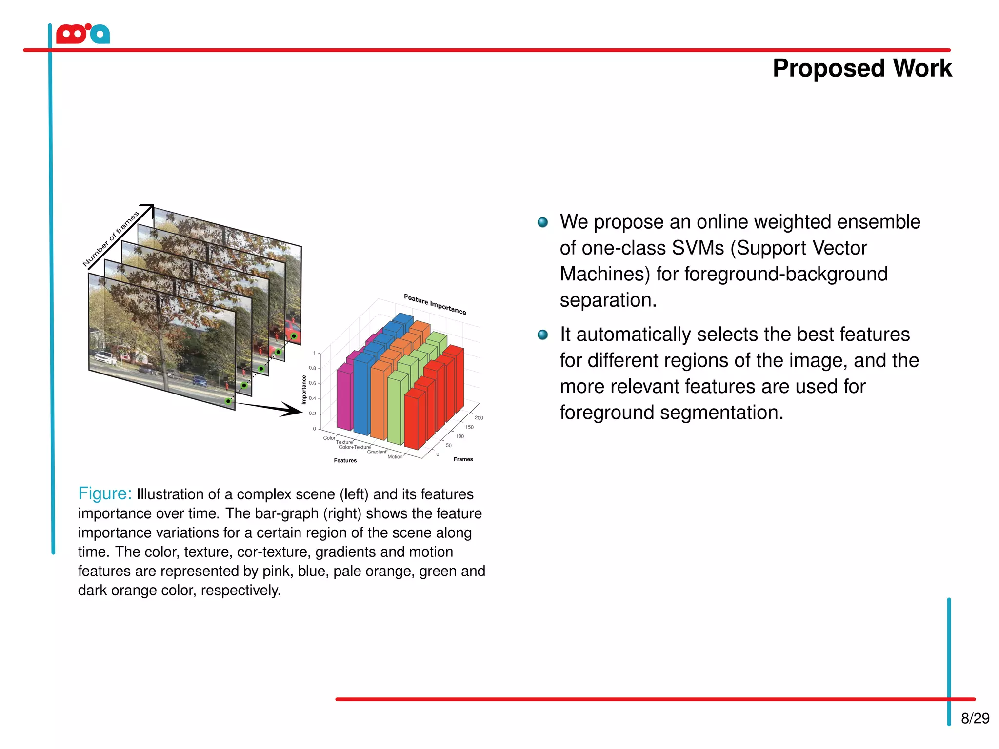
D. Heuristic approach for Background Model Maintenance
The Small Votes Instance Selection (SVIS) introduced by Guo and Boukir (Guo and Boukir, 2015) consists of an
unsupervised ensemble margin that combines the first c(1) and second most voted class c(2) labels under the
learned model. Let vc(1)
and vc(2)
denote the relative number of votes. Then the margin, taking value in [0,1] is:
m(x) =
vc(1)
−vc(2)
L
(10)
where L represents the number of best base classifiers in the ensemble. The first smallest margin instances are
selected as support vector candidates. The strong model is updated by the first smallest margin instances. This
procedure is presented in the Algorithm 4.
This heuristic significantly reduces the IWOC-SVM training task complexity while maintaining the accuracy of the
IWOC-SVM classification.](https://image.slidesharecdn.com/presentationicpr-170608133851/75/ICPR-2016-17-2048.jpg)


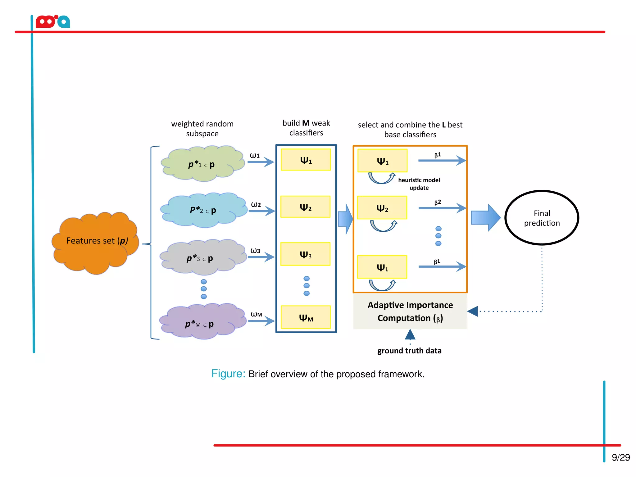
The proposed method uses an online weighted ensemble of one-class SVMs for feature selection in background/foreground separation. It automatically selects the best features for different image regions. Multiple base classifiers are generated using weighted random subspaces. The best base classifiers are selected and combined based on error rates. Feature importance is computed adaptively based on classifier responses. The background model is updated incrementally using a heuristic approach. Experimental results on the MSVS dataset show the proposed method achieves higher precision, recall, and F-score than other methods compared.