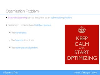
The document discusses machine learning optimization problems and linear/logistic regression algorithms. It notes that machine learning can be viewed as an optimization problem with constraints, a function to optimize, and an optimization algorithm. Linear regression aims to minimize prediction error by finding the best fitting linear model, while logistic regression predicts class probabilities using a sigmoid function. Both use gradient descent to optimize their error functions and learn model parameters from data.

![www.data4sci.com
@bgoncalves
Linear Regression
• We are assuming that our functional dependence is of the form:
• In other words, at each step, our hypothesis is:
and it imposes a Constraint on the solutions that can be found.
• We quantify our far our hypothesis is from the correct value using
an Error Function:
or, vectorially:
Sample 1
Sample 2
Sample 3
Sample 4
Sample 5
Sample 6
.
Sample M
Feature
1
Feature
3
Feature
2
…
value
Feature
N
X y
f ( ⃗
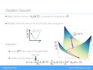
x ) = w0 + w1x1 + ⋯ + wnxn ≡ X ⃗
w
Jw (X, ⃗
y ) =
1
2m ∑
i
[hw (x(i)
) − y(i)
]
2
Jw (X, ⃗
y ) =
1
2m
[X ⃗
w − ⃗
y ]
2
hw (X) = X ⃗
w ≡ ̂
y](https://image.slidesharecdn.com/ppt-deeplearningfromscratch-230421101505-71983010/85/ppt-Deep-Learning-From-Scratch-pdf-3-320.jpg)

![www.data4sci.com
@bgoncalves
0
3.25
6.5
9.75
13
0 5 10 15 20
Geometric Interpretation
Quadratic error
means that an error
twice as large is
penalized four times
as much.
Jw (X, ⃗
y ) =
1
2m
[X ⃗
w − ⃗
y ]
2](https://image.slidesharecdn.com/ppt-deeplearningfromscratch-230421101505-71983010/85/ppt-Deep-Learning-From-Scratch-pdf-5-320.jpg)


![@bgoncalves
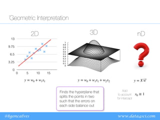
Logistic Regression (Classification)
• Not actually regression, but rather Classification
• Predict the probability of instance belonging to the given class:
• Use sigmoid/logistic function to map weighted inputs to
hw (X) ∈ [0,1]
hw (X) = ϕ (X ⃗
w)
[0,1]
z encapsulates all
the parameters and
input values
1 - part of the class
0 - otherwise](https://image.slidesharecdn.com/ppt-deeplearningfromscratch-230421101505-71983010/85/ppt-Deep-Learning-From-Scratch-pdf-12-320.jpg)

![www.data4sci.com
@bgoncalves
Logistic Regression
• Error Function - Cross Entropy
measures the “distance” between two probability distributions
• Effectively treating the labels as probabilities (an instance with label=1 has Probability 1 of
belonging to the class).
• Gradient - same as Logistic Regression
Jw (X, ⃗
y ) = −
1
m [yT
log (hw (X)) + (1 − y)
T
log (1 − hw (X))]
hw (X) =
1
1 + e−X ⃗
w
wj = wj − α
δ
δwj
Jw (X, ⃗
y )
δ
δwj
Jw (X, ⃗
y ) =
1
m
XT
⋅ (hw (X) − ⃗
y )](https://image.slidesharecdn.com/ppt-deeplearningfromscratch-230421101505-71983010/85/ppt-Deep-Learning-From-Scratch-pdf-14-320.jpg)


![www.data4sci.com
@bgoncalves
Comparison
• Linear Regression • Logistic Regression
δ
δwj
Jw (X, ⃗
y ) =
1
m
XT
⋅ (hw (X) − ⃗
y )
δ
δwj
Jw (X, ⃗
y ) =
1
m
XT
⋅ (hw (X) − ⃗
y )
Jw (X, ⃗
y ) = −
1
m [yT
log (hw (X)) + (1 − y)
T
log (1 − hw (X))]
Jw (X, ⃗
y ) =
1
2m
[hw (X) − ⃗
y ]
2
hw (X) = ϕ (Z)
hw (X) = ϕ (Z)
z = X ⃗
w z = X ⃗
w
ϕ (Z) =
1
1 + e−Z
ϕ (Z) = Z
Map features to a
continuous variable
Predict based on
continuous variable
Compare
prediction with
reality](https://image.slidesharecdn.com/ppt-deeplearningfromscratch-230421101505-71983010/85/ppt-Deep-Learning-From-Scratch-pdf-21-320.jpg)


![www.data4sci.com
@bgoncalves
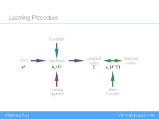
A practical example - MNIST
784 50 10 1
5000
examples
10 ⇥ 51
50 ⇥ 785
def predict(Theta1, Theta2, X):
h1 = forward(Theta1, X, sigmoid)
h2 = forward(Theta2, h1, sigmoid)
return np.argmax(h2, 1)
50 ⇥ 784 10 ⇥ 50
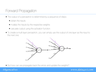
Forward Propagation
Backward Propagation
Vectors
Matrices
Matrices
X ⇥1 ⇥2
arg
max
def forward(Theta, X, active):
N = X.shape[0]
# Add the bias column
X_ = np.concatenate((np.ones((N, 1)), X), 1)
# Multiply by the weights
z = np.dot(X_, Theta.T)
# Apply the activation function
a = active(z)
return a](https://image.slidesharecdn.com/ppt-deeplearningfromscratch-230421101505-71983010/85/ppt-Deep-Learning-From-Scratch-pdf-43-320.jpg)


![[DSC Europe 25] Elena Menshikova - AI-Powered Operational Excellence: Revolut...](https://cdn.slidesharecdn.com/ss_thumbnails/es6nholbqy3zaao2c2yd-2-elena-menshikova-data-ai-in-decision-making-260115093812-4fba8b38-thumbnail.jpg?width=640&height=640&fit=bounds)


![[DSC Europe 25] Danilo Djukanovic - From Vibes to KPIs: Turning Culture Into ...](https://cdn.slidesharecdn.com/ss_thumbnails/inqestws5wf0cik2glgv-3-danilo-djukanovic-from-vibes-to-kpis-presentation-260114111931-dacff81f-thumbnail.jpg?width=640&height=640&fit=bounds)

![[DSC Europe 25] Nikola Vasiljevic - Player segmentation by combat playstyles ...](https://cdn.slidesharecdn.com/ss_thumbnails/mnvbf0yvrwaqsipzrrv3-2-nikola-vasiljevic-player-segmentation-by-playstyles-in-action-shooter-games-260114111931-b4d766cd-thumbnail.jpg?width=640&height=640&fit=bounds)


![[DSC Europe 25] Slobodan Dolinic - Smart and Intelligent Green Region.pptx](https://cdn.slidesharecdn.com/ss_thumbnails/0bribinjsp6ghwtvsvor-2-sigre-slobodan-dolinic-260115093812-c9c10e90-thumbnail.jpg?width=640&height=640&fit=bounds)
