This paper evaluates the effectiveness of second and fourth-order finite difference operators for solving time-dependent reaction-diffusion problems, highlighting why fourth-order methods are preferred. It discusses the method of lines for discretizing spatial derivatives in partial differential equations, leading to a system of ordinary differential equations in time. The paper also analyzes accuracy, stability, and convergence of these methods, providing computational experiments that demonstrate the superiority of fourth-order approximations over second-order ones.

1. Second or fourth-order finite difference operators, which one is most effective?
IJSM
Second or fourth-order finite difference operators, which one is most effective? Kolade M. Owolabi Department of Mathematical Sciences, Federal University of Technology, Akure, P.O. Box 704, Ondo State, Nigeria. Email: mkowolax@yahoo.com This paper presents higher-order finite difference (FD) formulas for the spatial approximation of the time-dependent reaction-diffusion problems with a clear justification through examples, “why fourth-order FD formula is preferred to its second-order counterpart” that has been widely used in literature. As a consequence, methods for the solution of initial and boundary value PDEs, such as the method of lines (MOL), is of broad interest in science and engineering. This procedure begins with discretizing the spatial derivatives in the PDE with algebraic approximations. The key idea of MOL is to replace the spatial derivatives in the PDE with the algebraic approximations. Once this procedure is done, the spatial derivatives are no longer stated explicitly in terms of the spatial independent variables. In other words, only one independent variable is remaining, the resulting semi-discrete problem has now become a system of coupled ordinary differential equations (ODEs) in time. Thus, we can apply any integration algorithm for the initial value ODEs to compute an approximate numerical solution to the PDE. Analysis of the basic properties of these schemes such as the order of accuracy, convergence, consistency, stability and symmetry are well examined. 2010 Mathematics Subject Classification: {92B05, 92C15, 35K55, 65M20, 76R50} Keywords: Consistency, finite difference, PDES, reaction-diffusion, stability, symmetry. INTRODUCTION Reaction-diffusion equations are classified as a special class of parabolic time-dependent partial differential equations. The major way of solving the class of these equations is through discretization. A well-known approach to solve time-dependent partial differential equation, with solutions varying in both time and space, is the method of lines (MOL), see Ascher et al. (1995), Schisser and Griffits (2009), Holden and Karlsen (2012) and Strikwerda (2004) for details. Application of this method requires to first constructing a semi-discrete approximation to the problem by setting up a regular grid in space, this is achieved by discretising the spatial independent variables with boundary constraints. Hence, a couple systems of ordinary differential equations are generated in time, which is associated with the initial value. Once that is done, we numerically approximate the solutions to the original time- dependent partial differential equation by marching forward in time on this grid. Conveniently, we can now apply any existing, and generally well established, time-stepping numerical methods such as the implicit-explicit (IMEX) schemes, Runge-Kutta methods or exponential time differencing (ETD) schemes among many others. In this paper, for the spatial discretisation, we are primarily concerned with the use of higher-order finite difference method. The discrete approximation to the derivatives will be converted into Toeplitz matrices. The discretisation in time uses majorly the exponential time differencing schemes, other time-stepping methods include but not limited to the fourth-order Runge-Kutta (RK4) method and implicit-explicit schemes. A brief of each of these methods will be International Journal of Statistics and Mathematics Vol. 1(3), pp. 044-054, August, 2014. © www.premierpublishers.org, ISSN: xxxx-xxxx x
Review

2. Second or fourth-order finite difference operators, which one is most effective?
Owolabi 044
discussed later in this paper. In the title l propose second or fourth-order operators which one is more effective?
Once computational experiments are conducted, there are some important issues such as consistency, stability and
convergence that are required to be investigated, once these issues as pointed out are addressed, the question
posed by the title of this paper is answered. We can now proceed to solve numerically the class of reaction-diffusion
problems to be considered.
The rest of this paper is structured into 5 sections. Higher order finite difference approximations are discussed in
Section 2. Section 3 gives a detail report on error analysis and order of accuracy of the schemes. Stability analysis,
convergence and symmetric properties are presented in Section 4 with numerical results on reaction-diffusion
problems. Conclusions are drawn in Section 5.
Finite Difference Approximations
The finite difference methods have gained its dominance in the various fields of computational science since its
inception as the major method of choice back to 1960s. Other methods such as finite element and boundary element
methods enjoyed recent popularity, finite difference methods are still well utilized for a wide array of computational
engineering and science problems.
A finite difference scheme is produced when the partial derivatives in the partial differential equation(s) governing a
physical phenomenon are replaced by a finite difference approximation. The result is a single algebraic equation or a
system of algebraic equations which, when solved, provide an approximation to the solution of the original partial
differential equation at selected points of a solution grid. The solution grid (also referred to as computational grid or
numerical grid) is originated by dividing the axes representing the independent variables in the solution domain into
a number of intervals. The two extreme points of the interval are replaced by the boundary conditions in the given
problem. If we draw lines perpendicular to a given axes passing through the extreme points of the intervals, the
resulting grid is the computational grid.
Higher order finite difference approximations
Higher order finite difference approximations can be obtained by taking more terms in Taylor series expansion. The
Taylor expansion provides a very useful tool for the derivation of higher order approximation to derivatives of any
order. Our interest in this work is to use higher order finite difference formula for the spatial discretization of the
problems to be considered later in this work, so we need to create an estimate based on step size 2x through the
Taylor series expansion




  
0
( ) ( )
!
(2 )
( 2 )
k
j
k
k
j u x
k
x
u x x (2.1)




   
0
( ) ( )
!
(2 )
( 2 ) ( 1)
k
j
k
k
k
j u x
k
x
u x x (2.2)
Better approximation is obtained by combining these two estimates through the process called Richardson
extrapolation. For instance, we present the fourth-order centred finite difference schemes for the first and second
derivatives as
( )
12
( 2 ) 8 ( ) 8 ( ) ( 2 )
( ) 4 x
x
u x x u x x u x x u x x
u x j j j j
j  

          
  (2.3)
and
( )
12
( 2 ) 16 ( ) 30( ) 16 ( ) ( 2 )
( ) 4
2 x
x
u x x u x x x u x x u x x
u x j j j j j
j  

            
  (2.4)
respectively. For the purpose of comparison, we present the conventional second order FD scheme as
( )
( ) 2 ( ) ( )
( ) 2
2 x
x
u x x u x u x x
u x j j j
j  

     
  (2.5)
Some of the important features to notice about centred finite difference schemes, they are symmetric in nature and
posses an even-order of accuracy. The weights of some of the central finite difference formulas are presented in the
Tables 1 and 2 for the approximations of first and second derivatives respectively.

3. Second or fourth-order finite difference operators, which one is most effective?
Int. J. Stat. Math. 045
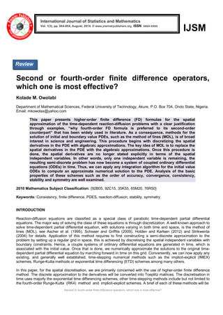
Table 1. Weights of some higher order centered finite difference approximation for the first derivatives on
equi-spaced grids
Order of
accuracy
4 u 3 u 2 u 1 u 0 u 1 u 2 u 3 u 4 u
2
2
1

0
2
1
4
12
1
-
12
8
0
12
8
-
12
1
6
60
1

60
9
60
45

0
60
45
60
9

60
1
8
840
3
840
32

840
168
840
672

0
840
672
840
168

840
32
840
3

Table 2. Weights of some higher order centered finite difference approximation for the second derivatives on equi-spaced
grids
Order of
accuracy
4 u 3 u 2 u 1 u 0 u 1 u 2 u 3 u 4 u
2 1 -2 1
4
12
1

12
16
12
30

12
16
12
1

6
180
2
180
27

180
270
180
490

180
27
180
27

180
3
8
560
1

315
8
5
1

5
8
72
205

5
8
5
1

315
8
560
1

where i u for i 1,2,3,4 has the equivalence ( 4 ), , ( 4 ) 4 4 u u x x u x x j j        in the tables. In general,
schemes for any given derivatives of any chosen order can be derived from Taylor expansions as long as sufficient
number of sample points is used. These approximations are much more difficult far beyond the simple cases shown,
most especially, the higher order formulas. Readers are referred to the books by Fornberg (1995, 1998), Fornberg
and Driscoll (1999) where schematic illustration of how to generate the weights of higher order centered and one-side
finite differences formulas for approximating derivatives up to fourth-order equi-spaced grids with order of
accuracy up to eighth can be found.
For more general finite difference approximations, we follow the description given by Fornberg (2011) and present
briefly the short code that can be used to generate weights of any order approximation schemes on equi-spaced
grids. The program only requires Mathematica package (version seven and above) that contains pre-loaded Pade’
package. The complete code is
t=PadeApproximation[xs(Log[x]/h )m ,{x,1,{n,d}} ];
CoefficientList[{Denominator[t],Numerator[t]},x ]
The numbers d, m, n and s describe the shape of the stencil, where d is the number of grid intervals in between the
left- and right most derivative entries, m indicates the number of
derivatives to be approximated, n stands for the number of grid intervals in between the left- and rightmost function
entries, and s the number of grid intervals in between the leftmost derivative and function entries.
Error Analyses
Next, we need to ask ourselves why using fourth-order approximation scheme instead of the commonly used
second-order scheme approximation? To answer this question, let us quickly consider an example (Mathews and

4. Second or fourth-order finite difference operators, which one is most effective?
Owolabi 046
Fink 1999). Givenu(x)  cos(x) , we use formulas (2.5) and (2.4) with x  0.1,0.01 and 0.001to find
approximations tou(0.8) . The true value here is taken to be u(0.8)  cos(0.8) . For instance, the calculation for
x  0.01 with methods (2.5) is
0.696690000
0.0001
(0.81) 2 (0.80) (0.79)
(0.8)  
 
 
u u u
u .
By subtracting the computed value from the true value, we found the error in this approximation to be 1.0671e-005.
The remaining calculations are summarized in the Table 3
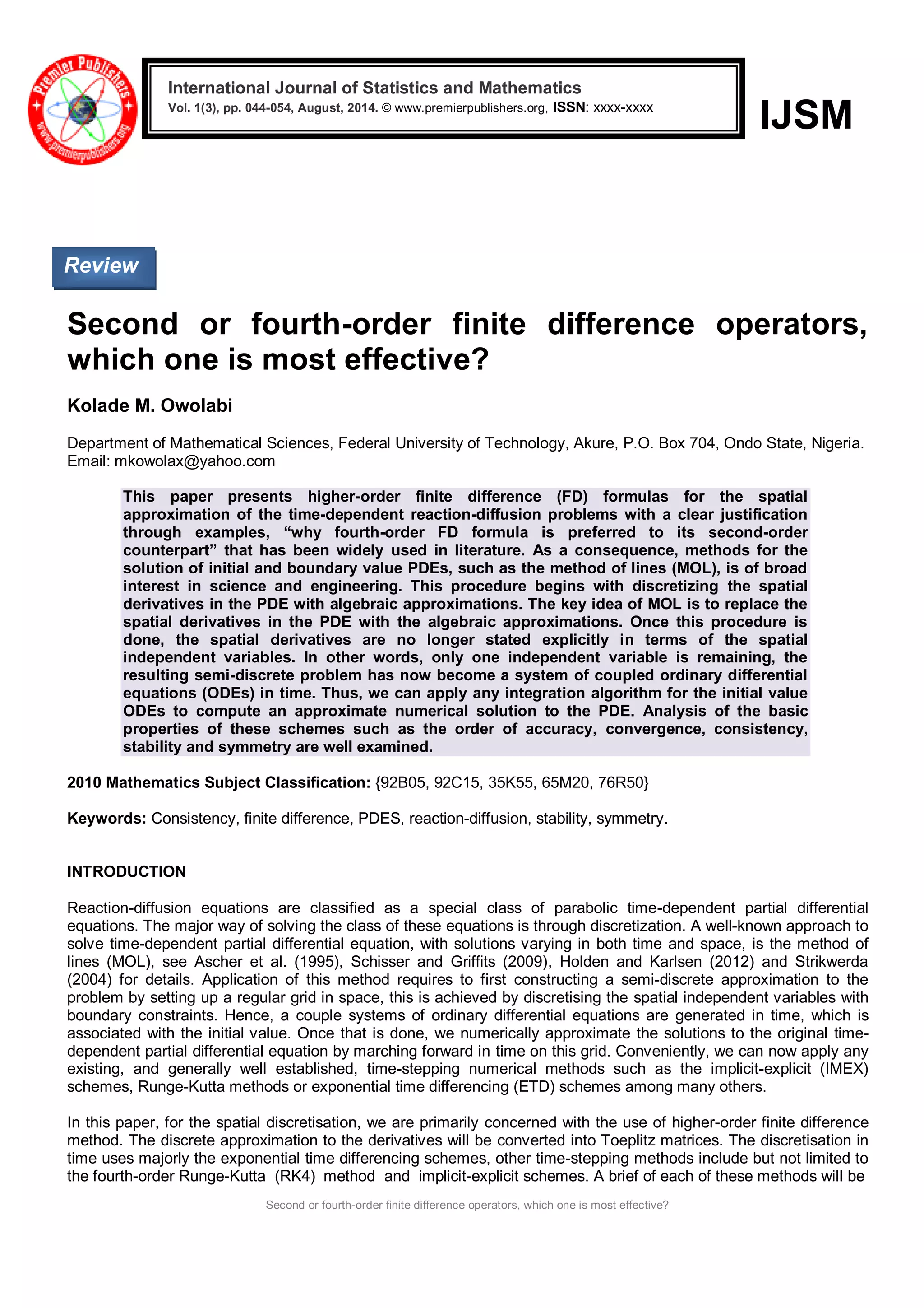
Table3: Numerical approximation using the second-order
formula (2.5)
Step size (x) Approximation Error
x 1.0 -0.640548935 -0.056157774
x  0.1 -0.696126300 -0.000580409
x  0.01 -0.696600000 -0.000016709
x  0.001 -0.696000000 -0.000706709
In the same manner, for the fourth-order formula, we obtain
Table 4. Numerical approximation using the fourth-order
formula (2.4)
Step size (x) Approximation Error
x 1.0 -0.689625413 -0.007081296
x  0.1 -0.696705958 -0.000000751
x  0.01 -0.696000000 -0.000016709
x  0.001 -0.696750000 -0.000031709
The results obtained in the Tables 3 and 4 have shown that the fourth-order scheme produces a better
approximation when compared to its second-order counterpart. The optimal step-size for the formula (2.5) is at when
x  0.01 as shown in Table 3 and the optimal step-size to be used for equation (2.4) is whenx  0.1. We can
see here that the fourth-order allows large step-size.
Next, we analyze briefly the two approximation methods of orders ( ) 2  x and ( ) 4  x that are paramount to our
discussion in this paper. Let k k k u   , where k  is the error in computing ( ) k u x , then (2.5) can be written in
the form
( , )
( ) 2 ( ) ( )
( ) 2 E u x
x
u x x u x u x x
u x  

     
  . (3.6)
The error term E(u,x) consists of both the truncation and the round-off errors. That is,
12
( ) 2 ( ) ( ) ( )
( , ) ( , ) ( , )
2 (4)
2
x u c
x
x x x x x
E u x E u x E u x round trunc



     

    
   (3.7)
where | ( ) | (4) u c is assumed to be bounded for c  c(x)[x  x, x  x], then the truncation error in (3.7) goes
to zero in the same manner with ( ) 2  x . Since one can assume that each error k  has magnitude , and that
| ( ) | (4) u x  M , then we can obtain the error bound, if | | k and max[ , ]{ ( )} (4) M  x  x x  x u x , then
| ( , ) | 4 / /12 2 2 E u x   x Mx . On simplifying further, the optimum step size is obtained as
1/ 4 x  (48 /M) and that | ( ) | cos( ) 1 (4) M  u x  x  .
Int. J. Stat. Math. 047

5. Second or fourth-order finite difference operators, which one is most effective?
It is clear that the portion of the error due to round off is inversely proportional to the square of x , this particular
term grows when x gets small, and it is referred to as the step-size dilemma in most cases. The only way out of
this problem is to use a higher order method that would accommodate a larger value of x to yield the desired
accuracy. This assertion actually prompts us to seek higher order approximation method. Similarly, we define the
bound for the error term in (2.4) as | ( , ) | 16 /3 /90 2 4 E u x   x Mx with an optimal step size value given as
1/ 6 x  (240 /M) , in such that | ( ) | cos( ) 1 (6) M  u x  x  . Convergence of the second- and fourth-order finite
difference approximations are shown in Tables 1 and 2 respectively.
Figure 1. Second-order convergence of the finite difference (2.5). The
use of Toeplitz matrices permits high values of N.
Figure 2. Fourth-order convergence of the finite difference (2.4). The use
of Toeplitz matrices permits high values of N.
Illustrative Example
Most physical applications encountered in the various fields of science and engineering are described in term of
dimensions (space and time). Most mathematical description exists in terms of partial differential equations
Owolabi 048
10
0
10
1
10
2
10
3
10
4
10
-8
10
-7
10
-6
10
-5
10
-4
10
-3
10
-2
10
-1
10
0
N
Error
Convergence of second-order finite differences
10
0
10
1
10
2
10
3
10
4
10
-15
10
-10
10
-5
10
0
N
Error
Convergence of fourth-order finite differences

6. Second or fourth-order finite difference operators, which one is most effective?
explaining the concept of physical space-time. As a result of this fact, methods for the solution of partial differential
equations, such as the method of lines by Hamdi et al. (2010) and Strikwerda (2004) are still active in the current
field of research. As a basic illustrative example of a PDE, let us consider the diffusion equation
, 0 2
2






t
x
u
D
t
u
(3.8)
where u(x, t) is the population density in biological or ecological processes or the concentration in the chemical or
physical contexts. D is regarded as the diffusion. Equation (3.8) also governs unsteady heat transfer in a solid
medium and one-dimensional Stokes flow.
Solution of equation of the form (3.8) is subjected to some auxiliary conditions that can be determined by the
highest order of the derivatives in each of the independent variables present (see Powers (2006), Meyer (1973),
Kreiss and Lorenz (1989)). To illustrate the method of lines procedure to solve diffusion equation (3.8), suppose that
u(x, t) is discretized in space with N 1points, of which N 1are the interior points, on a uniform grid with step
size x , we have
u x t u t j N j j ( , )  ( ), 0   , (3.9)
where the index j indicating a position along the grid in x and x is the spacing in x along the grid, assumed to be
constant. To find an algebraic approximation to the spatial
derivative 2 2  u / x in (3.8). For instance, the fourth-order centered finite difference approximation, yields the
following ODEs
 
]
12
( ) 16 ( ) 30 ( ) 16 ( ) ( )
[
( )
( ),
2
1 4 3 2 1 0
0
x
u t u t u t u t u t
D
dt
du t
u f t a

    


( ) ( ),
]
12
( ) 16 ( ) 30 ( ) 16 ( ) ( )
[
( )
2
1 1 2 3 4
u t f t
x
u t u t u t u t u t
D
dt
du t
N N
N N N N N N


    
     
(3.10)
subject to the initial condition
( , 0) ( ), 0 , 0 u x t u x j N j j     (3.11)
where f (t) a and f (t) N are the left and right boundaries of u for all t. Equations (3.10) and (3.11) constitute the
complete MOL approximations of (3.8).
Order of Accuracy and Consistency
With the second order schemes and by means of the Taylors expansion, Eq. (3.8) becomes
( ) ( ).
( , )
320
( , )
6
( , )
24
( , )
2
( , ) ( , )
( , ) ( , ) ( , ) 2 ( , ) ( , )
2
0 0
4
0 0
2
0 0
2
0 0
2
0 0 0 0
2
0 0 0 0 0 0 0 0 0 0
t x
u x t
x
u x t D
t
u x t
x
u x t D
t
u x t D u x t
x
u x x t u x t u x x t
D
t
u x t t u x t
ttt xxxxxx
tt xxxx
t xx
     
 

 




 

 
   

     


  

(3.12)
The right hand side of (3.12) is the so-called truncation error, and the lowest powers of t and x in the truncation
error are the respective order of accuracies of the finite difference approximations in time and space. Thus, the finite
difference scheme in (3.12) is consistent with the diffusion equation (3.8) to first-order accuracy in time and second-order
accuracy in space.
In the same way, when fourth-order schemes are applied to (3.8), we obtain
Int. J. Stat. Math. 049

7. Second or fourth-order finite difference operators, which one is most effective?
 

 


   

            

           
( , )
90
( , )
30
( , ) ( , )
12
( 2 , ) 16 ( , ) 30 ( , ) 16 ( , ) ( 2 , )
12
( , 2 ) 8 ( , ) 8 ( , ) ( , 2 )
0 0
4
0 0
4
0 0 0 0
2
0 0 0 0 0 0 0 0 0 0
0 0 0 0 0 0 0 0
u x t
x
u x t D
t
u x t D u x t
x
u x x t u x x t u x t u x x t u x x t
D
t
u x t t u x t t u x t t u x t t
ttttt xxxxxx
t xx
(3.13)
The truncation error is defined as n
j n j
n
j T  u(x , t )  u . Hence, 4
2
4
1 | T | t x n
j       , where 1  and 2  denote
two constants that depend on some norms of the derivatives of u. As a result, this scheme is consistent with order
of accuracy 4 in both space and time. Generally, if the truncation error is ( , ) p q  x t , the method is th p order
accurate in x and th q order accurate in t . If the truncation error tends to zero as x,t 0 , the scheme is said to
be consistent.
A finite difference scheme is convergent to th p order in x and th q in t if
N H
j
H
H j
u u x
1
1
| |  


 


  
,
where H  2 corresponds to the Euclidean norm and H   is the maximum norm. By Lax Equivalence Theorem
(Lax and Richtmyer 1956), the importance of the concepts of consistency and stability is seen in the Lax-Richtmyer
equivalence theorem, which is the fundamental theorem in the theory of finite difference schemes for initial value
problem. It states that, if a finite difference method for a given partial differential equation for which initial value
problem is well-posed and that the scheme is linear, stable and accurate of order ( , ) p q  x t , it is convergent.
Definition of Illustrative Example
A numerical scheme that is symmetric is consistent (see Fatunla (1988), Lambert and Watson (1976) ) if
(i) it has order ( p,q) 1.
(ii) the sum of its first characteristic polynomial is zero., that is
 

0
0
j j  .
Hence the schemes are consistent.
The matrix notation
The easiest way of representing the approximation to the differential operator is by the use of the differentiation
matrix, Trefethen (1996, 2000). The matrix operator forms a Toeplitz matrix in which the order of the approximation
determines the sparsity of the matrix.
Definition Order of Accuracy and Consistency
A Toeplitz matrix, is a matrix in which each ascending diagonal from left to right has constant entries, that is, a matrix
of the form
 





 






  


1 2 1 0
1
1 0 1
0 1 2 1
l l l l
l
l l l
l l l l
L
N
N

   
 

(3.14)
where the entries of L satisfy the property ij j i l l   , then L is said to be a circulant matrix with eigenvalues given
by



N
j
N
n
i j
n jl e
1
2 ( 1)
,

 for n  0,1,,N 1.
Owolabi 050

8. Second or fourth-order finite difference operators, which one is most effective?
Considering the sequence
s {l : k p, , 1,0, ,q} k      ,
where p and q are positive integers. A square Toeplitz matrix L of order N is of the bandwidth (p  q 1)  N , if
its entry ij l is a member of the sequence s and zero otherwise. For instance, if p  q  2, then L is a pentdiagonal
Toeplitz matrix.
The present paper is primarily concerned with the eigenvalues of Toeplitz matrices obtained from the finite difference
schemes. It will also be of paramount importance for determining the linear stability of our problems. The
eigenvalues of a tridiagonal Toeplitz matrix of arbitrary order N are well understood Mitchell (1980). The major
challenge rest upon the Toeplitz matrix with higher bandwidth, the eigenvalue problems become intractable, see for
instance the work of Sogabe (2004, 2008), although some algorithms have been derived for pentdiagonal matrices,
see Cinkir (2012), Hoffman (2001), Leveque (2007), Durran (2010), Kilic and El-Milkkawy (2008) and El-Milkkawy
(2004) for details. An attempt to circumvent the difficulty in finding the eigenvalues of higher bandwidth Toeplitz
matrices, we shall concentrate basically on the eigenvalues of the circulant Toeplitz matrices, which is more
importantly related to our assumption of periodic boundary conditions.
Stability Analysis
Let us consider the parabolic partial differential equation with one spatial independent variable
(1 )
2
2

 
u
u
x
u
t
u
 





, (4.15)
known as the Fisher equation, where , and  are positive parameters. Using second order schemes, the Von
Neumann’s stability of the Eq. (4.15 ) can be verified as
1
2
1 4 sin2  


 

k x m  ,
where m k is the wave number, 2   t x called the Courant number (Courant et al. (1967)) and we also let
   1, for simplicity. The maximum value of the sine function is considered so that 1 4  1 and   0 . For
  0 , it implies that t  0 , which is impractical. Thus, we have0  1/ 2 . In order to ensure a stable solution
or reduce errors, maximum care must be exercised in selecting the value of . It further implies that for a givenx ,
the allowed value of t must be small enough to satisfy 1/ 2 . We conclude by saying that a finite difference
equation is stable if it produces a bounded solution when the exact solution is bounded, and is unstable if it produces
an unbounded solution when the exact solution is bounded.
Similarly, when the fourth order scheme is applied to (4.15), we obtain the amplification polynomial
8 8 1 0 4 3 2    G     ,
where G  2cos2  32cos  3 . By Intermediate Value Theorem, we let
( ) 8 8 1 4 3 2 g     G    ,
which is a continuous function. We want to show that there exists a root  1 for g(x)  0 on [0, 1]. Observe
that g(0)  1 0and g(1)  G with possibility of cases (i) G  0 (ii) G  0and (iii) G  0 . It is
obvious that the method is stable if |G |1, so the scheme is conditionally stable.
Linear stability analysis can also be verified by setting  0, reaction-diffusion Eq.(4.15) reduces to a standard
diffusion equation (3.8) , its two level difference is presented as
, 0,1,2, 1
1
0     L u L u b n n n n (4.16)
where n b is expected to have contained the boundary conditions and | | 0 0 L  . For L  I 0 , the difference scheme
(4.16) is explicit otherwise it is an implicit method. In the stability analysis of the matrix method, we determine the
conditions under which the error norm
n n u Er  u  u 1
where . indicates the stable norm, is bounded as n. Again, we can rewrite (4.16) in the form
Int. J. Stat. Math. 051

9. Second or fourth-order finite difference operators, which one is most effective?
, 0,1,2, 1    Er Er n n n 
where 1
1
0 L L    and  is called the amplification matrix. With n=1, 2, ..., we have
1 0 1
Er Er
n n
n  
  .
Therefore, for the stability we require that   1 . In this paper, our particular case is when  is symmetric matrix,
then ( )
2
    in such a way that it equivalence form ( ) 1. Hence, von Neumann necessary condition is
satisfied.
Convergence
On applying the second order scheme to the diffusion equation (3.8) and let t k and xh , and expand
each terms in Taylors series, we obtain the truncation error formula
( )
2 12
2 12
( , ) ( , ) [ ( , ) 2 ( , ) ( , )]
4 2
2 2
4
4
2 2
2
2
1 1 1
u u k h
kh
u
k
u
h
h u
h
k
u
k
ku
E u x t u x t u x t u x t u x t
tt x
t tt x x
trunc j n j n j n j n j n
    






 


 


   


 


  
       


(4.17)
where u t t   /  and u x x   /  . The trunc E of the method is of order ( ) 2 2  k  kh . The order of the method is
given as
( ) ( )
1 2 E k h
k trunc    .
If the solution of the difference equation tends to the solution of the differential equation as h0 and k 0 , then
the difference equation is said to be convergent. The same process can be repeated for the fourth-order scheme.
Hence, we conclude with the definition of convergence.
Definition Convergence
Gedney (2011) that says; A finite difference equation (FDE) is consistent with a partial differential equation (PDE) if
the difference between the FDE and the PDE (i.e., the truncation error) vanishes as the sizes of the time step k or
t and spatial grid spacing h or x go to zero independently, is satisfied.
In addition, the Lax-Richtmyer (1956) equivalence theorem states that a consistent finite-difference scheme for a
partial differential equation for which the initial-value problem is well posed is convergent if and only if it is stable, for
a proof, readers are referred to Strikwerda (2004), Thomas(1995, 1999) and Sewel (1991). Finally, by Dahlquist
equivalence theorem, a linear multistep formula is convergent if and only if it is consistent and stable.
Symmetry
According to Fatunla (1988), Jain (1984) and Lambert and Watson (1976), the fourth-order schemes (2.3-2.4) is said
to be symmetric if when the values of s j   and s j   are interchanged, the function is the same or is multiplied by
minus one.
J J j J j j j j  ,  ,  0(1)       (4.18)
where j  and j  correspond to the coefficients of the first and second characteristic polynomial when applied to
(3.8). It follows that
0
8
1
2 2
1 3
0 4
  
   
   
 
 
 
and
30
16
1
2 2
1 3
0 4
 
  
  
 
 
 
Owolabi 052
Hence, the method is symmetric.

10. Second or fourth-order finite difference operators, which one is most effective?
Numerical results
Numerical method of solution discussed earlier is applied to solve both the diffusion equation (3.8) and the reaction-diffusion
equation (4.15), subject to the initial condition
, [ , ]
cosh( )
1
( ,0) x a b
x
u x  

(4.19)
and homogeneous Dirichlet boundary conditions
u(a, t)  u(b, t)  0, t  0 (4.20)
The choices of parameters a and b determines how well the waves propagate. When both equations (3.8) and (4.15)
are discretized in space with the fourth-order central difference scheme (2.4), it results to the ordinary differential
equations in time. The resulting ODEs is advanced with the MATLAB ode15s solver.
Figure 3. Solution of the reaction-diffusion equation (4.15) at parameters values
D  0.5,  1/ 2, t  0.001, N  200 for x[15,15] .
Int. J. Stat. Math. 053
-10
-5
0
5
10
0
0.5
1
x 10
-3
0.2
0.4
0.6
0.8
t x
u(x,t)

11. Second or fourth-order finite difference operators, which one is most effective?
Figure 4: Solution of the reaction-diffusion equation (4.15) at parameters values
D  0.05,  1/8,   5,  1, t  0.01, N  200 for x[15,15] .
Conclusions
To this end, we have dealt with spatial discretization method using finite difference (FD) schemes of higher orders. A
less rigorous method of derivation of higher-order FD schemes has been reported with the aid of a Mathematica
program that contains the pre-loaded Pad'e package, with a view of circumventing the difficulty associated with the
derivation of FD formula with order greater than two, see Tables 1 and 2 for details. Also in this paper, the question
of ``why using fourth-order FD schemes against the commonly used second-order scheme'' is well-answered. A
proof to this assertion is clearly shown in the results presented in Tables 3 and 4 for the second- and fourth-order FD
schemes respectively for different values of x . It is evident from the results presented that the fourth-order scheme
yields a better approximation in comparison to the second-order scheme, as it permits the use of higher step-size.
More importantly, the convergence test results presented in Figures 1 and 2 further justify the supremacy of fourth-order
scheme (2.4) over its second-order counterpart (2.5) by error factor of about 14 10 against 7 10 respectively.
Accuracy and suitability of our schemes was ascertained via the analysis of their basic properties such as order of
accuracy, consistency, convergence, stability and symmetry.
REFERENCES
Ascher UM, Ruth SJ, Wetton BTR, Implicit-explicit methods for time- dependent partial differential equations, SIAM
Journal on Numerical Analysis 32: 797-823.
Cinkir Z (2012). A fast elementary algorithm for computing the determinant of Toeplitz matrix. Numerical Analysis.
arXiv:1102.0453v2
Courant R, Friedrichs K, Lewy H (1967). On partial difference equations of mathematical physics. IBM Journal of
Research and Development. 11: 215-234.
Crank J, Nicolson E (1963). A practical method for numerical integration of solutions of partial differential equations
of heat-conduction type. Proceedings of the Cambridge Philosophical Society. 43: 50-67.
Owolabi 054
0
0.005
0.01
-15
-10
-5
0
5
10
15
0.3
0.4
0.5
0.6
0.7
0.8
0.9
x
t
u(x,t)

12. Second or fourth-order finite difference operators, which one is most effective?
Durran DR (2010). Numerical Methods for Fluids Dynamics with Applications to Geophysics. Springer Science+Business Media. New York. Fatunla SO (1988). Numerical Methods for IVPs in Ordinary Differential Equations, Academic. Press Inc. Harcourt Brace Jovanovich Publishers. New York. Fornberg B (1998). Calculation of weights in finite difference formulas. SIAM Review 40: 685-691. Fornberg B, Driscoll TA (1999). A fast spectral algorithm for nonlinear wave equations with linear dispersion. Journal of Computational Physics. 155: 456-467. Fornberg B (2011). Finite difference method. Scholarpedia 6 (10) 9685. Gedney SD (2011). Introduction to the Finite-Difference Time-Domain (FDTD)-Method for Electromagnetics. Morgan and Claypool Publishers, Arizona. S. Hamdi S, Schiesser WE, Griffiths GW (2010). Method of lines. Scholarpedia. 2(7):2859. Hoffman JD (2001). Numerical Methods for Engineers and Scientists, Marcel Dekker Inc. New York. Holden H, Karlsen KH (2012). Nonlinear Partial Differential Equations. The Abel symposium, Springer-Verlag Berlin Heidelberg. Jain RK (1984). Numerical solution of differential equations. Wiley Eastern limited, New Delhi. Kilic E, El-Milkkawy M(2008). A computational algorithm for special nth-order pentadiagonal Toeplitz determinants. Applied Mathematics and Computation. 199: 820-822. Kreiss N, Lorenz J (1989). Initial-Boundary Value Problems and the Navier-Stokes Equations. Academic Press, San Diego. Lambert JD, Watson A (1976). Symmetric multistep method for periodic initial value problem. Journal of the Institute of Mathematics and its Applications. 18: 189-202. Lax PD, Richtmyer RD (1956). Survey of the instability of linear finite difference equations. Communications on Pure and Applied Mathematics. 9: 267-293. Leveque RJ (2007). Finite Difference Methods for Ordinary and Partial Differential Equations. SIAM, Philadelphia. Mathews JH, Fink KD (1999). Numerical Methods Using MATLAB. Prentice Hall, New Jersey. Meyer GH (1973). Initial Value Methods for Boundary Value Problems-Theory and Application of Invariant Imbedding. Academic Press, New York. El-Mikkawy M (2004). A fast algorithm for evaluating nth order tri-diagonal determinants. Journal of Computational and Applied Mathematics. 166: 581-584. Mitchell AR, Griffiths DF (1980). The Finite Difference Method in Partial Differential Equations. John Willey and Sons Ltd. Powers DL (2006). Boundary value Problems and Partial Differential Equations. Elsevier Academic Press, USA. Sewell G (2005). The Numerical Solution of Ordinary and Partial Differential Equations. John Wiley and Sons, Inc., Hoboken, New Jersey. Schiesser WE (1991). Numerical Method of Lines Integration of Partial Differential Equations. Academic Press, San Diego. Schiesser WE, Griffiths GW (2009). A Compendium of Partial Differential Equation Models: Method of Lines Analysis with Matlab. Cambridge University Press, Cambridge. Strikwerda JC (2004) Partial Difference Schemes and Partial Differential Equations. SIAM, Philadelphia. Thomas JW (1995). Numerical Partial Differential Equations - Finite Difference Methods. Springer-Verlag, New York. Thomas JW (1999). Numerical Partial Differential Equations: Conservation laws and elliptic equations. Springer- Verlarg, New York. Trefethen LN (1996). Finite Difference and Spectral Methods for Ordinary and Partial Differential Equations. Upson Hall Cornell University Ithaca, New York. Trefethen LN (2000) Spectral Methods in MATLAB. SIAM, Philadelphia. Accepted 06 September, 2014. Citation: Owolabi KM (2014). Second or fourth-order finite difference operators, which one is most effective?. International Journal of Statistics and Mathematics, 1(1): 044-054. Copyright: © 2014 Owolabi KM. This is an open-access article distributed under the terms of the Creative Commons Attribution License, which permits unrestricted use, distribution, and reproduction in any medium, provided the original author and source are cited.