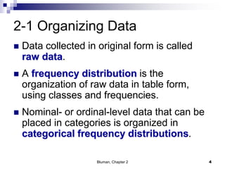
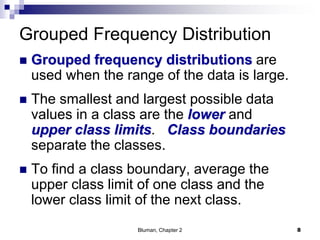
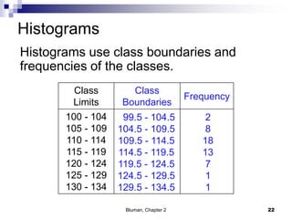
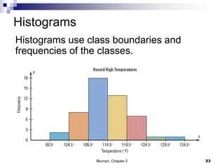
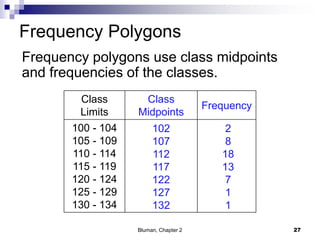
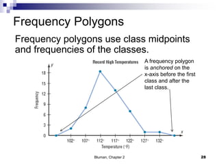
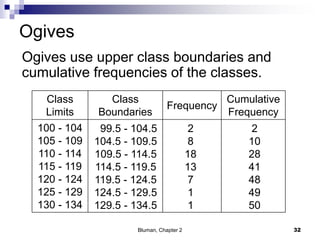
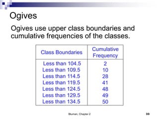
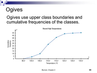
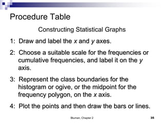
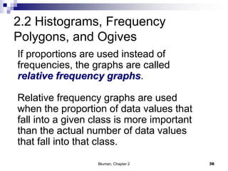
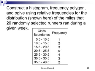
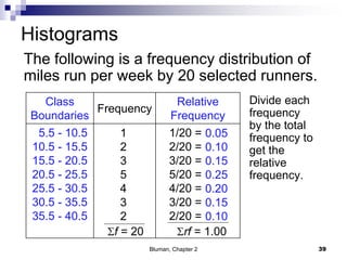
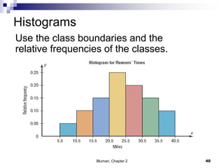
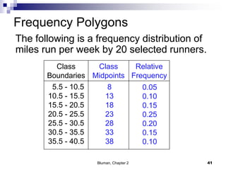
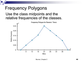
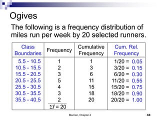
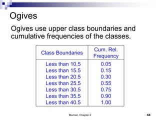
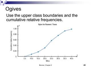
Chapter 2
Frequency Distributions
and Graphs
1
© McGraw-Hill, Bluman, 5th ed, Chapter
2
Chapter 2 Overview
Introduction
 2-1 Organizing Data
 2-2 Histograms, Frequency
Polygons, and Ogives
 2-3 Other Types of Graphs
 2-4 Paired Data and Scatter Plots
2Bluman, Chapter 2
Chapter 2 Objectives
1. Organize data using frequency distributions.
2. Represent data in frequency distributions
graphically using histograms, frequency
polygons, and ogives.
3. Represent data using Pareto charts, time
series graphs, and pie graphs.
4. Draw and interpret a stem and leaf plot.
5. Draw and interpret a scatter plot for a set of
paired data.
3Bluman, Chapter 2
2-1 Organizing Data
 Data collected in original form is called
raw data.
 A frequency distribution is the
organization of raw data in table form,
using classes and frequencies.
 Nominal- or ordinal-level data that can be
placed in categories is organized in
categorical frequency distributions.
4Bluman, Chapter 2
Chapter 2
Frequency Distributions and
Graphs
Section 2-1
Example 2-1
Page #38
5Bluman, Chapter 2
Categorical Frequency Distribution
Twenty-five army indicates were given a blood
test to determine their blood type.
Raw Data: A,B,B,AB,O O,O,B,AB,B
B,B,O,A,O A,O,O,O,AB AB,A,O,B,A
Construct a frequency distribution for the data.
6Bluman, Chapter 2
Categorical Frequency Distribution
Twenty-five army indicates were given a blood
test to determine their blood type.
Raw Data: A,B,B,AB,O O,O,B,AB,B
B,B,O,A,O A,O,O,O,AB AB,A,O,B,A
Class Tally Frequency Percent
A
B
O
AB
IIII
IIII II
IIII IIII
IIII
5
7
9
4
20
35
45
16
7Bluman, Chapter 2
Grouped Frequency Distribution
 Grouped frequency distributions are
used when the range of the data is large.
 The smallest and largest possible data
values in a class are the lower and
upper class limits. Class boundaries
separate the classes.
 To find a class boundary, average the
upper class limit of one class and the
lower class limit of the next class.
8Bluman, Chapter 2
Grouped Frequency Distribution
 The class width can be calculated by
subtracting
successive lower class limits (or boundaries)
successive upper class limits (or boundaries)
upper and lower class boundaries
 The class midpoint Xm can be calculated
by averaging
upper and lower class limits (or boundaries)
9Bluman, Chapter 2
Rules for Classes in Grouped
Frequency Distributions
1. There should be 5-20 classes.
2. The class width should be an odd
number.
3. The classes must be mutually exclusive.
4. The classes must be continuous.
5. The classes must be exhaustive.
6. The classes must be equal in width
(except in open-ended distributions).
10Bluman, Chapter 2
Chapter 2
Frequency Distributions and
Graphs
Section 2-1
Example 2-2
Page #41
11Bluman, Chapter 2
Constructing a Grouped Frequency
Distribution
The following data represent the record
high temperatures for each of the 50 states.
Construct a grouped frequency distribution
for the data using 7 classes.
112 100 127 120 134 118 105 110 109 112
110 118 117 116 118 122 114 114 105 109
107 112 114 115 118 117 118 122 106 110
116 108 110 121 113 120 119 111 104 111
120 113 120 117 105 110 118 112 114 114
12Bluman, Chapter 2
Constructing a Grouped Frequency
Distribution
STEP 1 Determine the classes.
Find the class width by dividing the range by
the number of classes 7.
Range = High – Low
= 134 – 100 = 34
Width = Range/7 = 34/7 = 5
Rounding Rule: Always round up if a remainder.
13Bluman, Chapter 2
Constructing a Grouped Frequency
Distribution
For convenience sake, we will choose the lowest
data value, 100, for the first lower class limit.
The subsequent lower class limits are found by
adding the width to the previous lower class limits.
Class Limits
100 -
105 -
110 -
115 -
120 -
125 -
130 -
104
109
114
119
124
129
134
The first upper class limit is one
less than the next lower class limit.
The subsequent upper class limits
are found by adding the width to the
previous upper class limits.
14Bluman, Chapter 2
Constructing a Grouped Frequency
Distribution
The class boundary is midway between an upper
class limit and a subsequent lower class limit.
104,104.5,105
Class
Limits
Class
Boundaries
Frequency
Cumulative
Frequency
100 - 104
105 - 109
110 - 114
115 - 119
120 - 124
125 - 129
130 - 134
99.5 - 104.5
104.5 - 109.5
109.5 - 114.5
114.5 - 119.5
119.5 - 124.5
124.5 - 129.5
129.5 - 134.5
15Bluman, Chapter 2
Constructing a Grouped Frequency
Distribution
STEP 2 Tally the data.
STEP 3 Find the frequencies.
2
8
18
13
7
1
1
Class
Limits
Class
Boundaries
Frequency
Cumulative
Frequency
100 - 104
105 - 109
110 - 114
115 - 119
120 - 124
125 - 129
130 - 134
99.5 - 104.5
104.5 - 109.5
109.5 - 114.5
114.5 - 119.5
119.5 - 124.5
124.5 - 129.5
129.5 - 134.5
16Bluman, Chapter 2
Class
Limits
Class
Boundaries
Frequency
Cumulative
Frequency
100 - 104
105 - 109
110 - 114
115 - 119
120 - 124
125 - 129
130 - 134
Constructing a Grouped Frequency
Distribution
STEP 4 Find the cumulative frequencies by
keeping a running total of the frequencies.
2
10
28
41
48
49
50
99.5 - 104.5
104.5 - 109.5
109.5 - 114.5
114.5 - 119.5
119.5 - 124.5
124.5 - 129.5
129.5 - 134.5
2
8
18
13
7
1
1
17Bluman, Chapter 2
2-2 Histograms, Frequency
Polygons, and Ogives
3 Most Common Graphs in Research
1. Histogram
2. Frequency Polygon
3. Cumulative Frequency Polygon (Ogive)
18Bluman, Chapter 2
2-2 Histograms, Frequency
Polygons, and Ogives
The histogram is a graph that
displays the data by using vertical
bars of various heights to represent
the frequencies of the classes.
The class boundaries are
represented on the horizontal axis.
19Bluman, Chapter 2
Chapter 2
Frequency Distributions and
Graphs
Section 2-2
Example 2-4
Page #51
20Bluman, Chapter 2
Histograms
Construct a histogram to represent the
data for the record high temperatures for
each of the 50 states (see Example 2–2 for
the data).
21Bluman, Chapter 2
Histograms
Class
Limits
Class
Boundaries
Frequency
100 - 104
105 - 109
110 - 114
115 - 119
120 - 124
125 - 129
130 - 134
99.5 - 104.5
104.5 - 109.5
109.5 - 114.5
114.5 - 119.5
119.5 - 124.5
124.5 - 129.5
129.5 - 134.5
2
8
18
13
7
1
1
Histograms use class boundaries and
frequencies of the classes.
22Bluman, Chapter 2
Histograms
Histograms use class boundaries and
frequencies of the classes.
23Bluman, Chapter 2
2.2 Histograms, Frequency
Polygons, and Ogives
 The frequency polygon is a graph that
displays the data by using lines that
connect points plotted for the
frequencies at the class midpoints. The
frequencies are represented by the
heights of the points.
 The class midpoints are represented on
the horizontal axis.
24Bluman, Chapter 2
Chapter 2
Frequency Distributions and
Graphs
Section 2-2
Example 2-5
Page #53
25Bluman, Chapter 2
Frequency Polygons
Construct a frequency polygon to
represent the data for the record high
temperatures for each of the 50 states
(see Example 2–2 for the data).
26Bluman, Chapter 2
Frequency Polygons
Class
Limits
Class
Midpoints
Frequency
100 - 104
105 - 109
110 - 114
115 - 119
120 - 124
125 - 129
130 - 134
102
107
112
117
122
127
132
2
8
18
13
7
1
1
Frequency polygons use class midpoints
and frequencies of the classes.
27Bluman, Chapter 2
Frequency Polygons
Frequency polygons use class midpoints
and frequencies of the classes.
A frequency polygon
is anchored on the
x-axis before the first
class and after the
last class.
28Bluman, Chapter 2
2.2 Histograms, Frequency
Polygons, and Ogives
 The ogive is a graph that represents
the cumulative frequencies for the
classes in a frequency distribution.
 The upper class boundaries are
represented on the horizontal axis.
29Bluman, Chapter 2
Chapter 2
Frequency Distributions and
Graphs
Section 2-2
Example 2-6
Page #54
30Bluman, Chapter 2
Ogives
Construct an ogive to represent the data
for the record high temperatures for each
of the 50 states (see Example 2–2 for the
data).
31Bluman, Chapter 2
Ogives
Ogives use upper class boundaries and
cumulative frequencies of the classes.
Class
Limits
Class
Boundaries
Frequency
Cumulative
Frequency
100 - 104
105 - 109
110 - 114
115 - 119
120 - 124
125 - 129
130 - 134
99.5 - 104.5
104.5 - 109.5
109.5 - 114.5
114.5 - 119.5
119.5 - 124.5
124.5 - 129.5
129.5 - 134.5
2
8
18
13
7
1
1
2
10
28
41
48
49
50
32Bluman, Chapter 2
Ogives
Ogives use upper class boundaries and
cumulative frequencies of the classes.
Class Boundaries
Cumulative
Frequency
Less than 104.5
Less than 109.5
Less than 114.5
Less than 119.5
Less than 124.5
Less than 129.5
Less than 134.5
2
10
28
41
48
49
50
33Bluman, Chapter 2
Ogives
Ogives use upper class boundaries and
cumulative frequencies of the classes.
34Bluman, Chapter 2
Procedure Table
Constructing Statistical Graphs
1: Draw and label the x and y axes.
2: Choose a suitable scale for the frequencies or
cumulative frequencies, and label it on the y
axis.
3: Represent the class boundaries for the
histogram or ogive, or the midpoint for the
frequency polygon, on the x axis.
4: Plot the points and then draw the bars or lines.
35Bluman, Chapter 2
2.2 Histograms, Frequency
Polygons, and Ogives
If proportions are used instead of
frequencies, the graphs are called
relative frequency graphs.
Relative frequency graphs are used
when the proportion of data values that
fall into a given class is more important
than the actual number of data values
that fall into that class.
36Bluman, Chapter 2
Chapter 2
Frequency Distributions and
Graphs
Section 2-2
Example 2-7
Page #57
37Bluman, Chapter 2
Class
Boundaries
Frequency
5.5 - 10.5
10.5 - 15.5
15.5 - 20.5
20.5 - 25.5
25.5 - 30.5
30.5 - 35.5
35.5 - 40.5
1
2
3
5
4
3
2
Construct a histogram, frequency polygon,
and ogive using relative frequencies for the
distribution (shown here) of the miles that
20 randomly selected runners ran during a
given week.
38Bluman, Chapter 2
Histograms
Class
Boundaries
Frequency
Relative
Frequency
5.5 - 10.5
10.5 - 15.5
15.5 - 20.5
20.5 - 25.5
25.5 - 30.5
30.5 - 35.5
35.5 - 40.5
1
2
3
5
4
3
2
1/20 =
2/20 =
3/20 =
5/20 =
4/20 =
3/20 =
2/20 =
The following is a frequency distribution of
miles run per week by 20 selected runners.
f = 20 rf = 1.00
0.05
0.10
0.15
0.25
0.20
0.15
0.10
Divide each
frequency
by the total
frequency to
get the
relative
frequency.
39Bluman, Chapter 2
Histograms
Use the class boundaries and the
relative frequencies of the classes.
40Bluman, Chapter 2
Frequency Polygons
Class
Boundaries
Class
Midpoints
Relative
Frequency
5.5 - 10.5
10.5 - 15.5
15.5 - 20.5
20.5 - 25.5
25.5 - 30.5
30.5 - 35.5
35.5 - 40.5
8
13
18
23
28
33
38
The following is a frequency distribution of
miles run per week by 20 selected runners.
0.05
0.10
0.15
0.25
0.20
0.15
0.10
41Bluman, Chapter 2
Frequency Polygons
Use the class midpoints and the
relative frequencies of the classes.
42Bluman, Chapter 2
Ogives
Class
Boundaries
Frequency
Cumulative
Frequency
Cum. Rel.
Frequency
5.5 - 10.5
10.5 - 15.5
15.5 - 20.5
20.5 - 25.5
25.5 - 30.5
30.5 - 35.5
35.5 - 40.5
1
2
3
5
4
3
2
1/20 =
3/20 =
6/20 =
11/20 =
15/20 =
18/20 =
20/20 =
The following is a frequency distribution of
miles run per week by 20 selected runners.
f = 20
0.05
0.15
0.30
0.55
0.75
0.90
1.00
1
3
6
11
15
18
20
43Bluman, Chapter 2
Ogives
Ogives use upper class boundaries and
cumulative frequencies of the classes.
Class Boundaries
Cum. Rel.
Frequency
Less than 10.5
Less than 15.5
Less than 20.5
Less than 25.5
Less than 30.5
Less than 35.5
Less than 40.5
0.05
0.15
0.30
0.55
0.75
0.90
1.00
44Bluman, Chapter 2
Ogives
Use the upper class boundaries and the
cumulative relative frequencies.
45Bluman, Chapter 2
Shapes of Distributions
46Bluman, Chapter 2
Shapes of Distributions
47Bluman, Chapter 2
2.3 Other Types of Graphs
Bar Graphs
48Bluman, Chapter 2
Other Types of Graphs
Pareto Charts
49Bluman, Chapter 2
Other Types of Graphs
Time Series Graphs
50Bluman, Chapter 2
Other Types of Graphs
Pie Graphs
51Bluman, Chapter 2
Other Types of Graphs
Stem and Leaf Plots
A stem and leaf plots is a data plot that
uses part of a data value as the stem
and part of the data value as the leaf to
form groups or classes.
It has the advantage over grouped
frequency distribution of retaining the
actual data while showing them in
graphic form.
52Bluman, Chapter 2
Chapter 2
Frequency Distributions and
Graphs
Section 2-3
Example 2-13
Page #80
53Bluman, Chapter 2
At an outpatient testing center, the
number of cardiograms performed each
day for 20 days is shown. Construct a
stem and leaf plot for the data.
54Bluman, Chapter 2
25 31 20 32 13
14 43 2 57 23
36 32 33 32 44
32 52 44 51 45
55Bluman, Chapter 2
25 31 20 32 13
14 43 2 57 23
36 32 33 32 44
32 52 44 51 45
0 2
1 3 4
2 0 3 5
3 1 2 2 2 2 3 6
4 3 4 4 5
5 1 2 7
Unordered Stem Plot Ordered Stem Plot
0 2
1 3 4
2 5 0 3
3 1 2 6 2 3 2 2
4 3 4 4 5
5 7 2 1
2.4 Scatter Plots and Correlation
 A scatter plot is a graph of the ordered
pairs (x, y) of numbers consisting of the
independent variable x and the
dependent variable y.
 A scatter plot is used to determine if a
relationship exists between the two
variables.
Bluman, Chapter 2 56
Example 2-16: Wet Bike Accidents
A researcher is interested in determining if there is a
relationship between the number of wet bike accidents
and the number of wet bike fatalities. The data are for a
10-year period. Draw a scatter plot for the data.
Step 1: Draw and label the x and y axes.
Step 2: Plot each point on the graph.
Bluman, Chapter 2 57
No. of accidents, x 376 650 884 1162 1513 1650 2236 3002 4028 4010
No. of fatalities, y 5 20 20 28 26 34 35 56 68 55
Example 2-16: Wet Bike Accidents
Bluman, Chapter 2 58
No. of accidents, x 376 650 884 1162 1513 1650 2236 3002 4028 4010
No. of fatalities, y 5 20 20 28 26 34 35 56 68 55
0
10
20
30
40
50
60
70
80
0 1000 2000 3000 4000 5000
Numberoffatalities
Number of accidents
Analyzing the Scatter Plot
1. A positive linear relationship exists when
the points fall approximately in an ascending
straight line from left to right and both the x
and y values increase at the same time.
2. A negative linear relationship exists when
the points fall approximately in a descending
straight line from left to right.
3. A nonlinear relationship exists when the
points fall in a curved line.
4. It is said that no relationship exists when
there is no discernable pattern of the points.
Bluman, Chapter 2 59
Analyzing the Scatter Plot
Bluman, Chapter 2 60
(a) Positive linear relationship (b) Negative linear relationship
(c) Nonlinear relationship (d) No relationship

Frequency Distributions And Graphs

  • 1.
    Chapter 2 Frequency Distributions andGraphs 1 © McGraw-Hill, Bluman, 5th ed, Chapter 2
  • 2.
    Chapter 2 Overview Introduction 2-1 Organizing Data  2-2 Histograms, Frequency Polygons, and Ogives  2-3 Other Types of Graphs  2-4 Paired Data and Scatter Plots 2Bluman, Chapter 2
  • 3.
    Chapter 2 Objectives 1.Organize data using frequency distributions. 2. Represent data in frequency distributions graphically using histograms, frequency polygons, and ogives. 3. Represent data using Pareto charts, time series graphs, and pie graphs. 4. Draw and interpret a stem and leaf plot. 5. Draw and interpret a scatter plot for a set of paired data. 3Bluman, Chapter 2
  • 4.
    2-1 Organizing Data Data collected in original form is called raw data.  A frequency distribution is the organization of raw data in table form, using classes and frequencies.  Nominal- or ordinal-level data that can be placed in categories is organized in categorical frequency distributions. 4Bluman, Chapter 2
  • 5.
    Chapter 2 Frequency Distributionsand Graphs Section 2-1 Example 2-1 Page #38 5Bluman, Chapter 2
  • 6.
    Categorical Frequency Distribution Twenty-fivearmy indicates were given a blood test to determine their blood type. Raw Data: A,B,B,AB,O O,O,B,AB,B B,B,O,A,O A,O,O,O,AB AB,A,O,B,A Construct a frequency distribution for the data. 6Bluman, Chapter 2
  • 7.
    Categorical Frequency Distribution Twenty-fivearmy indicates were given a blood test to determine their blood type. Raw Data: A,B,B,AB,O O,O,B,AB,B B,B,O,A,O A,O,O,O,AB AB,A,O,B,A Class Tally Frequency Percent A B O AB IIII IIII II IIII IIII IIII 5 7 9 4 20 35 45 16 7Bluman, Chapter 2
  • 8.
    Grouped Frequency Distribution Grouped frequency distributions are used when the range of the data is large.  The smallest and largest possible data values in a class are the lower and upper class limits. Class boundaries separate the classes.  To find a class boundary, average the upper class limit of one class and the lower class limit of the next class. 8Bluman, Chapter 2
  • 9.
    Grouped Frequency Distribution The class width can be calculated by subtracting successive lower class limits (or boundaries) successive upper class limits (or boundaries) upper and lower class boundaries  The class midpoint Xm can be calculated by averaging upper and lower class limits (or boundaries) 9Bluman, Chapter 2
  • 10.
    Rules for Classesin Grouped Frequency Distributions 1. There should be 5-20 classes. 2. The class width should be an odd number. 3. The classes must be mutually exclusive. 4. The classes must be continuous. 5. The classes must be exhaustive. 6. The classes must be equal in width (except in open-ended distributions). 10Bluman, Chapter 2
  • 11.
    Chapter 2 Frequency Distributionsand Graphs Section 2-1 Example 2-2 Page #41 11Bluman, Chapter 2
  • 12.
    Constructing a GroupedFrequency Distribution The following data represent the record high temperatures for each of the 50 states. Construct a grouped frequency distribution for the data using 7 classes. 112 100 127 120 134 118 105 110 109 112 110 118 117 116 118 122 114 114 105 109 107 112 114 115 118 117 118 122 106 110 116 108 110 121 113 120 119 111 104 111 120 113 120 117 105 110 118 112 114 114 12Bluman, Chapter 2
  • 13.
    Constructing a GroupedFrequency Distribution STEP 1 Determine the classes. Find the class width by dividing the range by the number of classes 7. Range = High – Low = 134 – 100 = 34 Width = Range/7 = 34/7 = 5 Rounding Rule: Always round up if a remainder. 13Bluman, Chapter 2
  • 14.
    Constructing a GroupedFrequency Distribution For convenience sake, we will choose the lowest data value, 100, for the first lower class limit. The subsequent lower class limits are found by adding the width to the previous lower class limits. Class Limits 100 - 105 - 110 - 115 - 120 - 125 - 130 - 104 109 114 119 124 129 134 The first upper class limit is one less than the next lower class limit. The subsequent upper class limits are found by adding the width to the previous upper class limits. 14Bluman, Chapter 2
  • 15.
    Constructing a GroupedFrequency Distribution The class boundary is midway between an upper class limit and a subsequent lower class limit. 104,104.5,105 Class Limits Class Boundaries Frequency Cumulative Frequency 100 - 104 105 - 109 110 - 114 115 - 119 120 - 124 125 - 129 130 - 134 99.5 - 104.5 104.5 - 109.5 109.5 - 114.5 114.5 - 119.5 119.5 - 124.5 124.5 - 129.5 129.5 - 134.5 15Bluman, Chapter 2
  • 16.
    Constructing a GroupedFrequency Distribution STEP 2 Tally the data. STEP 3 Find the frequencies. 2 8 18 13 7 1 1 Class Limits Class Boundaries Frequency Cumulative Frequency 100 - 104 105 - 109 110 - 114 115 - 119 120 - 124 125 - 129 130 - 134 99.5 - 104.5 104.5 - 109.5 109.5 - 114.5 114.5 - 119.5 119.5 - 124.5 124.5 - 129.5 129.5 - 134.5 16Bluman, Chapter 2
  • 17.
    Class Limits Class Boundaries Frequency Cumulative Frequency 100 - 104 105- 109 110 - 114 115 - 119 120 - 124 125 - 129 130 - 134 Constructing a Grouped Frequency Distribution STEP 4 Find the cumulative frequencies by keeping a running total of the frequencies. 2 10 28 41 48 49 50 99.5 - 104.5 104.5 - 109.5 109.5 - 114.5 114.5 - 119.5 119.5 - 124.5 124.5 - 129.5 129.5 - 134.5 2 8 18 13 7 1 1 17Bluman, Chapter 2
  • 18.
    2-2 Histograms, Frequency Polygons,and Ogives 3 Most Common Graphs in Research 1. Histogram 2. Frequency Polygon 3. Cumulative Frequency Polygon (Ogive) 18Bluman, Chapter 2
  • 19.
    2-2 Histograms, Frequency Polygons,and Ogives The histogram is a graph that displays the data by using vertical bars of various heights to represent the frequencies of the classes. The class boundaries are represented on the horizontal axis. 19Bluman, Chapter 2
  • 20.
    Chapter 2 Frequency Distributionsand Graphs Section 2-2 Example 2-4 Page #51 20Bluman, Chapter 2
  • 21.
    Histograms Construct a histogramto represent the data for the record high temperatures for each of the 50 states (see Example 2–2 for the data). 21Bluman, Chapter 2
  • 22.
    Histograms Class Limits Class Boundaries Frequency 100 - 104 105- 109 110 - 114 115 - 119 120 - 124 125 - 129 130 - 134 99.5 - 104.5 104.5 - 109.5 109.5 - 114.5 114.5 - 119.5 119.5 - 124.5 124.5 - 129.5 129.5 - 134.5 2 8 18 13 7 1 1 Histograms use class boundaries and frequencies of the classes. 22Bluman, Chapter 2
  • 23.
    Histograms Histograms use classboundaries and frequencies of the classes. 23Bluman, Chapter 2
  • 24.
    2.2 Histograms, Frequency Polygons,and Ogives  The frequency polygon is a graph that displays the data by using lines that connect points plotted for the frequencies at the class midpoints. The frequencies are represented by the heights of the points.  The class midpoints are represented on the horizontal axis. 24Bluman, Chapter 2
  • 25.
    Chapter 2 Frequency Distributionsand Graphs Section 2-2 Example 2-5 Page #53 25Bluman, Chapter 2
  • 26.
    Frequency Polygons Construct afrequency polygon to represent the data for the record high temperatures for each of the 50 states (see Example 2–2 for the data). 26Bluman, Chapter 2
  • 27.
    Frequency Polygons Class Limits Class Midpoints Frequency 100 -104 105 - 109 110 - 114 115 - 119 120 - 124 125 - 129 130 - 134 102 107 112 117 122 127 132 2 8 18 13 7 1 1 Frequency polygons use class midpoints and frequencies of the classes. 27Bluman, Chapter 2
  • 28.
    Frequency Polygons Frequency polygonsuse class midpoints and frequencies of the classes. A frequency polygon is anchored on the x-axis before the first class and after the last class. 28Bluman, Chapter 2
  • 29.
    2.2 Histograms, Frequency Polygons,and Ogives  The ogive is a graph that represents the cumulative frequencies for the classes in a frequency distribution.  The upper class boundaries are represented on the horizontal axis. 29Bluman, Chapter 2
  • 30.
    Chapter 2 Frequency Distributionsand Graphs Section 2-2 Example 2-6 Page #54 30Bluman, Chapter 2
  • 31.
    Ogives Construct an ogiveto represent the data for the record high temperatures for each of the 50 states (see Example 2–2 for the data). 31Bluman, Chapter 2
  • 32.
    Ogives Ogives use upperclass boundaries and cumulative frequencies of the classes. Class Limits Class Boundaries Frequency Cumulative Frequency 100 - 104 105 - 109 110 - 114 115 - 119 120 - 124 125 - 129 130 - 134 99.5 - 104.5 104.5 - 109.5 109.5 - 114.5 114.5 - 119.5 119.5 - 124.5 124.5 - 129.5 129.5 - 134.5 2 8 18 13 7 1 1 2 10 28 41 48 49 50 32Bluman, Chapter 2
  • 33.
    Ogives Ogives use upperclass boundaries and cumulative frequencies of the classes. Class Boundaries Cumulative Frequency Less than 104.5 Less than 109.5 Less than 114.5 Less than 119.5 Less than 124.5 Less than 129.5 Less than 134.5 2 10 28 41 48 49 50 33Bluman, Chapter 2
  • 34.
    Ogives Ogives use upperclass boundaries and cumulative frequencies of the classes. 34Bluman, Chapter 2
  • 35.
    Procedure Table Constructing StatisticalGraphs 1: Draw and label the x and y axes. 2: Choose a suitable scale for the frequencies or cumulative frequencies, and label it on the y axis. 3: Represent the class boundaries for the histogram or ogive, or the midpoint for the frequency polygon, on the x axis. 4: Plot the points and then draw the bars or lines. 35Bluman, Chapter 2
  • 36.
    2.2 Histograms, Frequency Polygons,and Ogives If proportions are used instead of frequencies, the graphs are called relative frequency graphs. Relative frequency graphs are used when the proportion of data values that fall into a given class is more important than the actual number of data values that fall into that class. 36Bluman, Chapter 2
  • 37.
    Chapter 2 Frequency Distributionsand Graphs Section 2-2 Example 2-7 Page #57 37Bluman, Chapter 2
  • 38.
    Class Boundaries Frequency 5.5 - 10.5 10.5- 15.5 15.5 - 20.5 20.5 - 25.5 25.5 - 30.5 30.5 - 35.5 35.5 - 40.5 1 2 3 5 4 3 2 Construct a histogram, frequency polygon, and ogive using relative frequencies for the distribution (shown here) of the miles that 20 randomly selected runners ran during a given week. 38Bluman, Chapter 2
  • 39.
    Histograms Class Boundaries Frequency Relative Frequency 5.5 - 10.5 10.5- 15.5 15.5 - 20.5 20.5 - 25.5 25.5 - 30.5 30.5 - 35.5 35.5 - 40.5 1 2 3 5 4 3 2 1/20 = 2/20 = 3/20 = 5/20 = 4/20 = 3/20 = 2/20 = The following is a frequency distribution of miles run per week by 20 selected runners. f = 20 rf = 1.00 0.05 0.10 0.15 0.25 0.20 0.15 0.10 Divide each frequency by the total frequency to get the relative frequency. 39Bluman, Chapter 2
  • 40.
    Histograms Use the classboundaries and the relative frequencies of the classes. 40Bluman, Chapter 2
  • 41.
    Frequency Polygons Class Boundaries Class Midpoints Relative Frequency 5.5 -10.5 10.5 - 15.5 15.5 - 20.5 20.5 - 25.5 25.5 - 30.5 30.5 - 35.5 35.5 - 40.5 8 13 18 23 28 33 38 The following is a frequency distribution of miles run per week by 20 selected runners. 0.05 0.10 0.15 0.25 0.20 0.15 0.10 41Bluman, Chapter 2
  • 42.
    Frequency Polygons Use theclass midpoints and the relative frequencies of the classes. 42Bluman, Chapter 2
  • 43.
    Ogives Class Boundaries Frequency Cumulative Frequency Cum. Rel. Frequency 5.5 -10.5 10.5 - 15.5 15.5 - 20.5 20.5 - 25.5 25.5 - 30.5 30.5 - 35.5 35.5 - 40.5 1 2 3 5 4 3 2 1/20 = 3/20 = 6/20 = 11/20 = 15/20 = 18/20 = 20/20 = The following is a frequency distribution of miles run per week by 20 selected runners. f = 20 0.05 0.15 0.30 0.55 0.75 0.90 1.00 1 3 6 11 15 18 20 43Bluman, Chapter 2
  • 44.
    Ogives Ogives use upperclass boundaries and cumulative frequencies of the classes. Class Boundaries Cum. Rel. Frequency Less than 10.5 Less than 15.5 Less than 20.5 Less than 25.5 Less than 30.5 Less than 35.5 Less than 40.5 0.05 0.15 0.30 0.55 0.75 0.90 1.00 44Bluman, Chapter 2
  • 45.
    Ogives Use the upperclass boundaries and the cumulative relative frequencies. 45Bluman, Chapter 2
  • 46.
  • 47.
  • 48.
    2.3 Other Typesof Graphs Bar Graphs 48Bluman, Chapter 2
  • 49.
    Other Types ofGraphs Pareto Charts 49Bluman, Chapter 2
  • 50.
    Other Types ofGraphs Time Series Graphs 50Bluman, Chapter 2
  • 51.
    Other Types ofGraphs Pie Graphs 51Bluman, Chapter 2
  • 52.
    Other Types ofGraphs Stem and Leaf Plots A stem and leaf plots is a data plot that uses part of a data value as the stem and part of the data value as the leaf to form groups or classes. It has the advantage over grouped frequency distribution of retaining the actual data while showing them in graphic form. 52Bluman, Chapter 2
  • 53.
    Chapter 2 Frequency Distributionsand Graphs Section 2-3 Example 2-13 Page #80 53Bluman, Chapter 2
  • 54.
    At an outpatienttesting center, the number of cardiograms performed each day for 20 days is shown. Construct a stem and leaf plot for the data. 54Bluman, Chapter 2 25 31 20 32 13 14 43 2 57 23 36 32 33 32 44 32 52 44 51 45
  • 55.
    55Bluman, Chapter 2 2531 20 32 13 14 43 2 57 23 36 32 33 32 44 32 52 44 51 45 0 2 1 3 4 2 0 3 5 3 1 2 2 2 2 3 6 4 3 4 4 5 5 1 2 7 Unordered Stem Plot Ordered Stem Plot 0 2 1 3 4 2 5 0 3 3 1 2 6 2 3 2 2 4 3 4 4 5 5 7 2 1
  • 56.
    2.4 Scatter Plotsand Correlation  A scatter plot is a graph of the ordered pairs (x, y) of numbers consisting of the independent variable x and the dependent variable y.  A scatter plot is used to determine if a relationship exists between the two variables. Bluman, Chapter 2 56
  • 57.
    Example 2-16: WetBike Accidents A researcher is interested in determining if there is a relationship between the number of wet bike accidents and the number of wet bike fatalities. The data are for a 10-year period. Draw a scatter plot for the data. Step 1: Draw and label the x and y axes. Step 2: Plot each point on the graph. Bluman, Chapter 2 57 No. of accidents, x 376 650 884 1162 1513 1650 2236 3002 4028 4010 No. of fatalities, y 5 20 20 28 26 34 35 56 68 55
  • 58.
    Example 2-16: WetBike Accidents Bluman, Chapter 2 58 No. of accidents, x 376 650 884 1162 1513 1650 2236 3002 4028 4010 No. of fatalities, y 5 20 20 28 26 34 35 56 68 55 0 10 20 30 40 50 60 70 80 0 1000 2000 3000 4000 5000 Numberoffatalities Number of accidents
  • 59.
    Analyzing the ScatterPlot 1. A positive linear relationship exists when the points fall approximately in an ascending straight line from left to right and both the x and y values increase at the same time. 2. A negative linear relationship exists when the points fall approximately in a descending straight line from left to right. 3. A nonlinear relationship exists when the points fall in a curved line. 4. It is said that no relationship exists when there is no discernable pattern of the points. Bluman, Chapter 2 59
  • 60.
    Analyzing the ScatterPlot Bluman, Chapter 2 60 (a) Positive linear relationship (b) Negative linear relationship (c) Nonlinear relationship (d) No relationship