Download to read offline


![Recursive Solution
Define c[i, j] = length of LCS of Xi and Yj .
We want c[m,n].
ì
0 if 0 or 0,
ïî
ïí
= =
c i j i j x y
=
- - + > =
max( [ 1, ], [ , 1]) if , 0 and .
[ 1, 1] 1 if , 0 and ,
i j
c i - j c i j - i j > x ¹
y
[ , ]
i j
i j
c i j
This gives a recursive algorithm and solves the problem.
But does it solve it well?
Comp 122, Spring 2004
video.edhole.com](https://image.slidesharecdn.com/freevideolecturesformca-141101081237-conversion-gate01/85/Free-video-lectures-for-mca-13-320.jpg)
![Recursive Solution
a b
0 if empty or empty,
ì
ïî
ïí
c c prefix prefix
= a b + a =
b
max( [ , ], [ , ]) if end( ) end( ).
[ , ] 1 if end( ) end( ),
¹
[ , ]
a b a b a b
a b
c prefix c prefix
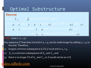
c[springtime, printing]
c[springtim, printing] c[springtime, printin]
[springti, printing] [springtim, printin] [springtim, printin] [springtime, printi]
[springt, printing] [springti, printin] [springtim, printi] [springtime, print]
video.edhole.com
Comp 122, Spring 2004](https://image.slidesharecdn.com/freevideolecturesformca-141101081237-conversion-gate01/85/Free-video-lectures-for-mca-14-320.jpg)
![Recursive Solution
a b
0 if empty or empty,
ì
ïî
ïí
c c prefix prefix
= a b + a =
b
max( [ , ], [ , ]) if end( ) end( ).
[ , ] 1 if end( ) end( ),
¹
[ , ]
a b a b a b
a b
c prefix c prefix
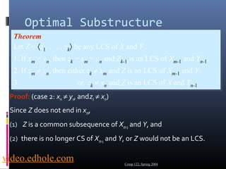
p r i n t i n g
s
p
r
i
n
g
t
i
m
e
Comp 122, Spring 2004
•Keep track of c[a,b] in a
table of nm entries:
•top/down
•bottom/up
video.edhole.com](https://image.slidesharecdn.com/freevideolecturesformca-141101081237-conversion-gate01/85/Free-video-lectures-for-mca-15-320.jpg)
![Computing the length of an LCS
LCS-LCS-LENGTH LENGTH ((X, X, Y)
Y)
1. 1. m m ← ← length[length[X]
X]
2. 2. n n ← ← length[length[Y]
Y]
3. 3. for for i i ← ← 1 1 to to m
m
4. 4. do do c[c[i, i, 0] 0] ← ← 0
0
5. 5. for for j j ← ← 0 0 to to n
n
6. 6. do do c[c[0, 0, j j ] ] ← ← 0
0
7. 7. for for i i ← ← 1 1 to to m
m
8. 8. do do for for j j ← ← 1 1 to to n
n
9. 9. do do if if xx= = yi yi j
j
10. 10. then then c[c[i, i, j j ] ] ← ← c[c[i-i-1, 1, j-j-1] 1] + + 1
1
11. 11. b[b[i, i, j j ] ] ← ← “ “ ”
”
12. 12. else else if if c[c[i-i-1, 1, j j ] ] ≥ ≥ c[c[i, i, j-j-1]
1]
13. 13. then then c[c[i, i, j j ] ] ← ← c[c[i- i- 1, 1, j j ]
]
14. 14. b[b[i, i, j j ] ] ← ← “↑”
“↑”
15. 15. else else c[c[i, i, j j ] ] ← ← c[c[i, i, j-j-1]
1]
16. 16. b[b[i, i, j j ] ] ← ← “←”
“←”
17. 17. return return c c and and b
b
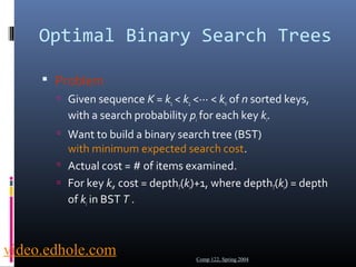
b[i, j ] points to table entry
whose subproblem we used
in solving LCS of Xi
and Yj.
c[m,n] contains the length
of an LCS of X and Y.
Time: O(mn)
Comp 122, Spring 2004
video.edhole.com](https://image.slidesharecdn.com/freevideolecturesformca-141101081237-conversion-gate01/85/Free-video-lectures-for-mca-16-320.jpg)
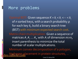
![Constructing an LCS
PRINT-LCS (b, X, i, j)
1. if i = 0 or j = 0
2. then return
3. if b[i, j ] = “ ”
4. then PRINT-LCS(b, X, i-1, j-1)
5. print xi
6. elseif b[i, j ] = “↑”
7. then PRINT-LCS(b, X, i-1, j)
8. else PRINT-LCS(b, X, i, j-1)
PRINT-LCS (b, X, i, j)
1. if i = 0 or j = 0
2. then return
3. if b[i, j ] = “ ”
4. then PRINT-LCS(b, X, i-1, j-1)
5. print xi
6. elseif b[i, j ] = “↑”
7. then PRINT-LCS(b, X, i-1, j)
8. else PRINT-LCS(b, X, i, j-1)
•Initial call is PRINT-LCS (b, X,m, n).
•When b[i, j ] = , we have extended LCS by one character. So
LCS = entries with in them.
•Time: O(m+n)
video.edhole.com
Comp 122, Spring 2004](https://image.slidesharecdn.com/freevideolecturesformca-141101081237-conversion-gate01/85/Free-video-lectures-for-mca-17-320.jpg)

![Expected Search Cost
[search cost in ]
å
k p
= + ×
(depth ( ) 1)
å å
k p p
= × +
depth ( )
T i i i
= =
1 1
n
å
=
=
= + ×
i
T i i
n
i
n
i
n
i
T i i
k p
E T
1
1
1 depth ( )
Sum of probabilities is 1.
(15.16)
Comp 122, Spring 2004
video.edhole.com](https://image.slidesharecdn.com/freevideolecturesformca-141101081237-conversion-gate01/85/Free-video-lectures-for-mca-20-320.jpg)
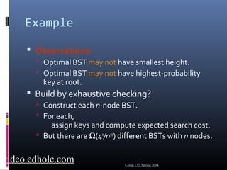
![Example
Consider 5 keys with these search probabilities:
p1 = 0.25, p2 = 0.2, p3 = 0.05, p4 = 0.2, p5 = 0.3.
Comp 122, Spring 2004
k2
k1 k4
k3 k5
i depthT(ki) depthT(ki)·pi
1 1 0.25
2 0 0
3 2 0.1
4 1 0.2
5 2 0.6
1.15
Therefore, E[search cost] = 2.15.
video.edhole.com](https://image.slidesharecdn.com/freevideolecturesformca-141101081237-conversion-gate01/85/Free-video-lectures-for-mca-21-320.jpg)
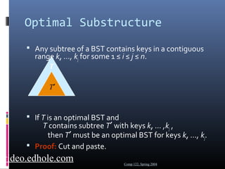
![Example
p1 = 0.25, p2 = 0.2, p3 = 0.05, p4 = 0.2, p5 = 0.3.
i depthT(ki) depthT(ki)·pi
1 1 0.25
2 0 0
3 3 0.15
4 2 0.4
5 1 0.3
1.10
Therefore, E[search cost] = 2.10.
Comp 122, Spring 2004
k2
k1 k5
k4
k3 This tree turns out to be optimal for this set of keys.
video.edhole.com](https://image.slidesharecdn.com/freevideolecturesformca-141101081237-conversion-gate01/85/Free-video-lectures-for-mca-22-320.jpg)
![Recursive Solution
Find optimal BST for ki,...,kj, where i ≥ 1, j ≤ n, j ≥ i-1.
When j = i-1, the tree is empty.
Define e[i, j ] = expected search cost of optimal BST for
ki,...,kj.
If j = i-1, then e[i, j ] = 0.
If j ≥ i,
Select a root kr, for some i ≤ r ≤ j .
Recursively make an optimal BSTs
for ki,..,kr-1 as the left subtree, and
for kr+1,..,kj as the right subtree.
Comp 122, Spring 2004 video.edhole.com](https://image.slidesharecdn.com/freevideolecturesformca-141101081237-conversion-gate01/85/Free-video-lectures-for-mca-26-320.jpg)
![Recursive Solution
When the OPT subtree becomes a subtree of a node:
Depth of every node in OPT subtree goes up by 1.
Expected search cost increases by
j
å=
w(i, j) =
p
l l i
from (15.16)
If kr is the root of an optimal BST for ki,..,kj :
e[i, j ] = pr + (e[i, r-1] + w(i, r-1))+(e[r+1, j] + w(r+1, j))
= e[i, r-1] + e[r+1, j] + w(i, j).
But, we don’t know kr. Hence,
0 if 1
ïî
ïí ì
j i
= -
- + + + £
=
min{ [ , 1] [ 1, ] ( , )} if
£ £
e i r e r j w i j i j
e i j
i r j
[ , ]
Comp 122, Spring 2004
(because w(i, j)=w(i,r-1) + pr + w(r + 1, j))
video.edhole.com](https://image.slidesharecdn.com/freevideolecturesformca-141101081237-conversion-gate01/85/Free-video-lectures-for-mca-27-320.jpg)
![Computing an Optimal
Solution
For each subproblem (i,j), store:
expected search cost in a table e[1 ..n+1 , 0 ..n]
Will use only entries e[i, j ], where j ≥ i-1.
root[i, j ] = root of subtree with keys ki,..,kj, for 1 ≤ i
≤ j ≤ n.
w[1..n+1, 0..n] = sum of probabilities
w[i, i-1] = 0 for 1 ≤ i ≤ n.
w[i, j ] = w[i, j-1] + pj for 1 ≤ i ≤ j ≤ n.
Comp 122, Spring 2004 video.edhole.com](https://image.slidesharecdn.com/freevideolecturesformca-141101081237-conversion-gate01/85/Free-video-lectures-for-mca-28-320.jpg)
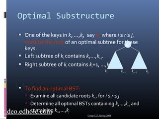
![Pseudo-code
OPTIMAL-BST(p, q, n)
1. for i ← 1 to n + 1
2. do e[i, i- 1] ← 0
3. w[i, i- 1] ← 0
4. for l ← 1 to n
5. do for i ← 1 to n-l + 1
6. do j ←i + l-1
7. e[i, j ]←∞
8. w[i, j ] ← w[i, j-1] + pj
9. for r ←i to j
10. do t ← e[i, r-1] + e[r + 1, j ] + w[i, j ]
11. if t < e[i, j ]
12. then e[i, j ] ← t
13. root[i, j ] ←r
14. return e and root
Comp 122, Spring 2004
Time: O(n3)
Consider all trees with l keys.
Fix the first key.
Fix the last key
Determine the root
of the optimal
(sub)tree
video.edhole.com](https://image.slidesharecdn.com/freevideolecturesformca-141101081237-conversion-gate01/85/Free-video-lectures-for-mca-29-320.jpg)


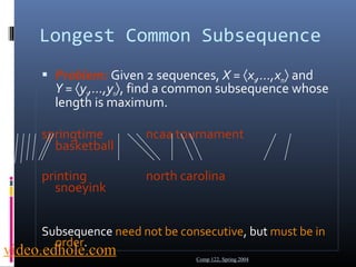
This document discusses the longest common subsequence problem and provides an example of how it can be solved using dynamic programming. It begins by defining the problem of finding the longest subsequence that is common to two input sequences. It then shows that this problem exhibits optimal substructure and can be solved recursively. However, a recursive solution is inefficient due to redundant subproblem computations. Instead, it presents an algorithm that uses dynamic programming to compute the length of the longest common subsequence in O(mn) time by filling out a 2D table in a bottom-up manner and returning the value at the last index. It also describes how to construct the actual longest common subsequence by tracing back through the table.