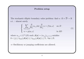
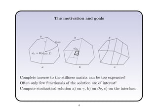
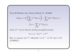
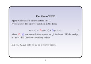
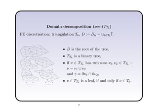
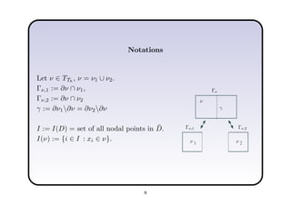
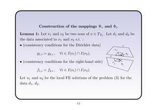
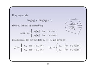
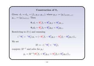
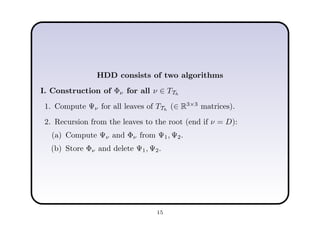
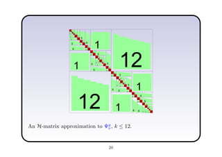
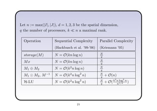
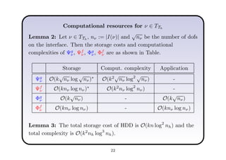
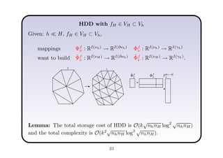
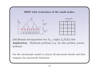
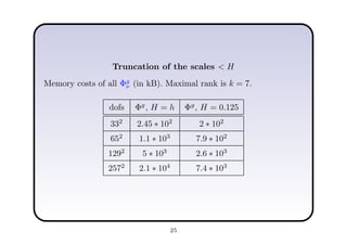
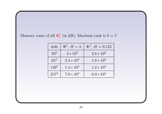
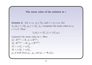
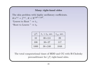
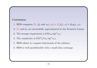
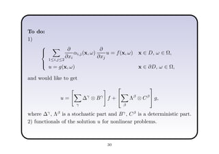
Application of H-matrices for solving
multiscale problems with stochastical right hand side
Litvinenko Alexander
WIRE, TU Braunschweig,
5 April, 2007.
www.hlib.org www.wire.tu-bs.de
1
Contents
1. Problem Setup
2. Hierarchical Domain Decomposition (HDD)
3. HDD in the H-matrix arithmetic
4. Computational resources of HDD
5. Functionals of the solution
6. Numerical results
2
Problem setup
The stochastic elliptic boundary value problem: find u : Ω × D → R
s.t. : almost surely



1≤i,j≤2
∂
∂xi
αi,j(x)
∂
∂xj
u = f(x, ω) on D
u = g(x, ω) in ∂D
(1)
where αi,j ∈ L∞
(D) such A(x) = (αi,j)i,j=1,2 satisfies
0 < λ ≤ λmin(A(x)) ≤ λmax(A(x)) ≤ λ , ∀x ∈ D.
⇒ Oscillatory or jumping coefficients are allowed.
3
The motivation and goals
a) b) c)
D
D D
u|∂Dγ
ν
u|∂ν
u|γ = Φ(u|∂D, f)
Complete inverse to the stiffness matrix can be too expensive!
Often only few functionals of the solution are of interest!
Compute stochastical solution a) on γ, b) on ∂ν, c) on the interface.
4
From H.Matthies and A.Keese Bericht Nr. 08-2003
K˜u(ω) = K
α∈J
u(α)
Hα(ω) =
α∈J
Ku(α)
Hα(ω) =
˜f(ω) =
α∈J
f(α)
Hα(ω).
where u(α)
can by find by solving uncoupled systems
∀α ∈ J : Ku(α)
= f(α)
.
How to compute all u(α)
efficiently? a) K−1
, b) LU and c) CG
(GMRES)?
5
The idea of HDD
Apply Galerkin FE discretisation to (1).
We construct the discrete solution in the form
uh(·, ω) = Fhfh(·, ω) + Ghgh(·, ω), (2)
where Fh, Gh are two solution operators, fh is the st. FE rhs and gh
is the st. FE Dirichlet-boundary values.
E.g. uh(fh, gh) only for fh in a coarser space.
6
Domain decomposition tree (TTh
)
FE discretisation: triangulation Th, D := Dh = ∪t∈Th
t.
1
2
3
4
5
6
7
9
10
11
12
13
14
15
8
5
6
7
11
12
13
14
15
8
1
2
3
4
5
6
7
9
10
3
4
1
9
10
......
5
6
11
12
13
14
15
6
7
11
15
8
......
2
6
2
6
• D is the root of the tree,
• TTh
is a binary tree,
• if ν ∈ TTh
has two sons ν1, ν2 ∈ TTh
:
ν = ν1 ∪ ν2
and γ = ∂ν1 ∩ ∂ν2,
• ν ∈ TTh
is a leaf, if and only if ν ∈ Th.
7
Notations
Let ν ∈ TTh
, ν = ν1 ∪ ν2.
Γν,1 := ∂ν ∩ ν1,
Γν,2 := ∂ν ∩ ν2
γ := ∂ν1∂ν = ∂ν2∂ν
I := I(D) = set of all nodal points in ¯D.
I(ν) := {i ∈ I : xi ∈ ν}.
1 2
γ
Γν,1 Γν,2
Γν
ν
νν
8
FE Galerkin Discretisation
For ν ∈ TTh
define fν := (fi)i∈I(ν), gν := (gi)i∈I(∂ν), dν := (fν, gν).
Let bj, j = 1, ..., N be a piecewise linear basis,
Vh := span{b1, ..., bN }, Vh ⊂ V = H1
(D).
Variational Galerkin formulation of (1): find uh ∈ Vh such that



aν(uh, bj) = (fν, bj)L2(ν) ∀ j ∈ I(
◦
ν),
uh(xj) = gj ∀ j ∈ I(∂ν),
(3)
where
aν(bi, bj) =
D
α(x)(∇bi, ∇bj)dx,
(fν, bj) =
suppbj
fνbjdx.
9
Let Uν ∈ Vh be the solution of (3), then Uν = Uf
ν + Ug
ν ,
where Uf
ν is the solution of



aν(Uf
ν , bj) = (fν, bj)L2(ν) , ∀ j ∈ I(
◦
ν),
Uf
ν (xj) = 0, ∀ j ∈ I(∂ν)
and Ug
ν is the solution of



aν(Ug
ν , bj) = 0, ∀ j ∈ I(
◦
ν),
Ug
ν (xj) = gj, ∀ j ∈ I(∂ν).
10
Main point of HDD is to build the mapping Φν := (Φg
ν, Φf
ν ), where
Φg
ν : RI(∂ν)
→ RI(γ)
and Φf
ν : RI(ν)
→ RI(γ)
for each ν ∈ TTh
.
1. Definition of Mapping Φν
(Φν(dν))i := uh(xi) , ∀i ∈ I(γ).
Hence, Φν(dν) is the trace of uh on γ.
Actually, Φνdν = Φg
νgν + Φf
ν fν.
2. Definition of auxiliary Mapping Ψν := (Ψg
ν, Ψf
ν )
Ψν(d) = (Ψν(dν))i∈I(∂ν) with (Ψν(dν))i := aν(uh, bi) − (fν, bi)L2(ν) ,
Ψνdν = Ψf
ν fν + Ψg
νgν.
11
Construction of the mappings Ψν and Φν
Lemma 1: Let ν1 and ν2 be two sons of ν ∈ TTh
. Let d1 and d2 be
the data associated to ν1 and ν2 s.t. :
• (consistency conditions for the Dirichlet data)
g1,i = g2,i , ∀i ∈ I(ν1) ∩ I(ν2),
• (consistency conditions for the right-hand side)
f1,i = f2,i , ∀i ∈ I(ν1) ∩ I(ν2).
1
2
xj
γ
xj
ν
ν
ν
Let u1 and u2 be the local FE solutions of the problem (3) for the
data d1, d2.
12
If u1, u2 satisfy
γ
Ψ1(d1) + γ
Ψ2(d2) = 0,
then uν defined by assembling
uν(xi) :=



u1(xi) for i ∈ I(ν1)
u2(xi) for i ∈ I(ν2)
1
2
xj
γ
xj
ν
ν
ν
is solution of (3) for the data dν = (fν, gν) given by
fν :=



f1,i for i ∈ I(ν1)
f2,i for i ∈ I(ν2)
gν :=



g1,i for i ∈ I(∂ν1)
g2,i for i ∈ I(∂ν2)
13
Construction of Φν
Given: d1 := dν1 = (f1, g1,Γ, g1,γ), where g1,Γ := (g1)i∈I(Γν,1),
g1,γ := (g1)i∈I(γ). Then
Ψ1d1 = Ψf
1 f1 + ΨΓ
1 g1,Γ + Ψγ
1 g1,γ,
Ψ2d2 = Ψf
2 f2 + ΨΓ
2 g2,Γ + Ψγ
2 g2,γ.
Restricting to I(γ) and summing
( γ
Ψγ
1 + γ
Ψγ
2 ) gγ = (−Ψf
1 f1 − ΨΓ
1 g1,Γ − Ψf
2 f2 − ΨΓ
2 g2,Γ)|γ.
We set
M := −( γ
Ψγ
1 + γ
Ψγ
2 ),
compute M−1
and solve for gγ:
gγ = M−1
(Ψf
1 f1 + ΨΓ
1 g1,Γ + Ψf
2 f2 + ΨΓ
2 g2,Γ)|γ.
14
HDD consists of two algorithms
I. Construction of Φν for all ν ∈ TTh
1. Compute Ψν for all leaves of TTh
(∈ R3×3
matrices).
2. Recursion from the leaves to the root (end if ν = D):
(a) Compute Ψν and Φν from Ψ1, Ψ2.
(b) Store Φν and delete Ψ1, Ψ2.
15
II. Application of Φν
1. Given dν = (fν, gν), compute the solution uh on the interface γ
by Φν(dν).
2. Build the data d1 = (fν1 , gν1 ), d2 = (fν2 , gν2 ) from dν = (fν, gν)
and gγ = Φν(dν).
3. Repeat for sons of ν1 and ν2.
16
HDD in the H-matrix arithmetic
The system of linear equations for ν ∈ TTh
is Au = Fc.
Rewrite it in the block matrix form:


ABB ABI
AIB AII




uB
uI

 =


FB
FI

 c,
where uB ∈ RI(∂ν)
, uI ∈ RI(γ)
, c ∈ RI(ν)
ABB ∈ RI(∂ν)
→ RI(∂ν)
, AII ∈ RI(γ)
→ RI(γ)
.
17
Eliminate uI:


ABB − ABIA−1
II AIB 0
AIB AII




uB
uI

 =


FB − ABIA−1
II FI
FI

 c.
(ABB − ABIA−1
II AIB)uB = (FB − ABIA−1
II FI)c
uI = A−1
II FIc − A−1
II AIBuB,
Ψg
ν :=ABB − ABIA−1
II AIB (Schur complement)
Ψf
ν :=FB − ABIA−1
II FI,
Φg
ν :=A−1
II AIB
Φf
ν :=A−1
II FI.
Exact HDD requires expensive matrix arithmetic.
Apply the H-matrix techniques.
18
H-matrices (Hackbusch ’99)
Rank-k matrices
R ∈ Rn×m
, A ∈ Rn×k
, B ∈ Rm×k
, k ≪ min(n, m).
The storage R = ABT
is k(n + m) instead of n · m for R represented
in the full matrix format.
=
A
B
T
*
R
k
k
n
m
n
m
19
25 4
4 8
5
5 16 5
5 16
5
5 32 6
6 32
5
5
32 5
5 32
6
6
32 5
5 32
1
1
32 5
5 32 5
5
32 5
5
16 4
4 32 5
5 16
5
5 32
5
5
32 5
5 32
12
12
32 5
5 32 5
5
32 5
5
16 5
5
32 4
4 16
5
5 32
5
5
32 5
5 32
1
1
32 5
5 32 6
6
32 5
5 32 6
6
32 5
5
32 5
5
16 5
5
16 4
4 31
An H-matrix approximation to Ψg
ν, k ≤ 12.
20
Let n := max(|I|, |J|), d = 1, 2, 3 be the spatial dimension,
q the number of processors, k ≪ n a maximal rank.
Operation Sequential Complexity Parallel Complexity
(Hackbusch et al. ’99-’06) (Kriemann ’05)
storage(M) N = O(kn log n) N
q
Mx N = O(kn log n) N
q
M1 ⊕ M2 N = O(k2
n log n) N
q
M1 ⊙ M2, M−1
N = O(k2
n log2
n) N
q + O(n)
H-LU N = O(k2
n log2
n) N
q + O(k2
n log2
n
n1/d )
21
Computational resources for ν ∈ TTh
Lemma 2: Let ν ∈ TTh
, nν := |I(ν)| and
√
nν be the number of dofs
on the interface. Then the storage costs and computational
complexities of Ψg
ν, Ψf
ν , Φg
ν, Φf
ν are as shown in Table.
Storage Comput. complexity Application
Ψg
ν O(k
√
nν log
√
nν)∗
O(k2√
nν log2 √
nν) -
Ψf
ν O(knν log nν)∗
O(k2
nν log2
nν) -
Φg
ν O(k
√
nν) - O(k
√
nν)
Φf
ν O(knν log nν) - O(knν log nν)
Lemma 3: The total storage cost of HDD is O(kn log2
nh) and the
total complexity is O(k2
nh log3
nh).
22
HDD with fH ∈ VH ⊂ Vh
Given: h ≪ H, fH ∈ VH ⊂ Vh,
mappings Ψf
ν : RI(νh)
→ RI(∂νh)
Φf
ν : RI(νh)
→ RI(γh)
want to build ˜Ψf
ν : RI(νH )
→ RI(∂νh) ˜Φf
ν : RI(νH )
→ RI(γh)
.
H h
.
=
Φf
ν
˜Φf
ν Ph←H
ν
Lemma: The total storage cost of HDD is O(k
√
nhnH log2 √
nhnH)
and the total complexity is O(k2√
nhnH log3 √
nhnH ).
23
HDD with truncation of the small scales:
D
h
H
T≥H
Th
TTh
T<H
Th
. . . .
.
.
.
.
.
.
.
.
.
.
.
.
mean value
(left)Domain decomposition tree TTh
; (right) 2
√
nhnH dofs.
Application: Multiscale problems (e.g. the skin problem, porous
medium).
Use the microscopic model to extract all microscale details and then
compute the macroscale behaviour.
24
Truncation of the scales < H
Memory costs of all Φg
ν (in kB). Maximal rank is k = 7.
dofs Φg
, H = h Φg
, H = 0.125
332
2.45 ∗ 102
2 ∗ 102
652
1.1 ∗ 103
7.9 ∗ 102
1292
5 ∗ 103
2.6 ∗ 103
2572
2.1 ∗ 104
7.4 ∗ 103
25
Memory costs of all Φf
ν (in kB). Maximal rank is k = 7.
dofs Φf
, H = h Φf
, H = 0.125
332
4 ∗ 102
2.8 ∗ 102
652
2.4 ∗ 103
1.8 ∗ 103
1292
1.4 ∗ 104
1.2 ∗ 104
2572
7.9 ∗ 104
6.9 ∗ 104
26
The mean value of the solution in ν
Lemma 4: Let ν, ν1, ν2 ∈ TTh
and ν = ν1 ∪ ν2. Let
λνi (dνi ) = (λg
νi
, gνi ) + (λf
νi
, fνi ) computes the mean value in νi,
i = 1, 2. Then
λν(dν) = (λf
ν , fν) + (λg
ν, gν)
computes the mean value in ν. Here
λf
ν : RI(ν)
→ R, fν ∈ RI(ν)
,
λg
ν : RI(∂ν)
→ R, gν ∈ RI(∂ν)
,
λf
ν = c1λf
ν1
+ c2λf
ν2
,
λg
ν = c1λg
ν1
+ c2λg
ν2
,
gν is built from gν1 , gν2 and g|γ := Φν(dν).
27
Many right-hand sides
The skin problem with highly oscillatory coefficients.
Ku(α)
= f(α)
, K ∈ R1292
×1292
.
“Leaves to Root ” ⇒ t1,
“Root to Leaves ” ⇒ t2.
|J | t1 + t2, sec. tcg, sec.
10 38+2.8 29
100 38+27 117
1000 38+240 1048
The total computational times of HDD and CG with H-Cholesky
preconditioner for |J | right-hand sides.
28
Conclusion:
1. HDD computes Fh, Gh and uh(·, ω) = Fhfh(·, ω) + Ghgh(·, ω).
2. Fh and Gh are successfully approximated in the H-matrix format.
3. The storage requirement is O(knh log2
nh).
4. The complexity is O(k2
|J |nh log3
nh).
5. HDD allows to compute functionals of the solution.
6. HDD is well parallelizable with a small data exchange.
29
To do:
1)



1≤i,j≤2
∂
∂xi
αi,j(x, ω)
∂
∂xj
u = f(x, ω) x ∈ D, ω ∈ Ω,
u = g(x, ω) x ∈ ∂D, ω ∈ Ω,
and would like to get
u =
γ
∆γ
⊗ Bγ
f +


β
Λβ
⊗ Cβ

 g,
where ∆γ
, Λβ
is a stochastic part and Bγ
, Cβ
is a deterministic part.
2) functionals of the solution u for nonlinear problems.
30
Thanks for your attention!
Questions ?
31
32

My PhD talk "Application of H-matrices for computing partial inverse"

  • 1.
    Application of H-matricesfor solving multiscale problems with stochastical right hand side Litvinenko Alexander WIRE, TU Braunschweig, 5 April, 2007. www.hlib.org www.wire.tu-bs.de 1
  • 2.
    Contents 1. Problem Setup 2.Hierarchical Domain Decomposition (HDD) 3. HDD in the H-matrix arithmetic 4. Computational resources of HDD 5. Functionals of the solution 6. Numerical results 2
  • 3.
    Problem setup The stochasticelliptic boundary value problem: find u : Ω × D → R s.t. : almost surely    1≤i,j≤2 ∂ ∂xi αi,j(x) ∂ ∂xj u = f(x, ω) on D u = g(x, ω) in ∂D (1) where αi,j ∈ L∞ (D) such A(x) = (αi,j)i,j=1,2 satisfies 0 < λ ≤ λmin(A(x)) ≤ λmax(A(x)) ≤ λ , ∀x ∈ D. ⇒ Oscillatory or jumping coefficients are allowed. 3
  • 4.
    The motivation andgoals a) b) c) D D D u|∂Dγ ν u|∂ν u|γ = Φ(u|∂D, f) Complete inverse to the stiffness matrix can be too expensive! Often only few functionals of the solution are of interest! Compute stochastical solution a) on γ, b) on ∂ν, c) on the interface. 4
  • 5.
    From H.Matthies andA.Keese Bericht Nr. 08-2003 K˜u(ω) = K α∈J u(α) Hα(ω) = α∈J Ku(α) Hα(ω) = ˜f(ω) = α∈J f(α) Hα(ω). where u(α) can by find by solving uncoupled systems ∀α ∈ J : Ku(α) = f(α) . How to compute all u(α) efficiently? a) K−1 , b) LU and c) CG (GMRES)? 5
  • 6.
    The idea ofHDD Apply Galerkin FE discretisation to (1). We construct the discrete solution in the form uh(·, ω) = Fhfh(·, ω) + Ghgh(·, ω), (2) where Fh, Gh are two solution operators, fh is the st. FE rhs and gh is the st. FE Dirichlet-boundary values. E.g. uh(fh, gh) only for fh in a coarser space. 6
  • 7.
    Domain decomposition tree(TTh ) FE discretisation: triangulation Th, D := Dh = ∪t∈Th t. 1 2 3 4 5 6 7 9 10 11 12 13 14 15 8 5 6 7 11 12 13 14 15 8 1 2 3 4 5 6 7 9 10 3 4 1 9 10 ...... 5 6 11 12 13 14 15 6 7 11 15 8 ...... 2 6 2 6 • D is the root of the tree, • TTh is a binary tree, • if ν ∈ TTh has two sons ν1, ν2 ∈ TTh : ν = ν1 ∪ ν2 and γ = ∂ν1 ∩ ∂ν2, • ν ∈ TTh is a leaf, if and only if ν ∈ Th. 7
  • 8.
    Notations Let ν ∈TTh , ν = ν1 ∪ ν2. Γν,1 := ∂ν ∩ ν1, Γν,2 := ∂ν ∩ ν2 γ := ∂ν1∂ν = ∂ν2∂ν I := I(D) = set of all nodal points in ¯D. I(ν) := {i ∈ I : xi ∈ ν}. 1 2 γ Γν,1 Γν,2 Γν ν νν 8
  • 9.
    FE Galerkin Discretisation Forν ∈ TTh define fν := (fi)i∈I(ν), gν := (gi)i∈I(∂ν), dν := (fν, gν). Let bj, j = 1, ..., N be a piecewise linear basis, Vh := span{b1, ..., bN }, Vh ⊂ V = H1 (D). Variational Galerkin formulation of (1): find uh ∈ Vh such that    aν(uh, bj) = (fν, bj)L2(ν) ∀ j ∈ I( ◦ ν), uh(xj) = gj ∀ j ∈ I(∂ν), (3) where aν(bi, bj) = D α(x)(∇bi, ∇bj)dx, (fν, bj) = suppbj fνbjdx. 9
  • 10.
    Let Uν ∈Vh be the solution of (3), then Uν = Uf ν + Ug ν , where Uf ν is the solution of    aν(Uf ν , bj) = (fν, bj)L2(ν) , ∀ j ∈ I( ◦ ν), Uf ν (xj) = 0, ∀ j ∈ I(∂ν) and Ug ν is the solution of    aν(Ug ν , bj) = 0, ∀ j ∈ I( ◦ ν), Ug ν (xj) = gj, ∀ j ∈ I(∂ν). 10
  • 11.
    Main point ofHDD is to build the mapping Φν := (Φg ν, Φf ν ), where Φg ν : RI(∂ν) → RI(γ) and Φf ν : RI(ν) → RI(γ) for each ν ∈ TTh . 1. Definition of Mapping Φν (Φν(dν))i := uh(xi) , ∀i ∈ I(γ). Hence, Φν(dν) is the trace of uh on γ. Actually, Φνdν = Φg νgν + Φf ν fν. 2. Definition of auxiliary Mapping Ψν := (Ψg ν, Ψf ν ) Ψν(d) = (Ψν(dν))i∈I(∂ν) with (Ψν(dν))i := aν(uh, bi) − (fν, bi)L2(ν) , Ψνdν = Ψf ν fν + Ψg νgν. 11
  • 12.
    Construction of themappings Ψν and Φν Lemma 1: Let ν1 and ν2 be two sons of ν ∈ TTh . Let d1 and d2 be the data associated to ν1 and ν2 s.t. : • (consistency conditions for the Dirichlet data) g1,i = g2,i , ∀i ∈ I(ν1) ∩ I(ν2), • (consistency conditions for the right-hand side) f1,i = f2,i , ∀i ∈ I(ν1) ∩ I(ν2). 1 2 xj γ xj ν ν ν Let u1 and u2 be the local FE solutions of the problem (3) for the data d1, d2. 12
  • 13.
    If u1, u2satisfy γ Ψ1(d1) + γ Ψ2(d2) = 0, then uν defined by assembling uν(xi) :=    u1(xi) for i ∈ I(ν1) u2(xi) for i ∈ I(ν2) 1 2 xj γ xj ν ν ν is solution of (3) for the data dν = (fν, gν) given by fν :=    f1,i for i ∈ I(ν1) f2,i for i ∈ I(ν2) gν :=    g1,i for i ∈ I(∂ν1) g2,i for i ∈ I(∂ν2) 13
  • 14.
    Construction of Φν Given:d1 := dν1 = (f1, g1,Γ, g1,γ), where g1,Γ := (g1)i∈I(Γν,1), g1,γ := (g1)i∈I(γ). Then Ψ1d1 = Ψf 1 f1 + ΨΓ 1 g1,Γ + Ψγ 1 g1,γ, Ψ2d2 = Ψf 2 f2 + ΨΓ 2 g2,Γ + Ψγ 2 g2,γ. Restricting to I(γ) and summing ( γ Ψγ 1 + γ Ψγ 2 ) gγ = (−Ψf 1 f1 − ΨΓ 1 g1,Γ − Ψf 2 f2 − ΨΓ 2 g2,Γ)|γ. We set M := −( γ Ψγ 1 + γ Ψγ 2 ), compute M−1 and solve for gγ: gγ = M−1 (Ψf 1 f1 + ΨΓ 1 g1,Γ + Ψf 2 f2 + ΨΓ 2 g2,Γ)|γ. 14
  • 15.
    HDD consists oftwo algorithms I. Construction of Φν for all ν ∈ TTh 1. Compute Ψν for all leaves of TTh (∈ R3×3 matrices). 2. Recursion from the leaves to the root (end if ν = D): (a) Compute Ψν and Φν from Ψ1, Ψ2. (b) Store Φν and delete Ψ1, Ψ2. 15
  • 16.
    II. Application ofΦν 1. Given dν = (fν, gν), compute the solution uh on the interface γ by Φν(dν). 2. Build the data d1 = (fν1 , gν1 ), d2 = (fν2 , gν2 ) from dν = (fν, gν) and gγ = Φν(dν). 3. Repeat for sons of ν1 and ν2. 16
  • 17.
    HDD in theH-matrix arithmetic The system of linear equations for ν ∈ TTh is Au = Fc. Rewrite it in the block matrix form:   ABB ABI AIB AII     uB uI   =   FB FI   c, where uB ∈ RI(∂ν) , uI ∈ RI(γ) , c ∈ RI(ν) ABB ∈ RI(∂ν) → RI(∂ν) , AII ∈ RI(γ) → RI(γ) . 17
  • 18.
    Eliminate uI:   ABB −ABIA−1 II AIB 0 AIB AII     uB uI   =   FB − ABIA−1 II FI FI   c. (ABB − ABIA−1 II AIB)uB = (FB − ABIA−1 II FI)c uI = A−1 II FIc − A−1 II AIBuB, Ψg ν :=ABB − ABIA−1 II AIB (Schur complement) Ψf ν :=FB − ABIA−1 II FI, Φg ν :=A−1 II AIB Φf ν :=A−1 II FI. Exact HDD requires expensive matrix arithmetic. Apply the H-matrix techniques. 18
  • 19.
    H-matrices (Hackbusch ’99) Rank-kmatrices R ∈ Rn×m , A ∈ Rn×k , B ∈ Rm×k , k ≪ min(n, m). The storage R = ABT is k(n + m) instead of n · m for R represented in the full matrix format. = A B T * R k k n m n m 19
  • 20.
    25 4 4 8 5 516 5 5 16 5 5 32 6 6 32 5 5 32 5 5 32 6 6 32 5 5 32 1 1 32 5 5 32 5 5 32 5 5 16 4 4 32 5 5 16 5 5 32 5 5 32 5 5 32 12 12 32 5 5 32 5 5 32 5 5 16 5 5 32 4 4 16 5 5 32 5 5 32 5 5 32 1 1 32 5 5 32 6 6 32 5 5 32 6 6 32 5 5 32 5 5 16 5 5 16 4 4 31 An H-matrix approximation to Ψg ν, k ≤ 12. 20
  • 21.
    Let n :=max(|I|, |J|), d = 1, 2, 3 be the spatial dimension, q the number of processors, k ≪ n a maximal rank. Operation Sequential Complexity Parallel Complexity (Hackbusch et al. ’99-’06) (Kriemann ’05) storage(M) N = O(kn log n) N q Mx N = O(kn log n) N q M1 ⊕ M2 N = O(k2 n log n) N q M1 ⊙ M2, M−1 N = O(k2 n log2 n) N q + O(n) H-LU N = O(k2 n log2 n) N q + O(k2 n log2 n n1/d ) 21
  • 22.
    Computational resources forν ∈ TTh Lemma 2: Let ν ∈ TTh , nν := |I(ν)| and √ nν be the number of dofs on the interface. Then the storage costs and computational complexities of Ψg ν, Ψf ν , Φg ν, Φf ν are as shown in Table. Storage Comput. complexity Application Ψg ν O(k √ nν log √ nν)∗ O(k2√ nν log2 √ nν) - Ψf ν O(knν log nν)∗ O(k2 nν log2 nν) - Φg ν O(k √ nν) - O(k √ nν) Φf ν O(knν log nν) - O(knν log nν) Lemma 3: The total storage cost of HDD is O(kn log2 nh) and the total complexity is O(k2 nh log3 nh). 22
  • 23.
    HDD with fH∈ VH ⊂ Vh Given: h ≪ H, fH ∈ VH ⊂ Vh, mappings Ψf ν : RI(νh) → RI(∂νh) Φf ν : RI(νh) → RI(γh) want to build ˜Ψf ν : RI(νH ) → RI(∂νh) ˜Φf ν : RI(νH ) → RI(γh) . H h . = Φf ν ˜Φf ν Ph←H ν Lemma: The total storage cost of HDD is O(k √ nhnH log2 √ nhnH) and the total complexity is O(k2√ nhnH log3 √ nhnH ). 23
  • 24.
    HDD with truncationof the small scales: D h H T≥H Th TTh T<H Th . . . . . . . . . . . . . . . . mean value (left)Domain decomposition tree TTh ; (right) 2 √ nhnH dofs. Application: Multiscale problems (e.g. the skin problem, porous medium). Use the microscopic model to extract all microscale details and then compute the macroscale behaviour. 24
  • 25.
    Truncation of thescales < H Memory costs of all Φg ν (in kB). Maximal rank is k = 7. dofs Φg , H = h Φg , H = 0.125 332 2.45 ∗ 102 2 ∗ 102 652 1.1 ∗ 103 7.9 ∗ 102 1292 5 ∗ 103 2.6 ∗ 103 2572 2.1 ∗ 104 7.4 ∗ 103 25
  • 26.
    Memory costs ofall Φf ν (in kB). Maximal rank is k = 7. dofs Φf , H = h Φf , H = 0.125 332 4 ∗ 102 2.8 ∗ 102 652 2.4 ∗ 103 1.8 ∗ 103 1292 1.4 ∗ 104 1.2 ∗ 104 2572 7.9 ∗ 104 6.9 ∗ 104 26
  • 27.
    The mean valueof the solution in ν Lemma 4: Let ν, ν1, ν2 ∈ TTh and ν = ν1 ∪ ν2. Let λνi (dνi ) = (λg νi , gνi ) + (λf νi , fνi ) computes the mean value in νi, i = 1, 2. Then λν(dν) = (λf ν , fν) + (λg ν, gν) computes the mean value in ν. Here λf ν : RI(ν) → R, fν ∈ RI(ν) , λg ν : RI(∂ν) → R, gν ∈ RI(∂ν) , λf ν = c1λf ν1 + c2λf ν2 , λg ν = c1λg ν1 + c2λg ν2 , gν is built from gν1 , gν2 and g|γ := Φν(dν). 27
  • 28.
    Many right-hand sides Theskin problem with highly oscillatory coefficients. Ku(α) = f(α) , K ∈ R1292 ×1292 . “Leaves to Root ” ⇒ t1, “Root to Leaves ” ⇒ t2. |J | t1 + t2, sec. tcg, sec. 10 38+2.8 29 100 38+27 117 1000 38+240 1048 The total computational times of HDD and CG with H-Cholesky preconditioner for |J | right-hand sides. 28
  • 29.
    Conclusion: 1. HDD computesFh, Gh and uh(·, ω) = Fhfh(·, ω) + Ghgh(·, ω). 2. Fh and Gh are successfully approximated in the H-matrix format. 3. The storage requirement is O(knh log2 nh). 4. The complexity is O(k2 |J |nh log3 nh). 5. HDD allows to compute functionals of the solution. 6. HDD is well parallelizable with a small data exchange. 29
  • 30.
    To do: 1)    1≤i,j≤2 ∂ ∂xi αi,j(x, ω) ∂ ∂xj u= f(x, ω) x ∈ D, ω ∈ Ω, u = g(x, ω) x ∈ ∂D, ω ∈ Ω, and would like to get u = γ ∆γ ⊗ Bγ f +   β Λβ ⊗ Cβ   g, where ∆γ , Λβ is a stochastic part and Bγ , Cβ is a deterministic part. 2) functionals of the solution u for nonlinear problems. 30
  • 31.
    Thanks for yourattention! Questions ? 31
  • 32.