The document discusses Bode plots, which are used to analyze the frequency response of linear systems. Bode plots graphically represent the magnitude and phase of a system's frequency response. They are constructed by plotting the logarithm of frequency versus gain in decibels and phase in degrees. The document outlines how to construct Bode plots based on different factors in a system's transfer function, including constants, poles, zeros, and complex terms. It provides examples of Bode plots for various transfer functions and discusses how to determine a system's transfer function based on its Bode plot characteristics.

1. BODE PLOT
Dr.R.Subasri
Professor, Kongu Engineering College,
Perundurai, Erode, Tamilnadu, INDIA
1Dr.R.Subasri,KEC,INDIA

2. 2
Frequency Response Techniques
• Analysing the system on frequency basis
e.g communication systems
• Developed by Nyquist and Bode in 1930
• Older than root locus method given by
Evan in 1948
Dr.R.Subasri,KEC,INDIA

3. 3
Frequency Response Techniques
– Radio telescopes used for deep space
communication require precise positioning to
function effectively. To achieve a high degree
of precision ,an accurate mathematical model
of antenna dynamics is to used.
– To construct the model, engineers can test
the antenna by vibrating it with sinusoidal
forces of different frequencies and measuring
the vibrations. These measurements form the
basis for the model.
Dr.R.Subasri,KEC,INDIA

4. 4
Chapter objectives
• Definition of frequency response
• How to plot frequency response
• How to use frequency response to analyse
stability
• How to use frequency response to design
the gain to meet stability specifications.
Dr.R.Subasri,KEC,INDIA

5. 5
Frequency Response Techniques
-Advantages
• modelling transfer functions from physical
data.
• Designing compensators to meet steady
state error and transient response
requirements.
• Finding stability of systems
Dr.R.Subasri,KEC,INDIA

6. 6
Frequency Response
• In the steady state,
sinusoidal inputs to a
linear system
generate sinusoidal
responses of the
same frequency.
• But output differs in
amplitudes and phase
angle from the input
• Differences are
function of frequency.
Dr.R.Subasri,KEC,INDIA

7. 7
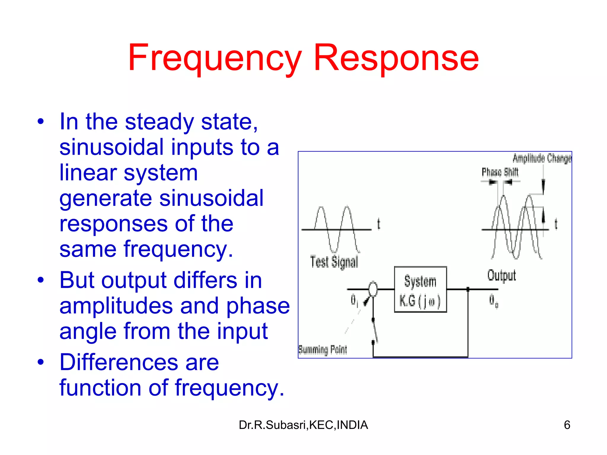
Frequency Response
)(
)(
)(



i
o
M
M
M =
)()()(  io −=
)()(  M
)()(  iiM  )()(  ooM 
)()(  ooM  = )]()([)()(  + iMiM
Magnitude frequency response =
Phase frequency response =
Combination of magnitude and phase frequency responses is Frequency
response
In general Frequency response of a system with transfer function G(s) is
)()(  M
 jSsGjG →= /)()(Dr.R.Subasri,KEC,INDIA

8. 8
Frequency response plots
❖Bode plot(or)Asymptotic
Approximation Plot (or)Logarithmic
plot
❖Polar plot – Nyquist plot
❖Log Magnitude Vs phase angle
Dr.R.Subasri,KEC,INDIA

9. 9
Logarithmic Frequency Scales
On a logarithmic scale, the variable is multiplied by a
given factor for equal increments of length along the
axis.
Decade Change –log10
Octave change – log2
Dr.R.Subasri,KEC,INDIA

10. 10
Bode Plot
• Factors of a transfer function
• Constant term K
• - Pure Differentiator-zero at origin -s
-Pure Integrator – pole at origin-1/s
• First order terms
- zero at real axis 1+s
-pole at real axis 1/1+s
• Second order terms
- complex zero s2+2ns+ n
2
-complex pole 1/ s2+2ns+n
2
Dr.R.Subasri,KEC,INDIA

11. 11
Constant K
consatnt factor G(s) = K
-20
0
20
40
0.1 1 10 100
log w
magnitudeindb
consatnt factor G(s) = K
-90
-45
0
45
90
0.1 1 10 100
log w
phaseangleindeg
Magnitude plot is constant and independent of frequency
Phase plot is constant at zero and independent of
frequency
Dr.R.Subasri,KEC,INDIA

12. 12
Pure Integrator 1/s
pure integrator-pole at origin G(s)=1/s
-40
-20
0
20
40
0.1 1 10 100
logw
magindb
Pure Integrator G(s) = 1 / s
-180
-135
-90
-45
0
45
90
0.1 1 10 100
log w
phaseangleindeg
starting point of magnitude plot is - 20 log  , where  is
the starting frequency in the plot. The plot starts from that
point and has the slope of - 20 db / dec.
Phase angle is - 90 - a straight line with no slope
Dr.R.Subasri,KEC,INDIA

13. 13
Pure Differentiator- s
pure differentiator-zero at origin G(s)=s
-40
-20
0
20
40
0.1 1 10 100
logw
magindb
Pure Differentiator G(s) = s
-90
-45
0
45
90
135
180
0.1 1 10 100
log w
phaseangleindeg
starting point of magnitude plot is + 20 log  , where  is
the starting frequency in the plot. The plot starts from
that point and has the slope of + 20 db / dec.
Phase angle is + 90 - a straight line with no slopeDr.R.Subasri,KEC,INDIA

14. 14
Zero at real axis - 1+s
first order term-zero at real axis
G(s)=1+sT
-40
-20
0
20
40
0.1/T 1/T 10/T 100/T
logwT
magindb
First order term-zero at real axis G(s)=1+sT
-90
-45
0
45
90
135
180
0.1/T 1/T 10/T 100/T
log wT
phaseangleindeg
For a constant zero at real axis, in low frequency region, phase angle
is 0 and in high frequency region, phase angle is + 90,in between the
slope is + 45 / dec.
For a constant zero at real axis, find the corner frequency c = 1/T.Up
to c,the magnitude plot is a straight line at 0 db and beyond c, the
plot has a line of slope + 20 db / dec.Dr.R.Subasri,KEC,INDIA

15. 15
Pole at real axis - 1/s+T
For a constant pole at real axis, in low frequency region, phase angle is
0 and in high frequency region, phase angle is -90,in between the
slope is - 45 / dec.
For a constant zero at real axis, find the corner frequency c = T. Up to
c,the magnitude plot is a straight line at 0 db and beyond c, the plot
has a line of slope - 20 db / dec.
Dr.R.Subasri,KEC,INDIA

16. 16
Complex zero - s2+2ns+n
2
second order term- complex zero
-40
-20
0
20
40
60
80
100
0.1 1 10 100
log w
magindb
second order term- complex zero
-180
-135
-90
-45
0
45
90
135
180
0.1 1 10 100
log w
phaseangleindeg
For a complex zero, find the corner frequency c =n .Up to c,the
magnitude plot is a straight line at +40 log n and beyond c, the plot
has a line of slope + 40 db / dec.
For a complex zero, in low frequency region, phase angle is 0 and in
high frequency region, phase angle is + 180,in between the slope is
+ 90 / dec. Dr.R.Subasri,KEC,INDIA

17. 17
Complex pole - 1/ s2+2ns+n
2
second order term- complex pole
-100
-80
-60
-40
-20
0
20
40
0.1 1 10 100
log w
magindb
second order term- complex pole
-180
-135
-90
-45
0
45
90
135
180
0.1 1 10 100
log w
phaseangleindegFor a complex pole,find the corner frequency c =n .Up to c,the
magnitude plot is a straight line at -40 log n and beyond c, the plot has
a line of slope - 40 db / dec.
For a complex zero, in low frequency region, phase angle is 0 and in
high frequency region, phase angle is - 180,in between the slope is
- 90 / dec.
Dr.R.Subasri,KEC,INDIA

18. 18
Bode Magnitude plot
• For a constant K, magnitude in db is 20
log K-a straight line with no slope
• For a zero at origin or a pole at origin,(s or
1/s) starting point of magnitude plot is  20
log  , where  is the starting frequency in
the plot. The plot starts from that point and
has the slope of  20 db / dec.
Dr.R.Subasri,KEC,INDIA

19. 19
Bode Magnitude plot
• For a constant zero at real axis or a pole at
real axis(s+T or 1 / s=T),find the corner
frequency c = T.
Up to c,the magnitude plot is a straight line
at 0 db and beyond c, the plot has a line of
slope  20 db / dec.
• For a complex zero or pole in the form
s2+2ns+n
2, find the corner frequency c =n.
Up to c,the magnitude plot is a straight line at
40 log n and beyond c, the plot has a line of
slope  40 db / dec.
Dr.R.Subasri,KEC,INDIA

20. 20
Bode Phase plot
• For a constant K, Phase angle is 0- a
straight line with no slope
• For a zero at origin or a pole at origin,(s or
1/s)- Phase angle is  90-a straight line
with no slope
• For a constant zero at real axis or a pole
at real axis(s+T or 1 / s+T), in low
frequency region, phase angle is 0 and in
high frequency region, phase angle is 
90,in between the slope is  45 / dec.
Dr.R.Subasri,KEC,INDIA

21. 21
Bode Phase plot
• For a complex zero or pole, in low
frequency region, phase angle is 0 and in
high frequency region, phase angle is 
180,in between the slope is  90 / dec.
• Low frequency region - the frequencies up
to one decade below the corner frequency
• High frequency region -all the frequencies
beyond one decade above the corner
frequency
Dr.R.Subasri,KEC,INDIA

22. 22
Starting point in Bode Plot
Magnitude plot
• Sum of the contributions of
• 1. Constant term K ------------ 20 log K
• 2. Zero or pole at origin---------  20 log  ,
where  is the starting frequency in the plot
• 3.real zero or pole -------------- 20 log T
• 3. Complex zero or pole-------- 40 log n
Phase plot
Contribution from
• zero at origin or a pole at origin,(s or 1/s) which
is  90. Dr.R.Subasri,KEC,INDIA

23. 23
Bode magnitude Plot-Example
G(s) = 2s/(s+1)(s+10)
Factor Corner frequency
c
Magnitude in
db
slope
2 -- 20 log 2 -
s - 20 log  20 db / dec
1/1+s 1 Up to =1,20
log1=0 db & 0
slope
Beyond =1,-
20 db / dec
+20 – 20 =
0 db / dec.
1 /s+10 10 Up to =10, -
20 log 10 db
& 0 slope
Beyond =10,-
20 db / dec
0 – 20 =
-20 db /dec
Dr.R.Subasri,KEC,INDIA

24. 24
Bode magnitude Plot-Example
Magnitude plot
-40
-20
0
20
40
0.01 0.1 1 10 100
log w
magindb
Let the starting frequency  = 0.1, then starting point of the
plot is:20 log 2 + 20 log 0.1-20 log1-20 log 10= -34 dbDr.R.Subasri,KEC,INDIA

25. 25
40db/dec
20db/dec
-20db/dec
45/dec
90/dec
Dr.R.Subasri,KEC,INDIA

26. 26Dr.R.Subasri,KEC,INDIA

27. 27
Phase plot –slope contribution
Start of
1/1+s
Start of 1
/1+s/10
End of
1/1+s
End of 1
/1+s/10
 0.1 1 10 100
1/1+s -45 -45 - -
1
/1+s/10
- -45 -45 -
Total
slope
-45 / dec -90/ dec -45/ dec -
Dr.R.Subasri,KEC,INDIA

28. 28
Phase plot
The system has one zero at origin, plot starts at +90.
Phase plot
-180
-135
-90
-45
0
45
90
135
180
0.01 0.1 1 10 100 1000
log w
phaseangle
Dr.R.Subasri,KEC,INDIA

29. 29
Plot to transfer function
Magnitude plot
-12
-8
-4
0
1 2.5 10 25 50
log w
magindb
Change in magnitude in db(y axis) = slope x
difference in frequency (x axis)
Dr.R.Subasri,KEC,INDIA

30. 30
Plot to transfer function
• Step 1:
Change in magnitude in db = -20 x (log 2.5 – log 1)
= -7.95
= -12 + starting db(y axis)
Starting db = - 4.05db
• Step 2:
From the starting point ,there is a slope of -20 db / dec,
hence there is a pole at origin
Starting db = 20 log K -20 log 
At =1,
-4.05 = 20 log K -20 log 1+20 log 2.5+20 log 10-20 log
25
K=0.627 Dr.R.Subasri,KEC,INDIA

31. 31
Plot to transfer function
• Step 3:
First corner frequency is 2.5
Beyond =2.5 , the slope is changed from -20 db / dec
to zero db / dec, hence there should be a zero at 2.5
Factor is s+ 2.5
• Step 4:
Second corner frequency is 10
Beyond =10 , the slope is changed from 0 db / dec to
+20 db / dec, hence there should be a zero at 10
Factor is s+ 10
• Step 3:
Third corner frequency is 25
Beyond =25, the slope is changed from= 20 db / dec to
0 db / dec, hence there should be a pole at 25
Factor is 1/s+25
0.627(s+2.5) (s+10)/s (s+25)Dr.R.Subasri,KEC,INDIA

32. Dr.R.Subasri,KEC,INDIA 32

33. Thank you
Dr.R.Subasri,KEC,INDIA 33