Power system II Chapter-2 Load or power flow analysis.pptx
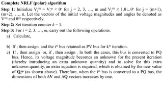
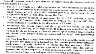
1.
UNIVERSITY OF GONDAR
Instituteof Technology
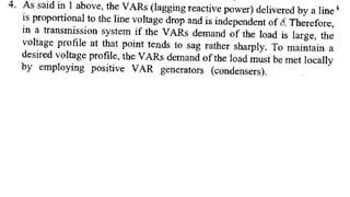
Department of Electrical and Computer Engineering
Computer Aided Power System Analysis(CAPA)
Chapter 2 Load/Power Flow Analysis
By Dawit Adane
2.
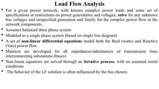
Load Flow Analysis
For a given power network, with known complex power loads and some set of
specifications or restrictions on power generations and voltages, solve for any unknown
bus voltages and unspecified generation and finally for the complex power flow in the
network components.
Assumes balanced three phase system
Modeled as a single phase system (based on single line diagram)
A set of non-linear differential equations model both the Real (watts) and Reactive
(Vars) power flow
Matrices are developed for all impedances/admittances of transmission lines
interconnecting substations (buses)
Non-linear equations are solved through an iterative process, with an assumed initial
conditions
The behavior of the LF solution is often influenced by the bus chosen.
3.
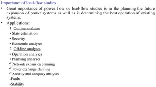
Importance of load-flowstudies
• Great importance of power flow or load-flow studies is in the planning the future
expansion of power systems as well as in determining the best operation of existing
systems.
• Applications:
1. On-line analyses
• State estimation
• Security
• Economic analyses
2. Off-line analyses
• Operation analyses
• Planning analyses
Network expansion planning
Power exchange planning
Security and adequacy analyses
-Faults
-Stability
4.
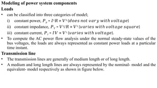
Modeling of powersystem components
Loads
• can be classified into three categories of model;
i) constant power, 𝑃𝑝 = 𝐼2
𝑅 ∝ 𝑉0
( )
𝑑𝑜𝑒𝑠 𝑛𝑜𝑡 𝑣𝑎𝑟𝑦 𝑤𝑖𝑡ℎ 𝑣𝑜𝑙𝑡𝑎𝑔𝑒
ii) constant impedance, 𝑃𝑌 = 𝑉2
/𝑅 ∝ 𝑉2
( )
𝑣𝑎𝑟𝑖𝑒𝑠 𝑤𝑖𝑡ℎ 𝑣𝑜𝑙𝑡𝑎𝑔𝑒 𝑠𝑞𝑢𝑎𝑟𝑒
iii) constant current, 𝑃𝐼 = 𝐼𝑉 ∝ 𝑉1
( ).
𝑣𝑎𝑟𝑖𝑒𝑠 𝑤𝑖𝑡ℎ 𝑣𝑜𝑙𝑡𝑎𝑔𝑒
• To compute the AC power flow analysis under the normal steady-state values of the
bus voltages, the loads are always represented as constant power loads at a particular
time instant.
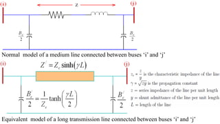
Transmission line
• The transmission lines are generally of medium length or of long length.
• A medium and long length lines are always represented by the nominal- model and the
equivalent- model respectively as shown in figure below.
5.
Normal model ofa medium line connected between buses ‘i’ and ‘j’
Equivalent model of a long transmission line connected between buses ‘i’ and ‘j’
6.
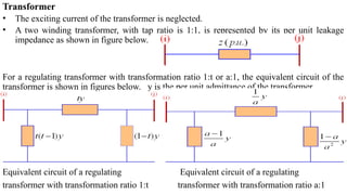
Transformer
• The excitingcurrent of the transformer is neglected.
• A two winding transformer, with tap ratio is 1:1, is represented by its per unit leakage
impedance as shown in figure below.
For a regulating transformer with transformation ratio 1:t or a:1, the equivalent circuit of the
transformer is shown in figures below. y is the per unit admittance of the transformer.
Equivalent circuit of a regulating Equivalent circuit of a regulating
transformer with transformation ratio 1:t transformer with transformation ratio a:1
7.
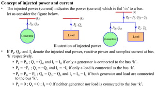
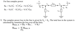
Concept of injectedpower and current
• The injected power (current) indicates the power (current) which is fed ‘in’ to a bus.
let us consider the figure below.
Illustration of injected power
• If Pk, Qk, and Ik denote the injected real power, reactive power and complex current at bus
‘k’ respectively,
• Pk = PG ; Qk = QG and Ik = IG if only a generator is connected to the bus ‘k’.
• Pk = −PL ; Qk = −QL and Ik = −IL if only a load is connected to the bus ‘k’.
• Pk = PG − PL ; Qk = QG − QL and Ik = IG − IL if both generator and load are connected
to the bus ‘k’.
• Pk = 0 ; Qk = 0 ; Ik = 0 If neither generator nor load is connected to the bus ‘k’.
9.
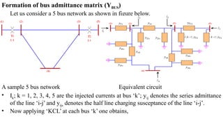
Formation of busadmittance matrix (YBUS)
Let us consider a 5 bus network as shown in figure below.
A sample 5 bus network Equivalent circuit
• Ik; k = 1, 2, 3, 4, 5 are the injected currents at bus ‘k’; yij denotes the series admittance
of the line ‘i-j’ and yijs denotes the half line charging susceptance of the line ‘i-j’.
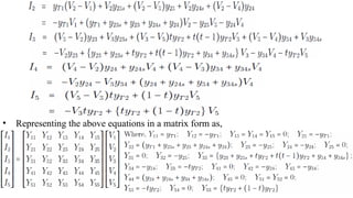
• Now applying ‘KCL’ at each bus ‘k’ one obtains,
• The matrixequation can be written as,
Where,
IBUS = [I1, I2, …, I5]T
(5 × 1) is the vector of bus injection currents
VBUS = [V1, V2, …, V5]T
(5 × 1) is the vector of bus voltages measured with respect
to the ground
YBUS (5 × 5) is the bus admittance matrix
• From the elements of the YBUS it can be observed that for i = 1, 2, …, 5;
Yii = sum total of all the admittances connected at bus ‘i’ called Self driving
admittance – diagonal elements
Yij = negative of the admittance connected between bus ‘i’ & ‘j’ (if these two buses are
physically connected with each other) called Mutual driving admittance – off-diagonal
element
Yij = 0; if there is no physical connection between buses ‘i’ and ‘j’
12.
• Similarly, fora ‘n’ bus power system, where,
IBUS = [I1, I2, …, In]T
(n × 1) is the vector of bus injection currents
VBUS = [V1, V2, …, Vn]T
(n × 1) is the vector of bus voltages
YBUS (n × n) is the bus admittance matrix
Read about the Formation of YBUS matrix in the presence of mutually coupled elements
Basic Power Flow Equation
• For a ‘n’ bus system,
Or,
• Complex power injected at bus ‘i’ is given by,
Now, ; ;
13.
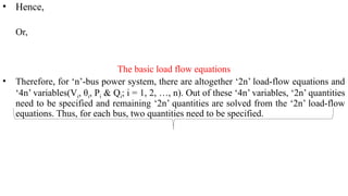
• Hence,
Or,
The basicload flow equations
• Therefore, for ‘n’-bus power system, there are altogether ‘2n’ load-flow equations and
‘4n’ variables(Vi, θi, Pi & Qi; i = 1, 2, …, n). Out of these ‘4n’ variables, ‘2n’ quantities
need to be specified and remaining ‘2n’ quantities are solved from the ‘2n’ load-flow
equations. Thus, for each bus, two quantities need to be specified.
14.
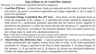
Type of Busesin AC Load Flow Analysis
The buses in a system are classified into three categories;
1. Load Bus (PQ bus) – At these buses, loads are connected and the values of loads (real, Pi,
and reactive, Qi, power ) are known (specified) and voltage magnitude, Vi & it’s angle, θi
need to be calculated.
2. Generator/Voltage Controlled/ Bus (PV bus) – these buses are the generator buses at
which the magnitude of the voltage, Vi, is specified and is kept constant by adjusting the
field current of a synchronous generator (provided that the reactive power supplied or
absorbed by the generator is within the limits) and also the real power, Pi, supplied by the
generator is also known according to the economic dispatch. Thus, the reactive power, Qi,
and voltage angle, θi, need to be calculated (unknown).
Note: Certain buses without generators may have voltage control capability; such buses are also designated
voltage-controlled buses at which the real power generation is simply zero.
3. Slack/Swing/ Bus (Reference bus) – a special generator bus serving as a reference for
voltage measurement and supplies system losses plus its share of the loads (generation
mismatch). Its voltage is specified to be fixed in both magnitude, Vi, & phase (angle), θi,
(for instance, 1∟00
pu) and the real, Pi, & reactive, Qi, powers are calculated (unknown).
Usually, the largest generator in the system is designated as the slack bus.
15.
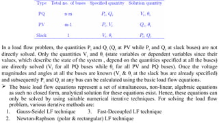
In a loadflow problem, the quantities Pi and Qi (Qi at PV while Pi and Qi at slack buses) are not
directly solved. Only the quantities Vi and θi (state variables or dependent variables since their
values, which describe the state of the system , depend on the quantities specified at all the buses)
are directly solved (Vi for all PQ buses while θi for all PV and PQ buses). Once the voltage
magnitudes and angles at all the buses are known (Vi & θi at the slack bus are already specified)
and subsequently Pi and Qi at any bus can be calculated using the basic load flow equations.
The basic load flow equations represent a set of simultaneous, non-linear, algebraic equations
as such no closed form, analytical solution for these equations exist. Hence, these equations can
only be solved by using suitable numerical iterative techniques. For solving the load flow
problem, various iterative methods are:
1. Gauss-Seidel LF technique 3. Fast-Decoupled LF technique
2. Newton-Raphson (polar & rectangular) LF technique
16.
Gauss Seidel LoadFlow Technique (GSLF)
• The injected current at bus ‘i’ of n-bus system is:
Hence,
• From the relation, we get,
Thus,
• This is the basic equation for performing GSLF.
𝐕𝐢=
𝟏
𝐘𝐢𝐢 [𝐏𝐢 − 𝐣𝐐𝐢
𝐕𝐢
∗
− ∑
𝐤=𝟏,≠𝐢
𝐧
𝐘𝐢𝐤 𝐕𝐤
]
17.
Initialization and StoppingCriteria
Initialization of the Voltage
All the unknown bus voltage are initialized to 1.0∟00
p.u (i.e., Vj
(0)
= 1.0∟00
for j = 2, 3, …,
n). This process of initializing all bus voltage to 1.0∟00
pu is called flat voltage start (because
of the uniform voltage profile assumed). V2
(0)
= V3
(0)
= … =Vn
(0)
= 1.0∟00
= 1.0 + j0
Stopping Criteria (Convergence)
The iterative process must be continued until either
1. The iteration count reached maximum iteration count number limit, NUM = NUMmax
2. The magnitude of change of bus voltage between two consecutive iteration is less than or
equal to a certain tolerance limit, ε for all bus voltages.
max|Vi
(k+1)
V
‒ i
(k)
| ≤ ε; i = 2, 3, …, n.
Ɐ
Acceleration of convergence
The number of iterations can be reduced if the iteration at each bus is accelerated, by
multiplying with a constant α, called the acceleration factor. In the (k+1)st
iteration we can let
where α is a real number b/n 1 < < 2. α is taken between 1.2 to 1.6, for GS load flow
ɑ
procedure.
18.
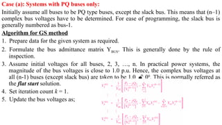
Case (a): Systemswith PQ buses only:
Initially assume all buses to be PQ type buses, except the slack bus. This means that (n–1)
complex bus voltages have to be determined. For ease of programming, the slack bus is
generally numbered as bus-1.
Algorithm for GS method
1. Prepare data for the given system as required.
2. Formulate the bus admittance matrix YBUS. This is generally done by the rule of
inspection.
3. Assume initial voltages for all buses, 2, 3, …, n. In practical power systems, the
magnitude of the bus voltages is close to 1.0 p.u. Hence, the complex bus voltages at
all (n-1) buses (except slack bus) are taken to be 1.0 00
. This is normally referred as
the flat start solution.
4. Set iteration count k = 1.
5. Update the bus voltages as;
19.
Or, in any(k + 1)st
iteration, the voltages are given by
Here note that when computation is carried out for bus-i, updated values are already
available for buses 2,3, …, (i-1) in the current (k+1)st
iteration. Hence these values are
used. For buses (i+1), ..., n, values from previous, kth
iteration are used.
6. Continue iterations till
Where, ε is the tolerance limit. Generally, it is customary to use a value of 0.0001 pu.
7. Compute slack bus power after voltages have converged. [assuming bus 1 is slack bus].
8. Compute all line flows as follow:
For line currents
20.
For line complexpower
9. The complex power loss in the line is given by Sik + Ski. The total loss in the system is
calculated by summing the loss over all the lines.
21.
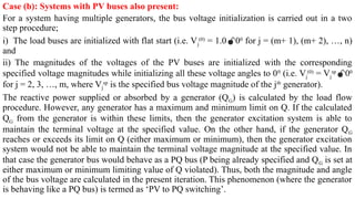
Case (b): Systemswith PV buses also present:
For a system having multiple generators, the bus voltage initialization is carried out in a two
step procedure;
i) The load buses are initialized with flat start (i.e. Vj
(0)
= 1.000
for j = (m+ 1), (m+ 2), …, n)
and
ii) The magnitudes of the voltages of the PV buses are initialized with the corresponding
specified voltage magnitudes while initializing all these voltage angles to 00
(i.e. Vj
(0)
= Vj
sp
00
for j = 2, 3, …, m, where Vj
sp
is the specified bus voltage magnitude of the jth
generator).
The reactive power supplied or absorbed by a generator (QG) is calculated by the load flow
procedure. However, any generator has a maximum and minimum limit on Q. If the calculated
QG from the generator is within these limits, then the generator excitation system is able to
maintain the terminal voltage at the specified value. On the other hand, if the generator QG
reaches or exceeds its limit on Q (either maximum or minimum), then the generator excitation
system would not be able to maintain the terminal voltage magnitude at the specified value. In
that case the generator bus would behave as a PQ bus (P being already specified and QG is set at
either maximum or minimum limiting value of Q violated). Thus, both the magnitude and angle
of the bus voltage are calculated in the present iteration. This phenomenon (where the generator
is behaving like a PQ bus) is termed as ‘PV to PQ switching’.
22.
Complete GSLF algorithm
Step1: Initialize Vj
(0)
= Vj
sp
00
for j = 2, 3, …, m and Vj
(0)
= 1.000
for j = (m+ 1), (m+ 2), …,
n. Set iteration count k = 1.
Step 2: For PV buses, i = 2, 3, …, m, carry out the following operations.
a) Calculate,
or
b) If, Qi
min
≤ Qi
(k)
≤ Qi
max
; then assign |Vi
(k)
| = Vi
sp
and θi
(k)
= (Ai
(k)
). The quantity Ai
(k)
is given
by,
c) If Qi
(k)
≥ Qi
max
, then set Qi
(k)
= Qi
max
and calculate
23.
d) If Qi
(k)
≤Qi
min
, then set Qi
(k)
= Qi
min
and calculate
Step 3: For PQ buses, i = (m+ 1), …, n, calculate
Step 4: Compute ei
(k)
= |Vi
(k)
− Vi
(k-1)
| for all i = 2,3, …, n;
Step 5: Compute e(k)
= max(e2
(k)
, e3
(k)
, …, en
(k)
);
Step 6: If e(k)
≤ ε, stop and print the solution. Else set k = k + 1 and go to step 2.
24.
Basic Newton -Raphson (NR) Techniques
Let there be ‘n’ equations in ‘n’ unknown variables x1, x2, …, xn as given below,
The quantities b1, b2, …, bn as well as the
functions f1, f2, …, fn are known.
To solve the above equations, first we take an initial guess of the solution and let the
vector of initial guesses be denoted as . Subsequently, first order Taylor’s series expansion
(neglecting the higher order terms) is carried out for these equation around the initial
guess of solution as follow:
25.
The above Equationscan be written in matrix form as,
In the above equation, the matrix containing the partial derivative terms is known as the
Jacobin matrix (J). It is an n x n square matrix.
By rearranging and simplifying the above equation yields
This is the basic equation for solving the ‘n’ algebraic equations given at first place.
26.
The steps ofsolution are as follow:
Step 1: Assume a vector of initial guess x(0)
and set iteration counter k = 0.
Step 2: Compute f1(x(k)
), f2(x(k)
), …, fn(x(k)
).
Step 3: Compute ∆m1, ∆m2, …, ∆mn.
Step 4: Compute error = max [|∆m1|, |∆m2|, …, |∆mn|]
Step 5: If error ≤ ε (pre - specified tolerance), then the final solution vector is x(k)
and print
the results. Otherwise go to step 6.
Step 6: Form the Jacobin matrix analytically and evaluate it at x = x(k)
.
Step 7: Calculate the correction vector by using the above equation.
Step 8: Update the solution vector x(k+1)
= x(k)
+ ∆x and update k = k + 1 and go back to
step 2.
27.
Newton Raphson LoadFlow Technique (NRLF) in polar coordinates
For NRLF techniques, the starting equations are same as the basic load flow
equations:
Assume that in an ‘n’ bus, ‘m’ machine system, the first ‘m’ buses are the generator
buses with bus 1 being the slack bus. Therefore, the unknown quantities are; (total
‘n–1’ quantities) & (total ‘n-m’ quantities). Thus, the total number of unknown
quantities is n–1+n–m = 2n–m–1. The specified quantities are; (total ‘n–m’
quantities) and . Hence, the total number of specified quantities is also (2n–m–1).
Since the injection real and reactive Power at any bus are functions of θ and V and
can be written as for i = 2, 3, …, n and for i = (m + 1), (m + 2), …, n. Assuming
initial guesses of the bus voltage angles (θ(0)
) and the bus voltage magnitudes (V(0)
),
The Taylor’s series expansion of the basic load flow equations are
28.
In the aboveequation, the quantity Pi(θ(0)
, V(0)
). is the calculated value of Pi with initial
guessed vectors θ(0)
, V(0)
.and can be denoted as . Similarly, for Qi(θ(0)
, V(0)
) = . With this
notation, the above equation can be written as:
Where, and . Also note that the vectors ∆θ and Psp
are of dimension (n − 1) × 1 each and
the vectors ∆V and Qsp
are of dimension (n−m) × 1 each.
29.
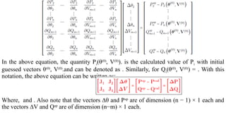
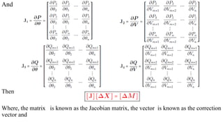
And
Then
Where, the matrixis known as the Jacobian matrix, the vector is known as the correction
vector and
30.
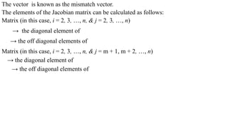
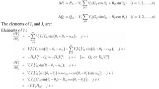
The vector isknown as the mismatch vector.
The elements of the Jacobian matrix can be calculated as follows:
Matrix (in this case, i = 2, 3, …, n, & j = 2, 3, …, n)
→ the diagonal element of
→ the off diagonal elements of
Matrix (in this case, i = 2, 3, …, n, & j = m + 1, m + 2, …, n)
→ the diagonal element of
→ the off diagonal elements of
31.
Matrix (in thiscase, i = m + 1, m + 2, …, n, & j = 2, 3, …, n)
→ the diagonal element of
→ the off diagonal elements of
Matrix (in this case, i = m + 1, m + 2, …, n, & j = m + 1, m + 2, …, n)
→the diagonal element of
→ the off diagonal elements of
Where, and
32.
Complete NRLF (polar)algorithm
Step 1: Initialize Vj
(0)
= Vj
sp
0
˂ o
for j = 2, 3, …, m and Vj
(0)
≤ 1.0∟0o
for j = (m+1),
(m+2), …, n. Let the vectors of the initial voltage magnitudes and angles be denoted as
V(0)
and θ(0)
respectively.
Step 2: Set iteration counter k = 1.
Step 3: For i = 2, 3, …, m, carry out the following operations.
a) Calculate,
b) If ; then assign and the ith
bus retained as PV bus for kth
iteration.
c) If , then assign or, if , then assign . In both the cases, this bus is converted to PQ
bus. Hence, its voltage magnitude becomes an unknown for the present iteration
(thereby introducing an extra unknown quantity) and to solve for this extra
unknown quantity, an extra equation is required, which is obtained by the new value
of Qi
sp
(as shown above). Therefore, when the ith
bus is converted to a PQ bus, the
dimensions of both ∆V and ∆Q vectors increases by one.
33.
In general, ifl generator buses (l ≤ (m− 1)) violate their corresponding reactive power
limits at step 3, then the dimensions of both ∆V and ∆Q vectors increases from (n – m)
to (n – m + l). However, the dimensions of both ∆P and ∆θ vectors remain the same.
Therefore, the size of matrix J2 becomes (n – 1) × (n – m + l), that of matrix J3
becomes (n – m + l) × (n – 1) and the matrix J4 becomes of size (n – m + l) × (n – m +
l). The size of matrix J1, however, does not change. Hence, the size of the matrix J
becomes (2n – m – 1 – l) × (2n – m – 1 – l) while the sizes of both the vectors ∆X and
∆M becomes (2n – m – 1 – l) × 1. Of course, if there is no generator reactive power
limit violation, then l = 0.
Step 4: Compute the vectors Pcal
and Qcal
with the vectors θ(k−1)
and V(k−1)
thereby forming the
vector ∆M. Let this vector be represented as ∆M = [∆M1, ∆M2, …, ∆M2n−m−1−l]T.
Step 5: Compute error = max (|∆M1|, |∆M2|, …, |∆M2n−m−1−l|).
Step 6: If error ≤ ε (pre - specified tolerance), then the final solution vectors are θ(k−1)
and
V(k−1)
and print the results. Otherwise go to step 7.
Step 7: Evaluate the Jacobian matrix with the vectors θ(k−1)
and V(k−1)
.
Step 8: Compute the correction vector ∆X.
Step 9: Update the solution vectors θ(k)
= θ(k−1)
+ ∆θ and V(k)
= V(k−1)
+ ∆V. Update k = k + 1
and go back to step 3.
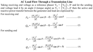
AC Load FlowThrough a Transmission Line
Taking receiving end voltage as a reference phasor VR = │VR│∟0o
and let the sending
end voltage lead it by an angle δ (torque angle) as VS = │VS│∟δo
then the active and
reactive power transfer between the generator and load are expressed by:
For receiving end
For sending end
36.
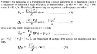
Normally, the resistanceof a transmission line is small compared to its reactance (since it
is necessary to maintain a high efficiency of transmission), so that θ = tan-1
X/Z ≈ 90o
;
where Z = R + jX. Therefore; the receiving end equations can be approximated as:
Since δ is very small, assuming cos δ ≈ 1 yields
Let │VS│ – │VR│= │∆V│, the magnitude of voltage drop across the transmission line,
then,
Fast Decoupled LFATechnique
The change in real power is primarily governed by the changes in the voltage angles, but
not in voltage magnitudes. On the other hand, the changes in the reactive power are
primarily influenced by the changes in voltage magnitudes, but not in the voltage angles.
(a) Under normal steady state operation, the voltage magnitudes are all nearly equal to
1.0.
(b) As the transmission lines are mostly reactive, the conductance's are quite small as
compared to the susceptance (Gij << Bij). Yij = Gij + Bij ; → lossless line (G is neglected)
(c) Under normal steady state operation the angular differences among the bus voltages
are quite small (θi − θj ≈ 0 (within 50
− 100
)).→cos θi − θj ≈ 1 & sin (θi − θj) ≈ (θi − θj) rad
≈ 0.
(d) The injected reactive power at any bus is always much less than the reactive power
consumed by the elements connected to this bus when these elements are shorted to the
ground (Qi << BiiVi
2
).
With these assumptions, the
equations for Jacobian elements
40.
Now, Gii andGij are quite small and negligible and also cos(θi−θj) ≈ 1 and sin(θi−θj) ≈ 0, as
[(θi−θj) ≈ 0]. Hence,
Similarly,
Again,
41.
The basic FDLFequation is:
Where,
is known as the correction vector and is the mismatch vector.
Thus, there is a decoupling between ‘∆P - ∆θ’ and ‘∆Q - ∆V’ relations (i.e., ∆P depends
only on ∆θ and ∆Q depends only on ∆V).
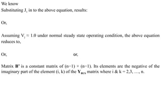
We know
Substituting J1in to the above equation, results:
Or,
Assuming Vj ≈ 1.0 under normal steady state operating condition, the above equation
reduces to,
Or, or,
Matrix B’ is a constant matrix of (n−1) × (n−1). Its elements are the negative of the
imaginary part of the element (i, k) of the YBUS matrix where i & k = 2,3, …, n.
45.
Similarly,
Or,
Matrix B” isa constant matrix of (n−m) × (n−m). Its elements are the negative of the
imaginary part of the element (i, k) of the YBUS matrix where i & k = m + 1, m + 2, …, n.
As the matrixes [B’] and [B”] are constant, the inverse of these matrices can be stored
only once and used in every iteration, thereby making the algorithm faster.
46.
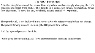
The “DC” PowerFlow
A further simplification of the power flow algorithm involves simply dropping the Q-V
equation altogether from FDLF. This results in a completely linear, noniterative, power
flow algorithm. To carry this out, we simply assume that all = 1.0 per unit.
The quantity ∆θ1 is not included in the vector ∆θ as the reference angle does not change.
The power flowing on each line using the DC power flow is then:
And the injected power at bus i is:
- Only good for calculating MW flows on transmission lines and transformers.
47.
Example: Consider thecircuit shown in Figure below. Using the data given below, use
fast decoupled power flow to find , , and │ │.
48.
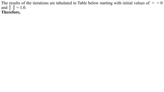
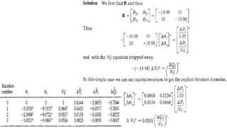
The results ofthe iterations are tabulated in Table below starting with initial values of = = 0
and │ │ = 1.0.
Therefore,
• The basicinformation contained in the load-flow output is:
i) All bus voltage magnitudes and phase angles w.r.t the slack bus.
ii) All bus active and reactive power injections.
iii) All line sending- and receiving-end complex power flows.
iv) Individual line losses can be deduced by subtracting receiving-end complex power
from sending-end complex power.
v) Total system losses can be deduced by summing item iv) for all lines, or by summing
complex power at all loads and generators and subtracting the totals.
• The most important information obtained from the load-flow is the system voltage
profile.
Need of Load Flow Study:
Designing a power system
Planning a power system
Expansion of power system
Providing guidelines for optimum operation of power system
Providing guidelines for various power system studies
51.
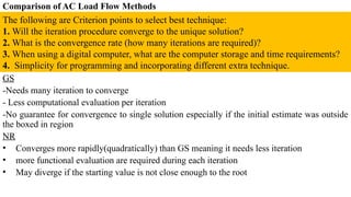
Comparison of ACLoad Flow Methods
GS
-Needs many iteration to converge
- Less computational evaluation per iteration
-No guarantee for convergence to single solution especially if the initial estimate was outside
the boxed in region
NR
• Converges more rapidly(quadratically) than GS meaning it needs less iteration
• more functional evaluation are required during each iteration
• May diverge if the starting value is not close enough to the root
The following are Criterion points to select best technique:
1. Will the iteration procedure converge to the unique solution?
2. What is the convergence rate (how many iterations are required)?
3. When using a digital computer, what are the computer storage and time requirements?
4. Simplicity for programming and incorporating different extra technique.
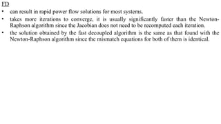
52.
FD
• can resultin rapid power flow solutions for most systems.
• takes more iterations to converge, it is usually significantly faster than the Newton-
Raphson algorithm since the Jacobian does not need to be recomputed each iteration.
• the solution obtained by the fast decoupled algorithm is the same as that found with the
Newton-Raphson algorithm since the mismatch equations for both of them is identical.
53.
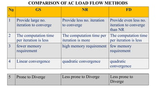
COMPARISON OF ACLOAD FLOW METHODS
No
.
GS NR FD
1 Provide large no.
iteration to converge
Provide less no. iteration
to converge
Provide even less no.
iteration to converge
than NR
2 The computation time
per iteration is less
The computation time per
iteration is more
The computation time
per iteration is less
3 fewer memory
requirement
high memory requirement few memory
requirement
4 Linear convergence quadratic convergence quadratic
convergence
5 Prone to Diverge Less prone to Diverge Less prone to
Diverge
Sparsity Techniques, TriangularFactorization and Optimal Ordering
• Consider a set of linear algebraic equations (in terms of real or complex variables).
Ax = b
• In general, efficient solution techniques depend on the structure and properties of the matrix
A. The properties of matrix A depend on the physical system or engineering problem
represented by matrix A. In general, matrices A resulting from power system analysis
problems have the following properties:
(a) they are of large dimension,
(b) they are sparse, i.e. many entries of the matrix are zero,
(c) they are topological symmetric (i.e., if the entry aij is nonzero, so is the entry aji)
(d) they are diagonal dominant (i.e. the diagonal element is absolutely greater than any
other entry in a row).
• Consider an electric power network consisting of n buses, ℓ branches, and m voltage
controlled buses. For this system, the dimension and approximate number of nonzero
elements in the admittance matrix and the Jacobian matrix (appearing in the
Newton/Raphson power flow) will be shown as in Table below 1.
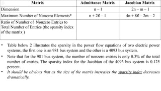
58.
D
• Table below2 illustrates the sparsity in the power flow equations of two electric power
systems, the first one is an 981 bus system and the other is a 4093 bus system.
• Note that for the 981 bus system, the number of nonzero entries is only 0.3% of the total
number of entries. The sparsity index for the Jacobian of the 4093 bus system is 0.125
percent.
• It should be obvious that as the size of the matrix increases the sparsity index decreases
dramatically.
Matrix Admittance Matrix Jacobian Matrix
Dimension n – 1 2n – m – 1
Maximum Number of Nonzero Elements* n + 2ℓ – 1 4n + 8ℓ – 2m – 2
Ratio of Number of Nonzero Entries to
Total Number of Entries (the sparsity index
of the matrix )
59.
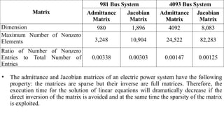
• The admittanceand Jacobian matrices of an electric power system have the following
property: the matrices are sparse but their inverse are full matrices. Therefore, the
execution time for the solution of linear equations will dramatically decrease if the
direct inversion of the matrix is avoided and at the same time the sparsity of the matrix
is exploited.
Matrix
981 Bus System 4093 Bus System
Admittance
Matrix
Jacobian
Matrix
Admittance
Matrix
Jacobian
Matrix
Dimension 980 1,896 4092 8,083
Maximum Number of Nonzero
Elements 3,248 10,904 24,522 82,283
Ratio of Number of Nonzero
Entries to Total Number of
Entries
0.00338 0.00303 0.00147 0.00125
60.
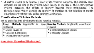
• A matrixis said to be sparse, if most of its elements are zero. The sparsity level
depends on the size of the system. Specifically, as the size of the electric power
system increases, the effects of sparsity become more pronounced. The
methodologies which exploit the sparsity of matrices in the solution of matrix
equations are collectively called sparsity techniques.
Classification of Solution Methods
can be classified into direct methods and iterative methods.
Read about Gaussian Elimination!
Direct Methods (applicable to linear
problems)
Iterative Methods (applicable to nonlinear
systems)
Matrix Inversion
Gaussian Elimination
Triangular Factorization
Coordinate (Gauss) Method
Conjugate Gradient
61.
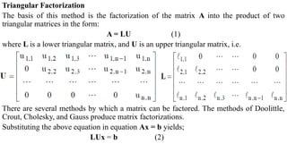
Triangular Factorization
The basisof this method is the factorization of the matrix A into the product of two
triangular matrices in the form:
A = LU (1)
where L is a lower triangular matrix, and U is an upper triangular matrix, i.e.
There are several methods by which a matrix can be factored. The methods of Doolittle,
Crout, Cholesky, and Gauss produce matrix factorizations.
Substituting the above equation in equation Ax = b yields;
LUx = b (2)
62.
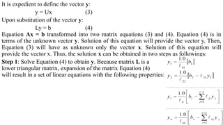
It is expedientto define the vector y:
y = Ux (3)
Upon substitution of the vector y:
Ly = b (4)
Equation Ax = b transformed into two matrix equations (3) and (4). Equation (4) is in
terms of the unknown vector y. Solution of this equation will provide the vector y. Then,
Equation (3) will have as unknown only the vector x. Solution of this equation will
provide the vector x. Thus, the solution x can be obtained in two steps as followings:
Step 1: Solve Equation (4) to obtain y. Because matrix L is a
lower triangular matrix, expansion of the matrix Equation (4)
will result in a set of linear equations with the following properties:
63.
Step 2: Sincethe vector y is now known, Equation (3) is
solved for the unknown vector x. Since the matrix U
is an upper triangular matrix, the solution will be obtained
with a series of substitutions as follows:
The solution of Equations (4) and (3) [steps 1 and 2,
respectively] are called forward substitution and
back substitution, respectively.
Example: Solve the matrix equation Ax = b using
forward and back substitutions. where
Assume that the matrix A has been factored
as follows:
64.
In summary, thesolution of a matrix equation Ax = b is easily obtained with a series of
substitutions (forward and back substitutions) if the matrix A can be factored into the
product of two triangular matrices (lower and upper). Thus, the solution procedure
involves three steps:
Step 1. Triangular Factorization
Step 2. Forward Substitution
Step 3. Back Substitution
Triangular Factorization Algorithms
A necessary condition for triangular factorization is that the matrix A is nonsingular.
Gaussian elimination provides a natural way of determining the triangular matrices L and
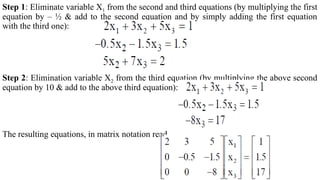
U. Consider the following matrix equation
2X1 + 3X2 + 5X3 = 1
X1 + X2 + X3 = 2
–2X1 + 2X2 + 2X3 = 1
An upper triangular matrix U can be obtained with the following steps:
65.
Step 1: Eliminatevariable X1 from the second and third equations (by multiplying the first
equation by – ½ & add to the second equation and by simply adding the first equation
with the third one):
Step 2: Elimination variable X2 from the third equation (by multiplying the above second
equation by 10 & add to the above third equation):
The resulting equations, in matrix notation read
66.
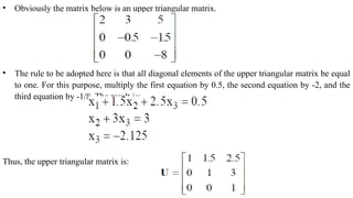
• Obviously thematrix below is an upper triangular matrix.
• The rule to be adopted here is that all diagonal elements of the upper triangular matrix be equal
to one. For this purpose, multiply the first equation by 0.5, the second equation by -2, and the
third equation by -1/8. The result is:
Thus, the upper triangular matrix is:
67.
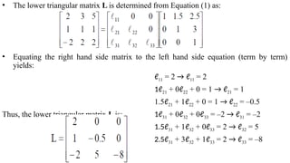
• The lowertriangular matrix L is determined from Equation (1) as:
• Equating the right hand side matrix to the left hand side equation (term by term)
yields:
ℓ11 = 2 → ℓ11 = 2
1ℓ21 + 0ℓ22 + 0 = 1 → ℓ21 = 1
1.5ℓ21 + 1ℓ22 + 0 = 1 → ℓ22 = –0.5
Thus, the lower triangular matrix L is: 1ℓ31 + 0ℓ32 + 0ℓ33 = –2 → ℓ31 = –2
1.5ℓ31 + 1ℓ32 + 0ℓ33 = 2 → ℓ32 = 5
2.5ℓ31 + 3ℓ32 + 1ℓ33 = 2 → ℓ33 = –8
68.
• The Gaussianelimination is performed in n steps, where n is the numbers of rows in the
matrix. Each step (for example, the step for row i) involves the following sub-steps:
Sub-step 1. Eliminate the ith
variable from the remaining rows of the matrix (i.e. rows
i+1,...,n) by performing row operations. Note that this sub-step must be omitted if the ith
row
is the last row of the matrix.
Sub-step 2. Multiply the ith
row of the matrix by the inverse of the diagonal element. The
resulting row i will have the diagonal element equal to 1.0.
• The above two sub-step procedure must be applied to all rows of the matrix sequentially
starting from row i. Upon completion of the procedure, the resulting matrix is the upper
triangular matrix U with all diagonal elements equal to 1.0.
• The lower triangular matrix L is obtained as follows: (a) The element ℓij of the matrix L for i
≥ j equals the entry ij of the modified matrix before the jth
step (i.e. step j-1) of the Gaussian
elimination procedure. (b) The element ℓij of the matrix L for i < j equals zero.
• In other words, the Gaussian elimination yields, as a by product, the triangular factorization
of the matrix. It is expedient to perform the described procedure in a tableau form in which
case the L and U matrices can be obtained by inspection of the final result. The procedure is
also called Gaussian elimination in tableau form.
69.
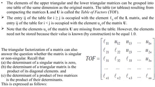
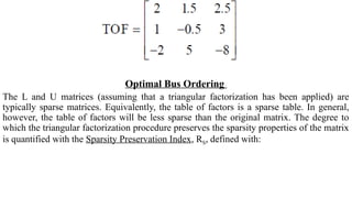
• The elementsof the upper triangular and the lower triangular matrices can be grouped into
one table of the same dimension as the original matrix. The table (or tableau) resulting from
compacting the matrices L and U is called the Table of Factors (TOF).
The entry ij of the table for i ≥ j is occupied with the element ℓij of the L matrix, and the
entry ij of the table for i < j is occupied with the element uij of the matrix U.
Note that the elements uii of the matrix U are missing from the table. However, the elements
need not be stored because their value is known (by construction) to be equal 1.0.
The triangular factorization of a matrix can also
answer the question whether the matrix is singular
or non-singular. Recall that
(a) the determinant of a singular matrix is zero,
(b) the determinant of a triangular matrix is the
product of its diagonal elements. and
(c) the determinant of a product of two matrices
is the product of their determinants.
This is expressed as follows:
70.
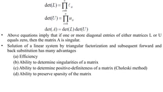
• Above equationsimply that if one or more diagonal entries of either matrices L or U
equals zero, then the matrix A is singular.
• Solution of a linear system by triangular factorization and subsequent forward and
back substitution has many advantages
(a) Efficiency
(b) Ability to determine singularities of a matrix
(c) Ability to determine positive-definiteness of a matrix (Choleski method)
(d) Ability to preserve sparsity of the matrix
Optimal Bus Ordering
TheL and U matrices (assuming that a triangular factorization has been applied) are
typically sparse matrices. Equivalently, the table of factors is a sparse table. In general,
however, the table of factors will be less sparse than the original matrix. The degree to
which the triangular factorization procedure preserves the sparsity properties of the matrix
is quantified with the Sparsity Preservation Index, RS, defined with:
73.
The sparsity preservationindex greatly affect or impact the amount of computer storage
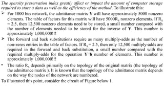
required to store a data as well as the efficiency of the method. To illustrate this:
For 1000 bus network, the admittance matrix Y will have approximately 5000 nonzero
elements. The table of factors for this matrix will have 5000RS nonzero elements. If RS
= 2.5, then 12,500 nonzero elements need to be stored, a small number compared with
the number of elements needed to be stored for the inverse of Y. This number is
approximately 1,000,000!!!
The forward and back substitutions require as many multiply-adds as the number of
non-zeros entries in the table of factors. If RS = 2.5, then only 12,500 multiply-adds are
required in the forward and back substitution, a small number compared with the
required multiply-adds for the operation Y-1
b number of elements. This number is
approximately 1,000,000!!!
• The ratio RS depends primarily on the topology of the original matrix (the topology of
the admittance matrix ). It is known that the topology of the admittance matrix depends
on the way the nodes of the network are numbered.
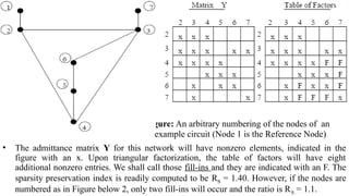
To illustrated this point, consider the circuit of Figure below 1.
74.
Figure: An arbitrarynumbering of the nodes of an
example circuit (Node 1 is the Reference Node)
• The admittance matrix Y for this network will have nonzero elements, indicated in the
figure with an x. Upon triangular factorization, the table of factors will have eight
additional nonzero entries. We shall call those fill-ins and they are indicated with an F. The
sparsity preservation index is readily computed to be RS = 1.40. However, if the nodes are
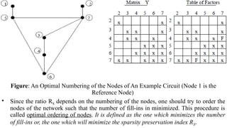
numbered as in Figure below 2, only two fill-ins will occur and the ratio is RS = 1.1.
75.
Figure: An OptimalNumbering of the Nodes of An Example Circuit (Node 1 is the
Reference Node)
• Since the ratio RS depends on the numbering of the nodes, one should try to order the
nodes of the network such that the number of fill-ins in minimized. This procedure is
called optimal ordering of nodes. It is defined as the one which minimizes the number
of fill-ins or, the one which will minimize the sparsity preservation index RS.
76.
• To findthe optimal ordering of the nodes of a network is very difficult, since the number
of possible numbering alternatives is n! (n factorial) is large. However, several efficient
near-optimal (sub-optimal) ordering schemes have been developed. In the early 60's, Bill
Tinney developed three schemes for near-optimal ordering which are known as Tinney
Schemes 1, 2, 3. These schemes are listed in increasing order of programming complexity,
execution time, and optimality.
Scheme 1: The nodes of a network are ordered in such a way that a lower numbered node
has less or equal number of adjacent branches than any higher numbered node.
Scheme 2: After ordering using scheme 1, Fill-ins are generated in pairs occupying symmetric
positions with respect to the diagonal. Thus, it may be assumed that a pair of fill-ins in
positions (i,j) and (j,i) corresponds to a fictitious branch between nodes i and j. Then the nodes
of the network are ordered in such a way that a lower numbered node has a less or equal
number of adjacent actual or fictitious branches than any higher numbered node.
Scheme 3: This scheme starts from an arbitrary numbering of the system nodes. Then the
near-optimally ordered nodes 1,2,..., are selected one at a time as follows. Assume that k
nodes have been optimally ordered, 1 through k, while the remaining nodes are arbitrarily
numbered k+1 through n. The next optimal number k+1 is assigned to the node which
generates the minimum number of fill-ins among all arbitrarily numbered nodes.
77.
• The performanceof these schemes on actual electric power networks indicates that
scheme 2 is much better than scheme 1 and scheme 3 is slightly better than scheme 2.
This means that if RS1, RS2, and RS3 are the resulting sparsity preservation indices with
the three ordering schemes, respectively, the following should be expected:
RS1 ≥ RS2 ≥ RS3
Example: Consider the electric power system of Figure below 1. Only the topology of the
network is indicated. The indicated numbering of the nodes is arbitrary. Bus 1 is assumed
to be the reference bus. Consider the sparsity properties of the admittance matrix.
a) Determine the optimal ordering of nodes according to scheme 1 and compute
the sparsity preservation index for the admittance matrix.
b) Determine the optimal ordering of nodes according to schemes 2 and compute
the sparsity preservation index for the admittance matrix.
Solution
(Part a):
• The number of circuits or branches each bus/node connected with is it degree of
connection.
• Note that circuits terminated to the reference bus are not counted.
78.
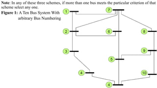
Note: In anyof these three schemes, if more than one bus meets the particular criterion of that
scheme select any one.
Figure 1: A Ten Bus System With
arbitrary Bus Numbering
79.
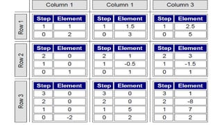
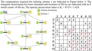
The computations requiredfor ordering scheme 1 are indicated in Figure below 2. The
triangular factorization has been simulated and locations of fill-ins are indicated with an F
which counts 14 fill-ins. The sparsity preservation index is RS = 47/33 = 1.424.
80.
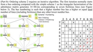
(Part b): Orderingscheme 2 requires an iterative algorithm. The first iteration normally starts
from a bus ordering computed with the simple scheme 1 as the triangular factorization of the
admittance matrix generates 14 fill-ins corresponding to seven fictitious lines (see Figure
below 3). The bus numbering is such that a higher number bus has a higher or equal total
number of lines (including fictitious) than any other lower number bus.
81.
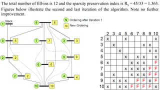
The total numberof fill-ins is 12 and the sparsity preservation index is RS = 45/33 = 1.363.
Figures below illustrate the second and last iteration of the algorithm. Note no further
improvement.
82.
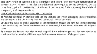
The only virtueof scheme 1 is its simplicity and speed. The improved performance of
scheme 2 over scheme 1 justifies the additional time required for its execution. On the
other hand, gains in performance of scheme 3 over scheme 2 do not justify its additional
complexity and execution time.
Near Optimal Schemes for Sparse Matrix Ordering.
1) Number the buses by starting with the one that has the fewest connected lines or branches
and ending with that bus having the most connected lines or branches.
2) Order the buses so that at each step of the elimination process the next bus to be eliminated
is the one having the fewest connected lines or branches, i.e. the fewest non-zero off-diagonal
terms.
3) Number the busses such that at each step of the elimination process the next row to be
eliminated is the one that will introduce the fewest new non-zero off-diagonal terms.
83.
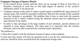
Computer Storage ofSparse Matrix
• In the normal power system network, there are an average of three to four lines or
branches connected to each bus so that high degree of sparsity in the system’s
admittance matrix Y are preserved.
• Computer storage of the entire Y matrix would require a prohibitively large amount of
storage space and would be extremely inefficient. However the storage of the essential
non-zero elements is acceptable. The problem then is how to store only the nonzero
elements of the Y matrix without losing the inherent column and row addressing of
each element in the matrix.
• In order to take advantage of the large number of zero elements, special schemes are
required to store sparse matrices. The main goal is to represent only the nonzero
elements, and to be able to perform the common matrix operations.
The problem is:
1) Store the A matrix with the minimum amount of space in the computer.
2) And since this matrix will later be operated on by a row-by-row elimination process,
each row should be easily recreated from the compressed storage state.
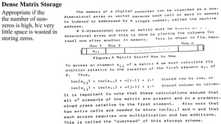
Storage Scheme 1:– is the so-called coordinate format w/c is the simplest storage scheme
• The data structure consists of three arrays:
(1) a real array containing all the real or complex values of the nonzero elements of
A in any order;
(2) an integer array containing their row indices; and
(3) a second integer array containing their column indices. All three arrays are of
length t, the number of nonzero elements.
Consider the 6 X 6 sparse matrix A
shown in figure below:
87.
Sparsity Techniques, TriangularFactorization and Optimal Ordering
• is advantageous for its simplicity and its flexibility.
Storage Scheme 2: – Compressed Sparse Row (CSR) format or/alternatively Compressed
Sparse Column (CSC) scheme.
• This scheme is preferred over the coordinate scheme because it is often more useful for
performing typical computations. On the other hand, the coordinate scheme is
advantageous for its simplicity and its flexibility.
• This scheme is obtained by alleviating the problem of repeating and redundant row index
numbers from the first scheme.
• This scheme requires two arrays of length t and one array of length c, giving a total of 2t +
c cells
88.
Gustavson’s Procedure toconstruct Storage Scheme 2:
All information present in the A matrix such as, values of the non-zero elements and their individual row and
column addresses are stored in three one-dimensional arrays.
1. The first array which will be labelled Value: begins with row one and proceeds row by row storing values
of all non-zero elements in order of appearance.
For the A matrix:
Value = 2, 1, 4, 3, 6, 3, 8, 5, 9, 1
• The dimension of Value is equal to the total number of nonzero terms in the matrix.
2. The second array is labelled Column index: it stores, with a one-to-one correspondence of the column
number of each element in the array Value.
Column index = 1, 4, 3, 1, 2, 6, 4, 1, 5, 6
• The dimension of Column index is equal to the dimension of Value.
3. The last array will be labelled Row start index: the first element in this array is always equal to one and
keeps running with the previous each row block begins and the total number of non zero elements in the
previous row.
RSI (1) = 1
RSI (2) = RSI (1) + the no. of non zero terms in row one
RSI (3) = RSI (2) + the no. of non zero terms in row two ….so on
89.
RSI = 1,3, 4, 7, 8, 10
The number of non-zero terms in the ith
row is:
RSI (i + 1) – RSI (i)
Procedures used to recreate any row from compressed storage:
• Let the value of RSI (i) = a and RSI (i + 1) = b. There are (b – a) non-zero terms in the ith
row.
• The ith
row begins at Value (a) in column CI (a), and ends at Value (b – 1) in column CI (b
– 1). These are the column numbers and values of the first and last non-zero elements in the
ith
row. If the value of CI (a) not equal to 1, zeroes are simply filled in all positions until CI
(a) is reached. The next non-zero term in the ith
row is Value (a + 1) in CI (a + 1). This
process continues until the entire ith
row is recreated in usable form.
Example
• Recreate the 3th
row of the A matrix from its compressed form in the three arrays VALUE,
CI and RSI.
The number of non-zero elements in row 3 is:
RSI (4) – RSI (3)
From the RSI array, 7 - 4 = 3
90.
• The firstnon-zero terms in row 3 is equal to:
Value (RSI (3)) = Value (4) = 3
It is in column position equal to CI (4) = 1
• The first part of this row is:
3 – – – – –
The next term is = Value (5) = 6,
in column position = CI (5) = 2,
• The second part of this row is:
3 6 – – – –
• The last term is = Value (6) = 3,
in column position = CI (6) = 6.
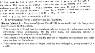
• Since there are only 3 significant elements in row 3 this process is completed and the
constructed row is:
3 6 0 0 0 3
91.
Storage Scheme 3:
•This scheme saves storage by packing each row and column index of the first scheme into
one cell using the following equation:
Nij = n x (i – 1) + j
• To retrieve or unpack the values of row i and column j, we use the following equations
Row i = [(Nij – 1)/n] + 1 Note: take only the integer part of the value.
Column j = Nij – [n x (i – 1)]
• This scheme requires only 2t cells but it involves more computation to pack and unpack the
indices.
Example: For matrix A
Value = 2, 1, 4, 3, 6, 3, 8, 5, 9, 1
Nij = 1, 4, 9, 13, 14, 18, 22, 25, 29, 36
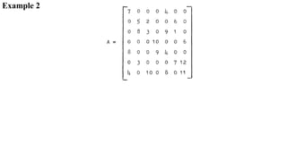
A.C.-D.C. LOAD FLOW
Thereare two approaches for load flow analysis of an AC system having one or two HVDC links.
These are:
a. Simultaneous solution technique
the equations pertaining to the A.C. system and the equations pertaining to the DC system are
solved together.
b. Sequential solution technique
the AC and DC systems are solved separately and the coupling between the AC and DC system
in accomplished by injecting an equivalent amount of real and reactive power at the terminal
AC buses.
For an HVDC link existing between buses ‘i’ and ‘j’ of an AC system (rectifier at bus ‘i’ and inverter at
bus ‘j’), the effect of the DC link is incorporated into the AC system by injections P(R)
DCi and Q(R)
DCi at
bus ‘i’ and P(I)
DCj and Q(I)
DCj at bus ’j’ (the super scripts ‘R’ and ‘I’ denote the rectifier and inverter
respectively). Therefore, the net injected power at bus ’i’ and ‘j’ are: Pi
Total
= PACi + P(R)
DCi; Qi
Total
= QACi +
Q(R)
DCi; Pj
Total
= PACj + P(I)
DCj; Qj
Total
= QACj + Q(I)
DCj. With these net injected powers, the AC system is
again solved and subsequently, the equivalent injected powers (P(R)
DCi, Q(R)
DCi, P(I)
DCj, Q(I)
DCi) and the total
injected powers (Pi
Total
, Qi
Total
, Pj
Total
, Qj
Total
) are updated. This process of alternately solving AC and DC
system quantities is continued till the changes in AC system and DC system quantities between two
consecutive iterations become less then a threshold value.
96.
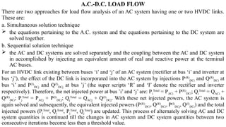
DC system model
Thebasic assumptions for deriving a suitable model of a HVDC system for steady state
operation:
a. The three phase AC voltages at the terminal bus bar are balanced and sinusoidal.
b. The converter operation is perfectly balanced.
c. The direct current and voltages are smooth.
d. The converter transformer is lossless and the magnetizing admittance is ignored.
The equivalent circuit of the converter (either rectifier or inverter) is shown in Figure
below.
97.
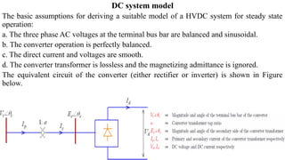
For rectifier
For inverter
‘N’= the number of six-pulse bridges at any particular side
‘Φ’ = the angular difference between the terminal voltages and primary current of the
transformer, i.e. the power factor of the converter as seen by the AC bus.
‘Xc’ = the commutating reactance of the converter transformer and
‘α’ and ‘γ’ = the firing angle of the rectifier and the extinction angle of the inverter
respectively.
VdO = No-load direct voltage for converters
The rectifier and the inverter are interconnected though the following equation:
Rd = the DC link resistance.
98.
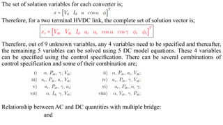
The set ofsolution variables for each converter is;
Therefore, for a two terminal HVDC link, the complete set of solution vector is;
Therefore, out of 9 unknown variables, any 4 variables need to be specified and thereafter,
the remaining 5 variables can be solved using 5 DC model equations. These 4 variables
can be specified using the control specification. There can be several combinations of
control specification and some of their combination are;
Relationship between AC and DC quantities with multiple bridge:
and
99.
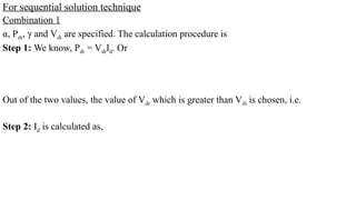
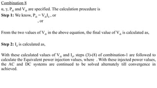
For sequential solutiontechnique
Combination 1
α, Pdr, γ and Vdi are specified. The calculation procedure is
Step 1: We know, Pdr = VdrId. Or
Out of the two values, the value of Vdr which is greater than Vdi is chosen, i.e.
Step 2: Id is calculated as,
100.
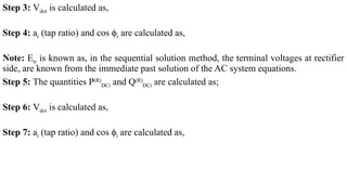
Step 3: Vdoris calculated as,
Step 4: ar (tap ratio) and cos ϕr are calculated as,
Note: Etr is known as, in the sequential solution method, the terminal voltages at rectifier
side, are known from the immediate past solution of the AC system equations.
Step 5: The quantities P(R)
DCi and Q(R)
DCi are calculated as;
Step 6: Vdoi is calculated as,
Step 7: ai (tap ratio) and cos ϕi are calculated as,
101.
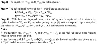
Step 8: Thequantities P(I)
DCj and Q(I)
DCj are calculated as;
Step 9: The net injected power at bus ‘i’ and ‘j’ are calculated as;
Pi
Total
= PACi + P(R)
DCi; Qi
Total
= QACi + Q(R)
DCi
Pj
Total
= PACj + P(I)
DCj; Qj
Total
= QACj + Q(I)
DCj
Step 10: With these net injected powers, the AC system is again solved to obtain the
updated values of Etr and Eti and subsequently, steps (1) - (8) are repeated again to update
the values of P(R)
DCi, Q(R)
DCi, P(I)
DCj and Q(I)
DCj till convergence in obtained.
Note:
At the rectifier end, P(R)
DCi = P
‒ dr and Q(R)
DCi = Q
‒ dr as the rectifier draws both real and
reactive power from the grid.
At the inverter end, P(I)
DCj = Pdi and Q(I)
DCj = Q
‒ di as the inverter supplies real power to the
AC grid and draws reactive power from the AC grid.
102.
Combination 8
α, γ,Pdi and Vdr are specified. The calculation procedure is
Step 1: We know, Pdi = VdiId , or
, or
From the two values of Vdi in the above equation, the final value of Vdi is calculated as,
Step 2: Id is calculated as,
With these calculated values of Vdi and Id, steps (3)-(8) of combination-1 are followed to
calculate the Equivalent power injection values, where . With these injected power values,
the AC and DC systems are continued to be solved alternately till convergence in
achieved.
103.
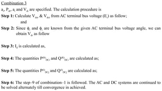
Combination 3
ar, Pdr,ai and Vdi are specified. The calculation procedure is
Step 1: Calculate Vdor & Vdoi from AC terminal bus voltage (Et) as follow;
and
Step 2: Since ϕr and ϕi are known from the given AC terminal bus voltage angle, we can
obtain Vdr as follow
Step 3: Id is calculated as,
Step 4: The quantities P(R)
DCi and Q(R)
DCi are calculated as;
Step 5: The quantities P(I)
DCj and Q(I)
DCj are calculated as;
Step 6: The step–9 of combination–1 is followed. The AC and DC systems are continued to
be solved alternately till convergence in achieved.
104.
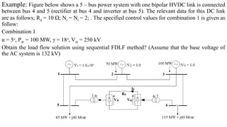
Example: Figure belowshows a 5 – bus power system with one bipolar HVDC link is connected
between bus 4 and 5 (rectifier at bus 4 and inverter at bus 5). The relevant data for this DC link
are as follows; Rd = 10 Ω; Nr = Ni = 2; . The specified control values for combination 1 is given as
follow:
Combination 1
α = 5o
, Pdr = 100 MW, γ = 18o
, Vdi = 250 kV
Obtain the load flow solution using sequential FDLF method? (Assume that the base voltage of
the AC system is 132 kV)
105.
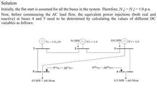
Solution
Initially, the flatstart is assumed for all the buses in the system. Therefore, |V4| = |V5| = 1.0 p.u.
Now, before commencing the AC load flow, the equivalent power injections (both real and
reactive) at buses 4 and 5 need to be determined by calculating the values of different DC
variables as follows:
COMPARISON OF ACLOAD FLOW METHODS
GS
-Needs many iteration
-No guarantee for convergence to single solution especially if the initial estimate
was outside the boxed in region
NR
Converges more rapidly(quadratically) than GS meaning it needs less iteration
However, more functional evaluation are required during each iteration
May diverge if the starting value is not close enough to the root
The following questions are Criterion:
1. Will the iteration procedure converge to the
unique solution?
2. What is the convergence rate (how many
iterations are required)?
3. When using a digital computer, what are the
computer storage and time requirements?
4. Simplicity for programming and incorporating
different extra technique.
109.
COMPARISON OF LOADFLOW METHODS
No. GS NR FD
1 Provide large no.
iteration to converge
Provide less no. iteration
to converge
Provide even less no.
iteration to converge
than NR
2 The computation time
per iteration is less
The computation time per
iteration is more
The computation time
per iteration is less
3 fewer memory
requirement
high memory requirement few memory
requirement
4 Linear convergence quadratic convergence quadratic
convergence
5 Prone to Diverge Less prone to Diverge Less prone to Diverge


![• The matrix equation can be written as,
Where,
IBUS = [I1, I2, …, I5]T
(5 × 1) is the vector of bus injection currents
VBUS = [V1, V2, …, V5]T
(5 × 1) is the vector of bus voltages measured with respect
to the ground
YBUS (5 × 5) is the bus admittance matrix
• From the elements of the YBUS it can be observed that for i = 1, 2, …, 5;
Yii = sum total of all the admittances connected at bus ‘i’ called Self driving
admittance – diagonal elements
Yij = negative of the admittance connected between bus ‘i’ & ‘j’ (if these two buses are
physically connected with each other) called Mutual driving admittance – off-diagonal
element
Yij = 0; if there is no physical connection between buses ‘i’ and ‘j’](https://image.slidesharecdn.com/powersystemiichapter-2loadorpowerflowanalysis-250307130912-a5e83562/85/Power-system-II-Chapter-2-Load-or-power-flow-analysis-pptx-11-320.jpg)
![• Similarly, for a ‘n’ bus power system, where,
IBUS = [I1, I2, …, In]T
(n × 1) is the vector of bus injection currents
VBUS = [V1, V2, …, Vn]T
(n × 1) is the vector of bus voltages
YBUS (n × n) is the bus admittance matrix
Read about the Formation of YBUS matrix in the presence of mutually coupled elements
Basic Power Flow Equation
• For a ‘n’ bus system,
Or,
• Complex power injected at bus ‘i’ is given by,
Now, ; ;](https://image.slidesharecdn.com/powersystemiichapter-2loadorpowerflowanalysis-250307130912-a5e83562/85/Power-system-II-Chapter-2-Load-or-power-flow-analysis-pptx-12-320.jpg)
![Gauss Seidel Load Flow Technique (GSLF)
• The injected current at bus ‘i’ of n-bus system is:
Hence,
• From the relation, we get,
Thus,
• This is the basic equation for performing GSLF.
𝐕𝐢=
𝟏
𝐘𝐢𝐢 [𝐏𝐢 − 𝐣𝐐𝐢
𝐕𝐢
∗
− ∑
𝐤=𝟏,≠𝐢
𝐧
𝐘𝐢𝐤 𝐕𝐤
]](https://image.slidesharecdn.com/powersystemiichapter-2loadorpowerflowanalysis-250307130912-a5e83562/85/Power-system-II-Chapter-2-Load-or-power-flow-analysis-pptx-16-320.jpg)
![Or, in any (k + 1)st
iteration, the voltages are given by
Here note that when computation is carried out for bus-i, updated values are already
available for buses 2,3, …, (i-1) in the current (k+1)st
iteration. Hence these values are
used. For buses (i+1), ..., n, values from previous, kth
iteration are used.
6. Continue iterations till
Where, ε is the tolerance limit. Generally, it is customary to use a value of 0.0001 pu.
7. Compute slack bus power after voltages have converged. [assuming bus 1 is slack bus].
8. Compute all line flows as follow:
For line currents](https://image.slidesharecdn.com/powersystemiichapter-2loadorpowerflowanalysis-250307130912-a5e83562/85/Power-system-II-Chapter-2-Load-or-power-flow-analysis-pptx-19-320.jpg)
![The steps of solution are as follow:
Step 1: Assume a vector of initial guess x(0)
and set iteration counter k = 0.
Step 2: Compute f1(x(k)
), f2(x(k)
), …, fn(x(k)
).
Step 3: Compute ∆m1, ∆m2, …, ∆mn.
Step 4: Compute error = max [|∆m1|, |∆m2|, …, |∆mn|]
Step 5: If error ≤ ε (pre - specified tolerance), then the final solution vector is x(k)
and print
the results. Otherwise go to step 6.
Step 6: Form the Jacobin matrix analytically and evaluate it at x = x(k)
.
Step 7: Calculate the correction vector by using the above equation.
Step 8: Update the solution vector x(k+1)
= x(k)
+ ∆x and update k = k + 1 and go back to
step 2.](https://image.slidesharecdn.com/powersystemiichapter-2loadorpowerflowanalysis-250307130912-a5e83562/85/Power-system-II-Chapter-2-Load-or-power-flow-analysis-pptx-26-320.jpg)
![In general, if l generator buses (l ≤ (m− 1)) violate their corresponding reactive power
limits at step 3, then the dimensions of both ∆V and ∆Q vectors increases from (n – m)
to (n – m + l). However, the dimensions of both ∆P and ∆θ vectors remain the same.
Therefore, the size of matrix J2 becomes (n – 1) × (n – m + l), that of matrix J3
becomes (n – m + l) × (n – 1) and the matrix J4 becomes of size (n – m + l) × (n – m +
l). The size of matrix J1, however, does not change. Hence, the size of the matrix J
becomes (2n – m – 1 – l) × (2n – m – 1 – l) while the sizes of both the vectors ∆X and
∆M becomes (2n – m – 1 – l) × 1. Of course, if there is no generator reactive power
limit violation, then l = 0.
Step 4: Compute the vectors Pcal
and Qcal
with the vectors θ(k−1)
and V(k−1)
thereby forming the
vector ∆M. Let this vector be represented as ∆M = [∆M1, ∆M2, …, ∆M2n−m−1−l]T.
Step 5: Compute error = max (|∆M1|, |∆M2|, …, |∆M2n−m−1−l|).
Step 6: If error ≤ ε (pre - specified tolerance), then the final solution vectors are θ(k−1)
and
V(k−1)
and print the results. Otherwise go to step 7.
Step 7: Evaluate the Jacobian matrix with the vectors θ(k−1)
and V(k−1)
.
Step 8: Compute the correction vector ∆X.
Step 9: Update the solution vectors θ(k)
= θ(k−1)
+ ∆θ and V(k)
= V(k−1)
+ ∆V. Update k = k + 1
and go back to step 3.](https://image.slidesharecdn.com/powersystemiichapter-2loadorpowerflowanalysis-250307130912-a5e83562/85/Power-system-II-Chapter-2-Load-or-power-flow-analysis-pptx-33-320.jpg)
![Now, Gii and Gij are quite small and negligible and also cos(θi−θj) ≈ 1 and sin(θi−θj) ≈ 0, as
[(θi−θj) ≈ 0]. Hence,
Similarly,
Again,](https://image.slidesharecdn.com/powersystemiichapter-2loadorpowerflowanalysis-250307130912-a5e83562/85/Power-system-II-Chapter-2-Load-or-power-flow-analysis-pptx-40-320.jpg)
![Similarly,
Or,
Matrix B” is a constant matrix of (n−m) × (n−m). Its elements are the negative of the
imaginary part of the element (i, k) of the YBUS matrix where i & k = m + 1, m + 2, …, n.
As the matrixes [B’] and [B”] are constant, the inverse of these matrices can be stored
only once and used in every iteration, thereby making the algorithm faster.](https://image.slidesharecdn.com/powersystemiichapter-2loadorpowerflowanalysis-250307130912-a5e83562/85/Power-system-II-Chapter-2-Load-or-power-flow-analysis-pptx-45-320.jpg)


![Step 2: Since the vector y is now known, Equation (3) is
solved for the unknown vector x. Since the matrix U
is an upper triangular matrix, the solution will be obtained
with a series of substitutions as follows:
The solution of Equations (4) and (3) [steps 1 and 2,
respectively] are called forward substitution and
back substitution, respectively.
Example: Solve the matrix equation Ax = b using
forward and back substitutions. where
Assume that the matrix A has been factored
as follows:](https://image.slidesharecdn.com/powersystemiichapter-2loadorpowerflowanalysis-250307130912-a5e83562/85/Power-system-II-Chapter-2-Load-or-power-flow-analysis-pptx-63-320.jpg)

![Storage Scheme 3:
• This scheme saves storage by packing each row and column index of the first scheme into
one cell using the following equation:
Nij = n x (i – 1) + j
• To retrieve or unpack the values of row i and column j, we use the following equations
Row i = [(Nij – 1)/n] + 1 Note: take only the integer part of the value.
Column j = Nij – [n x (i – 1)]
• This scheme requires only 2t cells but it involves more computation to pack and unpack the
indices.
Example: For matrix A
Value = 2, 1, 4, 3, 6, 3, 8, 5, 9, 1
Nij = 1, 4, 9, 13, 14, 18, 22, 25, 29, 36](https://image.slidesharecdn.com/powersystemiichapter-2loadorpowerflowanalysis-250307130912-a5e83562/85/Power-system-II-Chapter-2-Load-or-power-flow-analysis-pptx-91-320.jpg)


![[LEC-05] Load Flow Analysis Power System](https://cdn.slidesharecdn.com/ss_thumbnails/lec-05loadflowanalysis-241104145205-494fcb01-thumbnail.jpg?width=640&height=640&fit=bounds)


![Ece4762011 lect11[1]](https://cdn.slidesharecdn.com/ss_thumbnails/ece4762011lect111-170908023044-thumbnail.jpg?width=640&height=640&fit=bounds)


