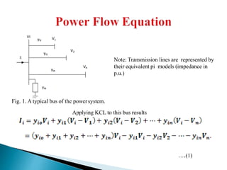
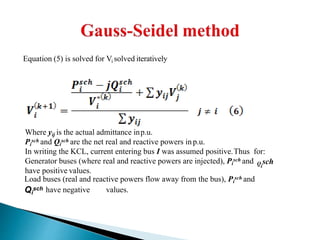
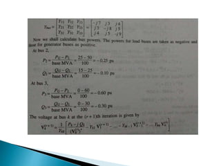
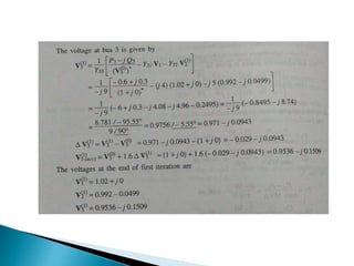
This document discusses load flow analysis using the Gauss-Seidel iterative method. Load flow studies calculate voltage drops, bus voltages, and power flows under normal and contingency conditions to ensure system voltages and equipment loads remain within limits. They are used to identify need for additional generation or reactive support. The Gauss-Seidel method models the power system buses and solves the nonlinear load flow equations iteratively to determine voltages and power flows throughout the system. It provides an example three bus system to demonstrate forming the bus admittance matrix and performing the first iteration to solve for voltages at two buses.

1. Subject:- Interconnected Power System
Topic:- Gauss Seidel Methode
Prepared By :
Yash kothadia (150110109019)
Abhishek lalkiya (150110109020)
keyur nimavat (150110109027)

3.  Load-flow studies are performed to determine the steady-state
operation of an electric power system. It calculates the voltage
drop on each feeder, the voltage at each bus, and the power
flow in all branch and feeder circuits.
 Determine if system voltages remain within specified limits
under various contingency conditions, and whether equipment
such as transformers and conductors are overloaded.
 Load-flow studies are often used to identify the need for
additional generation, capacitive, or inductive VAR support, or
the placement of capacitors and/or reactors to maintain system
voltages within specified limits.
 Losses in each branch and total system power losses are also
calculated.
 Necessary for planning, economic scheduling, and control of an
existing system as well as planning its future expansion of
system.

4. Note: Transmission lines are represented by
their equivalent pi models (impedance in
p.u.)
Fig. 1. A typical bus of the powersystem.
Applying KCL to this bus results
….(1)

5. ….(2)
The real and reactive power at bus
i is
Substituting for Ii in (2) yields
Equation (5) is an algebraic non linear equation which must be
solved by iterative techniques

6. Equation (5) is solved for Vi solved iteratively
Where yij is the actual admittance inp.u.
Pi
sch and Qi
sch are the net real and reactive powers inp.u.
In writing the KCL, current entering bus I was assumed positive.Thus for:
Generator buses (where real and reactive powers are injected), Pi
sch and
have positive values.
Qi
sch
Load buses (real and reactive powers flow away from the bus), Pi
sch and
Qi
sch have negative values.

7. Eqn.5 can be solved for Pi andQi
The power flow equation is usually expressed in terms of the elements of the bus
admittance matrix, Ybus , shown by upper case letters, are Yij = -yij, and the diagonal
elements are Yii = ∑ yij. Hence eqn. 6 can be written as

8. Iterative steps:
•Slack bus: both components of the voltage are specified. 2(n-1)
equations to be solved iteratively.
• Flat voltage start: initial voltage of 1.0+j0 for unknown voltages.
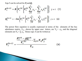
• PQ buses: Pi and Qi are known. with flat voltage start, Eqn. 9 is solved
for real and imaginary components of Voltage.
i•PV buses: Psch and i[Vi] are known. Eqn. 11 is solved for Q k+1 which is
then substituted in Eqn. 9 to solve for Vi
k+1

9.  A three bus system are shown in figure. The relevent per unit values of
admittences on 100 MVA base are indicated on the diagram and bus data
are given in table-
Form Ybus and determine the voltage at bus 2 and bus bus 3 after the first
iteration using Gauss- Siedel method.Take the acceleration factor 1.6.
(Power System Analysis by Ashfaq Hussain,page no. 380)

11.  We first calculate the element of the Ybus
 Y11 =sum of admittences of all elements connected to node 1=-j3-j4=-
j7
• Y22 =sum of all admittances connected to
bus 2=-
j3-j4=-j8
• Y33=sum of all the admittances connected
to bus 3=-j4-j5=-j9
• Y12=Y21=-(-j3)=j3
•Y23=Y32=-(j5)=j5
•Y31=Y13=-(-j4)=j4