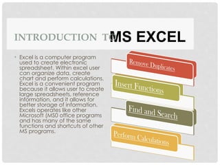
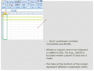
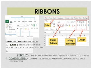
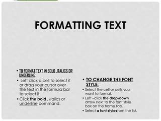
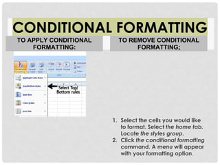
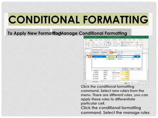
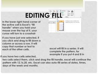
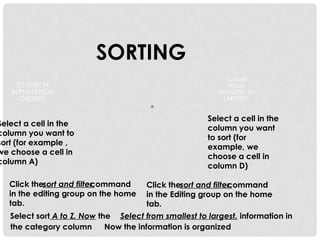
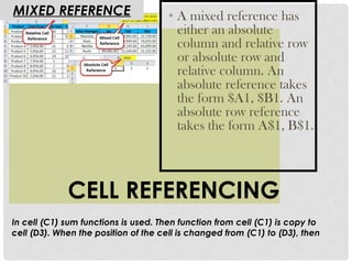
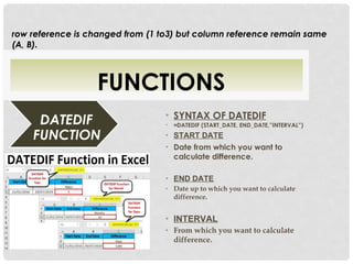
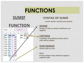
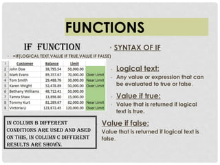
EXCEL
MS
PRESENTATION ON
NRO0502781
VATSA
TARKIK
BY:
MS programs.
functions and shortcuts of other
and has many of the same
Microsoft (MS0 office programs
Excels operates like other
better storage of information.
information, and it allows for
large spreadsheets, reference
because it allows user to create
Excel is a convenient program
chart and perform calculations.
can organize data, create
spreadsheet. Within excel user
used to create electronic
Excel is a computer program
•
MS EXCEL
INTRODUCTION TO
OVERVIEW OF EXCEL
 Microsoft excel consists of workbooks.
Within each workbook, there is an
infinite number of worksheets.
  Each worksheet contains
COLUMNS and ROWS.
 Where a column and a row intersect
is called a CELL. For e.g., cell D5 is
located where column D and row 5
meet.
 The tabs at the bottom of the screen
represent different worksheets within
a workbook. You can use the
scrolling buttons on the left to bring
other worksheets into view.
OFFICE BUTTON
(CTRL+W)
TO CLOSE A DOCUMENT
–
CLOSE
TO DISTRIBUTE DOCUMENT TO OTHER PEOPLE
-
PUBLISH
TO SEND A COPY OF DOCUMENT TO OTHER PEOPLE
-
SEND
TO PREPARE DOCUMENT FOR DITRIBUTION
–
PREPARE
)
CTRL+P
(
TO PRINT A DOCUMENT
–
PRINT
(F12)
TO SAVE COPY DOCUMENT
-
SAVE AS
CTRL+S)
(
TO SAVE A DOCUMENT
-
SAVE
)
CTRL+O
(
TO OPEN EXISTING DOCUMENT
-
–
OPEN
)
CTRL+N
(
TO OPEN NEW WORKBOOK
-
-
NEW
RIBBONS
GROUPS: GROUPS ARE SETS OF RELATED COMMANDS, DISPLAYED ON TABS.
3. COMMANDS: A COMMAND IS A BUTTON, AMENU OR A BOX WHERE YOU ENER
INFORMATION.
2.
.
ACROSS THE TOP OF THE EXCEL WINDOW
THERE ARE SEVEN TABS
:
TABS
1.
THREE PARTS OF THE RIBBON ARE
•
TO COPY AND PASTE CONTENTS: Select the
cell or cells you wish to copy. Click the copy
command in the clipboard group on the home
tab.
Select the cell or cells where you want to paste the
information.
WORKING WITH CELLS
Click the paste command and the copied information
now appear in the new cells.
WORKING WITH CELLS
removed and now appear in the new cells.
The command information will be

paste command.
Click the

.
paste the information
Select the cell or cells where you want to

group on the home tab.
in the clipboard
the cut commands
Click

Select the cell or cell you wish to cut.

CONTENTS:
TO CUT AND PASTE CELL
FORMATTING TEXT
from the list.
a font styles
Select
•
box on the home tab.
arrow next to the font style
down
-
the drop
click
–
Left
•
want to format.
Select the cell or cells you
•
STYLE:
TO CHANGE THE FONT
•
command.
underline
or
, italics
the bold
Click
•
to select it.
the text in the formula bar
or drag your cursor over
Left click a cell to select it
•
:
UNDERLINE
TO FORMAT TEXT IN BOLD ,ITALICS OR
•
FORMATTING TEXT
To Change the Text Colour To Add a Fill Colour
Select the cells or cells you want
to format.
Left click the drop-down arrow
next to the text colour command.
A colour palette will be appearing
and select the colour from the
palette.
Select the cell or cells you want
to format.
Click the fill command. A colour
palette will be appearing.
Select a colour from the palette.
1. Select the cells you would like
to format. Select the home tab.
Locate the styles group.
2. Click the conditional formatting
command. A menu will appear
with your formatting option.
CONDITIONAL FORMATTING
TO APPLY CONDITIONAL
FORMATTING:
TO REMOVE CONDITIONAL
FORMATTING:
1. Click the conditional Formatting
command. Select the clear
rules.
2. Choose to clear rules from the
entire worksheet or the selected
cells.
Click the conditional formatting
command. Select new rulers from the
menu. There are different rules, you can
apply these rules to differentiate
particular cell.
Click the conditional formatting
command. Select the manage rules
CONDITIONAL FORMATTING
To Apply New Formatting
To Manage Conditional Formatting
from the menu. The conditional
formatting rules manager dialog
box will be appearing. From here
you can edit a rule, delete a rule or
change the order of rules.
TO INSERT ROWS AND COLUMNS
Note:
appear.
the home tab. The column will
command in the cells group on
appear. Click the insert
where you want the column to
Select the column to the right of
TO INSERT COLUMNS
.
tab. The row will appear
on the home
group
command in the cells
appear. Click the insert
to
new row
Select the row below where you want the
TO INSERT
1. The new row always appears above the selected row.
2. The new column always appears to the left of the selected column.
If you have two cells selected,
two cells select them, click and drag the fill handle, excel will continue the
pattern with 12,16,20, etc. Excel can also auto-fill series of dates, times,
days of the week and months.
EDITING FILL
example if you put 4 and 8 in
complete the pattern, for
excel will fill in a series. It will
each of the other cells.
copy that number or text to
column or across a row, it will
you click and drag to fill down a
If you have just one selected, if
.
cursor will turn to a crosshair
mouse over the top of it, your
handle” when you hold your
the active cell is Excel’s “fill
In the lower right-hand corner of
Select sort A to Z. Now the Select from smallest to largest. information in
the category column Now the information is organized
SORTING
tab.
in the Editing group on the home
command
sort and filter
Click the
column D)
choose a cell in
example, we
to sort (for
column you want
Select a cell in the
LARGEST:
SMALLEST TO
FROM
TO SORT
tab.
in the editing group on the home
command
sort and filter
Click the
column A)
we choose a cell in
sort (for example ,
column you want to
Select a cell in the
ORDERS:
ALPHABETICAL
TO SORT IN
•
is organized in alphabetical from the smallest to largest orders. amount.
CELL REFERENCING
To (A5, B5).
reference is also changed from (A4, B4)
changed from (E4) to (F5), then the
F5). When position of the cell is
(
Then function from (E4) is copy to cell
In cell (E4) sum function is used.
changed.
changes, the reference itself is
contains the reference
the position of the cell that
relative position of the cell. If
as based (A1) is based on the
A RELATIVE CELL REFERENCE
CELL REFERENCING
ABSOLUTE CELL REFERENCING
• An Absolute cell reference as
($A$1) always refers to a cell
in a cell in a specific location.
If the position of the cell that
contains the formula
changes, absolute reference
remains the same.
• In cell (C1) sum functions is
used. Then function from cell
(C1) is copy to cell (D3).
When the positions of the cell
is changed from (C1) to (D3) ,
then the absolute reference
remains the same (A1,B1). $
is used for constant row or
column.
CELL REFERENCING
In cell (C1) sum functions is used. Then function from cell (C1) is copy to
cell (D3). When the position of the cell is changed from (C1) to (D3), then
MIXED REFERENCE • A mixed reference has
either an absolute
column and relative row
or absolute row and
relative column. An
absolute reference takes
the form $A1, $B1. An
absolute row reference
takes the form A$1, B$1.
row reference is changed from (1 to3) but column reference remain same
(A, B).
FUNCTIONS
FUNCTION
DATEDIF
difference.
From which you want to calculate
•
INTERVAL
•
difference.
Date up to which you want to calculate
•
END DATE
•
calculate difference.
Date from which you want to
•
START DATE
•
DATEDIF (START_DATE, END_DATE,”INTERVAL”)
=
•
SYNTAX OF DATEDIF
•
FUNCTIONS
SUMIF • SYNTAX OF SUMIF
• =SUMIF (RANGE, CRITERIA,SUM_RANGE)
FUNCTION
used for sum
If sum range is not used tan range is
•
Note:
•
Actual cells to sum.
•
SUM RANGES
•
cells will be added.
Condition that defines which cell or
•
CRITERIA
•
applied.
Range of cells on which conditions are
•
RANGE
•
FUNCTIONS
IF FUNCTION • SYNTAX OF IF
• =IF(LOGICAL TEXT,VALUE IF TRUE,VALUE IF FALSE)
• Logical text:
• Any value or expression that can
be evaluated to true or false.
• Value if true:
• Value that is returned if logical
text is true.
• Value if false:
• Value that is returned if logical text is
false.
IN COLUMN B DIFFERENT
CONDITIONS ARE USED AND ASED
ON THIS, IN COLUMN C DIFFERENT
RESULTS ARE shown.
FUNCTIONS
COUNT FUNCTIONS
Count only cells that contains number.
Count cells that are not empty.
Count cells that are blank. Count number of
cells that meet given condition.
• Syntax of functions
• 1. COUNT
• =COUNT (VALUE1, VALUE2……)
• 2. COUNTA
• =COUNTA (VALUE1,VALUE2….)
• 3. COUNTBLANK
• =COUNTBLANK(RANGE)
• 4 COUNTIF
• =COUNTIF (RANGE, CRITERIA)
TEXT FUNCTIONS
• SYNTAX OF FUNCTION
• LOWER FUNCTION
• =LOWER(TEXT)
• UPPER FUNCTION
• =UPPER(TEXT)
• PROPER FUNCTION
1. To convert text from capital to •
=PROPER(TEXT) small.
2. To convert text from small to
capital.
3. To capitalized each word of text.
TEXT FUNCTIONS
• SYNTAX OF FUNCTIONS
• 1. LEFT FUNCTIONS
• =LEFT (TEXT, NUM_CHARS)
• 2. RIGHT FUNCTION
• =RIGHT (TEXT, NUM_CHARS)
1. Return specified no. of character from start
of text.
2. Return specified no. of character from end
of text.
3. Return character from middle of text, given
a starting position.
• 3. MID FUNCTION
• =MID (TEXT, STARTNUM, NUM_CH ARS)
OTHER FUNCTIONS
.
STRING
CHARACTERS IN A TEXT
RETURN THE NO. OF
LEN
DIVIDED BY A DIVISOR.
REMAINDER AFTER A NO. IS
RETURNS THE
MOD
DATE ONLY
RETURNS CURRENT
TODAY
DATE AND TIME.
RETURNS CURRENT
NOW
:
USES OF FUNCTIONS
FUNCTION AUDITING
• TRACE PRECEDENTS
• Show arrow that indicate what cells
affect the value of the currently
selected cell.
• For example, cell A1 and A3 affect
the value of cell C6.
• TRACE DEPENDENTS
• Show arrow that indicate what cells
are affected by the value of the
currently selected cell.
• In this example cell C2 and C6 are
affected by the value of cell A2
and cell C6 is also affected by the
cell A4.
PowerPoint presentation on Microsoft Excel.docx

PowerPoint presentation on Microsoft Excel.docx

  • 1.
  • 2.
    MS programs. functions andshortcuts of other and has many of the same Microsoft (MS0 office programs Excels operates like other better storage of information. information, and it allows for large spreadsheets, reference because it allows user to create Excel is a convenient program chart and perform calculations. can organize data, create spreadsheet. Within excel user used to create electronic Excel is a computer program • MS EXCEL INTRODUCTION TO
  • 3.
    OVERVIEW OF EXCEL Microsoft excel consists of workbooks. Within each workbook, there is an infinite number of worksheets.
  • 4.
      Eachworksheet contains COLUMNS and ROWS.  Where a column and a row intersect is called a CELL. For e.g., cell D5 is located where column D and row 5 meet.  The tabs at the bottom of the screen represent different worksheets within
  • 5.
    a workbook. Youcan use the scrolling buttons on the left to bring other worksheets into view.
  • 6.
    OFFICE BUTTON (CTRL+W) TO CLOSEA DOCUMENT – CLOSE TO DISTRIBUTE DOCUMENT TO OTHER PEOPLE - PUBLISH TO SEND A COPY OF DOCUMENT TO OTHER PEOPLE - SEND TO PREPARE DOCUMENT FOR DITRIBUTION – PREPARE ) CTRL+P ( TO PRINT A DOCUMENT – PRINT (F12) TO SAVE COPY DOCUMENT - SAVE AS CTRL+S) ( TO SAVE A DOCUMENT - SAVE ) CTRL+O ( TO OPEN EXISTING DOCUMENT - – OPEN ) CTRL+N ( TO OPEN NEW WORKBOOK - - NEW
  • 7.
    RIBBONS GROUPS: GROUPS ARESETS OF RELATED COMMANDS, DISPLAYED ON TABS. 3. COMMANDS: A COMMAND IS A BUTTON, AMENU OR A BOX WHERE YOU ENER INFORMATION. 2. . ACROSS THE TOP OF THE EXCEL WINDOW THERE ARE SEVEN TABS : TABS 1. THREE PARTS OF THE RIBBON ARE •
  • 8.
    TO COPY ANDPASTE CONTENTS: Select the cell or cells you wish to copy. Click the copy command in the clipboard group on the home tab. Select the cell or cells where you want to paste the information. WORKING WITH CELLS
  • 9.
    Click the pastecommand and the copied information now appear in the new cells.
  • 10.
    WORKING WITH CELLS removedand now appear in the new cells. The command information will be  paste command. Click the  . paste the information Select the cell or cells where you want to  group on the home tab. in the clipboard the cut commands Click  Select the cell or cell you wish to cut.  CONTENTS: TO CUT AND PASTE CELL
  • 11.
    FORMATTING TEXT from thelist. a font styles Select • box on the home tab. arrow next to the font style down - the drop click – Left • want to format. Select the cell or cells you • STYLE: TO CHANGE THE FONT • command. underline or , italics the bold Click • to select it. the text in the formula bar or drag your cursor over Left click a cell to select it • : UNDERLINE TO FORMAT TEXT IN BOLD ,ITALICS OR •
  • 12.
    FORMATTING TEXT To Changethe Text Colour To Add a Fill Colour Select the cells or cells you want to format. Left click the drop-down arrow next to the text colour command. A colour palette will be appearing and select the colour from the palette. Select the cell or cells you want to format. Click the fill command. A colour palette will be appearing. Select a colour from the palette.
  • 13.
    1. Select thecells you would like to format. Select the home tab. Locate the styles group. 2. Click the conditional formatting command. A menu will appear with your formatting option. CONDITIONAL FORMATTING TO APPLY CONDITIONAL FORMATTING: TO REMOVE CONDITIONAL FORMATTING:
  • 14.
    1. Click theconditional Formatting command. Select the clear rules. 2. Choose to clear rules from the entire worksheet or the selected cells.
  • 15.
    Click the conditionalformatting command. Select new rulers from the menu. There are different rules, you can apply these rules to differentiate particular cell. Click the conditional formatting command. Select the manage rules CONDITIONAL FORMATTING To Apply New Formatting To Manage Conditional Formatting
  • 16.
    from the menu.The conditional formatting rules manager dialog box will be appearing. From here you can edit a rule, delete a rule or change the order of rules.
  • 17.
    TO INSERT ROWSAND COLUMNS Note: appear. the home tab. The column will command in the cells group on appear. Click the insert where you want the column to Select the column to the right of TO INSERT COLUMNS . tab. The row will appear on the home group command in the cells appear. Click the insert to new row Select the row below where you want the TO INSERT
  • 18.
    1. The newrow always appears above the selected row. 2. The new column always appears to the left of the selected column.
  • 20.
    If you havetwo cells selected, two cells select them, click and drag the fill handle, excel will continue the pattern with 12,16,20, etc. Excel can also auto-fill series of dates, times, days of the week and months. EDITING FILL example if you put 4 and 8 in complete the pattern, for excel will fill in a series. It will each of the other cells. copy that number or text to column or across a row, it will you click and drag to fill down a If you have just one selected, if . cursor will turn to a crosshair mouse over the top of it, your handle” when you hold your the active cell is Excel’s “fill In the lower right-hand corner of
  • 21.
    Select sort Ato Z. Now the Select from smallest to largest. information in the category column Now the information is organized SORTING tab. in the Editing group on the home command sort and filter Click the column D) choose a cell in example, we to sort (for column you want Select a cell in the LARGEST: SMALLEST TO FROM TO SORT tab. in the editing group on the home command sort and filter Click the column A) we choose a cell in sort (for example , column you want to Select a cell in the ORDERS: ALPHABETICAL TO SORT IN •
  • 22.
    is organized inalphabetical from the smallest to largest orders. amount. CELL REFERENCING To (A5, B5). reference is also changed from (A4, B4) changed from (E4) to (F5), then the F5). When position of the cell is ( Then function from (E4) is copy to cell In cell (E4) sum function is used. changed. changes, the reference itself is contains the reference the position of the cell that relative position of the cell. If as based (A1) is based on the A RELATIVE CELL REFERENCE
  • 23.
    CELL REFERENCING ABSOLUTE CELLREFERENCING • An Absolute cell reference as ($A$1) always refers to a cell in a cell in a specific location. If the position of the cell that contains the formula changes, absolute reference remains the same. • In cell (C1) sum functions is used. Then function from cell (C1) is copy to cell (D3). When the positions of the cell is changed from (C1) to (D3) , then the absolute reference remains the same (A1,B1). $ is used for constant row or column.
  • 24.
    CELL REFERENCING In cell(C1) sum functions is used. Then function from cell (C1) is copy to cell (D3). When the position of the cell is changed from (C1) to (D3), then MIXED REFERENCE • A mixed reference has either an absolute column and relative row or absolute row and relative column. An absolute reference takes the form $A1, $B1. An absolute row reference takes the form A$1, B$1.
  • 25.
    row reference ischanged from (1 to3) but column reference remain same (A, B). FUNCTIONS FUNCTION DATEDIF difference. From which you want to calculate • INTERVAL • difference. Date up to which you want to calculate • END DATE • calculate difference. Date from which you want to • START DATE • DATEDIF (START_DATE, END_DATE,”INTERVAL”) = • SYNTAX OF DATEDIF •
  • 26.
    FUNCTIONS SUMIF • SYNTAXOF SUMIF • =SUMIF (RANGE, CRITERIA,SUM_RANGE) FUNCTION used for sum If sum range is not used tan range is • Note: • Actual cells to sum. • SUM RANGES • cells will be added. Condition that defines which cell or • CRITERIA • applied. Range of cells on which conditions are • RANGE •
  • 27.
    FUNCTIONS IF FUNCTION •SYNTAX OF IF • =IF(LOGICAL TEXT,VALUE IF TRUE,VALUE IF FALSE) • Logical text: • Any value or expression that can be evaluated to true or false. • Value if true: • Value that is returned if logical text is true. • Value if false: • Value that is returned if logical text is false. IN COLUMN B DIFFERENT CONDITIONS ARE USED AND ASED ON THIS, IN COLUMN C DIFFERENT RESULTS ARE shown.
  • 28.
    FUNCTIONS COUNT FUNCTIONS Count onlycells that contains number. Count cells that are not empty. Count cells that are blank. Count number of cells that meet given condition. • Syntax of functions • 1. COUNT • =COUNT (VALUE1, VALUE2……) • 2. COUNTA • =COUNTA (VALUE1,VALUE2….) • 3. COUNTBLANK • =COUNTBLANK(RANGE) • 4 COUNTIF
  • 29.
    • =COUNTIF (RANGE,CRITERIA) TEXT FUNCTIONS • SYNTAX OF FUNCTION • LOWER FUNCTION • =LOWER(TEXT) • UPPER FUNCTION • =UPPER(TEXT) • PROPER FUNCTION 1. To convert text from capital to • =PROPER(TEXT) small. 2. To convert text from small to capital.
  • 30.
    3. To capitalizedeach word of text. TEXT FUNCTIONS • SYNTAX OF FUNCTIONS • 1. LEFT FUNCTIONS • =LEFT (TEXT, NUM_CHARS) • 2. RIGHT FUNCTION • =RIGHT (TEXT, NUM_CHARS) 1. Return specified no. of character from start of text. 2. Return specified no. of character from end of text. 3. Return character from middle of text, given a starting position.
  • 31.
    • 3. MIDFUNCTION • =MID (TEXT, STARTNUM, NUM_CH ARS)
  • 32.
    OTHER FUNCTIONS . STRING CHARACTERS INA TEXT RETURN THE NO. OF LEN DIVIDED BY A DIVISOR. REMAINDER AFTER A NO. IS RETURNS THE MOD DATE ONLY RETURNS CURRENT TODAY DATE AND TIME. RETURNS CURRENT NOW : USES OF FUNCTIONS
  • 33.
    FUNCTION AUDITING • TRACEPRECEDENTS • Show arrow that indicate what cells affect the value of the currently selected cell.
  • 34.
    • For example,cell A1 and A3 affect the value of cell C6. • TRACE DEPENDENTS • Show arrow that indicate what cells are affected by the value of the currently selected cell. • In this example cell C2 and C6 are affected by the value of cell A2 and cell C6 is also affected by the cell A4.