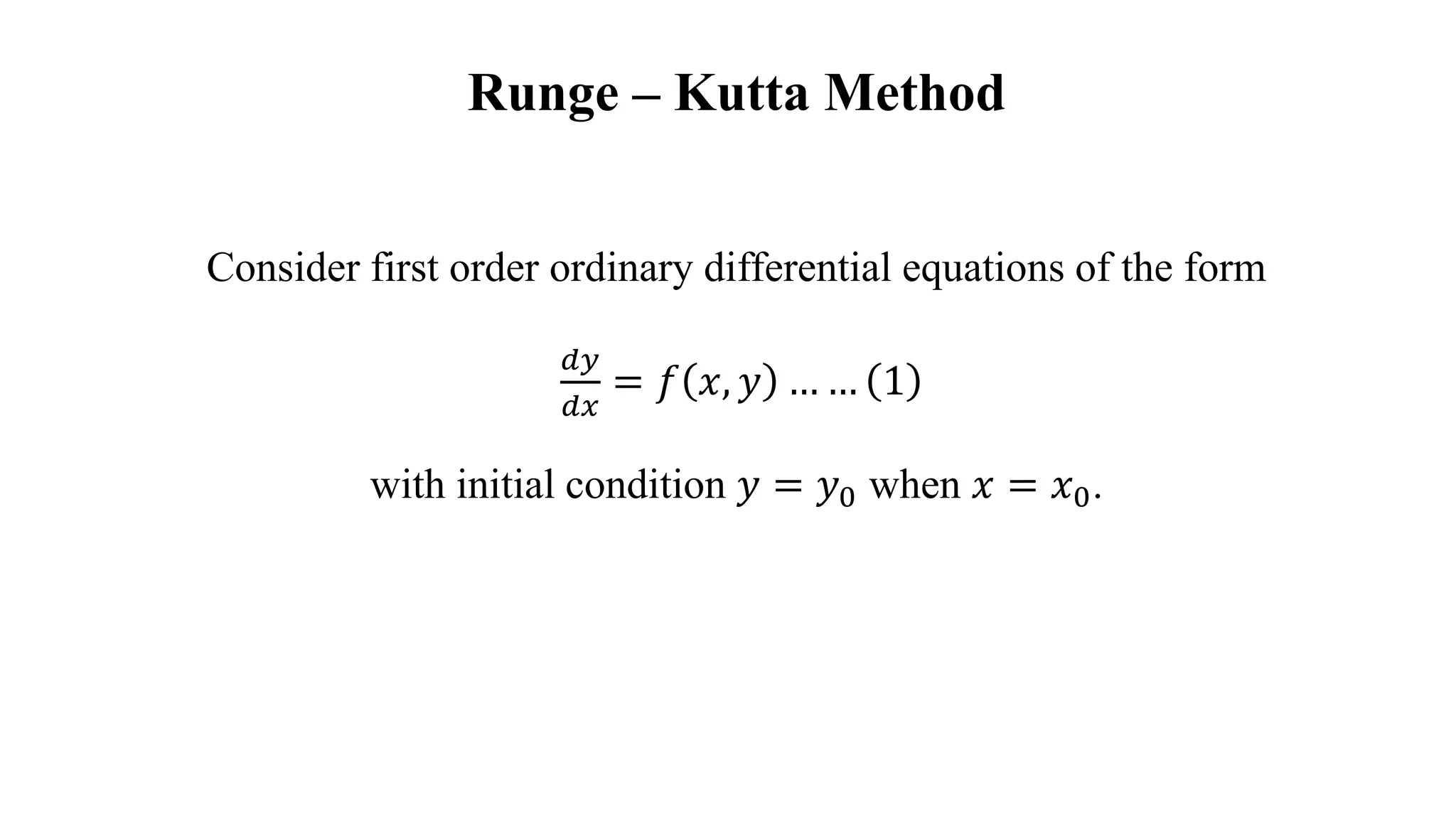
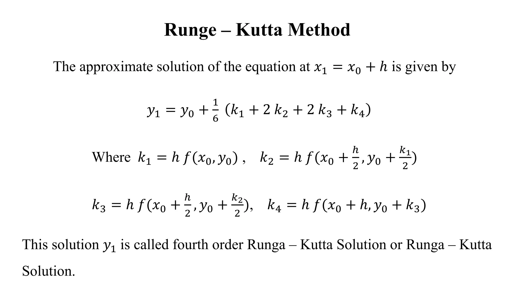
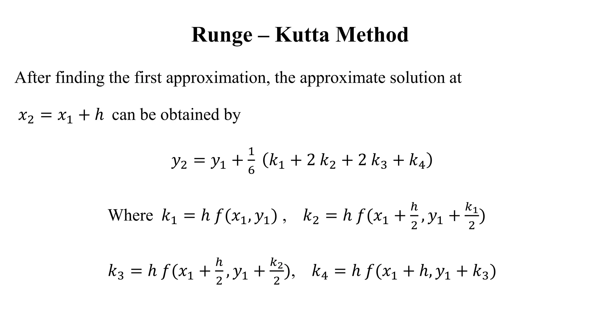
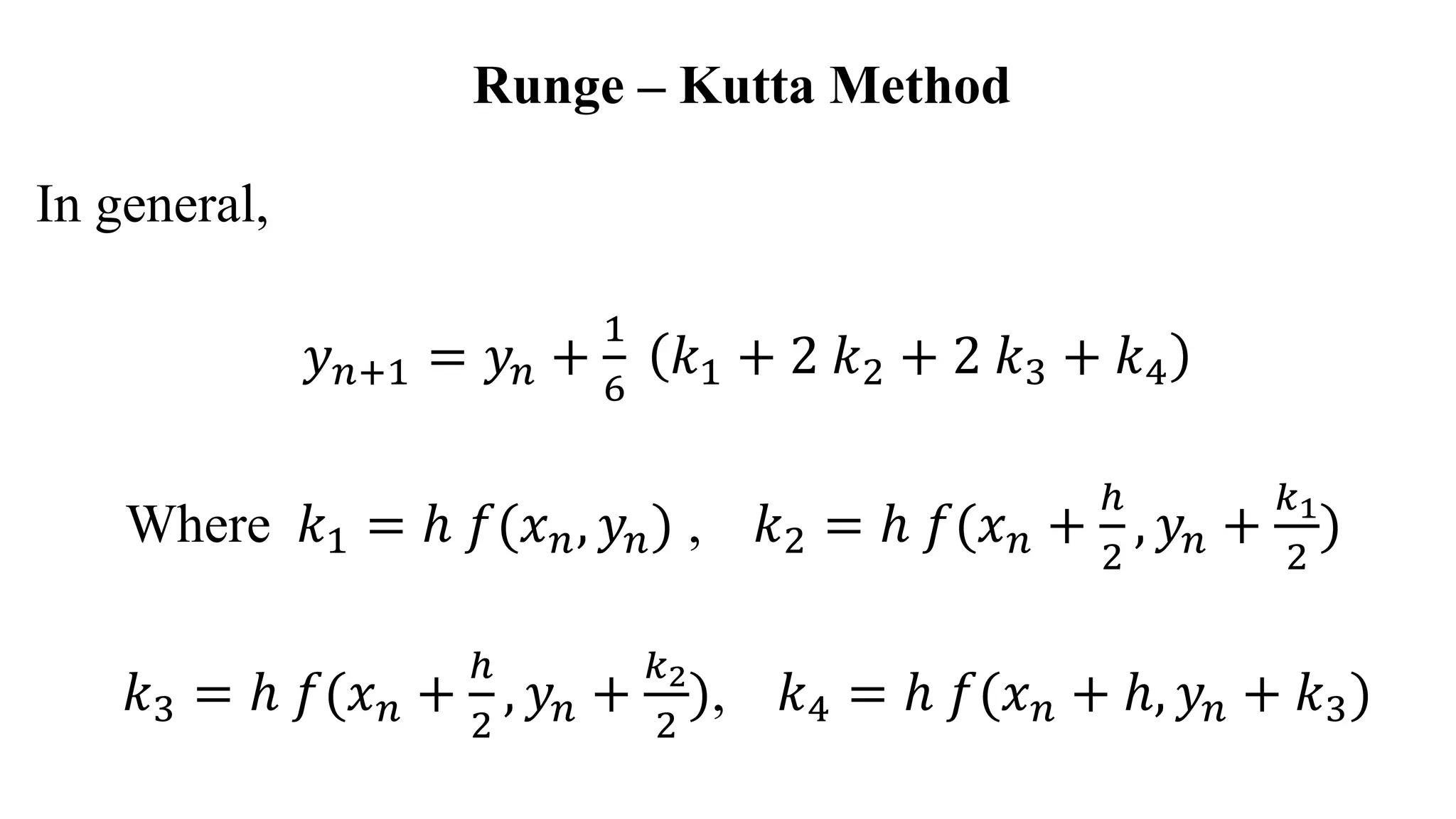
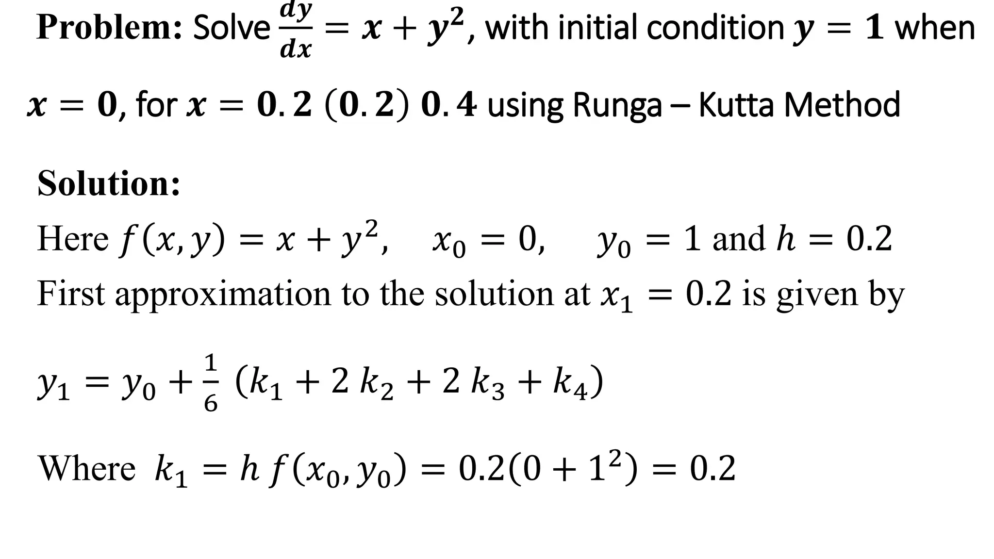
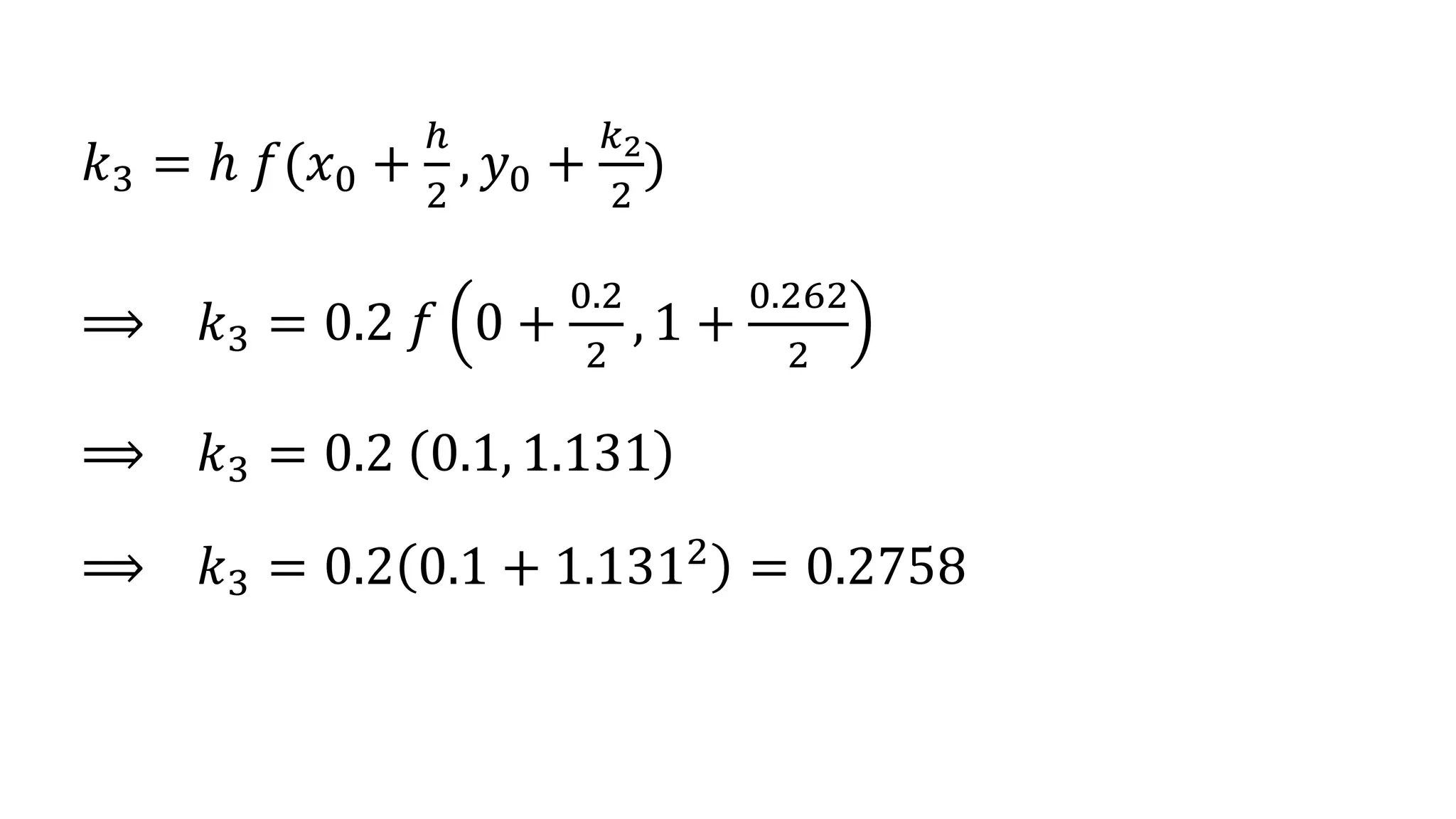
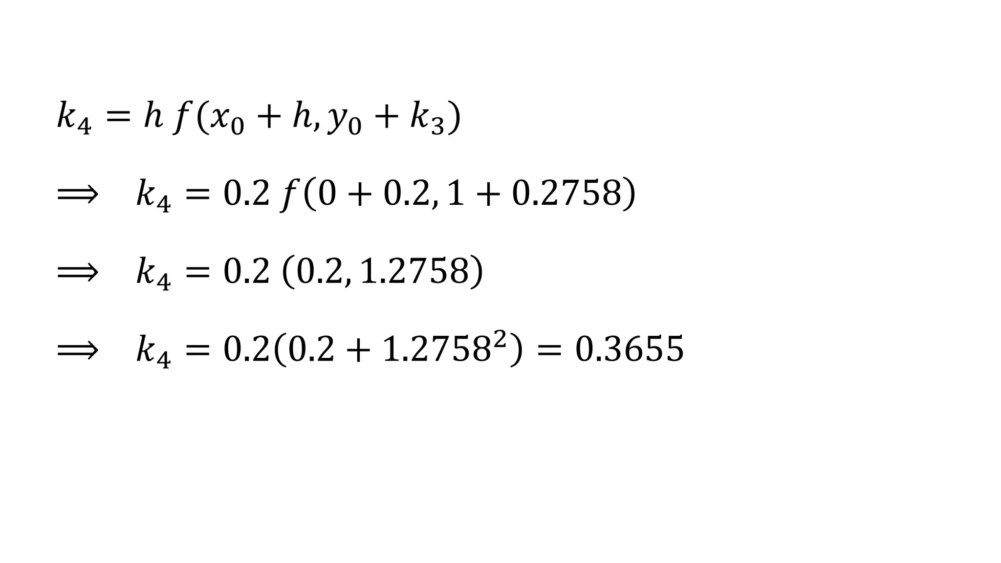
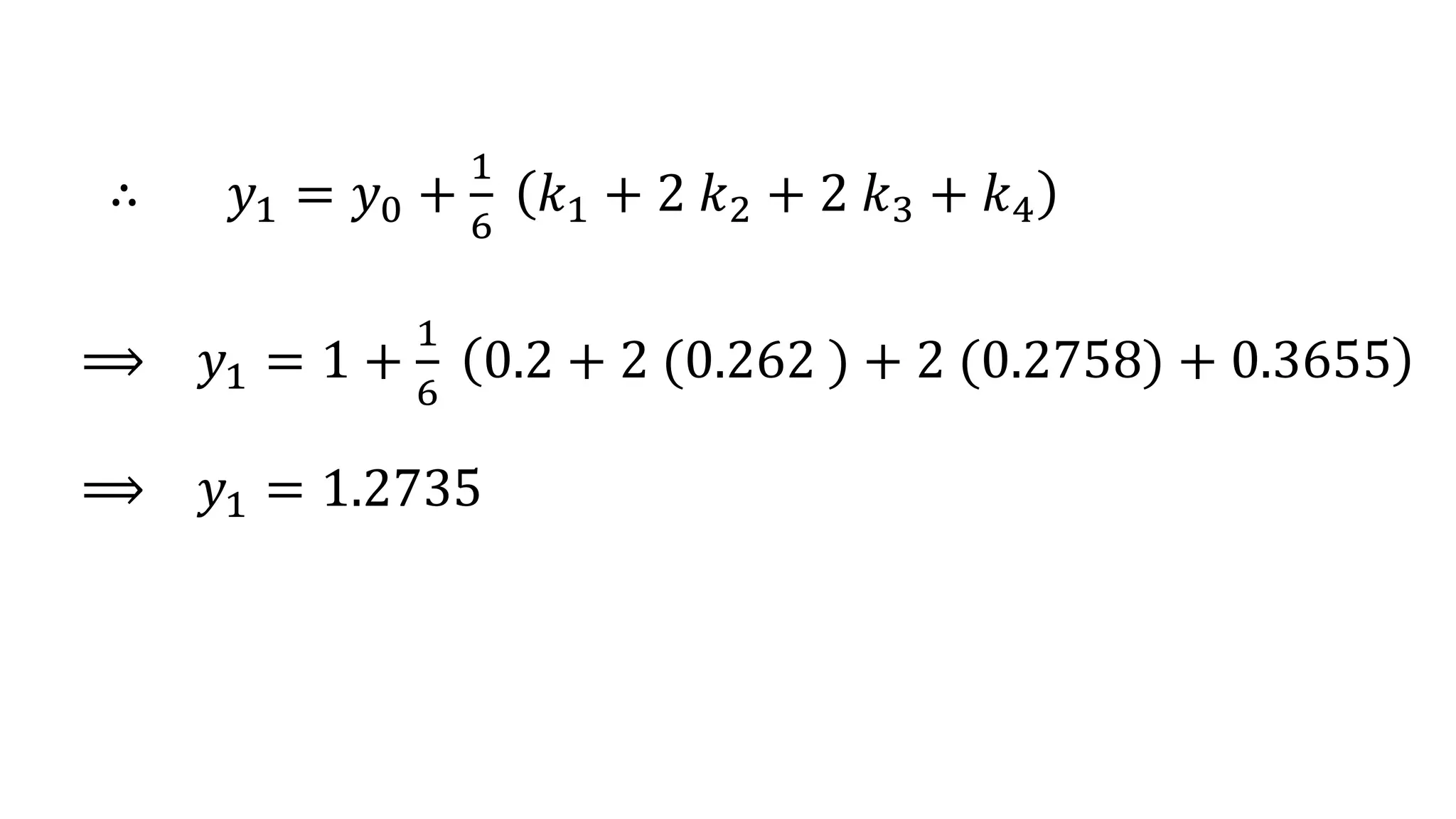
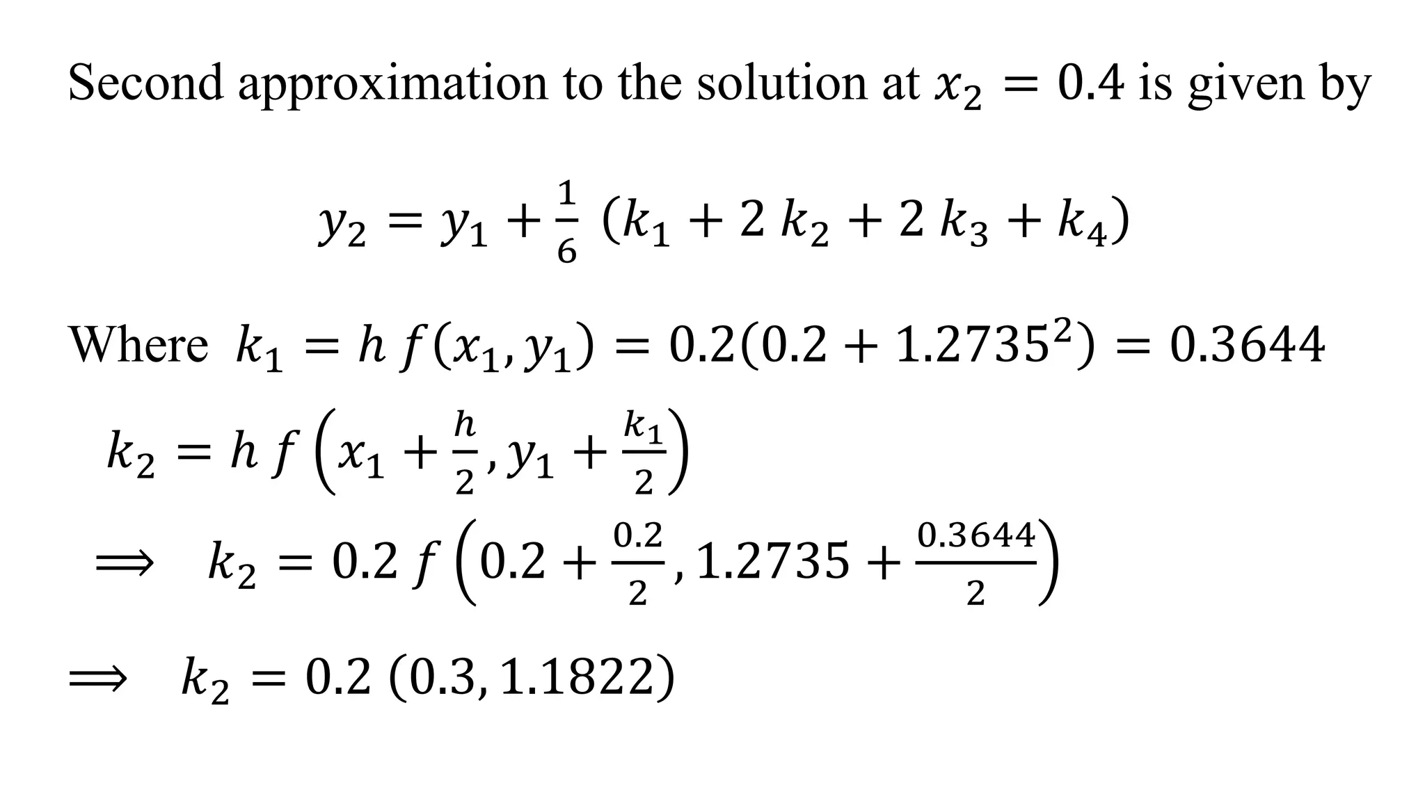
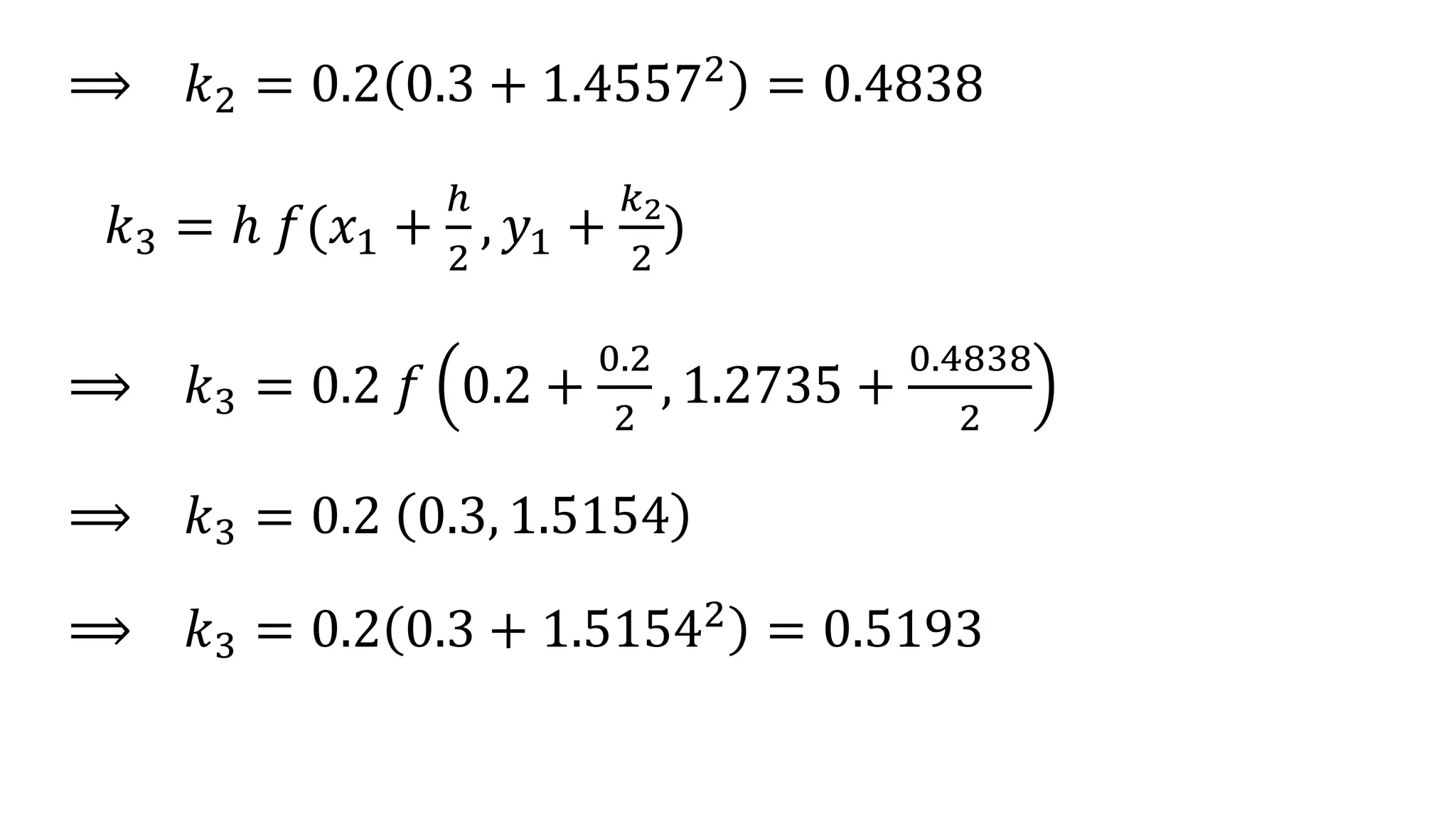
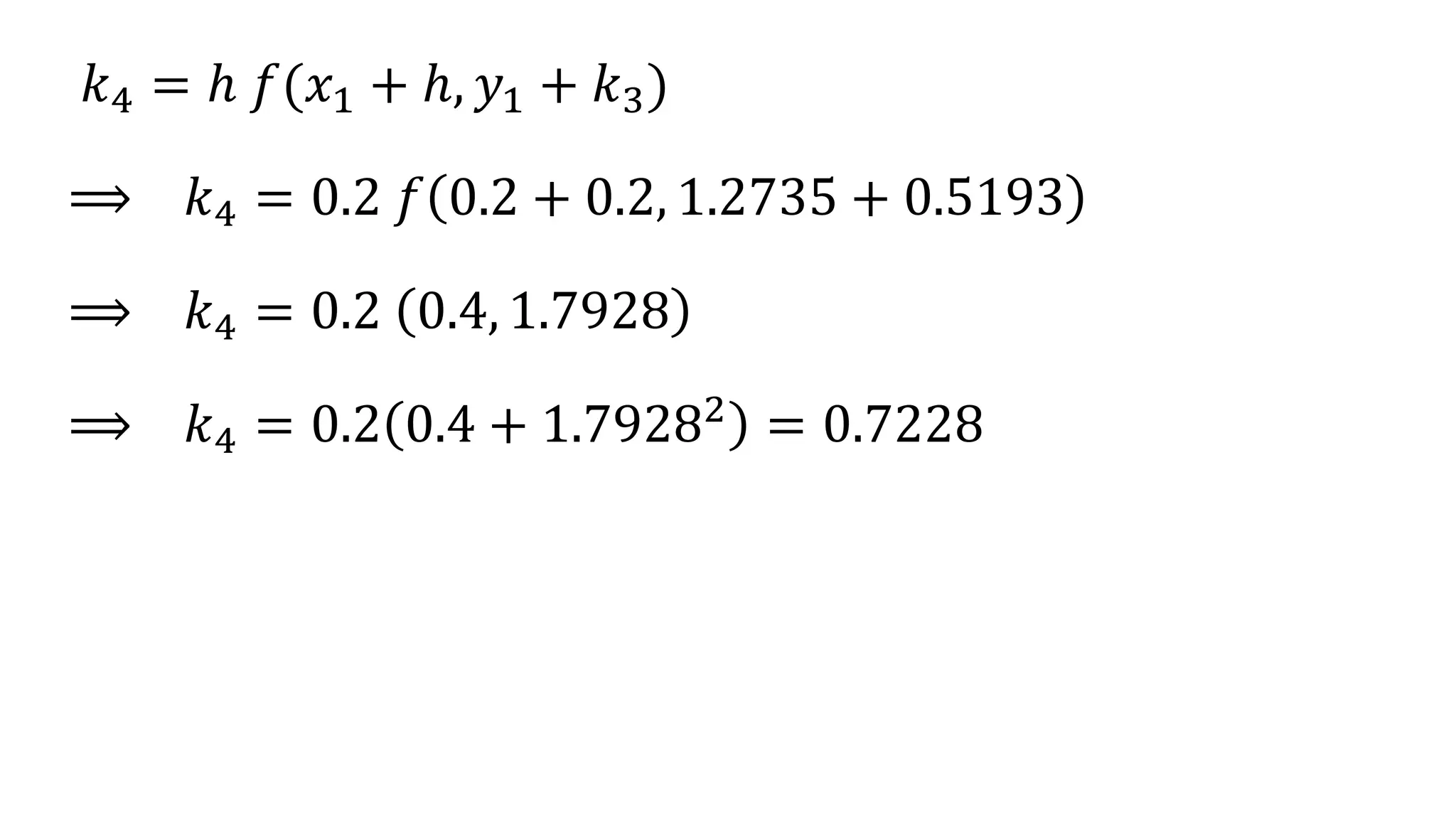
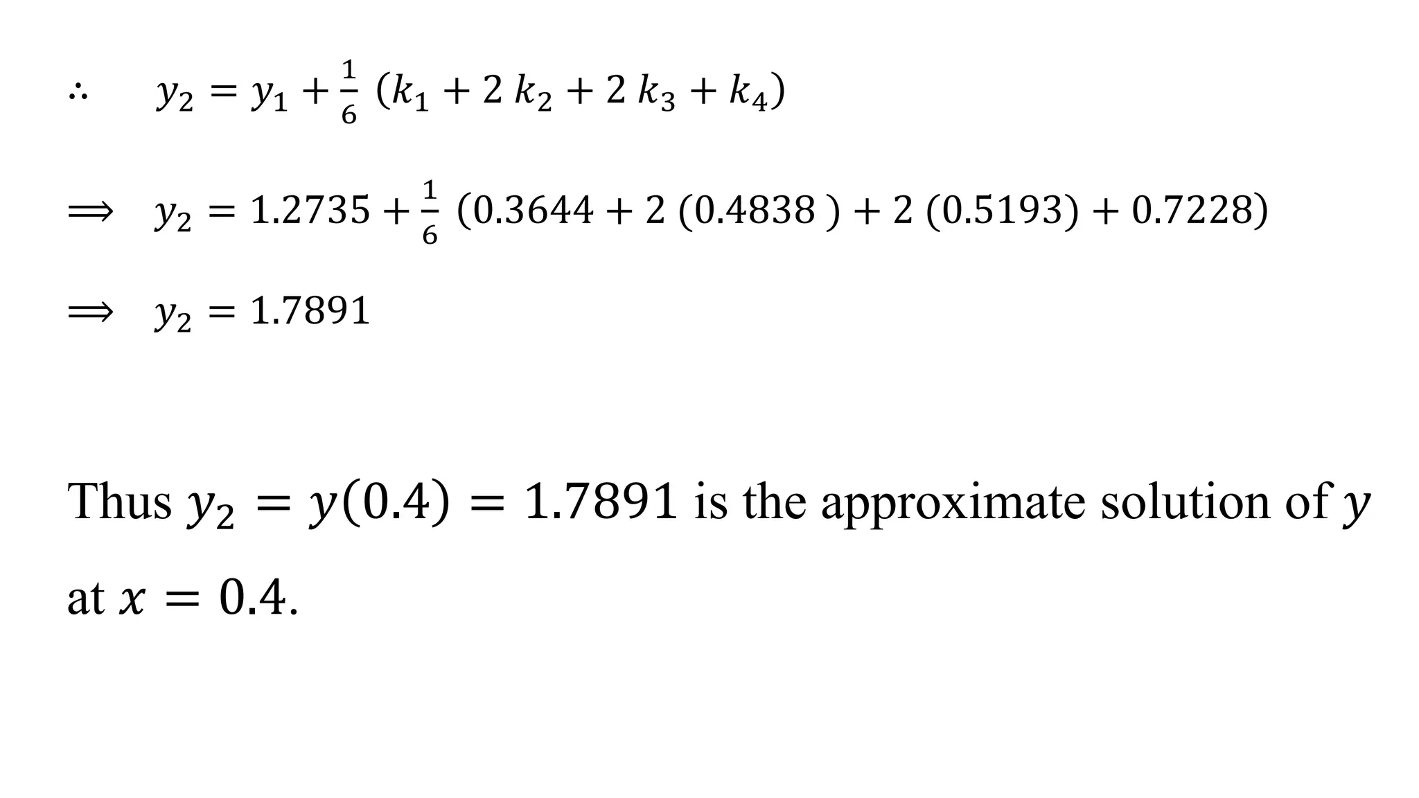
Runge – Kutta Method of 4th Order
21UMT2T462: Numerical Analysis
Dr. Soya Mathew
Assistant Professor in Mathematics
Department of Physical Sciences
Kristu Jayanti College (Autonomous)
Bengaluru – 560077, India
Runge – Kutta Method
Consider first order ordinary differential equations of the form
𝑑𝑦
𝑑𝑥
= 𝑓 𝑥, 𝑦 … … 1
with initial condition 𝑦 = 𝑦0 when 𝑥 = 𝑥0.
Runge – Kutta Method
The approximate solution of the equation at 𝑥1 = 𝑥0 + ℎ is given by
𝑦1 = 𝑦0 +
1
6
𝑘1 + 2 𝑘2 + 2 𝑘3 + 𝑘4
Where 𝑘1 = ℎ 𝑓(𝑥0, 𝑦0) , 𝑘2 = ℎ 𝑓(𝑥0 +
ℎ
2
, 𝑦0 +
𝑘1
2
)
𝑘3 = ℎ 𝑓(𝑥0 +
ℎ
2
, 𝑦0 +
𝑘2
2
), 𝑘4 = ℎ 𝑓(𝑥0 + ℎ, 𝑦0 + 𝑘3)
This solution 𝑦1 is called fourth order Runga – Kutta Solution or Runga – Kutta
Solution.
Runge – Kutta Method
After finding the first approximation, the approximate solution at
𝑥2 = 𝑥1 + ℎ can be obtained by
𝑦2 = 𝑦1 +
1
6
𝑘1 + 2 𝑘2 + 2 𝑘3 + 𝑘4
Where 𝑘1 = ℎ 𝑓(𝑥1, 𝑦1) , 𝑘2 = ℎ 𝑓(𝑥1 +
ℎ
2
, 𝑦1 +
𝑘1
2
)
𝑘3 = ℎ 𝑓(𝑥1 +
ℎ
2
, 𝑦1 +
𝑘2
2
), 𝑘4 = ℎ 𝑓(𝑥1 + ℎ, 𝑦1 + 𝑘3)
Runge – Kutta Method
In general,
𝑦𝑛+1 = 𝑦𝑛 +
1
6
𝑘1 + 2 𝑘2 + 2 𝑘3 + 𝑘4
Where 𝑘1 = ℎ 𝑓(𝑥𝑛, 𝑦𝑛) , 𝑘2 = ℎ 𝑓(𝑥𝑛 +
ℎ
2
, 𝑦𝑛 +
𝑘1
2
)
𝑘3 = ℎ 𝑓(𝑥𝑛 +
ℎ
2
, 𝑦𝑛 +
𝑘2
2
), 𝑘4 = ℎ 𝑓(𝑥𝑛 + ℎ, 𝑦𝑛 + 𝑘3)
Problem: Solve
𝒅𝒚
𝒅𝒙
= 𝒙 + 𝒚𝟐
, with initial condition 𝒚 = 𝟏 when
𝒙 = 𝟎, for 𝒙 = 𝟎. 𝟐 𝟎. 𝟐 𝟎. 𝟒 using Runga – Kutta Method
Solution:
Here 𝑓 𝑥, 𝑦 = 𝑥 + 𝑦2
, 𝑥0 = 0, 𝑦0 = 1 and ℎ = 0.2
First approximation to the solution at 𝑥1 = 0.2 is given by
𝑦1 = 𝑦0 +
1
6
𝑘1 + 2 𝑘2 + 2 𝑘3 + 𝑘4
Where 𝑘1 = ℎ 𝑓 𝑥0, 𝑦0 = 0.2 0 + 12
= 0.2
𝑘2 = ℎ 𝑓 𝑥0 +
ℎ
2
, 𝑦0 +
𝑘1
2
⟹ 𝑘2 = 0.2 𝑓 0 +
0.2
2
, 1 +
0.2
2
⟹ 𝑘2 = 0.2 0.1, 1.1
⟹ 𝑘2 = 0.2 0.1 + 1.12
= 0.262
𝑘3 = ℎ 𝑓(𝑥0 +
ℎ
2
, 𝑦0 +
𝑘2
2
)
⟹ 𝑘3 = 0.2 𝑓 0 +
0.2
2
, 1 +
0.262
2
⟹ 𝑘3 = 0.2 0.1, 1.131
⟹ 𝑘3 = 0.2 0.1 + 1.1312
= 0.2758
𝑘4 = ℎ 𝑓(𝑥0 + ℎ, 𝑦0 + 𝑘3)
⟹ 𝑘4 = 0.2 𝑓 0 + 0.2, 1 + 0.2758
⟹ 𝑘4 = 0.2 0.2, 1.2758
⟹ 𝑘4 = 0.2 0.2 + 1.27582
= 0.3655
∴ 𝑦1 = 𝑦0 +
1
6
𝑘1 + 2 𝑘2 + 2 𝑘3 + 𝑘4
⟹ 𝑦1 = 1 +
1
6
0.2 + 2 (0.262 ) + 2 (0.2758) + 0.3655
⟹ 𝑦1 = 1.2735
Second approximation to the solution at 𝑥2 = 0.4 is given by
𝑦2 = 𝑦1 +
1
6
𝑘1 + 2 𝑘2 + 2 𝑘3 + 𝑘4
Where 𝑘1 = ℎ 𝑓 𝑥1, 𝑦1 = 0.2 0.2 + 1.27352
= 0.3644
𝑘2 = ℎ 𝑓 𝑥1 +
ℎ
2
, 𝑦1 +
𝑘1
2
⟹ 𝑘2 = 0.2 𝑓 0.2 +
0.2
2
, 1.2735 +
0.3644
2
⟹ 𝑘2 = 0.2 0.3, 1.1822
⟹ 𝑘2 = 0.2 0.3 + 1.45572
= 0.4838
𝑘3 = ℎ 𝑓(𝑥1 +
ℎ
2
, 𝑦1 +
𝑘2
2
)
⟹ 𝑘3 = 0.2 𝑓 0.2 +
0.2
2
, 1.2735 +
0.4838
2
⟹ 𝑘3 = 0.2 0.3, 1.5154
⟹ 𝑘3 = 0.2 0.3 + 1.51542
= 0.5193
𝑘4 = ℎ 𝑓(𝑥1 + ℎ, 𝑦1 + 𝑘3)
⟹ 𝑘4 = 0.2 𝑓 0.2 + 0.2, 1.2735 + 0.5193
⟹ 𝑘4 = 0.2 0.4, 1.7928
⟹ 𝑘4 = 0.2 0.4 + 1.79282
= 0.7228
∴ 𝑦2 = 𝑦1 +
1
6
𝑘1 + 2 𝑘2 + 2 𝑘3 + 𝑘4
⟹ 𝑦2 = 1.2735 +
1
6
0.3644 + 2 (0.4838 ) + 2 (0.5193) + 0.7228
⟹ 𝑦2 = 1.7891
Thus 𝑦2 = 𝑦 0.4 = 1.7891 is the approximate solution of 𝑦
at 𝑥 = 0.4.
Runge - Kutta Method of fourth order.pptx

Runge - Kutta Method of fourth order.pptx

  • 1.
    Runge – KuttaMethod of 4th Order 21UMT2T462: Numerical Analysis Dr. Soya Mathew Assistant Professor in Mathematics Department of Physical Sciences Kristu Jayanti College (Autonomous) Bengaluru – 560077, India
  • 2.
    Runge – KuttaMethod Consider first order ordinary differential equations of the form 𝑑𝑦 𝑑𝑥 = 𝑓 𝑥, 𝑦 … … 1 with initial condition 𝑦 = 𝑦0 when 𝑥 = 𝑥0.
  • 3.
    Runge – KuttaMethod The approximate solution of the equation at 𝑥1 = 𝑥0 + ℎ is given by 𝑦1 = 𝑦0 + 1 6 𝑘1 + 2 𝑘2 + 2 𝑘3 + 𝑘4 Where 𝑘1 = ℎ 𝑓(𝑥0, 𝑦0) , 𝑘2 = ℎ 𝑓(𝑥0 + ℎ 2 , 𝑦0 + 𝑘1 2 ) 𝑘3 = ℎ 𝑓(𝑥0 + ℎ 2 , 𝑦0 + 𝑘2 2 ), 𝑘4 = ℎ 𝑓(𝑥0 + ℎ, 𝑦0 + 𝑘3) This solution 𝑦1 is called fourth order Runga – Kutta Solution or Runga – Kutta Solution.
  • 4.
    Runge – KuttaMethod After finding the first approximation, the approximate solution at 𝑥2 = 𝑥1 + ℎ can be obtained by 𝑦2 = 𝑦1 + 1 6 𝑘1 + 2 𝑘2 + 2 𝑘3 + 𝑘4 Where 𝑘1 = ℎ 𝑓(𝑥1, 𝑦1) , 𝑘2 = ℎ 𝑓(𝑥1 + ℎ 2 , 𝑦1 + 𝑘1 2 ) 𝑘3 = ℎ 𝑓(𝑥1 + ℎ 2 , 𝑦1 + 𝑘2 2 ), 𝑘4 = ℎ 𝑓(𝑥1 + ℎ, 𝑦1 + 𝑘3)
  • 5.
    Runge – KuttaMethod In general, 𝑦𝑛+1 = 𝑦𝑛 + 1 6 𝑘1 + 2 𝑘2 + 2 𝑘3 + 𝑘4 Where 𝑘1 = ℎ 𝑓(𝑥𝑛, 𝑦𝑛) , 𝑘2 = ℎ 𝑓(𝑥𝑛 + ℎ 2 , 𝑦𝑛 + 𝑘1 2 ) 𝑘3 = ℎ 𝑓(𝑥𝑛 + ℎ 2 , 𝑦𝑛 + 𝑘2 2 ), 𝑘4 = ℎ 𝑓(𝑥𝑛 + ℎ, 𝑦𝑛 + 𝑘3)
  • 6.
    Problem: Solve 𝒅𝒚 𝒅𝒙 = 𝒙+ 𝒚𝟐 , with initial condition 𝒚 = 𝟏 when 𝒙 = 𝟎, for 𝒙 = 𝟎. 𝟐 𝟎. 𝟐 𝟎. 𝟒 using Runga – Kutta Method Solution: Here 𝑓 𝑥, 𝑦 = 𝑥 + 𝑦2 , 𝑥0 = 0, 𝑦0 = 1 and ℎ = 0.2 First approximation to the solution at 𝑥1 = 0.2 is given by 𝑦1 = 𝑦0 + 1 6 𝑘1 + 2 𝑘2 + 2 𝑘3 + 𝑘4 Where 𝑘1 = ℎ 𝑓 𝑥0, 𝑦0 = 0.2 0 + 12 = 0.2
  • 7.
    𝑘2 = ℎ𝑓 𝑥0 + ℎ 2 , 𝑦0 + 𝑘1 2 ⟹ 𝑘2 = 0.2 𝑓 0 + 0.2 2 , 1 + 0.2 2 ⟹ 𝑘2 = 0.2 0.1, 1.1 ⟹ 𝑘2 = 0.2 0.1 + 1.12 = 0.262
  • 8.
    𝑘3 = ℎ𝑓(𝑥0 + ℎ 2 , 𝑦0 + 𝑘2 2 ) ⟹ 𝑘3 = 0.2 𝑓 0 + 0.2 2 , 1 + 0.262 2 ⟹ 𝑘3 = 0.2 0.1, 1.131 ⟹ 𝑘3 = 0.2 0.1 + 1.1312 = 0.2758
  • 9.
    𝑘4 = ℎ𝑓(𝑥0 + ℎ, 𝑦0 + 𝑘3) ⟹ 𝑘4 = 0.2 𝑓 0 + 0.2, 1 + 0.2758 ⟹ 𝑘4 = 0.2 0.2, 1.2758 ⟹ 𝑘4 = 0.2 0.2 + 1.27582 = 0.3655
  • 10.
    ∴ 𝑦1 =𝑦0 + 1 6 𝑘1 + 2 𝑘2 + 2 𝑘3 + 𝑘4 ⟹ 𝑦1 = 1 + 1 6 0.2 + 2 (0.262 ) + 2 (0.2758) + 0.3655 ⟹ 𝑦1 = 1.2735
  • 11.
    Second approximation tothe solution at 𝑥2 = 0.4 is given by 𝑦2 = 𝑦1 + 1 6 𝑘1 + 2 𝑘2 + 2 𝑘3 + 𝑘4 Where 𝑘1 = ℎ 𝑓 𝑥1, 𝑦1 = 0.2 0.2 + 1.27352 = 0.3644 𝑘2 = ℎ 𝑓 𝑥1 + ℎ 2 , 𝑦1 + 𝑘1 2 ⟹ 𝑘2 = 0.2 𝑓 0.2 + 0.2 2 , 1.2735 + 0.3644 2 ⟹ 𝑘2 = 0.2 0.3, 1.1822
  • 12.
    ⟹ 𝑘2 =0.2 0.3 + 1.45572 = 0.4838 𝑘3 = ℎ 𝑓(𝑥1 + ℎ 2 , 𝑦1 + 𝑘2 2 ) ⟹ 𝑘3 = 0.2 𝑓 0.2 + 0.2 2 , 1.2735 + 0.4838 2 ⟹ 𝑘3 = 0.2 0.3, 1.5154 ⟹ 𝑘3 = 0.2 0.3 + 1.51542 = 0.5193
  • 13.
    𝑘4 = ℎ𝑓(𝑥1 + ℎ, 𝑦1 + 𝑘3) ⟹ 𝑘4 = 0.2 𝑓 0.2 + 0.2, 1.2735 + 0.5193 ⟹ 𝑘4 = 0.2 0.4, 1.7928 ⟹ 𝑘4 = 0.2 0.4 + 1.79282 = 0.7228
  • 14.
    ∴ 𝑦2 =𝑦1 + 1 6 𝑘1 + 2 𝑘2 + 2 𝑘3 + 𝑘4 ⟹ 𝑦2 = 1.2735 + 1 6 0.3644 + 2 (0.4838 ) + 2 (0.5193) + 0.7228 ⟹ 𝑦2 = 1.7891 Thus 𝑦2 = 𝑦 0.4 = 1.7891 is the approximate solution of 𝑦 at 𝑥 = 0.4.