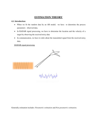
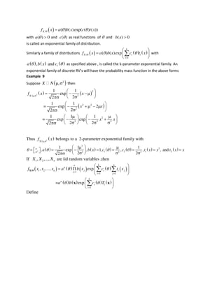
- Estimation theory involves using observed data to determine unknown parameters of a system. This includes problems like estimating locations/velocities from radar signals or inferring transmitted signals from received noisy data.
- Estimation includes parametric estimation, which assumes a model and estimates parameters like mean/variance, and non-parametric estimation, which directly estimates probability densities without assuming a model.
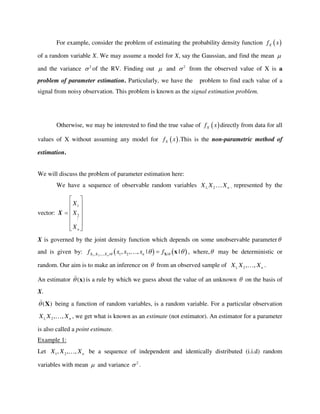
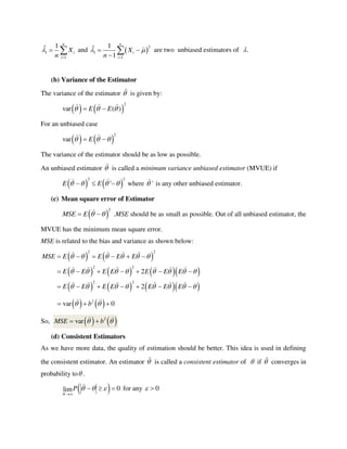
- An estimator is a rule for guessing the value of an unknown parameter based on observed data. Good estimators are unbiased, have low variance, are consistent as more data is observed, and have minimum mean squared error. The minimum variance unbiased estimator is preferred.
![Less rigorous test is obtained by applying the Markov Inequality
2
2
E
P
If is an unbiased estimator [ 0b ], then varMSE .
Therefore, if
2
0lim
N
E
, then will be a consistent estimator.
Also, note that 2
varMSE b .
Therefore, if the estimator is asymptotically unbiased (i.e. 0b as n ) and var 0
as n ,then 0MSE .Therefore for an asymptotically unbiased estimator , if var 0
asn , then will be a consistent estimator.
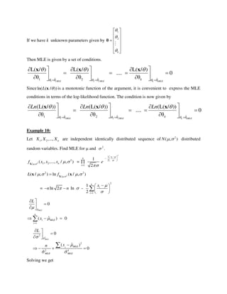
Example 3
Suppose 1 2, , , nX X X is an i.i.d. random sequence with unknown x and known 2
x .
Let
1
1 n
i
i
X
n
be an estimator for x . We have already shown that x is unbiased. also,
2
var
n
. Is it a consistent estimator?
Clearly,
2
var 0lim limx
n n n
. Therefore, is a consistent estimator of .
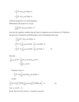
Efficient Estimator
Suppose 1 and 2 be two unbiased estimator of the parameter . The relative efficiency of the
estimator 2 with respect to the estimator 1 I s defined by
1
2
var( )
ˆvar( )
Relative Efficiency
](https://image.slidesharecdn.com/estimationtheory1-151213044648/85/Estimation-theory-1-6-320.jpg)
![/ /1 1
, ,..., /1 2
, ,..., /1 2
/
/
2 2
1 2
2
1 2
2
1 22
2
2
1
2
2
( ) ln( ( )) ln( ( ))
( ) ln( ( , ,..., / ))
ln( ( , ,..., / ))
ln( ( / ))
ln(
X X
X X Xn
X X Xn
Xi
Xi
n n
n
n
i
i
I E f x E f x
I E f x x x
E f x x x
E f x
E f
1
1
( / ))
( )
n
i
i
x
nI
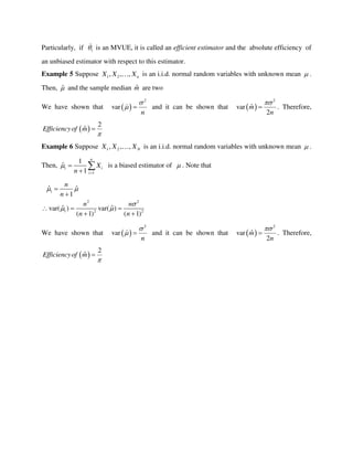
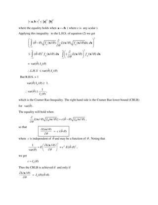
(3) If ˆ satisfies CR -bound with equality, then ˆ is called an efficient estimator.
Extension to Vector Parameters
Suppose 1 2, ,..., k are k parameters which are represented as the vector 1 2[ ... ]k θ .
Then the log-likelihood function is given by
/ 1 2( / ) ln ( , ,..., )nL f x x x X θx θ
We can represent the 1st
-order partial derivatives of ( / )L x θ as
1 2
( / ) ( / ) ( / )... ... ( / )
k
L L L L
x θ x θ x θ x θ
θ
The Fisher Information matrix is given by
( / ) ( / )E L L
nI x θ x θ
θ θ
where E is performed on each term of the matrix.
It can be shown that](https://image.slidesharecdn.com/estimationtheory1-151213044648/85/Estimation-theory-1-13-320.jpg)
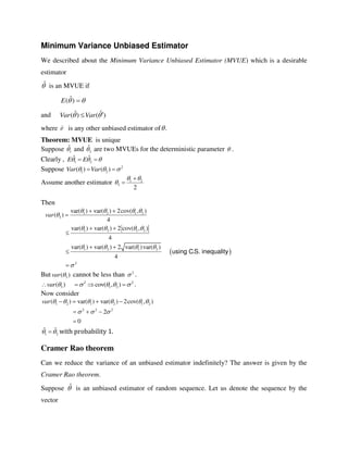
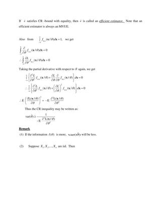
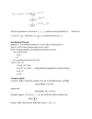
![The likelihood function / 2( , ,...., / )nf x x x X 1 will be product of individual densities (since iid)
/ 2 n
1 2( )
22 11
( , ,....., / )
( (2 )
n n
n
xi
if x x x e
X 1
so that 2
2
1
1
( / ) ln( 2 ) ( )
2
n
n n
i
i
L x
X
Now
2
1
2
2 2
2
2 2
1
0 - ( -2) ( )
2
n
-
n
So that E -
n
i
i
L
X
L
L
CR Bound =
2
2
2
2
1 1 1
( )
-n
nLI n
E
2 2 2
1
1
ˆ( ) - ( - )
2
n
i
i
i i
L n X n
X
n
estimator.efficientanisˆand
)-ˆ(c-Hence
L
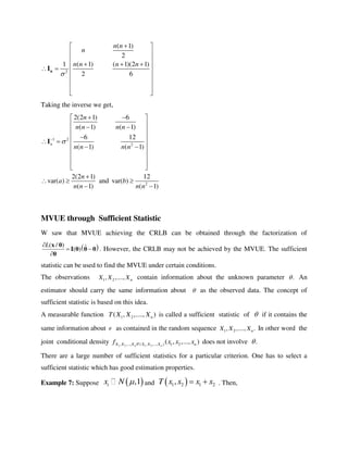
Example 4 Suppose n nX a bn V , 2
~ (0, ), and are known constants.nV N a b Here
[ ]a b θ . The -likelihood function is given by
1
/ 1 2 n
1 2( )
21 2( , ,..., )
( (2 )
i
i
n n
n
x a bi
f x x x e
X θ
2
2
1
2 2
1 1
2 2 2
2 2 2 2 2
1
( / ) ln( 2 ) ( )
2
1 1
( ), ( ) ,
( 1) ( 1)(2 1)
, and
2 6
n
n n
i
i
n n
i i
i i
L x a bi
L L
x a bi x a bi i
a b
L n L n n L n n n
a a b a
x θ](https://image.slidesharecdn.com/estimationtheory1-151213044648/85/Estimation-theory-1-15-320.jpg)
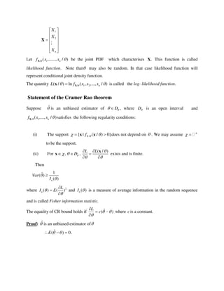
![Proof: Denote the value T(x) by t. Suppose T(X) is a sufficient statistic. Then,
: ( )
( ) ( )
( , ( ) )
( ( ) ) ( ( ) , )
( ( ) ) ( ( ) ) [ ( ) is a sufficient statistic ]
( ) ( )
( , )) ( )
T t
p P
P T t
P T t P T t
P T t P T t T
p h
g t h
X
X
x x
x X x
X x X
X X x X
X X x X X
x x
x
where
: ( )
( , ) ( )
T t
g t p
X
x x
x and ( ) ( ( ) ))h P T t x X x X
Conversely, suppose ( ) ( , )) ( )p g t h X
x x . Then,
: ( )
: ( )
: (
, ( )
( )
( )
( )
( , ) ( )
( , ) ( )
( , ) ( )
( , ) ( )
( )
( )
T t
T t
T t
P T t
P T t
P T t
P
P T t
g t h
g t h
g t h
g t h
h
h
x x
x x
x x)
X x X
X x X
X
X x
X
x
x
x
x
x
x
which does not depend on θ.
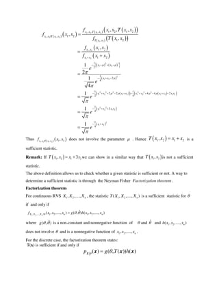
Example 8: Suppose 1 2, ,..., nX X X are iid Gaussian random variables with unknown mean
and known variance 1.
Then
n
i
i 1
1
( ) XT
n
X is a sufficient statistic of .
Because](https://image.slidesharecdn.com/estimationtheory1-151213044648/85/Estimation-theory-1-18-320.jpg)
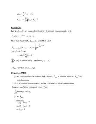
![Criteria for Estimation
The estimation of a parameter is based on several well-known criteria. Each of the criteria tries
to optimize some functions of the observed samples with respect to the unknown parameter to be
estimated. Some of the most popular estimation criteria are:
Maximum Likelihood
Minimum Mean Square Error.
Baye’s Method.
Maximum Likelihood Estimator (MLE)
Suppose 1 2, ,..., nX X X are random samples with the joint probability density
function 1 2, ,..., / 1 2( , ,..., )nX X X nf x x x which depends on an unknown nonrandom
parameter .
/ 1 2( , , ..., / )nf x x x X is called the likelihood function. If 1 2, ,..., nX X X are discrete,
then the likelihood function will be a joint probability mass function. We represent
the concerned random variables and their values in vector notation by
1 2[ ... ]nX X X X and 1 2[ ... ]nx x x x respectively. Note that
/( / ) ln ( / )L f Xx x is the log likelihood function. As a function of the random
variables, the likelihood and log-likelihood functions are random variables.
The maximum likelihood estimator ˆ
MLE is such an estimator that
/ 1 2 / 1 2
ˆ( , ,..., / ) ( , ,..., / ),n MLE nf x x x f x x x X X
If the likelihood function is differentiable with respect to , then ˆ
MLE is given by
MLE
ˆ/ θ
( / ) 0f
X x
or 0
θ
)|L(
MLEθˆ
x
Thus the MLE is given by the solution of the likelihood equation given above.](https://image.slidesharecdn.com/estimationtheory1-151213044648/85/Estimation-theory-1-23-320.jpg)


![[DSC Europe 25] Raul Cruz Bonilla - Harnessing GEN AI in Fashion, Luxury and ...](https://cdn.slidesharecdn.com/ss_thumbnails/me7nvup5thwqzwzblbvw-raul-cruz-harnessing-ai-en-luxury-260123083019-32ac5a43-thumbnail.jpg?width=640&height=640&fit=bounds)


