Download as PDF, PPTX

![Arthur CHARPENTIER, Advanced Econometrics Graduate Course
Preambule
Assume that y = m(x) + ε, where ε is some idosyncatic impredictible noise.
The error E[(y − m(x))2
] is the sume of three terms
• variance of the estimator : E[(y − m(x))2
]
• bias2
of the estimator : [m(x − m(x)]2
• variance of the noise : E[(y − m(x))2
]
(the latter exists, even with a ‘perfect’ model).
@freakonometrics 6](https://image.slidesharecdn.com/econometrics-2017-graduate-3-170307195537/85/Econometrics-2017-graduate-3-6-320.jpg)


![Arthur CHARPENTIER, Advanced Econometrics Graduate Course
Terminology
Consider a dataset {yi, xi}, assumed to be generated from Y, X, from an
unknown distribution P.
Let m0(·) be the “true” model. Assume that yi = m0(xi) + εi.
In a regression context (quadratic loss function function), the risk associated to
m is
R(m) = EP Y − m(X)
2
An optimal model m within a class M satisfies
R(m ) = inf
m∈M
R(m)
Such a model m is usually called oracle.
Observe that m (x) = E[Y |X = x] is the solution of
R(m ) = inf
m∈M
R(m) where M is the set of measurable functions
@freakonometrics 14](https://image.slidesharecdn.com/econometrics-2017-graduate-3-170307195537/85/Econometrics-2017-graduate-3-14-320.jpg)
![Arthur CHARPENTIER, Advanced Econometrics Graduate Course
The empirical risk is
Rn(m) =
1
n
n
i=1
yi − m(xi)
2
For instance, m can be a linear predictor, m(x) = β0 + xT
β, where θ = (β0, β)
should estimated (trained).
E Rn(m) = E (m(X) − Y )2
can be expressed as
E (m(X) − E[m(X)|X])2
variance of m
+ E E[m(X)|X] − E[Y |X]
m0(X)
2
bias of m
+ E Y − E[Y |X]
m0(X)
)2
variance of the noise
The third term is the risk of the “optimal” estimator m, that cannot be
decreased.
@freakonometrics 15](https://image.slidesharecdn.com/econometrics-2017-graduate-3-170307195537/85/Econometrics-2017-graduate-3-15-320.jpg)
![Arthur CHARPENTIER, Advanced Econometrics Graduate Course
Mallows Penalty and Model Complexity
Consider a linear predictor (see #1), i.e. y = m(x) = Ay.
Assume that y = m0(x) + ε, with E[ε] = 0 and Var[ε] = σ2
I.
Let · denote the Euclidean norm
Empirical risk : Rn(m) = 1
n y − m(x) 2
Vapnik’s risk : E[Rn(m)] =
1
n
m0(x − m(x) 2
+
1
n
E y − m0(x 2
with
m0(x = E[Y |X = x].
Observe that
nE Rn(m) = E y − m(x) 2
= (I − A)m0
2
+ σ2
I − A 2
while
= E m0(x) − m(x) 2
=
2
(I − A)m0
bias
+ σ2
A 2
variance
@freakonometrics 16](https://image.slidesharecdn.com/econometrics-2017-graduate-3-170307195537/85/Econometrics-2017-graduate-3-16-320.jpg)
![Arthur CHARPENTIER, Advanced Econometrics Graduate Course
Penalty and Likelihood
CP is associated to a quadratic risk
an alternative is to use a distance on the (conditional) distribution of Y , namely
Kullback-Leibler distance
discrete case: DKL(P Q) =
i
P(i) log
P(i)
Q(i)
continuous case :
DKL(P Q) =
∞
−∞
p(x) log
p(x)
q(x)
dxDKL(P Q) =
∞
−∞
p(x) log p(x)
q(x) dx
Let f denote the true (unknown) density, and fθ some parametric distribution,
DKL(f fθ) =
∞
−∞
f(x) log
f(x)
fθ(x)
dx= f(x) log[f(x)] dx− f(x) log[fθ(x)] dx
relative information
Hence
minimize {DKL(f fθ)} ←→ maximize E log[fθ(X)]
@freakonometrics 18](https://image.slidesharecdn.com/econometrics-2017-graduate-3-170307195537/85/Econometrics-2017-graduate-3-18-320.jpg)
![Arthur CHARPENTIER, Advanced Econometrics Graduate Course
Penalty and Likelihood
Akaike (1974) A new look at the statistical model identification observe that for n
large enough
E log[fθ(X)] ∼ log[L(θ)] − dim(θ)
Thus
AIC = −2 log L(θ) + 2dim(θ)
Example : in a (Gaussian) linear model, yi = β0 + xT
i β + εi
AIC = n log
1
n
n
i=1
εi + 2[dim(β) + 2]
@freakonometrics 19](https://image.slidesharecdn.com/econometrics-2017-graduate-3-170307195537/85/Econometrics-2017-graduate-3-19-320.jpg)
![Arthur CHARPENTIER, Advanced Econometrics Graduate Course
Linear Regression Shortcoming
Least Squares Estimator β = (XT
X)−1
XT
y
Unbiased Estimator E[β] = β
Variance Var[β] = σ2
(XT
X)−1
which can be (extremely) large when det[(XT
X)] ∼ 0.
X =
1 −1 2
1 0 1
1 2 −1
1 1 0
then XT
X =
4 2 2
2 6 −4
2 −4 6
while XT
X+I =
5 2 2
2 7 −4
2 −4 7
eigenvalues : {10, 6, 0} {11, 7, 1}
Ad-hoc strategy: use XT
X + λI
@freakonometrics 23](https://image.slidesharecdn.com/econometrics-2017-graduate-3-170307195537/85/Econometrics-2017-graduate-3-23-320.jpg)
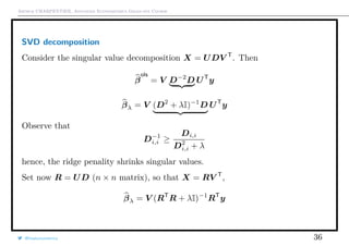
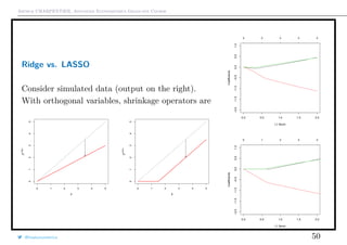
![Arthur CHARPENTIER, Advanced Econometrics Graduate Course
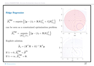
Linear Regression Shortcoming
Evolution of (β1, β2) →
n
i=1
[yi − (β1x1,i + β2x2,i)]2
when cor(X1, X2) = r ∈ [0, 1], on top.
Below, Ridge regression
(β1, β2) →
n
i=1
[yi − (β1x1,i + β2x2,i)]2
+λ(β2
1 + β2
2)
where λ ∈ [0, ∞), below,
when cor(X1, X2) ∼ 1 (colinearity).
@freakonometrics 24
−2 −1 0 1 2 3 4
−3−2−10123
β1
β2
500
1000
1500
2000
2000
2500
2500 2500
2500
3000
3000 3000
3000
3500
q
−2 −1 0 1 2 3 4
−3−2−10123
β1
β2
1000
1000
2000
2000
3000
3000
4000
4000
5000
5000
6000
6000
7000](https://image.slidesharecdn.com/econometrics-2017-graduate-3-170307195537/85/Econometrics-2017-graduate-3-24-320.jpg)
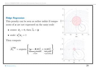
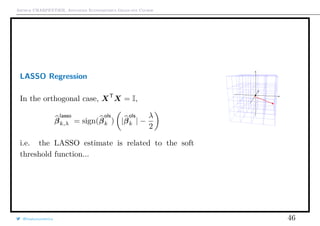
![Arthur CHARPENTIER, Advanced Econometrics Graduate Course
Ridge Regression
Observe that if xj1 ⊥ xj2 , then
β
ridge
λ = [1 + λ]−1
β
ols
λ
which explain relationship with shrinkage.
But generally, it is not the case...
q
q
Theorem There exists λ such that mse[β
ridge
λ ] ≤ mse[β
ols
λ ]
Ridge Regression
@freakonometrics 29](https://image.slidesharecdn.com/econometrics-2017-graduate-3-170307195537/85/Econometrics-2017-graduate-3-29-320.jpg)

![Arthur CHARPENTIER, Advanced Econometrics Graduate Course
The Bayesian Interpretation
From a Bayesian perspective,
P[θ|y]
posterior
∝ P[y|θ]
likelihood
· P[θ]
prior
i.e. log P[θ|y] = log P[y|θ]
log likelihood
+ log P[θ]
penalty
If β has a prior N(0, τ2
I) distribution, then its posterior distribution has mean
E[β|y, X] = XT
X +
σ2
τ2
I
−1
XT
y.
@freakonometrics 31](https://image.slidesharecdn.com/econometrics-2017-graduate-3-170307195537/85/Econometrics-2017-graduate-3-31-320.jpg)
![Arthur CHARPENTIER, Advanced Econometrics Graduate Course
Properties of the Ridge Estimator
βλ = (XT
X + λI)−1
XT
y
E[βλ] = XT
X(λI + XT
X)−1
β.
i.e. E[βλ] = β.
Observe that E[βλ] → 0 as λ → ∞.
Assume that X is an orthogonal design matrix, i.e. XT
X = I, then
βλ = (1 + λ)−1
β
ols
.
@freakonometrics 32](https://image.slidesharecdn.com/econometrics-2017-graduate-3-170307195537/85/Econometrics-2017-graduate-3-32-320.jpg)
![Arthur CHARPENTIER, Advanced Econometrics Graduate Course
Properties of the Ridge Estimator
Set W λ = (I + λ[XT
X]−1
)−1
. One can prove that
W λβ
ols
= βλ.
Thus,
Var[βλ] = W λVar[β
ols
]W T
λ
and
Var[βλ] = σ2
(XT
X + λI)−1
XT
X[(XT
X + λI)−1
]T
.
Observe that
Var[β
ols
] − Var[βλ] = σ2
W λ[2λ(XT
X)−2
+ λ2
(XT
X)−3
]W T
λ ≥ 0.
@freakonometrics 33](https://image.slidesharecdn.com/econometrics-2017-graduate-3-170307195537/85/Econometrics-2017-graduate-3-33-320.jpg)
![Arthur CHARPENTIER, Advanced Econometrics Graduate Course
Properties of the Ridge Estimator
Hence, the confidence ellipsoid of ridge estimator is
indeed smaller than the OLS,
If X is an orthogonal design matrix,
Var[βλ] = σ2
(1 + λ)−2
I.
mse[βλ] = σ2
trace(W λ(XT
X)−1
W T
λ) + βT
(W λ − I)T
(W λ − I)β.
If X is an orthogonal design matrix,
mse[βλ] =
pσ2
(1 + λ)2
+
λ2
(1 + λ)2
βT
β
Properties of the Ridge Estimator
@freakonometrics 34
0.0 0.2 0.4 0.6 0.8
−1.0−0.8−0.6−0.4−0.2
β1
β2
1
2
3
4
5
6
7](https://image.slidesharecdn.com/econometrics-2017-graduate-3-170307195537/85/Econometrics-2017-graduate-3-34-320.jpg)
![Arthur CHARPENTIER, Advanced Econometrics Graduate Course
mse[βλ] =
pσ2
(1 + λ)2
+
λ2
(1 + λ)2
βT
β
is minimal for
λ =
pσ2
βT
β
Note that there exists λ > 0 such that mse[βλ] < mse[β0] = mse[β
ols
].
@freakonometrics 35](https://image.slidesharecdn.com/econometrics-2017-graduate-3-170307195537/85/Econometrics-2017-graduate-3-35-320.jpg)
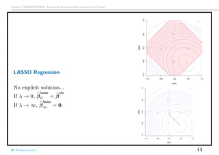
![Arthur CHARPENTIER, Advanced Econometrics Graduate Course
Hat matrix and Degrees of Freedom
Recall that Y = HY with
H = X(XT
X)−1
XT
Similarly
Hλ = X(XT
X + λI)−1
XT
trace[Hλ] =
p
j=1
d2
j,j
d2
j,j + λ
→ 0, as λ → ∞.
@freakonometrics 37](https://image.slidesharecdn.com/econometrics-2017-graduate-3-170307195537/85/Econometrics-2017-graduate-3-37-320.jpg)
![Arthur CHARPENTIER, Advanced Econometrics Graduate Course
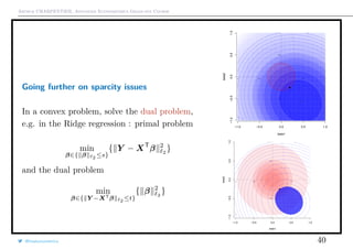
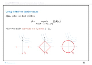
Going further on sparcity issues
On [−1, +1]k
, the convex hull of β 0
is β 1
On [−a, +a]k
, the convex hull of β 0
is a−1
β 1
Hence, why not solve
β = argmin
β; β 1 ≤˜s
{ Y − XT
β 2
}
which is equivalent (Kuhn-Tucker theorem) to the Lagragian optimization
problem
β = argmin{ Y − XT
β 2
2
+λ β 1 }
@freakonometrics 42](https://image.slidesharecdn.com/econometrics-2017-graduate-3-170307195537/85/Econometrics-2017-graduate-3-42-320.jpg)
![Arthur CHARPENTIER, Advanced Econometrics Graduate Course
Optimal LASSO Penalty
Use cross validation, e.g. K-fold,
β(−k)(λ) = argmin
i∈Ik
[yi − xT
i β]2
+ λ β 1
then compute the sum of the squared errors,
Qk(λ) =
i∈Ik
[yi − xT
i β(−k)(λ)]2
and finally solve
λ = argmin Q(λ) =
1
K
k
Qk(λ)
Note that this might overfit, so Hastie, Tibshiriani & Friedman (2009) Elements
of Statistical Learning suggest the largest λ such that
Q(λ) ≤ Q(λ ) + se[λ ] with se[λ]2
=
1
K2
K
k=1
[Qk(λ) − Q(λ)]2
@freakonometrics 47](https://image.slidesharecdn.com/econometrics-2017-graduate-3-170307195537/85/Econometrics-2017-graduate-3-47-320.jpg)
![Arthur CHARPENTIER, Advanced Econometrics Graduate Course
LASSO and Ridge, with R
1 > library(glmnet)
2 > chicago=read.table("http:// freakonometrics .free.fr/
chicago.txt",header=TRUE ,sep=";")
3 > standardize <- function(x) {(x-mean(x))/sd(x)}
4 > z0 <- standardize(chicago[, 1])
5 > z1 <- standardize(chicago[, 3])
6 > z2 <- standardize(chicago[, 4])
7 > ridge <-glmnet(cbind(z1 , z2), z0 , alpha =0, intercept=
FALSE , lambda =1)
8 > lasso <-glmnet(cbind(z1 , z2), z0 , alpha =1, intercept=
FALSE , lambda =1)
9 > elastic <-glmnet(cbind(z1 , z2), z0 , alpha =.5,
intercept=FALSE , lambda =1)
Elastic net, λ1 β 1
+ λ2 β 2
2
q
q
q
qqqqqqqqqqqqqqqqqqqqqqqqqqqqqqqqqqqqqqqqqqqqqqqqqqqqqqqqqqqqqqqqqqqqqqqqqqqqqqqqqqqqqqqqqqqqqqqqqqqqqqqqqqqqqqqqqqqqqqqqqqqqqqqqqqqqqqqqqqqqqqqqqqqqqqqqqqqqqqqqqqqqqqqqqqqqqqqqqqqqqqqqqqqqqqqqqqq
q
q
qq
q
q
qqqqqqqqqqqqqqqqqqqqqqqqqqqqqqqqqqqqqqqqqqqqqqqqqqqqqqqqqqqqqqqqqqqqqqqqqqqqqqqqqqqqqqqqqqqqqqqqqqqqqqqqqqqqqqqqqqqqqqqqqqqqqqqqqqqqqqqqqqqqqqqqqqqqqqqqqqqqqqqqqqqqqqqqqqqqqqqqqqqqqqqqqqqqqqqqqqq
q
q
q
q
q
q
q
q
q
qqqqqqqqqqqqqqqqqqqqqqqqqqqqqqqqqqqqqqqqqqqqqqqqqqqqqqqqqqqqqqqqqqqqqqqqqqqqqqqqqqqqqqqqqqqqqqqqqqqqqqqqqqqqqqqqqqqqqqqqqqqqqqqqqqqqqqqqqqqqqqqqqqqqqqqqqqqqqqqqqqqqqqqqqqqqqqqqqqqqqqqqqqqqq
q
q
q
q
q
qq
q
q
q
q
q
qqqqqqqqqqqqqqqqqqqqqqqqqqqqqqqqqqqqqqqqqqqqqqqqqqqqqqqqqqqqqqqqqqqqqqqqqqqqqqqqqqqqqqqqqqqqqqqqqqqqqqqqqqqqqqqqqqqqqqqqqqqqqqqqqqqqqqqqqqqqqqqqqqqqqqqqqqqqqqqqqqqqqqqqqqqqqqqqqqqqqqqqqqqqq
q
q
q
q
q
q
q
q
q
qqqqqqqqqqqqqqqqqqqqqqqqqqqqqqqqqqqqqqqqqqqqqqqqqqqqqqqqqqqqqqqqqqqqqqqqqqqqqqqqqqqqqqqqqqqqqqqqqqqqqqqqqqqqqqqqqqqqqqqqqqqqqqqqqqqqqqqqqqqqqqqqqqqqqqqqqqqqqqqqqqqqqqqqqqqqqqqqqqqqqqqqqqqqqqqqqqq
q
q
qq
q
q
qqqqqqqqqqqqqqqqqqqqqqqqqqqqqqqqqqqqqqqqqqqqqqqqqqqqqqqqqqqqqqqqqqqqqqqqqqqqqqqqqqqqqqqqqqqqqqqqqqqqqqqqqqqqqqqqqqqqqqqqqqqqqqqqqqqqqqqqqqqqqqqqqqqqqqqqqqqqqqqqqqqqqqqqqqqqqqqqqqqqqqqqqqqqqqqqqqq
q
q
q
@freakonometrics 48](https://image.slidesharecdn.com/econometrics-2017-graduate-3-170307195537/85/Econometrics-2017-graduate-3-48-320.jpg)
![Arthur CHARPENTIER, Advanced Econometrics Graduate Course
Optimization Heuristics
First idea: given some initial guess β(0), |β| ∼ |β(0)| +
1
2|β(0)|
(β2
− β2
(0))
LASSO estimate can probably be derived from iterated Ridge estimates
y − Xβ(k+1)
2
2
+ λ β(k+1) 1 ∼ Xβ(k+1)
2
2
+
λ
2 j
1
|βj,(k)|
[βj,(k+1)]2
which is a weighted ridge penalty function
Thus,
β(k+1) = XT
X + λ∆(k)
−1
XT
y
where ∆(k) = diag[|βj,(k)|−1
]. Then β(k) → β
lasso
, as k → ∞.
@freakonometrics 51](https://image.slidesharecdn.com/econometrics-2017-graduate-3-170307195537/85/Econometrics-2017-graduate-3-51-320.jpg)
![Arthur CHARPENTIER, Advanced Econometrics Graduate Course
Properties of LASSO Estimate
From this iterative technique
β
lasso
λ ∼ XT
X + λ∆
−1
XT
y
where ∆ = diag[|β
lasso
j,λ |−1
] if β
lasso
j,λ = 0, 0 otherwise.
Thus,
E[β
lasso
λ ] ∼ XT
X + λ∆
−1
XT
Xβ
and
Var[β
lasso
λ ] ∼ σ2
XT
X + λ∆
−1
XT
XT
X XT
X + λ∆
−1
XT
@freakonometrics 52](https://image.slidesharecdn.com/econometrics-2017-graduate-3-170307195537/85/Econometrics-2017-graduate-3-52-320.jpg)
![Arthur CHARPENTIER, Advanced Econometrics Graduate Course
Coordinate-wise minimization
Consider some convex differentiable f : Rk
→ R function.
Consider x ∈ Rk
obtained by minimizing along each coordinate axis, i.e.
f(x1, xi−1, xi, xi+1, · · · , xk) ≥ f(x1, xi−1, xi , xi+1, · · · , xk)
for all i. Is x a global minimizer? i.e.
f(x) ≥ f(x ), ∀x ∈ Rk
.
Yes. If f is convex and differentiable.
f(x)|x=x =
∂f(x)
∂x1
, · · · ,
∂f(x)
∂xk
= 0
There might be problem if f is not differentiable (except in each axis direction).
If f(x) = g(x) +
k
i=1 hi(xi) with g convex and differentiable, yes, since
f(x) − f(x ) ≥ g(x )T
(x − x ) +
i
[hi(xi) − hi(xi )]
@freakonometrics 57](https://image.slidesharecdn.com/econometrics-2017-graduate-3-170307195537/85/Econometrics-2017-graduate-3-57-320.jpg)
![Arthur CHARPENTIER, Advanced Econometrics Graduate Course
Coordinate-wise minimization
f(x) − f(x ) ≥
i
[ ig(x )T
(xi − xi )hi(xi) − hi(xi )]
≥0
≥ 0
Thus, for functions f(x) = g(x) +
k
i=1 hi(xi) we can use coordinate descent to
find a minimizer, i.e. at step j
x
(j)
1 ∈ argmin
x1
f(x1, x
(j−1)
2 , x
(j−1)
3 , · · · x
(j−1)
k )
x
(j)
2 ∈ argmin
x2
f(x
(j)
1 , x2, x
(j−1)
3 , · · · x
(j−1)
k )
x
(j)
3 ∈ argmin
x3
f(x
(j)
1 , x
(j)
2 , x3, · · · x
(j−1)
k )
Tseng (2001) Convergence of Block Coordinate Descent Method: if f is continuous,
then x∞
is a minimizer of f.
@freakonometrics 58](https://image.slidesharecdn.com/econometrics-2017-graduate-3-170307195537/85/Econometrics-2017-graduate-3-58-320.jpg)
![Arthur CHARPENTIER, Advanced Econometrics Graduate Course
Application in Linear Regression
Let f(x) = 1
2 y − Ax 2
, with y ∈ Rn
and A ∈ Mn×k. Let A = [A1, · · · , Ak].
Let us minimize in direction i. Let x−i denote the vector in Rk−1
without xi.
Here
0 =
∂f(x)
∂xi
= AT
i [Ax − y] = AT
i [Aixi + A−ix−i − y]
thus, the optimal value is here
xi =
AT
i [A−ix−i − y]
AT
i Ai
@freakonometrics 59](https://image.slidesharecdn.com/econometrics-2017-graduate-3-170307195537/85/Econometrics-2017-graduate-3-59-320.jpg)
![Arthur CHARPENTIER, Advanced Econometrics Graduate Course
Application to LASSO
Let f(x) = 1
2 y − Ax 2
+ λ x 1 , so that the non-differentiable part is
separable, since x 1
=
k
i=1 |xi|.
Let us minimize in direction i. Let x−i denote the vector in Rk−1
without xi.
Here
0 =
∂f(x)
∂xi
= AT
i [Aixi + A−ix−i − y] + λsi
where si ∈ ∂|xi|. Thus, solution is obtained by soft-thresholding
xi = Sλ/ Ai
2
AT
i [A−ix−i − y]
AT
i Ai
@freakonometrics 60](https://image.slidesharecdn.com/econometrics-2017-graduate-3-170307195537/85/Econometrics-2017-graduate-3-60-320.jpg)
![Arthur CHARPENTIER, Advanced Econometrics Graduate Course
Graphical Lasso and Covariance Estimation
We want to estimate an (unknown) covariance matrix Σ, or Σ−1
.
An estimate for Σ−1
is Θ solution of
Θ ∈ argmin
Θ∈Mk×k
{− log[det(Θ)] + trace[SΘ] + λ Θ 1
} where S =
XT
X
n
and where Θ 1
= |Θi,j|.
See van Wieringen (2016) Undirected network reconstruction from high-dimensional
data and https://github.com/kaizhang/glasso
@freakonometrics 62](https://image.slidesharecdn.com/econometrics-2017-graduate-3-170307195537/85/Econometrics-2017-graduate-3-62-320.jpg)


This document summarizes notes from an advanced econometrics graduate course. It discusses topics like model and variable selection, numerical optimization techniques like gradient descent, convex optimization problems, and the Karush-Kuhn-Tucker conditions for solving convex problems. It also covers reducing dimensionality with techniques like principal component analysis and partial least squares, penalizing complex models, and information criteria like AIC that balance model fit and complexity.


