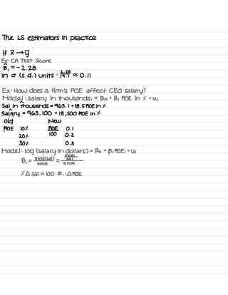
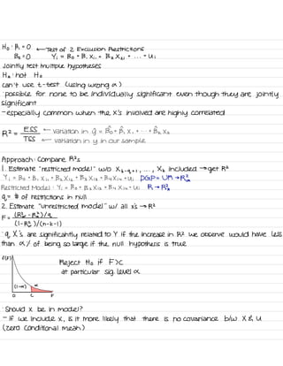
The document summarizes the Rubin causal model and key assumptions and methods for causal inference using observational data, including linear regression models. It introduces the Rubin model for causal effects, noting the need for a good counterfactual to estimate causal parameters. It then covers simple linear regression models (SLRM) and assumptions needed for causal interpretation, including the zero conditional mean assumption. 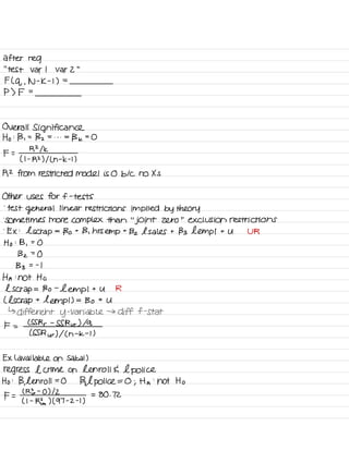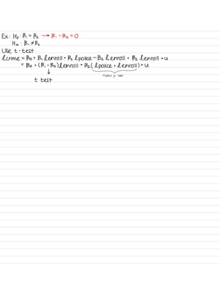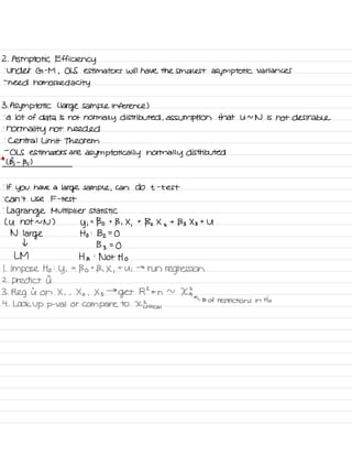Finally, it discusses multivariate linear regression models (MLRM), outlining additional assumptions required like no multicollinearity between covariates and the independence of errors from covariates. It also introduces ordinary least squares estimation and the Frisch-Waugh theorem for interpreting slope estimates from MLRM.

1. ECONOMETRICS

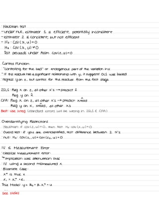
2. Recap :
.
Rubin Model :
6 =
0 + { E [ Yio 1 Ti =
1 ] -
E [ Yiolti =
0 ] }
T PaFamete#
estimator
selection effect
Assume E [ Yio IT ,
= 1 ] =
E [ Y ; o I Ti =
0 ]
↳ need good counterfactual
§ = E [ Yi 11 Ti =
1 ] -
E [ Yio 1 Ti =
0 ] if selection term = 0
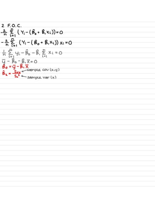
Estimating a parameter ( o )
§ =
I-
I
estimator is rule

3. Simple Linear Regression Model ( SLRM )
y ;
= Bo + 131 Xi + Ui
Bo E B 1 are parameters
U is the error term
↳
captures influence of third
party factors
$ x ; = 1 or 0
E [ Yi I X ; ] =
E [ Bo +
131 Xi +
U ; I Xi ]
=
E [ 1301 × ;] + [ [ 131 X ; l X ;] +
E [ U ; l × i ]
=
Bo +
Be [ X ; l X ; ] +
E [ Uil Xi ]
E [ Y ; 1 X ; = 1
] =
Bo + 131 + E [ U ; 1 x i
= 1 ]
-
E [ Yi 1 X ; =
0 ] =
Bo +
E [ Ui 1
X i =
0 ]
B 1 + E [ U i 1 × i =
1 ] -
E [ U ;
1
× i
=
0 ] = 131 + 0
On
average ,
unobservable s are the same
SO ATE =
131 if E [ U ; I Xi =
I ] =
E [ U i l x i
=
0 ]
Key Assumption :
Zero Conditional Mean
E [ U I X ] = 0
I . E [ UIX ] is constant *
2 .
E [ U ] = 0
implies Cov ( U , X ) =
0 ( no linear relationship )
↳ × 's are
randomly assigned
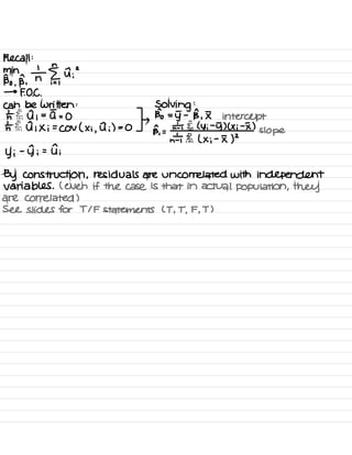
Ordinary Least Squares ( OLS )
Let { ( Xi ,
y i ) :
i =
1 , . . .
,
n } denote a random sample of size n from the
Population
Define sample estimate of the unknown population line as
yn ;
= Bo +
Be Xi
ii =
Yi
-
di and choose Bo and Be to minimize the
average squared
residual
Bone,
th En
,
( yi
-
( Bo +
BI × i ))
2

4. 2 F. 0 .
C .
-
÷ §.
,
( Y ;
-
( Bo + B. x i ) ) =
0
-
he ⇐ ,
( Yi -
( Bo + B ,
xi )) Xi =
0
then,
yi
-
Bo -
B. §,
×i=o
5
-
Bo -
B ,
I = 0
Bo =
5
-
B ,
I
B ,
=
¥4
← sample Cov ( × , y )
←
sample var ( x )

5. Recall :
min
Bo ,
R,
T §,
A ;
2
→
FOE .
can be written :
Solving
:
=
th ⇐,
d ;
=
u =
0 ,
Bo =
g -
B ,
I intercept
t.IE ,
d ; Xi =
Cov ( x ;
,
I ;) = 0
ps,
=
n÷ IF ( Yi
-
5) ( × i
-
I )
slope
n'T Fa ( × ;
-
I )
2
y ;
-
Ii = di
By construction ,
residuals are uncorrelated with independent
variables .
( even if the case is that in actual population , they
are correlated )
See slides for TIF statements ( T ,
T ,
F ,
T )

6. The LS estimators in practice
If I →
F
EI
:
CA Test Score
B ,
= -
2.28
in 0 ( s .
a . ) units :
hi?9 = 0 .
11
Ex :
HOW does a firm 's ROE affect CEO salary
?
Model :
salary in thousands ;
=
Bo +
B , ROE in % +
Ui
Sal in Thousands -
963 .
I + 18 .
SROE in %
Saiary =
963 ,
100 +
18,500 ROE in %
Old New
ROE 10% .BOE_ 0 .
I
20%
100 0 . 2
30% 0.3
Model :
log (
Salary in dollars ) =
Bo +
B. ROE i
+
Ui
2109 ( Sal )
#
B ,
= -
= sataroe 2 roe
% a Sal a 100 .
B ,
-
a ROE

7. Black vs .
White name resumes experiment
Model :
.
1 .
Callback ; = Bo + 13 .
black name ;
+
U ; ( DGP )
t
1
dummy variable ( 0 or 1 )
E [ it callback 1
black name = 1 ] =
Bo + 13 , [ black name
1
black name = 1 ] +
E [ Ul black name =L ]
=
Bo + 13 ,
+
Et Ul black name = 1 ]
t
z
Unobservable Conditional on black.name = I
E [
'
1. Callback I black name =
0 ] =
Bo +
B , E [ black name lblackname =
0 ] +
E[ Ul black name = 0 ]
=
130 + E [ U I black name = 0 ]
1 -
2 =
13 ,
+
E [ Ulblk = I ] -
E [ Ulbl 1<=0 ]
randomized experiment → left with 13 ,
13 ,
=
gap between difference in it Call back
Bo = % call back for white names
Bo + B ,
=
.
1 .
Call back for black names
Are LS estimators any good ?
.
SLR .
1 Pop . Relationship is Yi = Bo + B , Xi +
Ui
.
SLR . 2 Random Sample of × and Y from pop .
is LR . 3 There is variation in ×
-
Language :
"
our estimate of B is identified off the Variation in ×
-
denominator of B, cannot be 0
.
As SLR .
4 E [ UIX =
0 ] →
ETU ] =
0 and Cov ( U ,
X ) = 0
-
variation in × provides unbiased proxy for Counterfactual
-
produces an unbiased estimate of the causal effect E [ B, ] =
13 ,
↳
§ E [ × ;] =
M
Estimate of pop . mean =
In
E [ In ] .
-
E [ th El,
X ;] =
th E EE,
× ;] = th ¥,
E [ xi ] =
the ,
M =
M
Showed sample mean for pop .
mean is unbiased
-
will not need to replicate
Y ; =
Bo +
B , Xi +
Ui
I =
Bo +
B , I + I
Y ;
-
I = B , ( × ;
-
I ) + ( Ui -
I ) biased up or down ?
ph =
ht Et ( B ,
( Xi # ) +
( ni -5 ) ) ( × ;
-
I ) q
→ see textbook is Cov + or
-
?
's §,
( x ;
-
I ) ( x i
-
I )
T
E [ B, ] =
B ,
+
coal
bids term
→
If ZCM holds
var ( × )
then E [ B, ] =
13 ,

8. .
SLR .
S Var ( U 1 X ) =
Constant = 02
-
homos kedasti City
Prediction
.
sometimes care about ability of × to predict y
.
r ( correlation ) and its
square ,
R 2
r =
COV ( × , y ) / [ S × Sy ]
Unit free
.
s -
standard error of regression ( MSE =
sz )

9. Motivations for Multivariate Model
-
interested in effects of more than one variable on an outcome
.
refine predictions
.
If SLR .
4 is violated -
reducing committed variables bias
.
allow for some kinds of non -
linear relationships
SLRM : Yi =
Bo + B , Xi +
Ui
MLRM : Yi = Bo + B , X I ;
+
Bz Xzi +
133×3 it . . .
+
BK Xki +
Ui
k :
# of explanatory variables ( covariates , independent vars )
Yi :
dependent variable ( Outcome )
Ui :
error term ( unobserved determinants of Y )
-
linear in parameters ( B 's )
-
model Can capture non -
linear relationships with X 's
.
MLR . 2 :
simple random sample
.
MLR .
3 :
no X 's are constant ,
and no perfect linear relationship blw X 's
-
no perfect multi -
Col linearity
-
¥ =
13 , ( all else constant )
.
MLR .
4 : E ( Uil Xii ,
. . .
,
Xki ) =
0
-
independence assumption ( critical for causal inference )
-
variation of zero conditional mean assumption
-
implies COV ( Xii ,
Ui ) =
Cov ( Xz ; ,
U ) =
. . .
=
COV ( Xki ,
Ui ) = 0 E E [ U ] =
0
-
as if X 's were randomly assigned
-
If it holds ,
we
say variation in X , . . .
Xk is
good
-
provides an unbiased proxy for counterfactual
Ordinary Least Squares ( OLS )
Estimation of the MLRM
min
Bo
,
B, ,
...
Bk
T i§,
Yi
-
( Bio + B.Xii + . . .
+
Be × ,<
;)
see slides
Force Cov ( a ; ,
Xii ) = 0

10. Interpreting slope estimates in a multivariate regression
See slides
EX I :
College GPA = 1. 29 +
. 453 ns GPA + 0 .
0094 ACT
0.453 :
holding ACT constant ,
a 1
point increase in HSGPA will result in a
-453 point increase in COIGPA
EX 2 :
log (
Wage ) =
0 .
284 +0.92 educ +0.0041 exp
+ 0.022 tenure
tenure :
years at firm
0.092 :
Holding everything else constant ,
1 additional year in education will
result in 9.2% increase in
wage
dytx 100
dx
=b× 100
My =
a + b In X +
U
dlny
× 100 % Lly
A In ×
= b =
#
dx_
= -
x
× 100 % A X
elasticity
y= a + bln X +
U
b =
-04 =
dy
d In X
¥
*o
=
ay
¥ x 100
EX 3 :
p rate =
80 .
12 + S .
SZM rate +0.243
age
prate : % of people participating in pension plan
mrate : % of match rate
5. 52 :
Holding age constant , increasing match rate by It .
point will result in
increase in participation of S . SZ % points
EX 4 :
Ln ( sales ) =
130
-
2 .
1
In ( price ) +
. . . Controls
controls :
advertising cost , season
2.1 :
Holding all else constant ,
a it increase in price results in 2.1% decrease
in sales
elasticity of demand

11. Frisch -
Waugh Theorem
.
OLS estimator :
B,
=
Cov ( F, ; , y ;) 1 Var L ni )
where Fi = X ,
-
K ,
1.
Regress X ,
On Xz . . . xk ,
get residuals Fi ;
2. Regress y on residuals Fi ( bivariate )

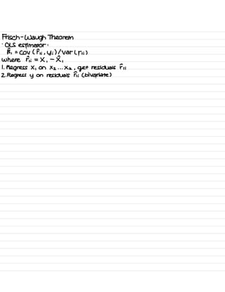
12. MLRM : Y ;
=
Bo +
B , Xi ;
+
132 Xzi + . . .
+
BKXK ; + U ;
.
Frisch -
Waugh Theorem : The OLS estimator for B, can be written as :
B,
=
COV ( Fii , Yi )
var ( F , ;)
F , ; ? from X , ;
=
do +
£2Xzi
+
£3Xz
;
+ . . .
Fii =
Xii -
Iii
Stata
Open FWL do fill in do fill editor
Open LFS data set in STATA
Desc :
describe
gen age 2 =
ager 2
sum . . .
histogram ...
reg . . .
.
0948038
predict that ,
resid
predict Xb
R squared :O . 1436 → 14.36% of variation in In wage can be explained
by included X 's
Too Many or Too Few Variables
.
include Variables that don't belong
-
no effect on our parameter estimate , OLS remains unbiased
-
lose statistical precision
.
exclude variable that doesn't belong
-
OLS is biased
-
"
omitted variables
"
bias
-
E [ BY ] = B ,
+ Bz
COV ( × ' . xz )
*
V ( X ,
)
¥
can reason about sign of Bz { covariance to estimate error

13. Summary of Direction of Bias :
Bz I ,
see table from Slides
If 132=0 ,
then no relationship btw Xz and
y
Ex :
Case and Paxson 2008
.
Correlation btw
height and earnings is positive
-
causal ? biased ?

14. On website , suggested
problems E prior midterm
Population Mean Sample Mean
if M is mean In = Tn Fei Xi
of random Variable Xi
Then Et I ] =
M
Yi =
Bo t
B , X , i
t
Bz X z i
t
. . .
t
Ui
In
Bi =
n IE ly i
-
5) ( x i
-
I )
SL RM
th I ,
( x
;
-
I 5
Sample Variance : V Tarts.
)
=
se ( Bj )
Additional Assumptions about error Variation
MLRM Assm # S :
Var( U I X ) = OZ
Homos ked asti city t
no autocorrelation
Cases where assm fails :
.
time series data
.
samples w/
"
Clusters
"
Li .
e.
survey several members of the same family )
Var ( Bj ) =
02
( N -
t ) Var (
Xj
) ( I -
Rj
2
)
Where Rj
2
is the R2 from regressing Xj on all other x 's L first part Of Frisch -
Wa USS
02 is variance ;larger
02 →
larger variance in Bj
N -
I :
need
large N to reduce variance of Bj
Var ( Xj ) :
want variance of Xj to be larger
↳
not all variance in Xj contributes to the variance in Bj because some variation
in Xj may be correlated with other X 's
( I -
Rj
'
) :
what share of variation in Xj is independent correlation
↳ would like low correlation between X 's
Large variance means less precise estimator ,
larger confidence intervals ,
E. less accurate inference

15. We don't know 02 because we don't Observe the errors ,
Ui
O
2
c- Unknown ,
estimate of
0^2
= S2 =
( ¥ ) ,
I ;
2
( Mean squared Error )
k = # of X 's included in the model
0^2 :
how much residuals vary
N -
K -
I :
degrees of freedom
Gauss -
Markov Theorem
.
Under MLR .
I -
MLR .
5 ,
it can be shown that OLS is
"
blue
"
-
Best Linear Unbiased Estimator
-
efficient ,
smallest Variation
-
with heteros ked asti city ,
this will no
longer be true
How do we determine the distribution of our estimates ?
A SSM MLR .
6 :
U I X n N ( O ,
02 )
Bj ~
N ( Bj ,
Var L Bj) )

16. Inference
.
zero conditional mean assumption
-
violated if unobservable affects both an X G Y
Assumptions I Ideal Conditions
.
MLR .
I -
4 C as before )
.
M LR .
5 :
homos Kedah city Var ( u I X ) =
02
.
MLR .
6 :
normal errors
:
U I X ~ N ( O ,
02 )
.
Under MLR .
I -
6 ,
Bj will satisfy
:
( Bj -
Bj )
Sd ( Bj )
~ N ( O ,
I )
.
Sd Unknown
↳ ( Bj -
Bj )
Se ( Bj )
~ t
N -
K -
,
( If N > 100 , very large ,
can use normal distribution )
R2 = Est =
I
-
⇒
"
↳ In Stata ,
ESS = model sum of squares
30-1 .
of the variation in output can be explained by X 's in model
"
Root Mean Squared Error I Root MS E ) : Ii Ii
Z
Variance of residual ( N -
K -
I )
RSS L residual )= -
N -
K -
I
K :
# of Slope parameters ( Model df I

17. In defect =
Bot B , training t
Stuff t
Ui
Ho :
B ,
=
O
HA:
B ,
⇒ O 2 tailed test
Significance Level :
A = . 05 P L type 1 error )
L test ) t statistic =
Bi -
B '
↳ P ( Reject Ho I Ho is true )
se ( B,
)
t
=
ji = -
z . za
% %
-
2!
2-6
-
-
t c
O
t c
Decision Rule :
Reject Ho if I test statistic I 7 It critical I for fixed x
£ 43 -
3 -
I
,
. OS Cz tailed )
=
2 .
021
2. 02672.021 →
Reject Ho
In STATA type dis in Vt tail C 39 .
0.025 )
For p
-
Val :
p
-
Val = 0.03
or
{ Ha
:B.
so }
Reject Ho iff t statistic L -
t critical for fixed a
* Never accept null :
Reject Ho or fail to reject Ho
Confidence Intervals L Regions of Non -
Rejection )
2 Sided test :
Bj ±
t critical
.
se l BI )
BT -
t c
.
Se ( Bi ) I Bo I Bj t t
c
'
Se ( Bj )
If O is outside of confidence interval , reject Ho
For One -
Tailed ,
Divide p -
Val by 2

18. Exam :
9120
8:00 -
9:15am
129 De Bart .
Bring pen
Format
75 min
100 points
~
half MC ,
half Short answers

19. Ho
:
Bi =
O
←
Test of 2 Exclusion Restrictions
132=0 Yi =
Bo t
B , Xi,
t Bz X z i
t
. . .
t
U i
Jointly test multiple hypotheses
Ha :
not Ho
can 't use t -
test L
using wrong a )
.
possible for none to be
individually significant even
though they are jointly
significant
-
especially common when the x 's involved are
highly correlated
R2 =
ESS ←
Variation in yr =
Bho t
B, X ,
t - . .
t BI Xk
TSS ←
variation in y in our sample
Approach :
Compare R2 s
I .
Estimate
"
restricted model
"
W/O Xk -
q + , ,
. . .
,
Xk included →
get R2
Y i
=
Bo t
B , Xi ,
t
Bz X iz
t
Bz X is
t
By Xi 4
t U ; DGP = UM →
RE.
Restricted Model :
Yi = Bo t
B s
X is
+
By Xiu t
Ui R →
Rk
of
=
# of restrictions in null
2. Estimate
"
unrestricted model
"
w/ all x 's → R2
F =
l Mur -
RL ) Iq
( I -
RE ) I ( h -
k -
I
)
-
q X 's are
significantly related to Y if the increase in R2 we observe would have less
than a % of being so
large if the null hypothesis is true
f (F)
Reject Ho if F > C
at particular Sig . level or
↳( I -
a )
O C F
-
Should X be in model ?
-
If we include X ,
is it more likely that there is no covariance btw X E U
( zero conditional mean )

20. after reg
' '
test var I var 2
"
F ( q ,
N -
K -
I ) =
P ) F =
Overall Significance
Ho :
B ,
=
Bz = . . . =
Bk =
O
F =
R 21k
( I -
R2 ) I L n -
k -
t )
R2 from restricted model is 0 b/c no Xs
Other uses for f -
tests
.
test
general linear restrictions implied by theory
.
Sometimes more complex than
"
joint zero
"
exclusion restrictions
.
EX :
l scrap
=
Bo t
B ,
hrs empt Bz l sales t Bs hemp I t U UR
Ho : B ,
=
O
Bz =
O
Bs = -
I
HA :
not Ho
l scrap = Bo -
Lemp I t U R
( l scrap t
tempt ) =
Bo t
U
↳ different y
-
variable → diff f -
Stat
F =
CSS Rr -
SS Rur ) la
( SSR ur ) I ( h
-
k -
I )
EX l available on Sakai )
regress l crime on Len roll E l police
Ho :
B,
l enroll =
O
Bal
police = O ; Ha
:
not Ho
F =
( RE -
O ) 12
( I -
Rfra ) ( 97 -
z -
I ,
= 80 . 72

21. EX :
Ho : B ,
=
Bz →
B ,
-
B z
=
O
H A
:
B , ¥Bz
Use t -
test
l crime =
Bo t
B , l enroll t
Bz l police
-
Bz l enroll t
Bz Len roll t
u
.
-
Bo t ( B ,
-1132
) Leh roll
t
Bz
(ll
) t
U
new x var
t test

22. Asymptotic
Unbiased ? Et B ] =
B
Smallest variance : B is BLUE
U n
N → B ~
N ( B ,
V ( B ) )
-
testing
-
Asymptotic :
Can we still
get good estimators with weaker assms ?
Takeaways
Small Sample Large Sample *
LS estimators are . . .
I
.
Consistency
.
an
'
.
estimator
"
is consistent if
pl im
n → as
B' →
B
If n
gets larger ,
going toward population
-
under Gauss -
Markov as Sms
, Slope estimates are consistent
-
B can be biased for small n and consistent in large samples
Suppose pie = I t th
E I A] =
M t th As n → as
,
ht
goes to O
.
For unbiased ness :
need E EU I X , , Xz ,
X .
T =
O assm to hold in small sample
.
For consistency ,
only need E EU 7=0 and COV ( u ,
X ) =
O

23. 2 . Asmptotic Efficiency
.
Under G -
M
,
OLS estimators will have the smallest asymptotic variances
-
need homos ked a city
3. Asymptotic C
large sample inference )
.
a lot of data is not normally distributed , assumption that U ~
N is not desirable
.
normality not needed
.
central Limit Theorem
-
OLS estimators are
asymptotically normally distributed
*
( Bj -
Bj )
.
If
you have a
large sample ,
can do t -
test
.
can 't Use F -
test
.
Lagrange Multiplier statistic
( U not NN )
y i
=
Bo t
B ,
X
,
t
Bz X
z
t
133 X 3
t U
N
large Ho :
Bz =
O
I
133=0
L M Ha :
Not Ho
I
.
impose Ho :
y i
=
Bot B , X ,
t
Ui
→
run
regression
2. predict I
3 .
Reg it on X , ,
X z .
X 3
→
Get
RZ * n
~
Xk
T # of restrictions in Ho
4 .
LOOK up p
-
Val Or compare to X Eri tical

24. Readings : Ch 6 ,
7
↳ practice problems at end
Specification Choices
'
ML RM is
"
linear
"
in parameters
-
measuring x 4 y
in
logs
-
data scaling
-
polynomials
-
dummy variables
-
etc .
-
Polynomials for non -
linear ities
Ln L wage ) .
-
Bo t
B ,
yrs ed t
Bz potexpt 133 pote Xp
2
the
pot exp
=
age
-
edu -
6
01h
wage
2 pot exp
=
Bz t
2133 Pote Xp
I t
also captures main 2nd order
effect of aging effect effect
pot exp
.
-
21 →
mean marginal effect =
Bz t
2133 C 21 )
Reaches Max or min slope at potexp =
-
132/2133
↳
Find using Bz t
2133 pot exp
=
O
Stata : fun with dummies
*
main effect :
Holding all else constant E pot exp
= O →
Dummy Variables
-
2 Values only
{ O ,
I }
'
Mean of dummy variable :
X ,
=
I female I =
In II ,
Xi = share of 1 's
0 male
.
Dummy in regression
Yi
= Bo t
So do +
B , Xi t
Ui Where do = I or O
E I y
I
do =
I ] =
( Bo t
So ) t
B , X i
t
E EU I do =
I ]
E I y
I do = I ] =
Bo t
B , Xi t
Et U I do ] =
O
I
Et y
I
do =
I ] =
( Bo t
So ) t
B , X i
t
E EU I do =
I ]
E I y
I do = I ] =
Bo t
B , Xi t
EE U I do ] =
O
So Et y
I do =
I ] -
E t y
I do =
O ] =
So

25. I
.
dummy for intercept shifter
2. dummy for Ll 's over time
3 .
dummy for multiple categories
4 .
dummy variable interactions
.
time dummy
A t
'
-
I if year
=
2009
O if
year
=
2008
y t
.
-
I if
unemployed
O if not
DGP :
ye
=
Bo t
ft d t t
Ut
Et ye Idt = I ] =
Bo t
St t
EE Ut Id +
=
I ]
E Eye Idt =
O ] =
Bo t E t Ut I de
=
O ]
Under ZCM : E E Ut Id t
=
IT =
Et Ut Idt =
O ]
E
Eye I d t
=
I ] -
E I
y t
I d t
=
03 =
St
Diff in
unemployment over time
-
Multiple Category Dummy
-
cannot include all
categories ,
must omit base
category
-
constant is
avg y ,
conditional on all other variables being O
Yi =
Bo t
B ,
NE t Bz MW t
Bs Sth t
Ui
Et Yi
I NE =
0 ,
MW =
O ,
Sth =
03 =
Bo . . .
average y for base I omitted cat .
( west )
E Ty i I NE =
O ,
MW = I
,
Sth =
O ] =
Bo t
Bz =
average y for MW = I
( B -
A ) =
B 2
E E
y
I Sth = I
,
MW = O ,
NE =
OT =
Bot Bs
( Sth -
MW ) =
133 -
Bz
Yi =
Bo t
B ,
NE t Bz MW t
Bs Sth t
By
yrs ed t
y i

26. Dummies Continued
.
preview
-
include M -
I
categories of dummies
-
fixed effects are another name for dummies
-
interpretation
:
coefficient of
dummy variable is effect in relation to omitted category
-
changing slopes
Yi
=
Bo t
So do t
B , Xi t
U i
y i
=
Bo t
So do
+
B , X i
t
8 ,
do *
X i
t
Ui
E I y i I do =
I ] =
Bo t
So t
B , Xi t
8 ,
X i
=
( Bo t
8 o ) t
( B ,
t 8 ,
) X i
E t y i
I
do =
O ] =
Bo t
B , Xi
y
=
Bo t
Bi NE t Bz MW t 133 Sth t 134 yrs ed t
Bs N E *
yrs ed t
136MW *
yrs ed t 137 Sth *
yrs ed t
U
E [ y
I N E =
O , MW =
O ,
Sth =
OT =
Bo t
134
yrs ed
↳
main effect , slope for committed group
E t y
I NE = I
,
MW =
O ,
Sth =
O ] =
Bo t
Bi t 134
yrs ed t
Bs yrs ed
=
( Bo t Bi ) +434 t
Bs )
yrs ed
E I y
I NE ,
MW ,
Sth =
IT =
Bot 133 t ( B 4
t 137 ) yrs ed
-
EE Y
I NE ,
MW =
I
,
Sth =
I ] =
Bo t
Bz t
( 134 t Be ) yrs ed
( 133 -
Bz ) t
( By -
B 6) yrs ed
.
Diff in returns to edu in NE VS .
Sth
:
B s
-
B >
= -
. 0117
-
.
018
Chow Test
H o
:
B ,
=
132=133 =
Bs =
136 =
By =
O
R ? :
y i
=
Bo t
134 yrs ed t
U
H A
:
not Ho
can use f -
test or Chi squared test L use f -
test here )
( R Ir -
Rim ) 19
~ F
( I -
RE r ) KN -
k -
t )
Will probably fail to reject null in this case
In this sample ,
not significant difference in terms of return to education
.
Interactions of continuous variables
Ln L
wage ) =
Bo t B , yrs ed t
Bzpotexpt Bs pot exp
*
yrs ed t
U
Partial derivative interpretation
:
2 In
wage
2 yrs ed
=
B ,
t
Bs pot exp

27. Deviations
!
-
heteros ked asti
city ( HT SC )
V ( U I X ) ¥ 02
-
V ( U I X ) =
02 ( X )
.
Variance of u is different for different values of X
.
ex :
estimating returns to education
-
more variation at
higher levels of education than for high school dropouts
.
other examples
-
If Y data are sample means
I data
Var ( T ) =
' )
=
I
N
If N 's are different for each Sample → HTS C
-
If Y is a
dummy dependent value
.
consequences
-
OLS is still unbiased and consistent
-
standard errors are biased
-
can 't use t
-
statistics ,
f -
statistics ,
or LM -
statistics
-
regular OLS is not efficient
-
weighted least squares is efficient
Ex i
20 ? Exit ? * Don 't have to memorize
Var ( B,
)=fz×py2
→
I Exp ]
'
* use robust in STATA
'
Robust Standard Errors
-
biased in small samples ,
but consistent
-
will not have t .
dist
-
robust se
may
be smaller or
larger than regular se
*
Always use robust !
Might have heteros ked asti
city .
-
HOW do you know it you have heteros ked asti city ?
Ho :
E I U2 I X ] .
-
02 = V L u I X )
HA :
not Ho
I
.
Regress y i on Xi → Ii for all i
^
.
2
2 .
U ,
3 .
Reg is ? on Xi 's →
test ?
↳
test joint
-
significance of all Bs in step 3 using f -
test or LM -
test
Reject ? not homos ked -
Fail to reject ? homos ked .
is ok

28. I ;
=
y i
-
Yi =
Yi -
Bo -
Bi X ,
.
BP test :
will detect linear forms of homos ked .
.
White test allows for nonlinear ites
↳ see slides
Weighted Least Squares →
for y as sample means
-
Var ( Ic ) = II ,
data set of cities
T
sample means
Yc =
Bc I c
t
Uc larger cities →
more accurate info on
wages E pop .
immigrant
Transform data to eliminate source of HTSC
hi = Ntc
Jc =
B Ic t
U
Tnc Jc = B TN c Ic t
TNT .
u
-
New model
5 c
=
B Ic t VTc
Var ( 5 c) =
Var L Tnc .
5 c ) =
Nc Var ( 5 c ) =
Nc
.
two =
OZ
BY
WLS
=
E Nc Jc Ic
E Nc XI
.
STATA :
reg y x t -
=
weight I
Measurement Error
-
recall error
.
respondent error
.
Social desirability bias
.
Does this lead to bias in LS estimators ?
.
Measurement error in
y
-
*
=
' '
truth
"
non * =
actual data
Yi =
y i
* t
e i o

29. -
classical measurement error :
E Elio ] =
O
And COV Lei o ,
Xi ) =
O
COV ( e ,
-
o , y ;
*
) =
O
-
Implications :
True Model :
y
* =
Bo t
B , X ,
t
Ui
y
* t
Cio =
Bot B , Xi t
L U i t e i o )
What I can
get
:
y i
= Bo t
Bi X ,
t
( Ui te ; o )

30. Classical Measurement Error in X
§ Xi =
Xi
*
t
e it
T T T
actual data truth error
C. M .
E .
AsSms ; e is Uncorrelated with Ui and Xi
*
We want :
y ;
=
Bo t
B , Xi
*
t
Ui
← well -
behaved error
we can
get
:
Yi
=
Bo t B ,
( Xi
-
eis ) t
Ui
=
Bo t
B , Xi
-
B ,
e i ,
t
Ui
=
Bo
t
B , Xi t
( Ui
-
Bie it
)
n n
U ;
*
COV ( Xi ,
Vi
*
) ± O
So what ?
Et Bus ] * B but we can derive in what
way it differs
pl im
Big =
COV ( Y ,
× )
=
COV ( Bot B , Xt Ui
*
.
X )
=
B ,
V L x )
+
Cov ( Ui
*
, Xi )
var CX ) Var CX ) V L X ) v ( x )
COV Lui
*
, Xi )
=
COV ( Ui
-
B , ei , Xi
*
t em ) =
CoV ( -
B , Ei ,
ei )
=
-
Bi V Lei ) CME
V ( Xi ) V ( Xi ) V C Xi ) V ( Xi ) ASSMS
Him L B,
) = B , ( o
,⇐?¥z ) Weighting the truth that the estimate is able to tell us
T
MUST be less than I
Always closer to 0 than it Should be
Adding more X 's →
reducing signal signal t
noise
↳
other Slope estimates are biased ,
but not in predictable ways
Can it be fixed ?
'
Using administrative data to find Oe
'
-
see slides

31. More Data Problems
-
difficult -
to
-
observe variables
-
use observable
"
proxies
' '
-
ability
→
IQ score
-
quality of school →
student -
teacher ratio
-
impact depends on which way proxy is used
* -
treatment variable
-
controls
.
Missing Data
-
If data is
missing at random ,
not a problem
-
If data is missing systematically L i. e. high income individuals refuse to provide
income data ) →
violates MS L it
.
Nonrandom Samples
-
selected on X is ok
-
selected on
y or U will lead to bias
-
outliers
-
can be data
entry problem
-
or can be an X or
y that looks different
-
Winsor ize data I trim
-
drop data by looking at
sensitivity
-
least absolute deviations CLAD )
-
look at relationship btw X G y at the median
-
STATA :
greg
-
quantile regression

32. Panel Data and Methods
'
Differencein difference
-
use interaction of time dummy Variable with another
dummy variable
-
can sometimes help get at causal effects
-
Research question :
What's the impact of more immigrants on native unemployment
rates ?
-
issues w/ cross-sectional data ?
-
sorting of immigrants ( higher unemployment rates in cheap cities )
.
EX :
Mariel boat lift
-
natural developments
-
Apr
-
Oct 1980 :
100,000 Cubans poured into Miami ( 60,000 Stayed )
-
compare changes in unemployment rate 1979 -
1981 in Miami to
changes in
"
comparison
cities
"
Yi =L if
unemployed
O if not
D= unemployment rate
Gg
=
change in
unemployment rate
( y-m.tt ,
-
Tm , t
) -
( Dc ,
t ti
-
5 c
,
t
)
- -
treated Controlled
2 Dummy Variables
Di
Miami
=
{
I Miami
D;
1981
=
{
I after boat lift ( 1981 )
O
comp cities O before boat lift 4979 )
Yi =
Bo t
B ,
D ,
Miami t
y ;
B ,
:
difference between employment rate in Miami and different cities
Yi =
Bo t
B , Dimiamit Bz Dila
' '
t
133 Di
Miami .
Di
1981
t
U ;
Bz :
Change in employment rate from 1979 -
1981 in comparison cities
E [ Yi I Di M =
I ,
Di
' 98 '
= I ] =
Bot B ,
t Bz t Bs
-
Et Yi I Di
M = I
,
Di
'
981=0 ] =
Bot B ,
Bz t
133 If B ,
=
O , helpful
Diff in Whom ploy .
L no diff .
b/w whomp .
btw
btw 81 E 79 in M cities in 1979 )
Et Yi I
Di
M
=
O
,
Di
' 98 '
=
I ] =
Bo t
Bz
-
Et Yi I Di
M -
-
O
,
Di1981=0 ] =
Bo
Bz
Change in vnemptoy .
in
comp .
cities pre to post
( Bz t
Bs ) -
Bz =
133
how much larger was the change in when ploy .
rate in Miami than in comp . Cities

33. -
"
Generalized
"
diff in diff
Yi =
Bo
t
B , Di
M
t
Bz Di
' 98 '
t
Bs Di M .
Di
' 98 '
t
134 yrs ed t
Ui
controlling for Other info
.
panel Data
-
time series G cross -
sectional components
-
same people ,
firms ,
households over time
-
can be used to address some kind of omitted Variable bias
-
If omitted Variable is fixed over time , a
"
fixed effect
"
approach removes bias
y it
=
Bo t
So d 2 t
t
B , X it I
taitUit_
I V it
time -
constant component of the
composite error ,
v
ai :
person
-
effect ( etc . ) has no
' '
t
' '
Subscript →
fixed over time
↳
ability ,
risk
adversity
U it
:
idiosyncratic error
Both ai and Vit are unknown errors
If ai Corr .
W/
any x ,
OLS will be biased
Controlling for Fixed Effects
.
Introduce a dummy variable for each individual ,
i
↳
only include m -
I
categories
Differencing Out Fixed Effects
Per . 2 :
y
iz
=
Bo t 8 o
.
I t
B ,
X iz ,
t . . .
t
Bk Xizk
t
di t
Viz
Per I :
y i ,
=
Bo +8 o
.
O t
B , Xi it
t . . .
t
Bk X i ik
t
dit Uil
Diff :
Ll
y i
=
So t
B ,
DX t . . .
t
Bk 4k t
I Ui

34. Unobserved F. E .
Models
,
fixed effect
y it
=
Bo t
So d t
t
B , X , it
tditU
Problem :
Is COV ( Xi it , di ) t
O
↳
OV B or biased estimator
↳
autocorrelation ( Corr ( UFT .
Viz ) ¥0 )
I
Standard errors are wrong
Eliminating F. E .
or
xtreg ,
fe
.
adding dummy variables for a i
↳
controls everything that is fixed over time
.
differencing
.
demeaning data
Differencing :
y iz
=
Bo
t
So *
I +
B ,
X i iz ta i
t
U iz
-
y it
=
Bo t
So *
O t
B , X , i i
t
a ;
t
Wiz * shrink data set by half
*
mathematically equivalent to
y i
=
So t
B ,
I Xi i
t
Qui adding in dummies when
only
←
COV ( a Xii ,
Qui ) =
O
2
years
Crmrte
⇐
=
Bo t
So d E
'
t
B. Unama tac t
Uct
Q n
:
Cov Currence ,
a
c I =
?
Demeaning Data
y it
= Bo B I X it I
t . . .
t
di t
U it
Per I :
y it
=
Bo t Bi X it I
t . . .
di t
Ui I
Mean :
YT =
Bo t
B , Ii ,
t . . .
ta i
t
UT
( y it
-
YT) =
B , ( Xii
-
Ii ) t . . .
t
( Uil -
UT ) for each i ,
t
General FE estimator :
( y it
-
g- i ) =
Bi L X it ,
-
Iii ) t
L Uit
-
UT )

35. Recall :
Unobserved F. E .
Model
y it
=
Bo t
So d t
t
Bi X , it
t
a i
t
Uit
-
unobserved part
Is Cov ( X it .
A i ) =
O
4 i induces serial correlation of error terms → violates MLRM .
5
,
no
longer efficient
If heteros kedasti city ,
then inference is
wrong .
↳
robust L new formula for se . )
↳
weighted Least squares ( new formula for estimate )
↳
weight up observations that have smaller error variance
, weight down for
observations w/
large error variance
↳
e. g .
data is sample means
If autocorrelation →
Cov Cutie .
U ) # O t t €
j
U it
*
=
X i
t U it
↳
inference is
wrong
estimates become
↳ clusters .
e . In STATA :
reg crmrte Ipo Ipc ,
cluster C area ) less precise ,
Ses
larger
↳ random effects
Estimating F. E. s in STATA
1.
Adding dummies Xi :
reg y x i. group var
2 .
Absorb :
a
reg y X
,
absorb L group var )
3 .
Xtreg
↳
xtset
↳
xtreg y x ,
fe
between VS .
within ;
taking out firm fixed effects
Fat rates t
=
Bo t
So dt t
B ,
Beer tax s t
t
as
t
Ust
First difference :
Fat rates z
=
Bot So t
B , Belttaxsz t
As
+
Us 2
Fat rates ,
=
Bo t
B .
Beertaxs ,
+
As
t
Usi
I Fat rate =
8 o
t B ,
Q Beer tax s
t I Us

36. Review Session :
Sit =
a t
BE Dad deceased ;
*
Be toret
I t
8 I Dad deceased i
] to Before't
'
t
Uit
Treatment :
Dead dad
Control :
Not dead dad
↳
controlling for time effects
EIS it
I
Before = I
,
Dad Dec =D =
Xt Bt 8 t O E IS it
I
134=0 ,
D D= IT =
at 8
-
E I Sit I Before =
I
,
Dad Dec I =
a t
O -
E IS it
I 134=0 ,
D D= 03 =L
B t
8 8
Bt8-8=13
reduced form ,
intent to treat
O
-
-
time effect
include co variates to reduce OV B
↳ da reduce noise in data →
t -
stat
goes up
When correlated w/ interaction term →
se
goes up
robust standard errors L
general fix for any form of heteros ked asti city )
→
only changes se
Siblings
:
issue -
worried about demonstration effect ,
can 't be treated as individuals
↳ Cluster b/c autocorrelation L inference will be wrong )
oh
"
family only changes se
8 MC t
short answers
noise ,
sometimes over I underestimate
Classical measurement error in x :
biased coeff . X i
=
Xi
* t
e i
E Tei I =
O ,
Corr Lei ,
Xi
*
to
attenuation bias toward O
Yi =
Bo t
B. x ;
*
tui
non ass measurement error in X :
biased coeff could
go either way
pn
,
;mI
' Lu -
Beit
If Corr ( e i ,
X
i
*
) 70

37. Instrumental Variables Models
.
Assn MLR .
4 LE the IX ] ,
COV EX ,
43=0 )
.
IV methods can deal with OVB ,
Classical measurement error in X , simultaneity ,
etc .
DGP :
Yi
=
Bo t
B , Xi t Ui
Ey
ax
x -2×3 y
← a -Z
U
unrelated to U
.
OVB can be eliminated using instrumental variable z with 2 properties :
I
.
CoV C 2. U 7=0 instrument exogeneity
2. COV ( 2 , X ) # O instrument relevance ALWAYS CHECK
↳
can check WI data
-
2 is
ideally randomly assigned
-
IV
regression uses
"
experimental
"
variation in X
generated by z
.
OLS Est :
Bois =
E ( Yi
-
5) ( Xi
-
I )
or
COV ( y , x )
E ( x ;
-
I ) L Xi
-
I ) COV Lx , x )
'
IV Est :
Bn, ,
=
E L Yi
-
5) C Zi
-
I )
or
COV ( y ,
2 )
E ( Xi
-
I ) ( Zi
-
I ) COV CX ,
2)
.
In STATA :
"
irreg y ( x =
2 ) controls
"
LS :
MOM Etu ]=O ,
EEXU 7=0 =
Cov ( X ,
u )
IV :
MOM Etu ]=O ,
ETZU ] =
COV L 2. U )
.
Ex :
contaminated drug trials
Z :
whether assigned to treatment
group
X :
dosage
y
:
blood pressure
.
Difference in
avg .
drug dose is
experimentally driven even though . . .
B,
=
T treatment
-
Tantra
I treatment
-
I control
.
Yi
=
Bo t Bi Xi t Ui
Rewrite :
Ly i
-
J ) -
B , Lxi
-
F) t
Lui -
T )
Btw =
Elyi -
5) l Zi
-
E ) =
ECB , C Xi -
F) t
Cui -
ut ) ) ( Zi
-
E) = B .
E L Xi
-
I ) ( Zi
-
I ) +
E C Zi
-
E) Lui
-
T )
E Lxi -
II ( zi
-
E ) E ( x ;
-
I ) ( zi
-
I ) E ( x ;
-
I ) ( Zi
-
I ) E ( Xi
-
F) ( Zi
-
I )
ECB w
) = B ,
t
Cova '
u )
→
IV is unbiased
Cov L2 ,
x ) Where OLS is biased

38. .
N as rescaling
-
effect on Y
per
unit
change in X
-
ex :
Mariel boat lift
Reduced form : COV Cy , z )
Uhem .
Ct
=
Xo
t
X , Nublmmig et
t
X c
t
8 t
t
Uct →
X
NUM Immigrants ⇐
=
fo t
8 , post
t
82 Miami c
t 83 post +
°
Miami c
t
Ect →
IV
.
IV :
a ratio of 2 Slope coefficients interpretation
E ( y i
-
5) ( z i
-
Z ) E ( Xi
-
I ) ( Zi
-
I )
E ( Zi
-
E) 2
E ( z ;
-
I )
2
-
Drug trial example in 2 steps
-
First step
:
Erie.IE?IIIa:::us's .
} -
miss .
-
a
-
Reduced Form :
y ,
=
To t
IT ,
2 ;
t § ;
I ,
=
y-z= ,
-
5 z = o
= -
16+5 = -
I I
.
Continuous 2
-
IV estimator cannot be written in
'
.
ratio of difference
"
form
-
B , v
=
COV C
y ,
I )
var ( I )
Xi Comes from first
stage where Zi ,
other Xi 'S
predict good
←
predicted value of ×
Variation in Xi
:
first stage
:
regress x on 2-
TWO
Stage least squares second
stage
:
regress y on Ea other x 's
'
heterogenous treatment effects
.
local
average treatment effect ( LATE )
.
Why we need a
strong enough first stage
-
W/ I
exogenous instrument
,
need f -
stat of 10 ( stronger is better )
-
a weak first stage magnifies any bias in IV
E I Bw ] -
-
B ,
t
CoV Luiz )
COV ( X ,
2 )
-
prefer IV if Corr ( 2 ,
U ) I Corr ( 2 , X ) L Corr ( X , U )
-
a weak first stage leads to large standard errors

39. .
Hausman test
-
under null ,
estimator I is efficient , potentially inconsistent
-
estimator 2 is consistent ,
but not efficient
-
Ho :
COV ( X
,
U ) =
O
Ha :
COV L X
,
U ) ⇒ O
Test proceeds under ASSM COV L2 ,
UFO
Control Function
.
' '
Controlling for the bad
' '
or
endogenous part of the Variation in X
-
If this residual has a
significant relationship with
y ,
it
suggests OLS was biased
.
regress y on X ,
but control for the residual from the first
stage
25 LS :
Reg X on z ,
all other x 'S →
predict I
Reg y on I
CFA :
Reg X on 2 ,
all other X 's →
predict xiresid
Reg y on X ,
Xrensid ,
all other X 's
Best :
use ivreg L Standard errors will be wrong in ZSLS G CFA )
Over
identifying Restrictions
.
Hausman :
If COV C 2 ,
u ) =
O , then test Ho :
COV C X , U ) =
O
.
Over id test :
if you are over identified ,
test difference between 2 N 's
-
hull :
Ho :
COV ( 2
, ,
U ) =
COV ( 22 ,
y ) =
O
IV a Measurement Error
.
Classical measurement error :
↳
implication was attenuation bias
.
IV using a second mis measured X
.
Bivariate case :
X
*
is true X
X ,
=
X.
*
t
e ,
True Model :
y
=
Bo t
B , X.
*
t
U
- . .
see slides

40. Regression Discontinuity Designs
( 3 ex .
on Sakai I
.
sometimes sharp policy rules C cutoffs ) create exogenous variation in X
-
Cov ( X .
u ) I O
-
randomness at the cutoff implies no selection bias I OV B at that point
-
learn something about d Y Id X at a
Very specific point
.
Ex I :
estimating effects of remedial education on student achievement
DGP we are interested in :
Yi =
Bo t
Bi Xi t
Ui
where Xi
=
I if summer school after
grade g
Yi =
test score in grade gtl
COV L X ,
U ) 't O b/c those who choose to go to summer school may be more motivated
to do better
Chicago public schools 1996 :
accountability policy
Strategy
:
compare kids
right around cutoff
Let Zi
=
student test score at beg .
of summer ( running variable )
Scaled so that :
Zi 70 means not enrolled
Zi LO means enrolled
Di =
I { 2 ; SO } L indicator function that turns on if score is lower than cutoff
At cutoff ( 2 i
=
O ) ,
kid I is identical TO kid 2
Except I
goes to summer school E. I does not
We Should see :
noticeable jump in SS at Zi =
O
no differences in observable co variates
any differences in outcomes are due to SS
program
Sharp RD
Fuzzy RD Reduced Form
Pr Lxi =
I I Zi ) Pr Lxi =
I I Zi )
I -
I -
-
-
-O -
o -
Zi =
O Zi =
O
Zi

41. µ
Sig ?
Initial Model : Yi =
Bo t
Bi Xi th L Zi ) t 132 W i t
4 i
at hf c z ;
= 01=0 if Di = O →
Ii
=
Got 0^3 Wi
First Stage
:
Xi =
Oo t
Di
O ,
t
hf ( Zi ) t
O z Wit Ui if Di =
I →
Ii
= ⑤o
+
& t ⑤ ,
Wi
Difference :
⑤ ,
Reduced Form :
Yi =
To t IT
,
Di
t
hr ( Zi ) t
It Wi t
Vi
What about outcomes ? ( reduced form )
At hr ( Zi
=
01=0if Di =
O :
Yi -
-
to t
Iz Wi
} Difference : Ii -
I? = IT,
Di
=
I :
Ii = Ito t
IT,
t
ITIwi
h f ( Zi ) =
a polynomial in Zi
First order polynomial
→ fit a straight line to each side of the cutoff in 2
↳
h ( z ; ) =D , Zi 8 ,
t
Ll -
Di) Zi di
RD Papers :
strong internal
validity . . .
local
average treatment effect
external validity is harder

42. Non -
linear Models
.
Dummy variables :
X ,
=
O
I
Dummy y
variables :
y i
=
I ex :
unemployed
O not
y ;
=
Bo t
B , Xi t
Bz Xi t
Ui
Et yi
I
Xi ] =
Bo t
B , Xi t
Bz Xi =
Pr C
y
= I I X )
Bj 's =
a Pr ( y i = I I x )
2 Xj
Bj ×
100 →
percentage point change in Pr ly i = I I x )
Pr L
y ;
= I I X ) E to ,
I ]
y i
t
Bo t
B , Xi t
Ui
I .
Ji 7 I or yn i SO is possible
2 .
homoskedasti city is violated
Alternatives to Linear Probability Model
Stats Review
.
A E B :
independent
PLAN B) =
PLA ) .
PCB )
E Ty ] =
Ply = 1) * I t
Ply
=
O ) *
O =p
* I t ( I -
p ) * o =p
Var Ly ) =
Etty-
ElyD2 ]
=p LI -
p )
-
PDF :
g L x ) =
Pr C X =
x )
.
CDF :
G ( 2 ) = SI g Lt ) at
=
Pr ( 2 I z )
Denial
LPM
I -
• • • • 0
Log it , probit MFX will
change with Values of X
o
.
-
÷. . . .
PII ratio

43. Et y
I X ] =
Pr ( y
= I I X ) =
X B
Pr L
y
.
-
I I x ) =
G ( X B )
It
Std Normal CDF Logistic
OL GLAD B) L I
-
When Glx B ) is Standard normal
G (2) =
f? • ÷ e
-
' " t
-
d t =
Io L z )
Pr L
y
= I I x ) =
Io L *B) →
probit
'
When G ( 2 ) is
logistic
G (2) = =
11 ( 2 )
Pr L
y
=
I 1×1=11 L X B) →
Logit
Pr ( y
=
I I x ) =
G L X B )
Pr ( y
= 01 X ) = I -
GL X B )
fly I X ) =
G ( X B)
Y
( I -
G L X B ) )
' -
Y
II,
{ G L x ;
B)
Yi
Li -
G Lxi B) I
' -
Yi
}
.
Log likelihood function
l = Eh
, y ; In G L X ; B) t.IE,
LI -
y ; ) It -
In G C Xi B ) ]
ex :
no X 's
What is
probability of smoking ?
SRS :
n smokers
=
310 n
nonsmokers
=
497
D=
#
o ↳
310+497
=
.
38
What is the maximum likelihood estimate of 15 ?
Pr L smoke ) =p Pr C no smoke ) = I -
p
Joint prob
:
p
310 .
( I -
p )
497
In ( p
310
.
( I -
p )
497
) =
310 In p
t 497 In ( I -
p ) =
lo
¥ =
3¥ -
YIP = O
p
=
0.38 Same as OLS
OLS da MLE tend to be same

44. Linear :
Pr (
y i
= I I X ) =
Bot B , X ,
t . . . t
u
O Pr L
y i
= I I X ) =
Bj
2 X j
Non -
linear :
Pr ( y i
= I I X ) =
G ( X B ) =
G ( Bo t
B , X ,
t . . .
t
Bk Xk )
2 Pr (
y i
= I I X )
= G
'
( × B ) .
Bj =
g ( × B ) .
B ;
marginal effect depends on other X 's
2 Xj -
weight
G ( X B )
g ( X B )
I I I I I
=
I AO
I I
-
=
X B
>
,
X B
For
logit
:
a Pr Ly i = I I X ) = I l I -
I )
BjOX j
'
For dummy variables
I Pr ( y i
=
I I X ) =
G ( Bot
15, I t . . .
t
Bj.
.
I t
. . .
)
-
G ( Bro t Bn, I ,
t . . .
t
Bj.
O t . . .
)
'
Goodness of fit
pseudo
-
R2 =
I -
l Ilo :
how much
' '
better
"
a
regression is compared to one without X 'S
-
Likelihood Ratio Test
LR =
2
r ) ~
XZ
q
Where q is # of restrictions in null
Should be positive

45. Office Hours 2-5
Thurs .
Final 10 MC ,
2 LF
( 60 pts ) ( 70 pts )
Putting It All Together
COV Lbw , baby tilth outcomes ) > O
OV B
{
motmneatth
environmental factors
genetic L Mlf )
.
Twin FE Study
-
everything about mom controlled for
-
variation due to environmental factors
'
hij
=
a t
bwij B t
Xi
'
8 t
a ;
t
Eij
Bols
=
B t
COV ( Xi , b Wsj ) +
COV Lai .
b Wii )
ou B
V L bwij )
V Lbwij )
If driven by Xi Gai ,
need to target X ;
or a i not bwij
.
First -
differencedmodel :
hi I
-
h iz
=
L X e
-
X
z
) t
L b wi I
-
b Wiz ) B t LE is
-
E iz
)
-
Fixed effects : ( his -
hi.
) =
( a .
-
I ) t Lbw is
-
Twi ) B t
( E is
-
E )
F D= FE if there are 2 Obs per group
What assumption gives us a consistent B in FD ?
( OV I ( b Wi I
-
b Wiz ) ,
( E is ,
E iz ) ] =
O
Use :
cluster by mother →
robust .
fixes autocorrelation
↳
otherwise SES are
wrong so inferences
may be incorrect
.
Diff in diff :
IT t
-
IIc
.
control :
acts as counterfactual
.
Regression model :
Duration it
=
Bo
t
B ,
POST go
t
Bz HIGH it133 HIGH *
POST go
t
Uit
-
test in KY 4 MI b/c labor markets are very different
↳
TO what extent can findings from one state be extrapolated TO another
↳
could have heterogeneous treatment effects
'
Key feature of diff -
in -
diff :
don't necessarily have to include extra X 'S b/c won 't bias
HIGH coefficient
↳ however ,
could include them to be more precise ( linked to R2 )
.
EX :
239.09
-
151.08 =
88.01
118 .
26
-
118 .
58 = - -
0.32
88 .
33

46. .
Quantile regression
:
greg
-
alternative :
In C duration )
.
Standard errors :
need
large sample ,
need homos ked asti city , need no autocorrelation
↳
robust
P differences in sizes of counties
↳ If only county
-
level data ,
Use weighted least squares
→
BLUE estimator
↳ To fix autocorrelation :
cluster
.
LOGIT Model ( Dupas )
-
binary dependent variable models
-
pregnancy
=
Bo t
B , treatments. t
8 Xij t
Uij
.
interpret :
percentage points
.
for Logit model ,
can look at sign of Coefficient
↳
marginal effect : I ( I -
I ) Bn
age
=
( O . 054 ) ( I -
O . 054 ) C O .
385 ) =
O .
0196
.
d probit MFX
.
If use OLS for non -
linear relationship ,
SE 's
wrong , predictions of y that are outside of O & I
.
Treatment :
B = -
O .
017
↳ PL Y ;
I
Tj = I ) -
PL Yi I
Tj =
O ) =
O . 06
-
O . 048 =
-
O . 012
-
Logit
:
joint significance test :
LR test

47. Review
.
simple Linear Regression Model
Yi =
Bo t
B ,
X i
t
Ui
.
zero Conditional Mean Assumption :
E EU ] =
O ,
E EU IX ] is constant
↳
implies Cov Cu ,
X ) =
O C no linear relationship )
.
Ordinary Least Squares
↳
minimize average squared residual
.
Omitted Variables Bias :
E I BT ] =
B ,
t
Bz
COV ( Xii .
X iz )
Var L Xii )
.
t -
test
a
t n =
Bj
Bj se C BI )
If I t Bj I ) t c , reject Ho
Confidence interval :
( Bj -
t c
.
Se C Bj ) ,
Bj t
to .
Se C Bj ) )
.
f -
test
F =
C RE r
-
RZ ) lol
q
= # of X
'
s
you are testing
( I -
RE r
) I ( n
-
k -
t )
k =
# of × is in ur
regression
Reject Ho at Sig level a if F > C
.
Lagrange Multiplier Statistic
use if
large sample Cn 7100 )
I .
Estimate restricted model
2 .
Take residuals it E regress them on all variables
3 .
LM =
n RE where R } is from the second regression
.
polynomials for non -
linear ites
can use
squared Variables if effect isn't constant
TO find marginal effect ,
take partial derivative
.
Dummy variables
-
To interpret dummy coefficients : examine expected value
If D= O → E I
y
I X ; D= OT =
Bo t Bi X
If D= I →
Et y
I X ; d = IT =
Bo t
So t
Bi X
.
time period dummy in regression
-
coefficient is interpreted as the difference in the dependent variable between that
period and the excluded period
'
Using dummy variables for multiple categories
-
include all but one category in
regression
-
coefficient interpreted as difference in
average y between included and
excluded groups

48. .
interaction terms
-
allow for difference in Slopes across groups
.
Chow test
-
Should separate models be estimated for different groups ?
i. e .
men and women
Ho :
B ,
=
133 =
O
H A
:
B , ,
133 I O
I .
Estimate fully interacted model → R Zur
2. Estimate pooled model →
RT
3. Compute f -
stat ,
decide
.
Heteros ked asti city
-
Variance of U is different for different X 'S
-
can occur if :
-
y data are means
-
y is a
dummy dependent variable
-
consequences
-
OLS is still unbiased G consistent
-
standard errors are biased
-
regular OLS is not efficient L violates ML RM .
5)
-
weighted Least squares is efficient
'
Robust standard errors
-
biased in small samples ,
but consistent
-
can be either
larger or smaller than OLS S E
'
Testing for Heteros kedasti city
-
Breisch -
Pagan Test
I . Estimate model ,
get residuals
2. Regress squared residuals on X 's ,
see if X 's are statistically significant
3. Use the RZ to form an LM test n R2 ~
X 2k
-
White Test
-
allows for nonlinear ties by including the squares of all the X 'S 6 the
interactions of all the pairs of X 'S
-
still use LM test
.
weighted Least Squares
-
more efficient than OLS if heteros kedastic
.
Measurement Error
-
measurement error in
y
:
usually ok
-
measurement error in x :
LS estimators biased

49. .
Measurement Error in
y
y i
=
Yi
* t
e io
-
classical measurement error :
-
e o uncorrelated w/
anything L except y )
-
y i
*
t
Cio =
y i
=
Bo t B , X , i
t . . -
t
B k X ki
t
U i
t
Cio
-
violate MLR .
I
-
only Bo biased
-
S E T
-
affects both f -
tests E t -
tests
-
non -
classical measurement error in y
-
attenuates slope estimates
'
Classical measurement error in x
-
U ;
* =
Ui
-
B , Eli
-
built in correlation between X , ,
U *
→ violate MLK .
4
-
attenuation bias
02×
*
03 * toe
-
OLS is biased 4 inconsistent
-
in multivariate regression , gets worse
-
Unobservable Variables
-
proxies
.
Missing data
-
If data missing at random ,
will not lead to bias
-
If data missing systematically →
Violates MLR .
4
.
nonrandom samples
-
don't select sample based on
y
.
Outliers
-
can trim data
-
least absolute deviations regression
-
greg
.
heterogeneous treatment effects
-
re specify model
.
Difference in difference
.
panel Data
-
fixed effects
-
OV B
may be worse I better for FE
-
attenuation bias is usually worse

50. -
using variation within individuals not between
.
autocorrelation
-
errors correlated across periods
-
use cluster → correct SE
-
usually makes SES larger
.
Hausman test
-
compare estimators where one is efficient E one is consistent
.
instrumental Variables regression
I .
2 is uncorrelated with error
2. z is correlated with X
↳ ALWAYS check
pj, u
=
I treatment
-
Icon trot
Z is
dummyI
treatment
-
I control
§, u =
CoV C y .
I )
z is continuous
var CE )
-
a weak first stage magnifies any bias in IV E leads to large SE
-
N standard errors are always larger than OLS
-
IV is consistent , OLS is inconsistent
-
Hausman test
-
would prefer to use OLS but only if COV C X , u ) =
O
.
Testing over identifying restrictions
I. estimate model using iv
using all instruments and Obtain residuals
2. regress residuals on exogenous variables G construct LM Stat
Ho :
all instruments are uncorrelated with the error
.
N
-
can fix OV B du Meas . error attenuation
.
Regression Discontinuity Designs
-
sharp policy cutoffs create exogenous variation in X
-
learn about d Y Id X around a specific point
-
is there a discontinuity in X around the policy rule ?
-
show graph
-
test for jump in x with a discontinuity regression for the first stage
-
strengths
-
Sharp identification →
convincing causal estimates
-
weaknesses
-
hard to
extrapolate to whole population
-
need lots of data around cutoff point

51. .
limited dependent variables
-
dummy dependent variables
-
interpretation :
change in the probability of being in the
"
I
' '
category
-
linear probability model
-
issues
-
predicted values outside of O da I
-
heteros ked asti city
-
Probit Model
-
standard normal Cumulative distribution
-
E L y I X ) =
Prey =
I I X ) =
Io ( X B )
-
use maximum likelihood
-
Logit Model
-
logistic function
-
Maximum likelihood
-
Pr L
y
= I I X ) = G ( X B ) →
fly I × ) = G L X B ) Y 51 -
G L X B ) ]
' -
Y
Pr Cy =
O I X ) = I -
G L X B )
-
pick B to maximize the chance we would
get the dataset we observe
-
Log likelihood
-
Marginal Effect
-
LI ) ( I -
I ) Bj
-
Likelihood ratio test
-
LR =
2 ( lur -
l r ) ~
XZ a