Point estimation lecture

1. Lecture 22: Point Estimation
0/ 23

2. 1/ 23
Today we start Chapter 6 and with it the statistics port of the course. We saw in
Lecture 20 (Random Samples) that it frequently occurs that we know a
probability distribution except for the value of a parameter.
In fact we had three examples
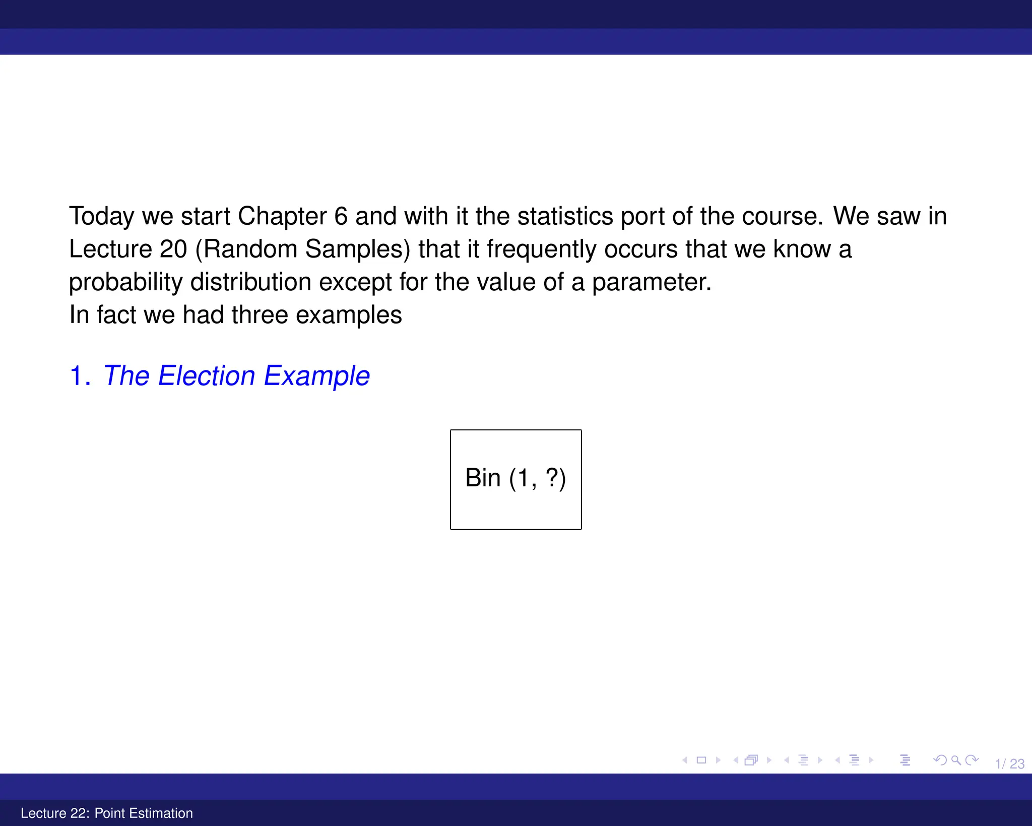
1. The Election Example
Bin (1, ?)
Lecture 22: Point Estimation

3. 2/ 23
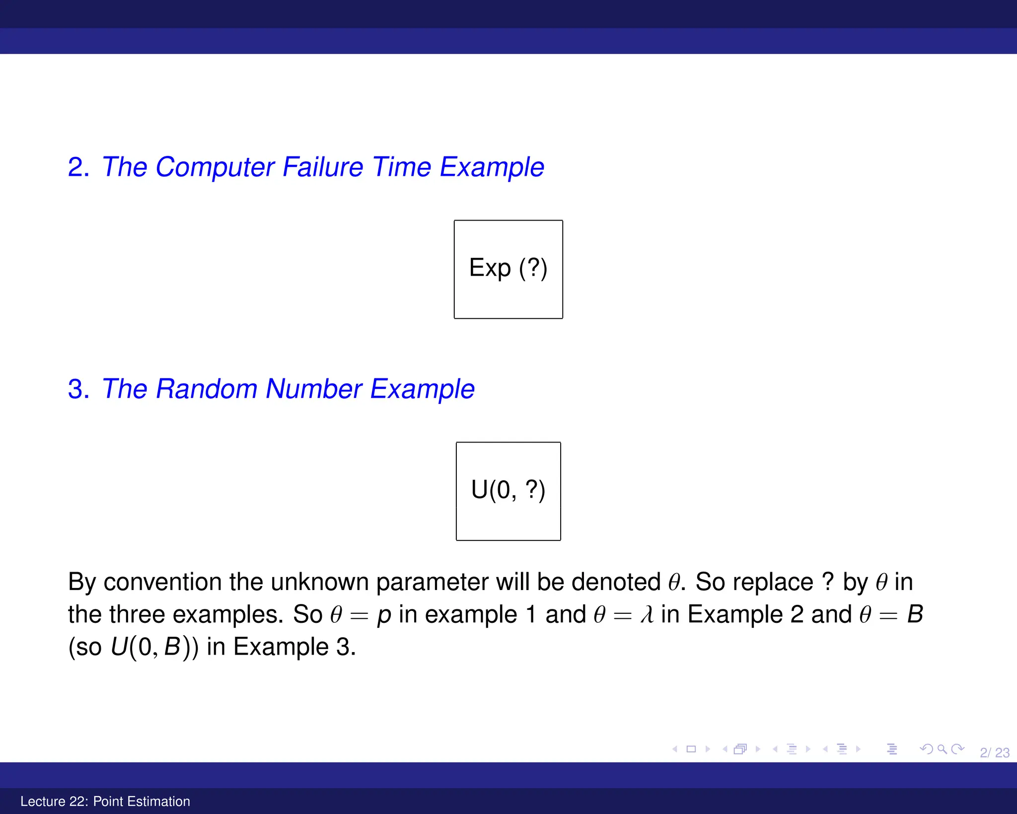
2. The Computer Failure Time Example
Exp (?)
3. The Random Number Example
U(0, ?)
By convention the unknown parameter will be denoted θ. So replace ? by θ in
the three examples. So θ = p in example 1 and θ = λ in Example 2 and θ = B
(so U(0, B)) in Example 3.
Lecture 22: Point Estimation

4. 3/ 23
If the population X is discrete we will write its pmf as pX (x, θ) to emphasize that
it depends on the unknown parameter θ and if X is continuous we will write its
pdf as fX (x, θ) again to emphasize the dependence on θ.
Important Remark
θ is a fixed number, it is just that we don’t know it. But we are allowed to make
calculations with a number we don’t know, that is the first thing we learn to do in
high-school algebra, compute with “the unknown x”.
Lecture 22: Point Estimation

5. 4/ 23
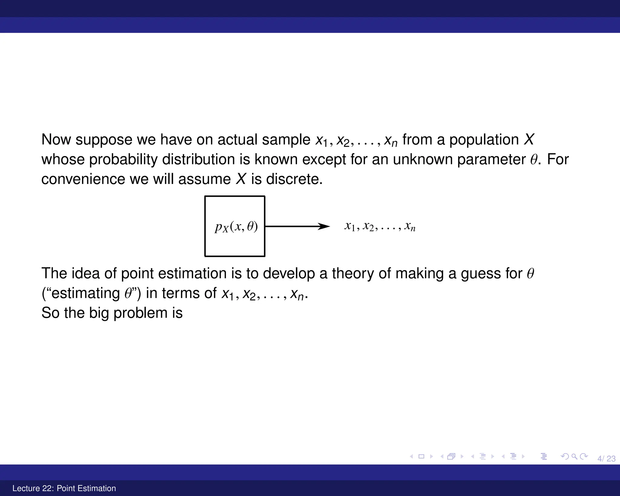
Now suppose we have on actual sample x1, x2, . . . , xn from a population X
whose probability distribution is known except for an unknown parameter θ. For
convenience we will assume X is discrete.
The idea of point estimation is to develop a theory of making a guess for θ
(“estimating θ”) in terms of x1, x2, . . . , xn.
So the big problem is
Lecture 22: Point Estimation

6. 5/ 23
The Main Problem (Vague Version)
What function h(x1, x2, . . . , xn) of the items x1, x2, . . . , xn in the sample should we
pick to estimate θ ?
Definition
Any function w = h(x1, x2, . . . , xn) we choose to estimate θ will be called an
estimator for θ.
As first one might ask -
find h so that for every sample
x1, x2, . . . , xn we have
h(x1, x2, . . . , xn) = θ.









(∗)
This is hopelessly naive. Let’s try something else
Lecture 22: Point Estimation

7. 6/ 23
The Main Problem (some what more precise)
Give quantitative criteria to decide whether one estimator w1 = h1(x1, x2, . . . , xn)
for θ is better than another estimator w2 = h2(x1, x2, . . . , xn) for θ.
The above version, though better, is not precise enough.
In order to pose the problem correctly we need to consider random samples
from X, in ofter words go back before an actual sample is taken or “go random”.
Lecture 22: Point Estimation

8. 7/ 23
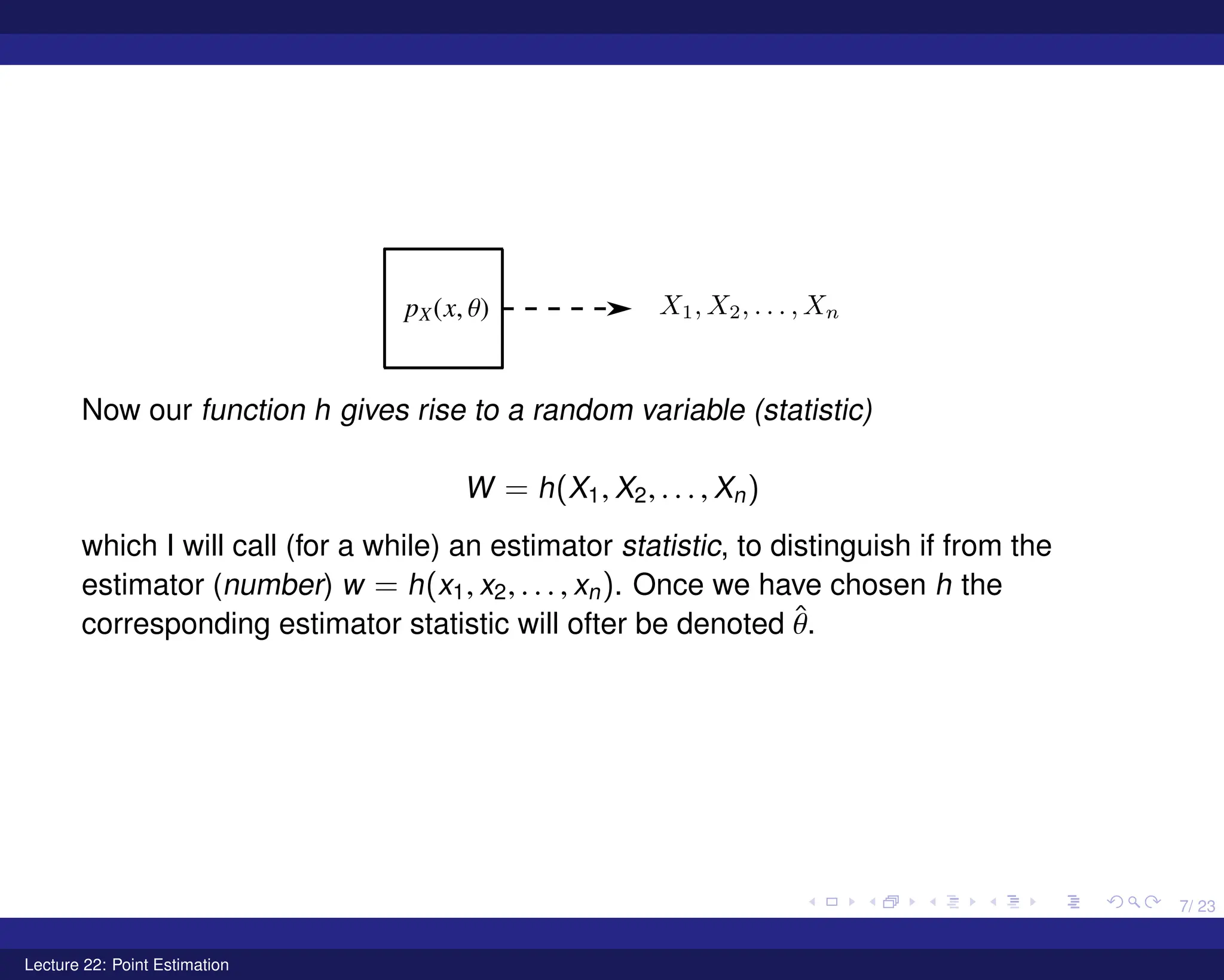
Now our function h gives rise to a random variable (statistic)
W = h(X1, X2, . . . , Xn)
which I will call (for a while) an estimator statistic, to distinguish if from the
estimator (number) w = h(x1, x2, . . . , xn). Once we have chosen h the
corresponding estimator statistic will ofter be denoted θ̂.
Lecture 22: Point Estimation

9. 8/ 23
Main Problem (third version)
Find an estimator h(x1, x2, . . . , xn) so that
P(h(X1, X2, . . . , Xn) = θ) (∗∗)
is maximized
This is what we want but it is too hard to implement - after all we don’t know θ.
Important Remark
We have made a huge gain by “going random”. The statement “maximize
P(h(x1, x2, . . . , xn) = θ)” does not make sense because h(x1, x2, . . . , xn) is a
fixed real number so either it is equal to θ or it is not equal to θ. But
P(h(X1, X2, . . . , Xn)) = θ does make sense because h(X1, X2, . . . , Xn) is a
random variable.
Now we weaken (∗∗) to something that can be achieved, in fact achieved
surprisingly easily.
Lecture 22: Point Estimation

10. 9/ 23
Unbiased Estimators Main Problem (fourth version)
Find an estimator w = h(x1, . . . , xn) so that the expected value E(W) of the
estimator statistic W = h(X1, X2, . . . , Xn) is equal to θ.
Definition
If an estimator W for an unknown parameter θ satisfies W satisfies E(W) = θ
then the estimator W is said to be unbiased.
Intuitively, requiring E(W) = θ is a good idea but we can make this move
precise. Various theorems in probability e.g Chebyshev’s inequality, tell us that if
Y is a random variable and y1, y2, . . . , yn are observed values of Y then the
numbers y1, y2, . . . , yn will tend to be near E(Y).
Applying this to our statistic W- if we take many samples of size n and compute
the value of our estimator h on each one to obtain many observed values of W
then the resulting numbers will be near E(W). But we want these to be near θ.
So we want
E(W) = θ
Lecture 22: Point Estimation

11. 10/ 23
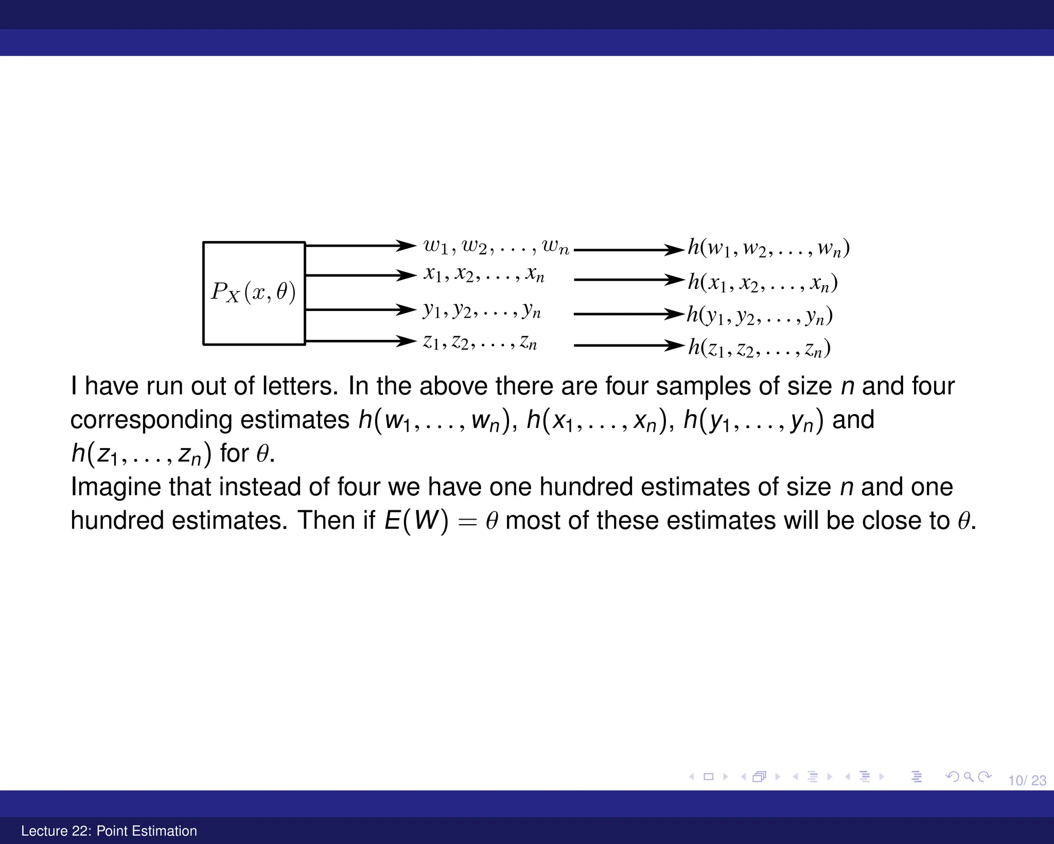
I have run out of letters. In the above there are four samples of size n and four
corresponding estimates h(w1, . . . , wn), h(x1, . . . , xn), h(y1, . . . , yn) and
h(z1, . . . , zn) for θ.
Imagine that instead of four we have one hundred estimates of size n and one
hundred estimates. Then if E(W) = θ most of these estimates will be close to θ.
Lecture 22: Point Estimation

12. 11/ 23
Examples of Unbiased Estimators
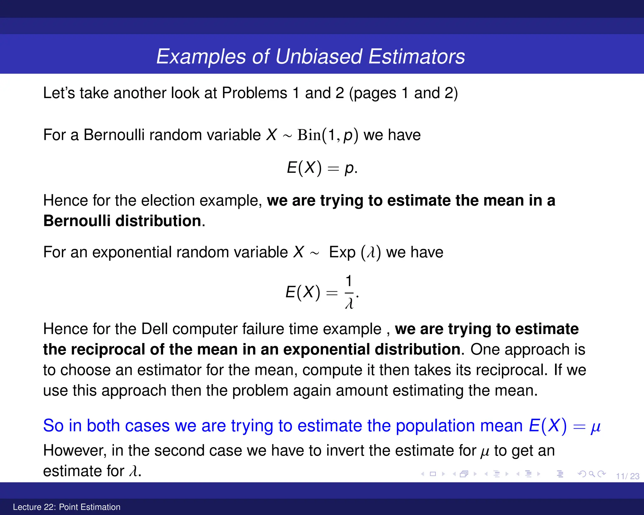
Let’s take another look at Problems 1 and 2 (pages 1 and 2)
For a Bernoulli random variable X ∼ Bin(1, p) we have
E(X) = p.
Hence for the election example, we are trying to estimate the mean in a
Bernoulli distribution.
For an exponential random variable X ∼ Exp (λ) we have
E(X) =
1
λ
.
Hence for the Dell computer failure time example , we are trying to estimate
the reciprocal of the mean in an exponential distribution. One approach is
to choose an estimator for the mean, compute it then takes its reciprocal. If we
use this approach then the problem again amount estimating the mean.
So in both cases we are trying to estimate the population mean E(X) = µ
However, in the second case we have to invert the estimate for µ to get an
estimate for λ.
Lecture 22: Point Estimation

13. 12/ 23
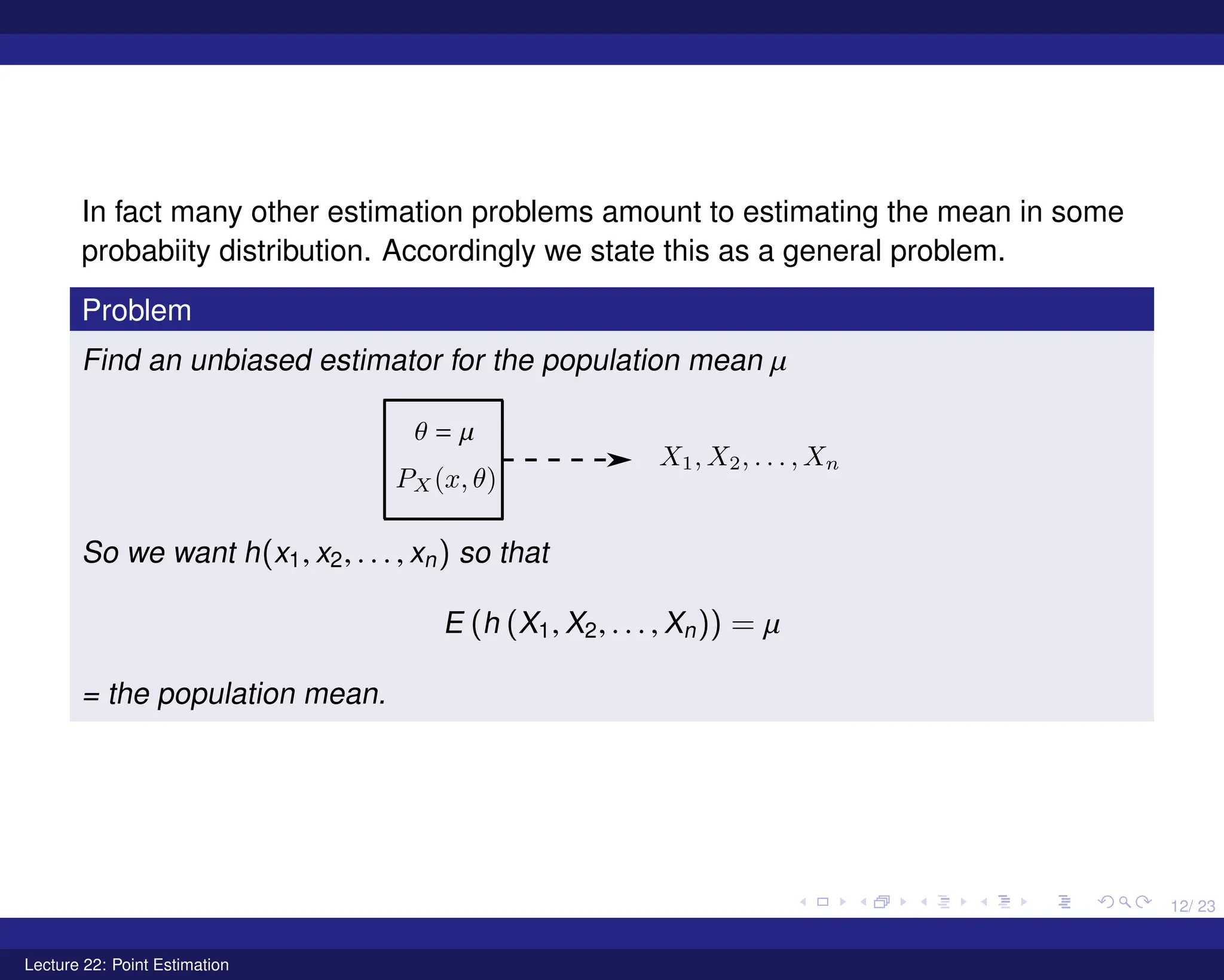
In fact many other estimation problems amount to estimating the mean in some
probabiity distribution. Accordingly we state this as a general problem.
Problem
Find an unbiased estimator for the population mean µ
So we want h(x1, x2, . . . , xn) so that
E (h (X1, X2, . . . , Xn)) = µ
= the population mean.
Lecture 22: Point Estimation

14. 13/ 23
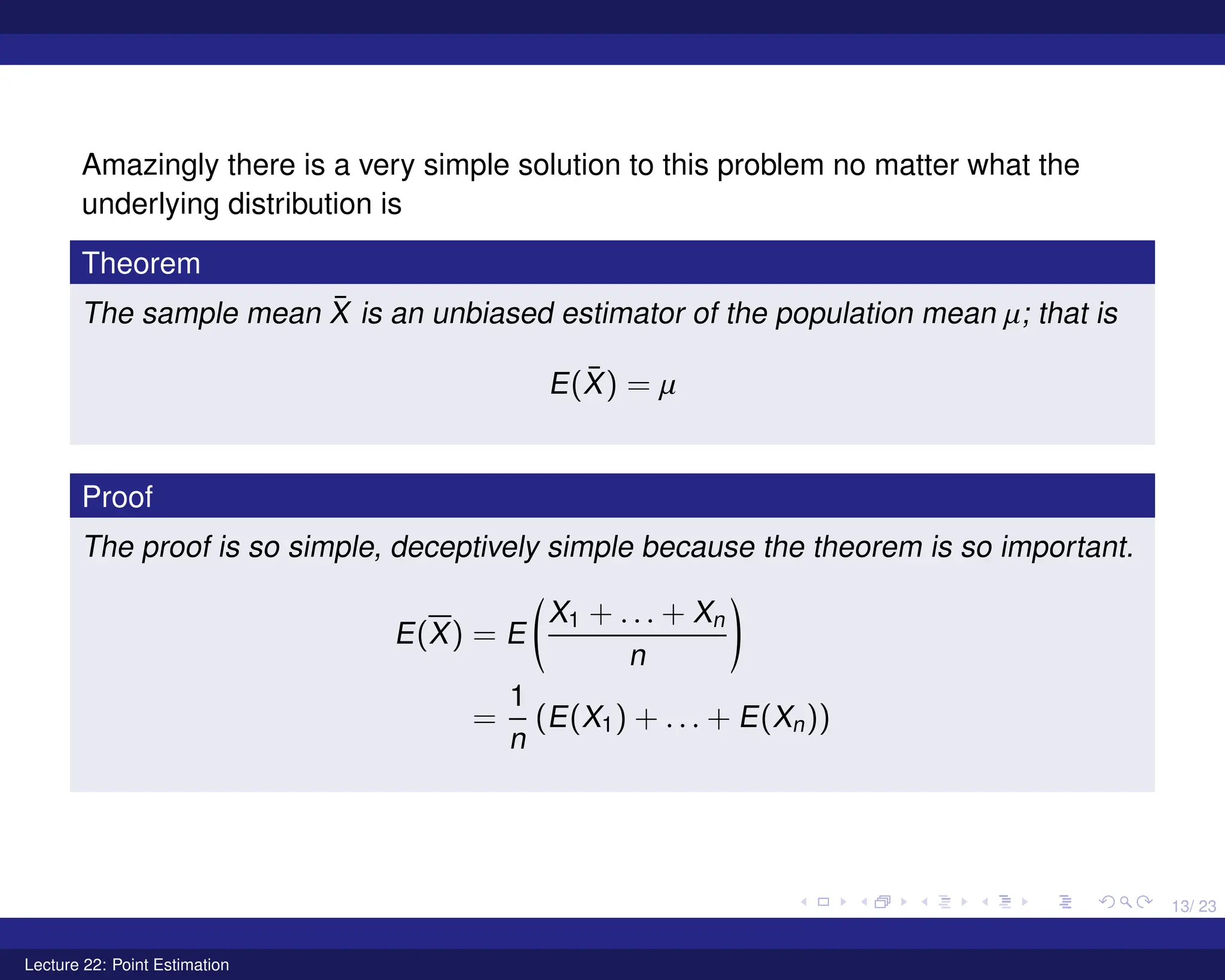
Amazingly there is a very simple solution to this problem no matter what the
underlying distribution is
Theorem
The sample mean X̄ is an unbiased estimator of the population mean µ; that is
E(X̄) = µ
Proof
The proof is so simple, deceptively simple because the theorem is so important.
E(X) = E
X1 + . . . + Xn
n
!
=
1
n
(E(X1) + . . . + E(Xn))
Lecture 22: Point Estimation

15. 14/ 23
Proof (Cont.)
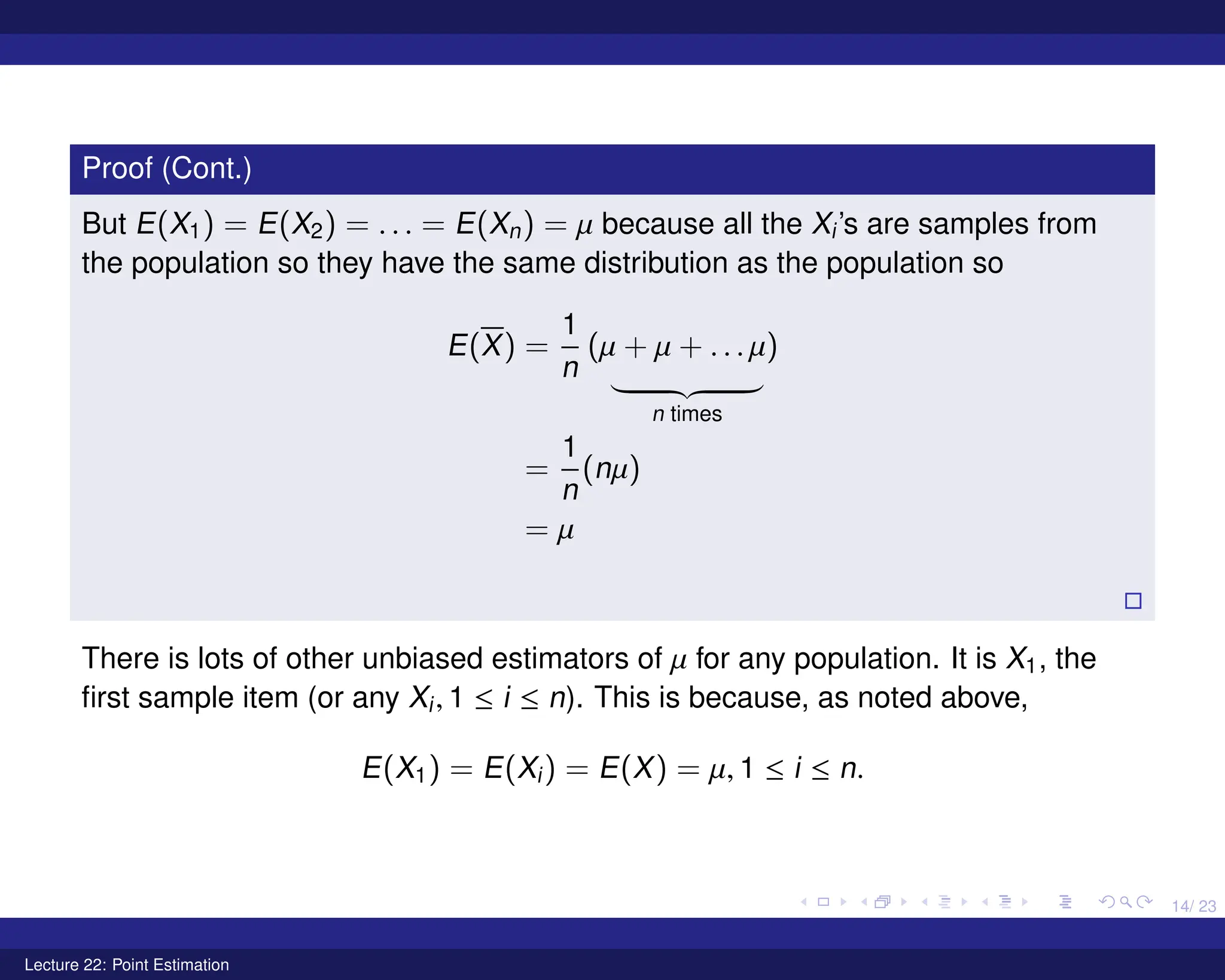
But E(X1) = E(X2) = . . . = E(Xn) = µ because all the Xi’s are samples from
the population so they have the same distribution as the population so
E(X) =
1
n
(µ + µ + . . . µ)
| {z }
n times
=
1
n
(nµ)
= µ
There is lots of other unbiased estimators of µ for any population. It is X1, the
first sample item (or any Xi, 1 ≤ i ≤ n). This is because, as noted above,
E(X1) = E(Xi) = E(X) = µ, 1 ≤ i ≤ n.
Lecture 22: Point Estimation

16. 15/ 23
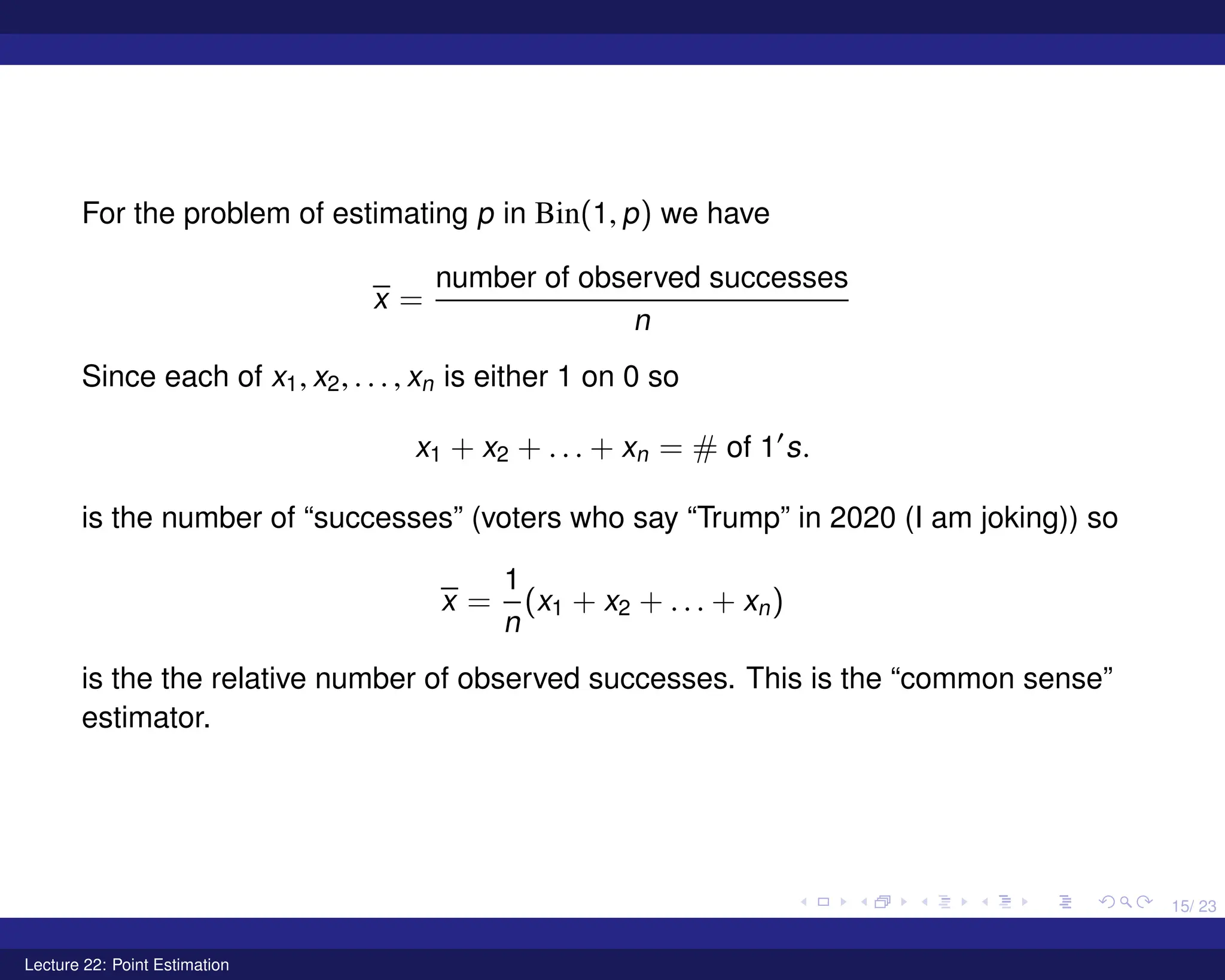
For the problem of estimating p in Bin(1, p) we have
x =
number of observed successes
n
Since each of x1, x2, . . . , xn is either 1 on 0 so
x1 + x2 + . . . + xn = # of 10
s.
is the number of “successes” (voters who say “Trump” in 2020 (I am joking)) so
x =
1
n
(x1 + x2 + . . . + xn)
is the the relative number of observed successes. This is the “common sense”
estimator.
Lecture 22: Point Estimation

17. 16/ 23
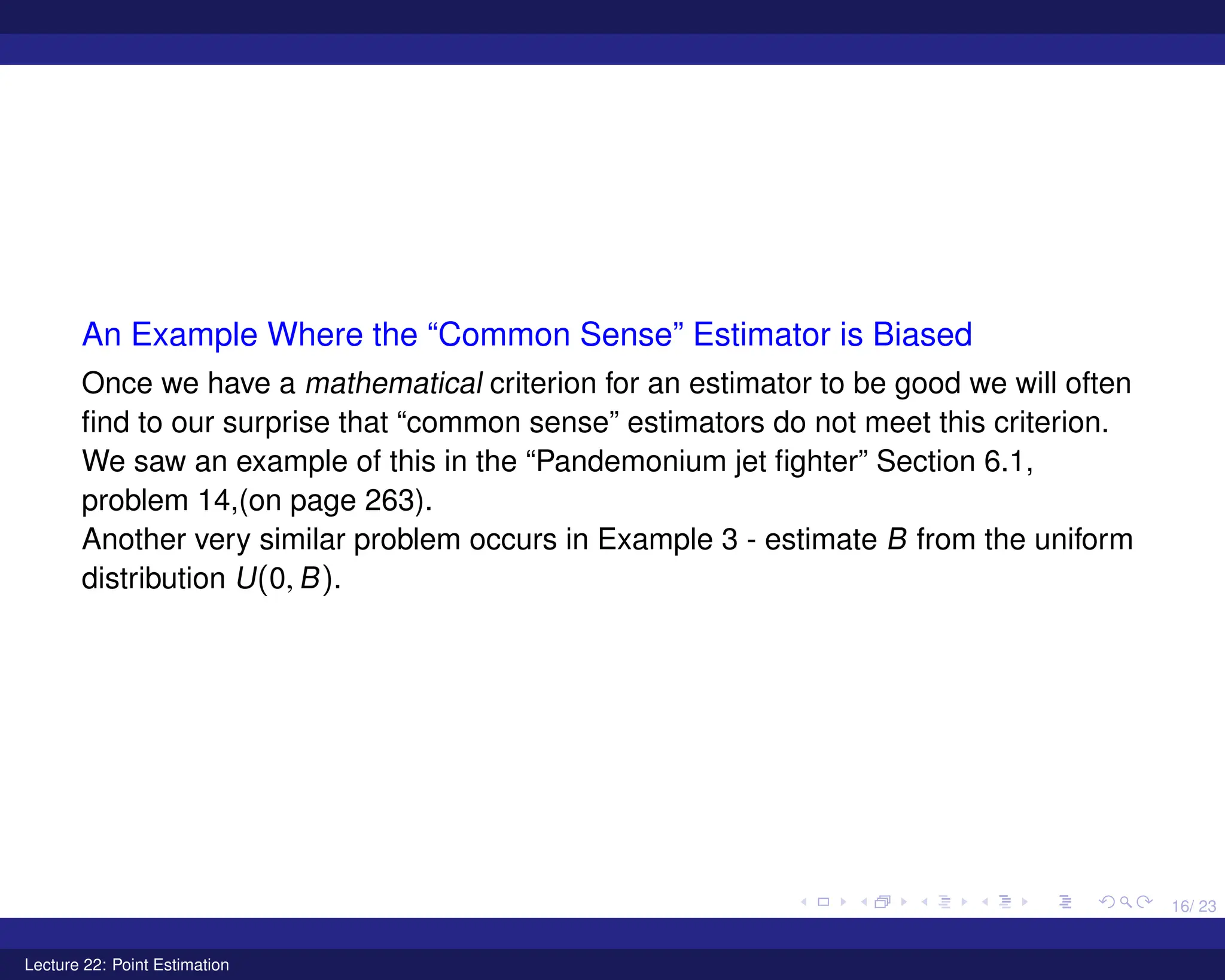
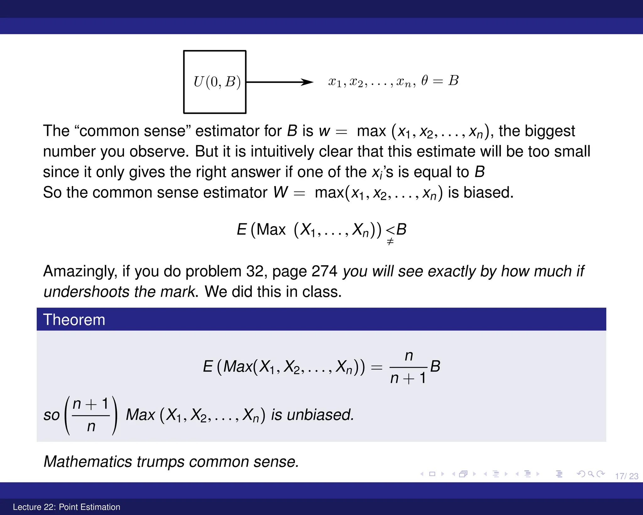
An Example Where the “Common Sense” Estimator is Biased
Once we have a mathematical criterion for an estimator to be good we will often
find to our surprise that “common sense” estimators do not meet this criterion.
We saw an example of this in the “Pandemonium jet fighter” Section 6.1,
problem 14,(on page 263).
Another very similar problem occurs in Example 3 - estimate B from the uniform
distribution U(0, B).
Lecture 22: Point Estimation

18. 17/ 23
The “common sense” estimator for B is w = max (x1, x2, . . . , xn), the biggest
number you observe. But it is intuitively clear that this estimate will be too small
since it only gives the right answer if one of the xi’s is equal to B
So the common sense estimator W = max(x1, x2, . . . , xn) is biased.
E (Max (X1, . . . , Xn))
,
B
Amazingly, if you do problem 32, page 274 you will see exactly by how much if
undershoots the mark. We did this in class.
Theorem
E (Max(X1, X2, . . . , Xn)) =
n
n + 1
B
so
n + 1
n
!
Max (X1, X2, . . . , Xn) is unbiased.
Mathematics trumps common sense.
Lecture 22: Point Estimation

19. 18/ 23
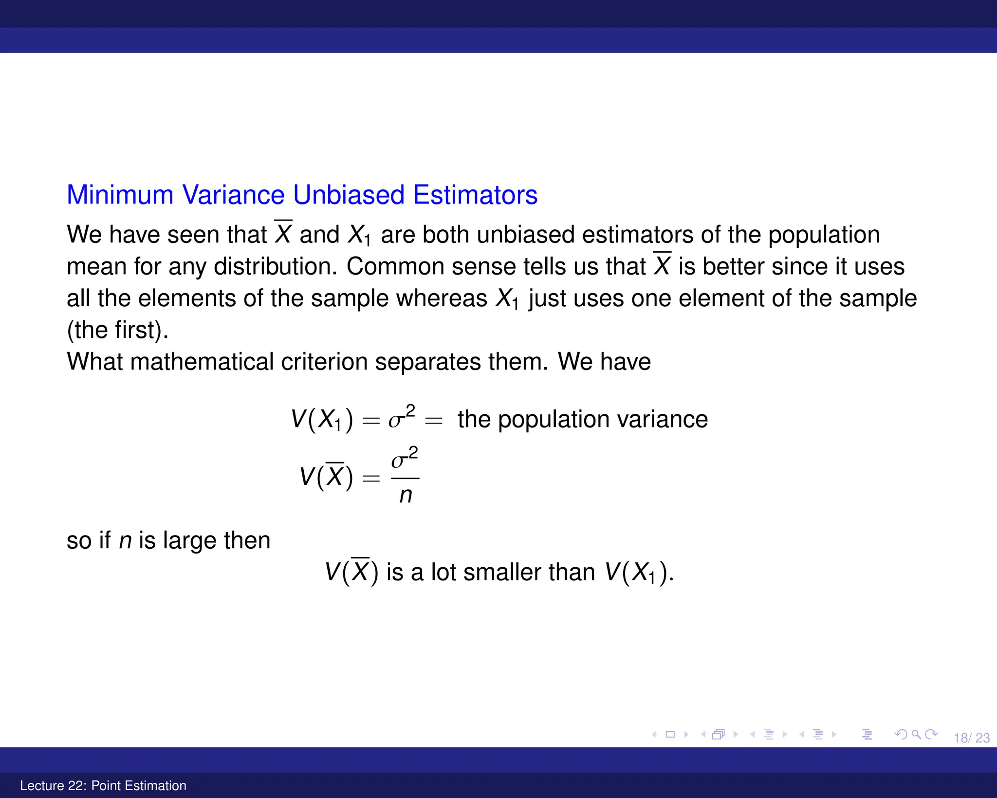
Minimum Variance Unbiased Estimators
We have seen that X and X1 are both unbiased estimators of the population
mean for any distribution. Common sense tells us that X is better since it uses
all the elements of the sample whereas X1 just uses one element of the sample
(the first).
What mathematical criterion separates them. We have
V(X1) = σ2
= the population variance
V(X) =
σ2
n
so if n is large then
V(X) is a lot smaller than V(X1).
Lecture 22: Point Estimation

20. 19/ 23
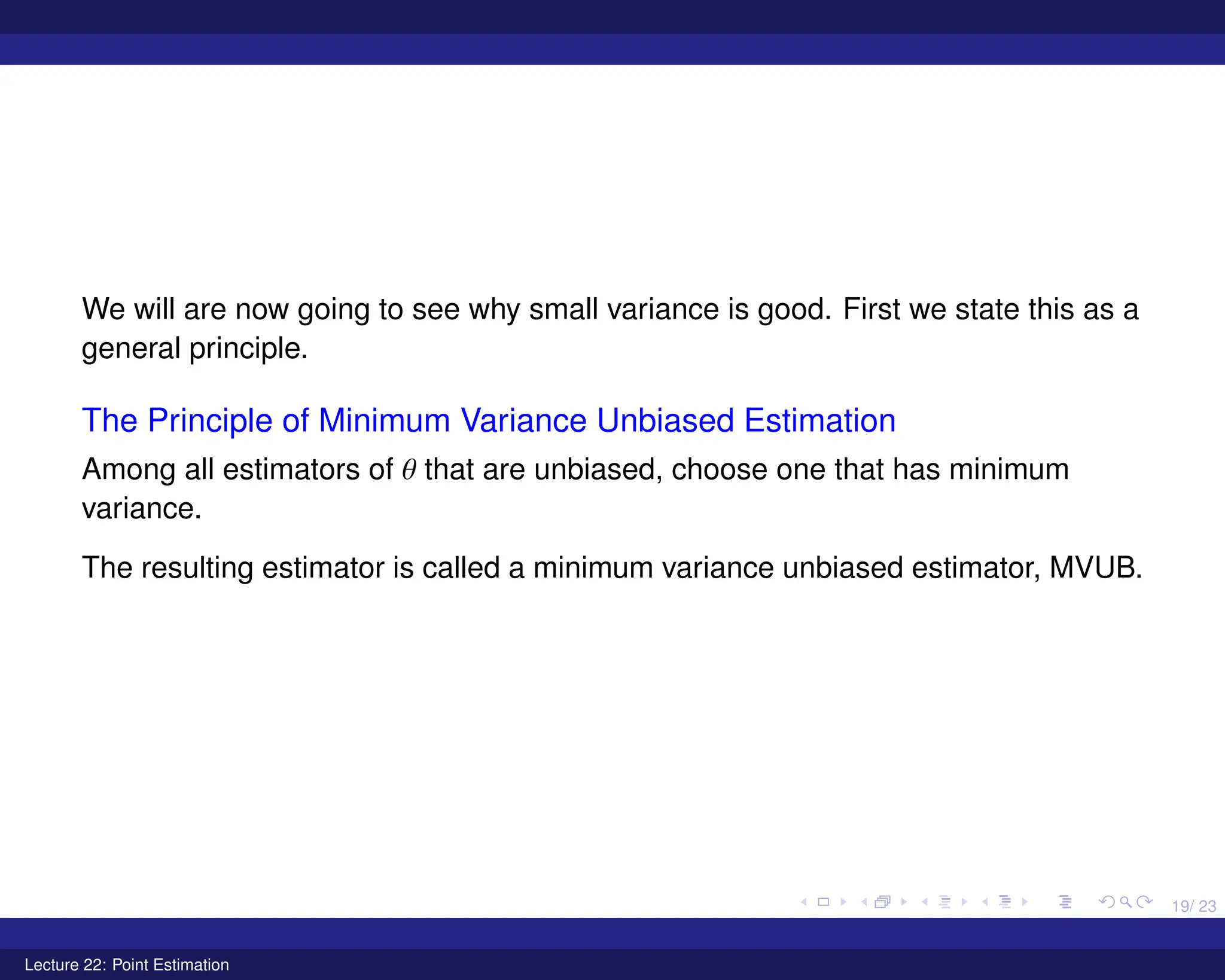
We will are now going to see why small variance is good. First we state this as a
general principle.
The Principle of Minimum Variance Unbiased Estimation
Among all estimators of θ that are unbiased, choose one that has minimum
variance.
The resulting estimator is called a minimum variance unbiased estimator, MVUB.
Lecture 22: Point Estimation

21. 20/ 23
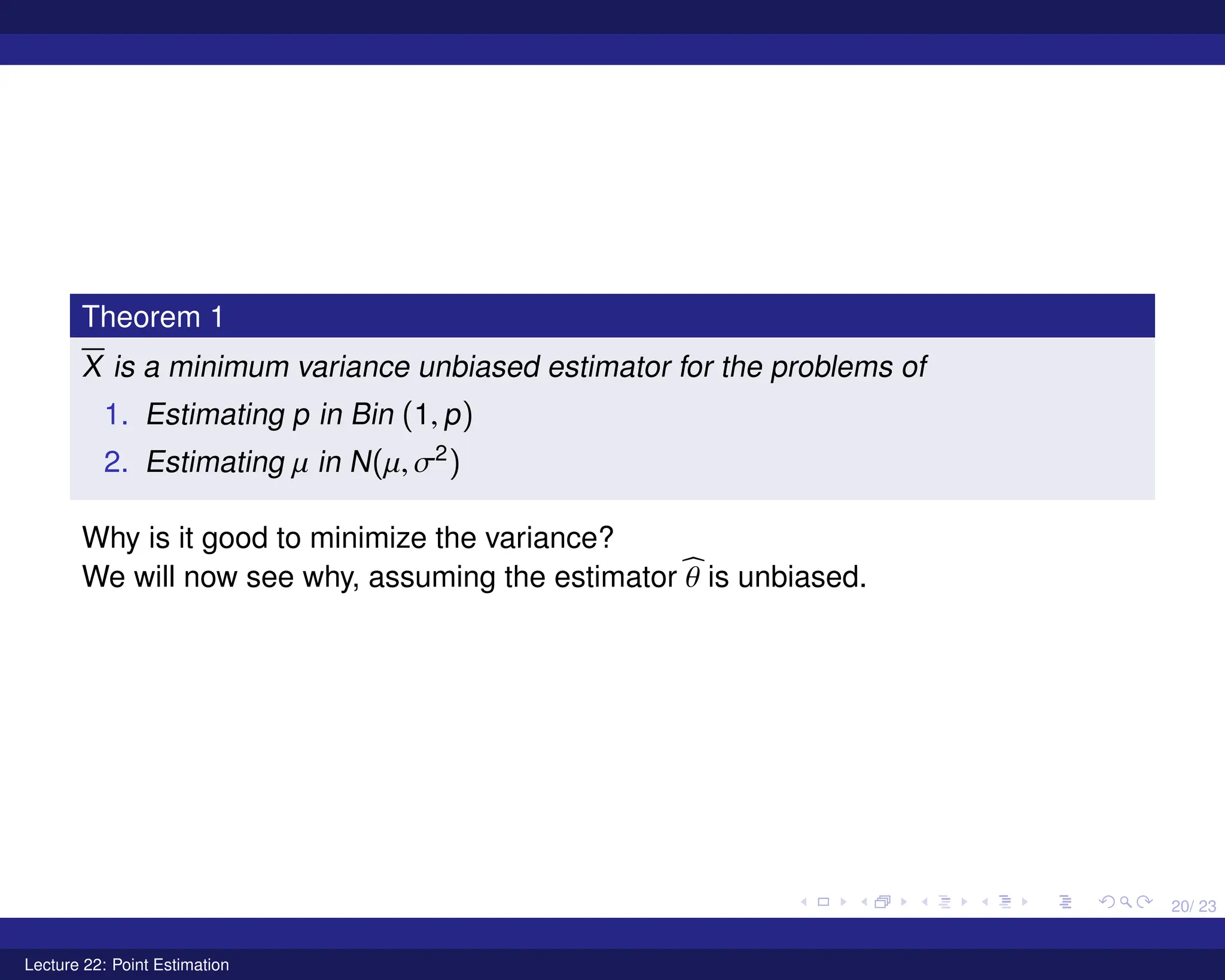
Theorem 1
X is a minimum variance unbiased estimator for the problems of
1. Estimating p in Bin (1, p)
2. Estimating µ in N(µ, σ2
)
Why is it good to minimize the variance?
We will now see why, assuming the estimator b
θ is unbiased.
Lecture 22: Point Estimation

22. 21/ 23
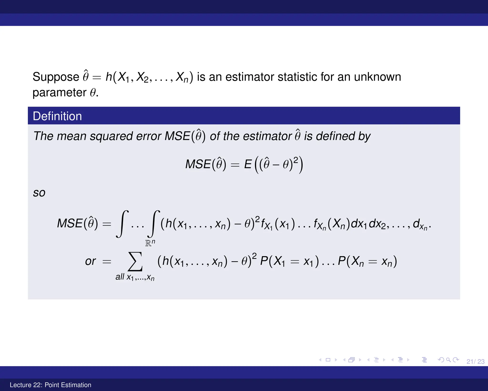
Suppose θ̂ = h(X1, X2, . . . , Xn) is an estimator statistic for an unknown
parameter θ.
Definition
The mean squared error MSE(θ̂) of the estimator θ̂ is defined by
MSE(θ̂) = E
(θ̂ − θ)2
so
MSE(θ̂) =
Z
. . .
Z
Rn
(h(x1, . . . , xn) − θ)2
fX1 (x1) . . . fXn (Xn)dx1dx2, . . . , dxn .
or =
X
all x1,...,xn
(h(x1, . . . , xn) − θ)2
P(X1 = x1) . . . P(Xn = xn)
Lecture 22: Point Estimation

23. 22/ 23
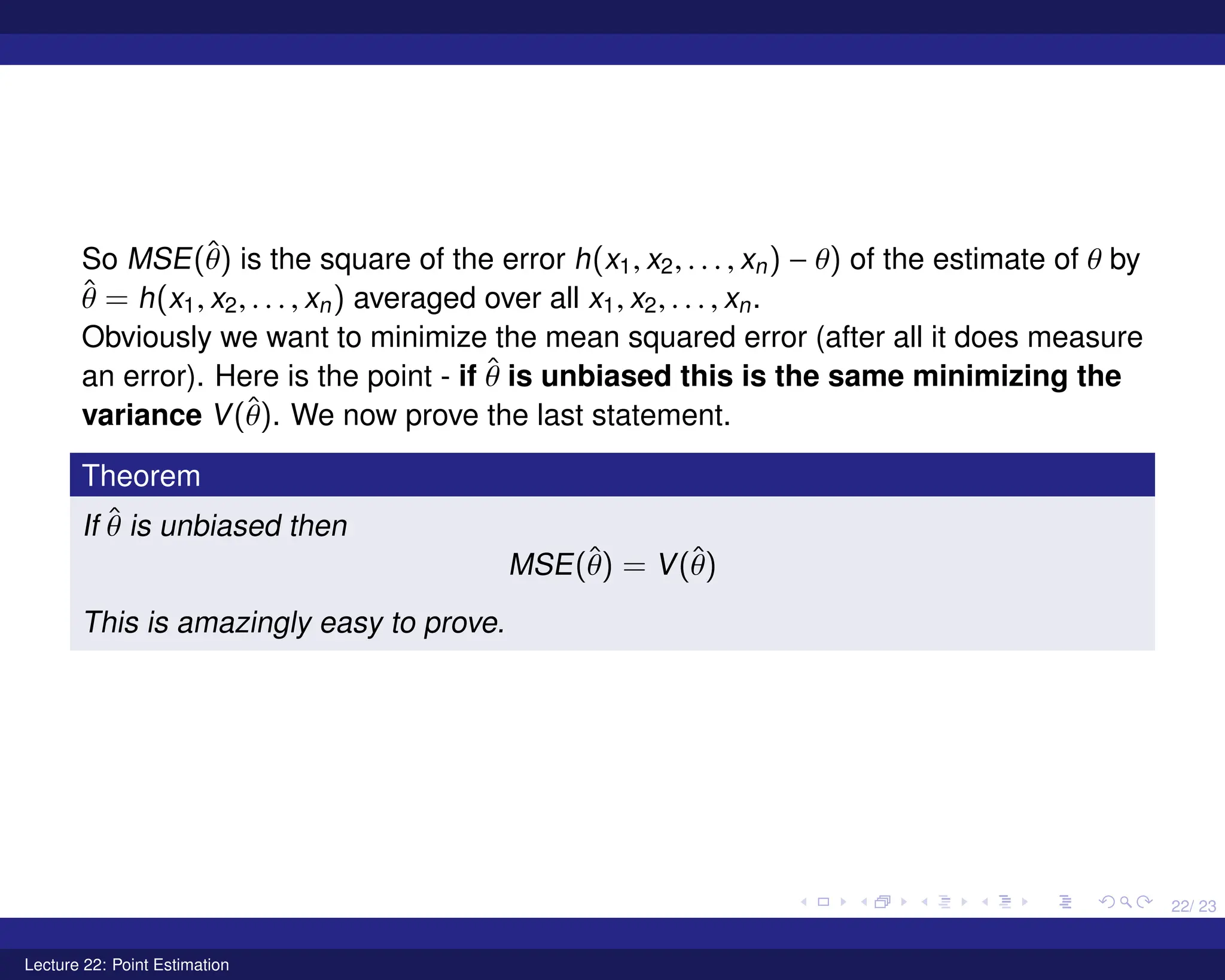
So MSE(θ̂) is the square of the error h(x1, x2, . . . , xn) − θ) of the estimate of θ by
θ̂ = h(x1, x2, . . . , xn) averaged over all x1, x2, . . . , xn.
Obviously we want to minimize the mean squared error (after all it does measure
an error). Here is the point - if θ̂ is unbiased this is the same minimizing the
variance V(θ̂). We now prove the last statement.
Theorem
If θ̂ is unbiased then
MSE(θ̂) = V(θ̂)
This is amazingly easy to prove.
Lecture 22: Point Estimation

24. 23/ 23
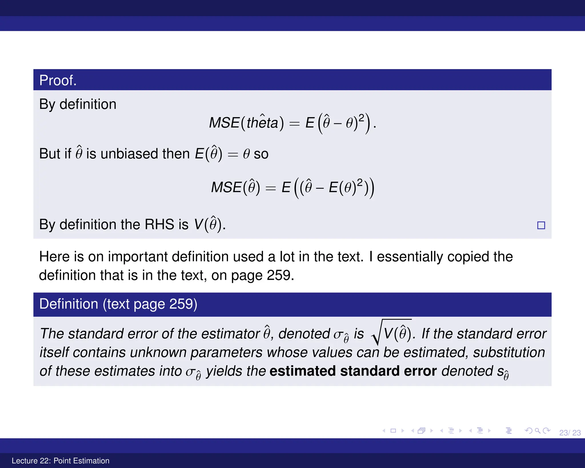
Proof.
By definition
MSE( ˆ
theta) = E
θ̂ − θ)2
.
But if θ̂ is unbiased then E(θ̂) = θ so
MSE(θ̂) = E
(θ̂ − E(θ)2
)
By definition the RHS is V(θ̂).
Here is on important definition used a lot in the text. I essentially copied the
definition that is in the text, on page 259.
Definition (text page 259)
The standard error of the estimator θ̂, denoted σθ̂ is
q
V(θ̂). If the standard error
itself contains unknown parameters whose values can be estimated, substitution
of these estimates into σθ̂ yields the estimated standard error denoted sθ̂
Lecture 22: Point Estimation