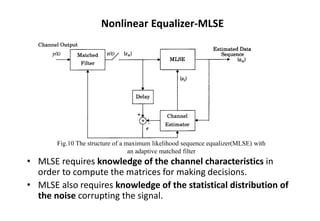
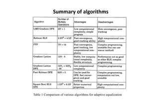
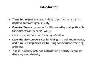
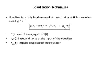
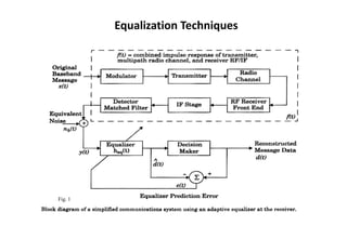
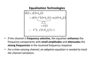
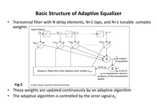
The document discusses various techniques for equalization and adaptive equalization algorithms. It describes three main techniques used for improving receiver signal quality: equalization, diversity, and channel coding. Equalization compensates for interference created by multipath channels, while diversity reduces fading. Channel coding adds redundant bits to transmitted messages. The document then covers linear and nonlinear equalization techniques, including transversal filters, decision feedback equalization, and maximum likelihood sequence estimation. It also discusses factors that influence the choice of equalization structure and algorithm, such as channel characteristics and computational complexity. Finally, it provides a brief overview of common adaptive equalization algorithms like zero forcing, LMS, and RLS.

1. Equalization
• Introduction
• Equalization Techniques
• Algorithms for Adaptive Equalization

2. Introduction
• Three techniques are used independently or in tandem to
improve receiver signal quality
• Equalization compensates for ISI created by multipath with
time dispersive channels (W>BC)
• Linear equalization, nonlinear equalization
• Diversity also compensates for fading channel impairments,
and is usually implemented by using two or more receiving
antennas
• Spatial diversity, antenna polarization diversity, frequency
diversity, time diversity

3. Introduction
• The former (Equalization) counters the effects of time
dispersion (ISI), while the latter (Diversity) reduces the depth
and duration of the fades experienced by a receiver in a flat
fading (narrowband) channel
• Channel Coding improves mobile communication link
performance by adding redundant data bits in the transmitted
message
• Channel coding is used by the Rx to detect or correct some (or
all) of the errors introduced by the channel (Post detection
technique)
• Block codes and convolution codes are mostly used.

4. Equalization Techniques
• The term equalization can be used to describe any signal
processing operation that minimizes ISI
• Two operation modes for an adaptive equalizer
: training and tracking
• Three factors affect the time spanning over which an equalizer
converges: equalizer algorithm, equalizer structure and time
rate of change of the multipath radio channel
• TDMA wireless systems are particularly well suited for
equalizers

5. Equalization Techniques
• Equalizer is usually implemented at baseband or at IF in a receiver
(see Fig. 1)
• f*(t): complex conjugate of f(t)
• nb(t): baseband noise at the input of the equalizer
• heq(t): impulse response of the equalizer
)
t
(
b
n
)
t
(
f
)
t
(
x
)
t
(
y +

= 

6. Equalization Techniques
Fig. 1

7. Equalization Technologies
• If the channel is frequency selective, the equalizer enhances the
frequency components with small amplitudes and attenuates the
strong frequencies in the received frequency response
• For a time-varying channel, an adaptive equalizer is needed to track
the channel variations .
( ) ( ) ( )
( ) ( ) ( ) ( ) ( )
( )
( ) ( ) 1
ˆ
=

−

=

+


=

=


f
H
f
F
t
δ
t
h
t
m
t
h
t
f
t
x
t
h
t
y
t
d
eq
eq
b
eq
eq

8. Basic Structure of Adaptive Equalizer
• Transversal filter with N delay elements, N+1 taps, and N+1 tunable complex
weights
Fig-2
• These weights are updated continuously by an adaptive algorithm
• The adaptive algorithm is controlled by the error signal ek

9. Equalization Techniques
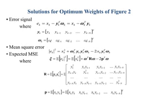
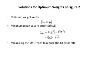
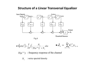
• Classical equalization theory : using training sequence to minimize the
cost function
• Recent techniques for adaptive algorithm : blind algorithms
• Constant Modulus Algorithm (CMA, used for constant envelope
modulation)
• Spectral Coherence Restoral Algorithm (SCORE, exploits spectral
redundancy or cyclostationarity in the Tx signal)
E[e(k) e*(k)]

10. Solutions for Optimum Weights of Figure 2
• Error signal
where
• Mean square error
• Expected MSE
where
k
T
k
k
k
T
k
k
k x
x
e y
y 
 −
=
−
=
 T
N
k
k
k
k
k y
....
y
y
y −
−
−
= 2
1
y
 T
N
k
k
k
k
k ω
....
ω
ω
ω −
−
−
= 2
1

k
T
k
k
k
T
k
k
T
k
k
k x
x
e 

 y
y
y 2
2
2
−
+
=
    


 T
T
k
k x
e p
R 2
2
2
−
+
=
= E
E
 












=
=
−
−
−
−
−
−
−
−
−
−
−
−
−
−
−
2
1
2
1
2
1
2
1
1
2
1
2
N
k
N
k
k
N
k
k
k
N
k
k
N
k
k
N
k
k
k
k
k
k
k
k
k
k
k
*
k
k
y
....
y
y
y
y
....
y
y
y
y
y
y
....
....
....
....
....
y
y
y
y
y
....
y
y
y
y
y
E
E y
y
R
   T
N
k
k
k
k
k
k
k
k
k
k y
x
y
x
y
x
y
x
y
x −
−
−
=
= ....
2
1
E
E
p

11. Solutions for Optimum Weights of Figure 2
• Optimum weight vector
• Minimum mean square error (MMSE)
• Minimizing the MSE tends to reduce the bit error rate
p
R 1
ˆ −
=
ω
 −
= 2
min E
ξ 
 p
R
p 1
T −
 −
= 2
E 
 ω̂
Τ
p

12. Equalization Techniques
• Two general categories - linear and nonlinear equalization (see
Fig. 3)
• In Fig. 1, if d(t) is not the feedback path to adapt the equalizer,
the equalization is linear
• In Fig. 1, if d(t) is fed back to change the subsequent outputs of
the equalizer, the equalization is nonlinear

13. Equalization Techniques
Fig.3 Classification of equalizers

14. Equalizer Techniques
Linear transversal equalizer (LTE, made up of tapped delay lines as
shown in Fig.4)
Fig.4 Basic linear transversal equalizer structure
•Finite impulse response (FIR) filter (see Fig.5)
•Infinite impulse response (IIR) filter (see Fig.5)

15. Equalizer Techniques
Fig.5 Tapped delay line filter with both feedforward and feedback taps

16. Structure of a Linear Transversal Equalizer
n
k
N
N
n
*
n
k y
C
d
2
1
−
−
=

=
• ˆ
  




d
N
e
N
T
e(n) T
T
o
j
o
−
+
=
• 2
t
2
)
(
F
2
E
)
e
(
F ω
t
j
: frequency response of the channel
o
N : noise spectral density
Fig 6

17. Structure of a Lattice Equalizer
Fig.7 The structure of a Lattice Equalizer

18. Characteristics of Lattice Filter
• Advantages
➢Numerical stability
➢Faster convergence
➢Unique structure allows the dynamic assignment of the most
effective length.
• Disadvantages
➢The structure is more complicated

19. Nonlinear Equalization
• Used in applications where the channel distrotion is too severe
• Three effective methods
➢Decision Feedback Equalization (DFE)
➢Maximum Likelihood Symbol Detection
➢Maximum Likelihood Sequence Estimator (MLSE)

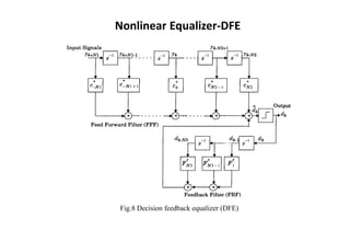
20. Nonlinear Equalization--DFE
• Basic idea : once an information symbol has been detected and
decided upon, the ISI that it induces on future symbols can be
estimated and subtracted out before detection of subsequent symbols
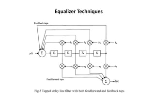
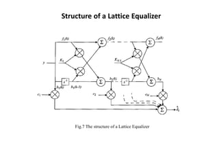
• Can be realized in either the direct transversal form (see Fig.8) or as a
lattice filter

 =
−
−
−
=
+
=
3
2
1
N
1
i
i
k
i
n
k
N
N
n
*
n
k d
F
y
C
d̂
  }
d
]
N
)
e
(
N
[
ln
2
T
{
exp
e(n) T
T o
2
T
j
o
min
2





−
+
=
F
E

21. Nonlinear Equalizer-DFE
Fig.8 Decision feedback equalizer (DFE)

22. Nonlinear Equalization--DFE
• Predictive DFE
• Consists of an FFF(Feed forward Filter) and an FBF(Feed back Filter),
the latter is called a noise predictor ( see Fig.9 )
• Predictive DFE performs as well as conventional DFE, as the limit in the
number of taps in FFF and the FBF approach infinity
• The FBF in predictive DFE can also be realized as a lattice structure .
• The RLS (recursive least squares) algorithm can be used to yield fast
convergence

23. Nonlinear Equalizer-DFE
Fig.9 Predictive decision feedback equalizer

24. Nonlinear Equalization--MLSE
• MLSE tests all possible data sequences (rather than decoding each
received symbol by itself ), and chooses the data sequence with the
maximum probability as the output.
• Usually has a large computational requirement
• First proposed by Forney using a basic MLSE estimator structure and
implementing it with the Viterbi algorithm
• The block diagram of MLSE receiver (see Fig.10 )

25. Nonlinear Equalizer-MLSE
• MLSE requires knowledge of the channel characteristics in
order to compute the matrices for making decisions.
• MLSE also requires knowledge of the statistical distribution of
the noise corrupting the signal.
Fig.10 The structure of a maximum likelihood sequence equalizer(MLSE) with
an adaptive matched filter

26. Algorithm for Adaptive Equalization
• Performance measures for an algorithm
➢Rate of convergence
➢Mis-adjustment
➢Computational complexity
➢Numerical properties
• Factors dominate the choice of an equalization structure and its
algorithm
➢The cost of computing platform
➢The power budget
➢The radio propagation characteristics

27. Algorithm for Adaptive Equalization
• The speed of the mobile unit determines the channel fading rate and
the Doppler spread, which is related to the coherent time of the
channel directly
• The choice of algorithm, and its corresponding rate of convergence,
depends on the channel data rate and coherent time
• The number of taps used in the equalizer design depends on the
maximum expected time delay spread of the channel
• The circuit complexity and processing time increases with the number
of taps and delay elements

28. Algorithm for Adaptive Equalization
• Three classic equalizer algorithms : zero forcing (ZF), least mean
squares (LMS), and recursive least squares (RLS) algorithms
• Summary of algorithms (see Table 1)

29. Summary of algorithms
Table 1 Comparison of various algorithms for adaptive equalization