Downloaded 275 times
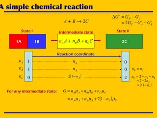
![A simple chemical reaction
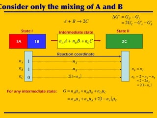
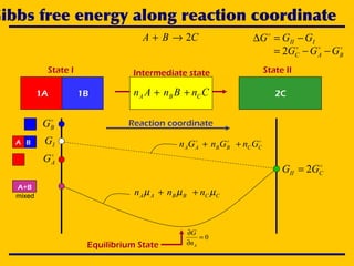
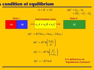
State I State II
CBA 2→+
1A 1B 2CCnBnAn CBA ++
Intermediate state
III GGG −=∆
BAC GGG −−= 2
( ) CABAAA nnn µµµ −++= 12CCBBAA nnnG µµµ ++=
Recall: iii aRTG ln+=
µ
( ) ( ) ( )( )CCABBAAAA aRTGnaRTGnaRTGnG ln12lnln +−++++=
( ) ( )[ ]CABAAACABAAA anananRTGnGnGn ln12lnln12 −+++−++=
( ) 0ln2lnln2 =−++−+=
∂
∂
CBACBA
A
aaaRTGGG
n
G
Find
minimum
along
reaction
coordinate:
G∆−
( )CBA aaaRTG ln2lnln −+=∆ ](https://image.slidesharecdn.com/lecture-17-ellingham2-101114121300-phpapp01/85/Ellingham-Diagram-Aftab-Ahmed-Laghari-6-320.jpg)
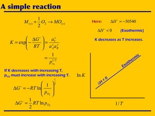
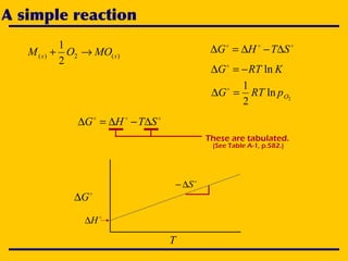
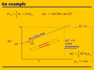
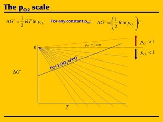
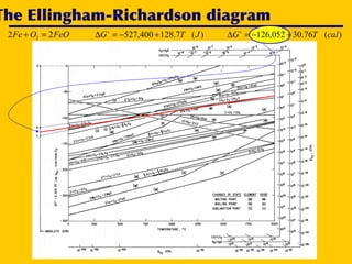
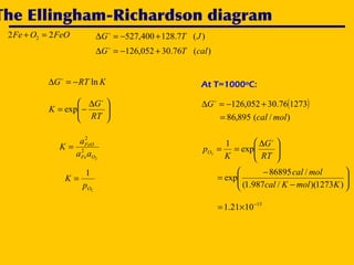
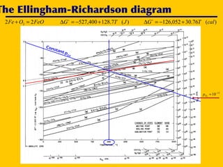
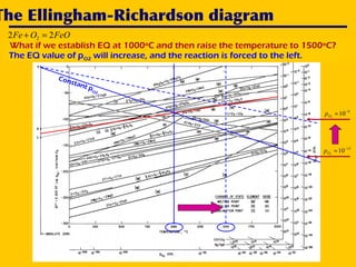

1. The document discusses thermodynamics and Ellingham diagrams for analyzing chemical reaction equilibria. It covers concepts like Gibbs free energy, equilibrium constants, and the temperature dependence of reactions. 2. An Ellingham diagram graphs the standard Gibbs free energy of formation of metal oxides as a function of temperature. This allows analyzing the stability of metals and oxides under different oxygen partial pressures and temperatures. 3. The document uses the iron-oxygen reaction to illustrate how the equilibrium oxygen partial pressure increases with temperature according to the Ellingham diagram in order to maintain equilibrium.