1
Supply Chain Management
INDE 6641
Inventory Management (II)
Economic Order Quantity (EOQ)
Dr. Narjes Sadeghiamirshahidi
Department of Mechanical and Industrial Engineering
Copyright © 2015 by Steven Nahmias and Tava Lennon Olsen. All Rights Reserved
2
Inventory Costs
 Carrying (holding) Cost: all Costs that are proportional to amount of Inventory on hand.
Carrying (holding) Cost It includes:
• Cost of Physical Space to store Items
• Taxes and Insurance
• Breakage, Spoilage, and Deterioration
• Opportunity Cost of alternative Investment
 Ordering Cost: depends on amount of Inventory that is Ordered or Produced.
Ordering Cost has two Components:
• Fixed Ordering Cost (): does not depend on size of Order
• Variable Ordering Cost (): depends on size of Order (Cost of one Unit)
 Shortage (Penalty/Stock-out) Cost: Cost of not having sufficient Stock on hand to satisfy
Customers Demand.
3
Inventory Costs – Holding Cost
Carrying (holding) Cost is based on average Inventory level
Annual Interest Rate () commonly includes four Components:
 Cost of Capital
 Taxes and Insurance
 Cost of Storage
 Breakage, Spoilage, and Deterioration
: Annual holding Cost (Dollar per Unit)
: Annual Interest Rate
: Dollar Value of one Unit of Inventory
h=𝑖𝑐
4
Inventory Costs – Holding Cost: Example
Example: Assume
• Cost of Capital= 28%
• Taxes and Insurance = 2%
• Cost of Storage = 6%
• Breakage, Spoilage, and Deterioration = 1%
1) Calculate Total Annual Interest Rate.
2) Calculate Annual holding Cost if one Item Valued at $180.
𝒊=𝟐𝟖% +𝟐%+𝟔%+𝟏%=𝟑𝟕%
1) Total Annual Interest Rate:
Solution:
2) Annual holding Cost if one Item Valued at $180:
h=𝑖𝑐 =(0.37)($180)= $66.6
= 0.37
𝒄=$𝟏𝟖𝟎
5
Inventory as a Function of Time
Holding Cost of Items for years = ()()() = ()()()
I(t
)
Time
T
0
𝐼=
1
𝑇
∫
0
𝑇
𝐼(𝑡) 𝑑𝑡=
Shaded Area
T
Average Inventory Level ():
6
Inventory as a Function of Time – Example
Example: A Company wants to keep 300 of Product A for 5 Years.
Suppose the Annual Interest Rate is 37% & Dollar Value of one Unit of Inventory of
Product A is $180. Calculate Average Inventory Level & Holding Cost of Items for 5 Years.
I(t)
Time
5
300
0
Holding Cost of items for 5 years = ()()() =)()() = $99,900
Average Inventory Level ():
Given Information:
= 0.37
= 5 years
𝒄=$𝟏𝟖𝟎
Desired Product Quantity = 300
=(0.37)($180)=$66.6
Annual holding Cost:
Solution:
7
Inventory as a Function of Time
Average Inventory Level () during Period ():
2
1
2 1
1
( )
( )
t
t
I I t dt
t t

 
Area under the Curve divided by
Average Inventory Level ():
8
Inventory Costs – Ordering Cost
Ordering Cost : depends on amount of Inventory that is Ordered or Produced
Ordering Cost has two Components:
 Fixed Ordering Cost ()*: does not depend on size of Order
 Variable Ordering Cost (): depends on size of Order (Cost of one Unit)
𝐶 ( 𝑥)={ 0 𝑖𝑓 𝑥=0
𝐾 +𝑐𝑥 𝑖𝑓 𝑥 >0
Total Ordering Cost:
*Fixed Ordering Cost (): are activities involved in placing an Order
including:
• Administrative Costs: expenses associated with paperwork,
communication, and processing & managing orders.
• Transportation & Shipping Costs: expenses associated with
receiving ordered Items and getting them to desired Location.
• Inspection & Quality Control Costs: costs related to checking
the received Items to ensure they meet Quality &
Specification Standards.
• Handling & Storage Costs: costs associated with moving and
storing Items until they are needed for Production or Sale.
9
Inventory Costs – Ordering Cost: Example
𝐶 ( 𝑥)=
{ 0𝑖𝑓 𝑥=0
𝐾+𝑐𝑥 𝑖𝑓 𝑥>0
Total Ordering Cost:
Example: Suppose Fixed & Variable Costs of placing Order are $50 & $2 respectively.
Calculate Ordering Cost of 100 Items.
𝑲 =$𝟓𝟎
Given Information:
𝒄=$ 𝟐
Items
𝒙=𝟏𝟎𝟎>𝟎 𝑪(𝒙)=𝑲 +𝒄𝒙
Solution:
10
Inventory Costs – Shortage Cost
Shortage (Penalty/Stock-out) Cost: Cost of not having sufficient Stock on hand to
satisfy a Demand.
• Each time a Demand occurs and can not be satisfied immediately, a Cost is
incurred regardless of how long it takes to eventually satisfy the Demand.
11
Economic Order Quantity (EOQ) Model
Economic Order Quantity (EOQ) Model:
 Is the simplest and fundamental of all Inventory Models.
 Is basis for Analysis of more Complex Systems.
 Describes the important trade-off between Ordering Cost & holding Cost
 Goal of EOQ Model: to balance Ordering Cost against holding Cost to determine the Optimal
amount of Items to order
12
Economic Order Quantity (EOQ) Model
EOQ Model Assumptions:
1. Demand Rate is known & constant over Time: Demand Rate is a constant per Unit
 Unit of Time might be Days, Weeks, Months, etc.
• Note: If Unit of Time is not given, we assume that Unit of Time is Year
2. Lead Time is known & constant and entire Order is received all at once
3. Shortages are not permitted
4. Costs include:
 Fixed Ordering Cost of an Order ()
 Variable Ordering Cost ()
 holding Cost (): per Unit per Time
13
Economic Order Quantity (EOQ) Model – Notations
EOQ Model Notations:
: Annual Demand (: Demand Rate)
: Order Quantity
: Cycle Time (Time between Orders or Average Order Interval)
: Number of Orders per Period
: Lead Time
: Average Inventory Level (Inventory Level at Time )
: holding Costs per Item per Period
: Annual Interest Rate
: Dollar Value of one Unit of Inventory Item (Variable Purchasing Price)
: Fixed Ordering Cost
holding Cost: h=𝑖𝑐 Total Ordering Cost: 𝐶 ( 𝑥)=
{ 0 𝑖𝑓 𝑥=0
𝐾 +𝑐𝑥 𝑖𝑓 𝑥>0
14
Average Inventory in EOQ Model
I(t)
Time
T
Q
Shaded Area for one Cycle (T) = 𝑻𝑸/𝟐
Annual Demand =
EQO Model:
Average Inventory for one Cycle (T) = 𝐼=
𝑄
2
Annual Number of Orders = 𝑁=
𝐷
𝑄
Remember: I(t)
Time
T
𝐼=
1
𝑇
∫
0
𝑇
𝐼(𝑡)𝑑𝑡=
Shaded Area
T
Average Inventory Level ():
Average Inventory for one Cycle (T) =
Shaded Area
T
=
𝑻𝑸/𝟐
T
=𝑸/𝟐
15
Cost of EOQ Model
Total Cost = Ordering Cost + Holding Cost
𝑇𝐶(𝑄)=
𝐾𝐷
𝑄
+𝑐𝐷 +h
𝑄
2
Number of Orders × Ordering Cost
(𝐷/𝑄)×(𝐾 +𝑐𝑄)
Average Inventory () × holding Costs per item per period
(
𝑄
2
)× h
16
Cost of EOQ Model – Cont’d
𝑇𝐶(𝑄)=
𝐾𝐷
𝑄
+𝑐𝐷+h
𝑄
2
𝑑𝑇𝐶
𝑑𝑄
=−
𝐾𝐷
𝑄
2
+
h
2
=0
𝐾𝐷
𝑄
2
=
h
2
Note: If is Demand Rate per Year: 𝑄
∗
=
√2𝐾 𝜆
h
=
√2𝐾 𝜆
𝑖𝑐
𝐸𝑂𝑄=𝑄
∗
=
√2𝐾𝐷
h
=
√2𝐾𝐷
𝑖𝑐
(Economic Order Quantity)
To find Economic Order Quantity (EOQ), we should minimize Total Cost.
Take derivative
with respect to Q
Note: Unit of Demand and holding Cost must be the same.
Meaning: if Demand is Annual, then would be holding Cost of one Unit for a Year
Note: for float Values of Q, we round it up to be on safe side
17
Graphical Representation of Cost of EOQ Model
Note: Q* is Value of Q where the two Curves (i.e., Holding Costs & Ordering Costs) intersects.
At Q*: Holding Costs = Ordering Costs
2
KD Q
h
Q

(Holding Costs)
Cost
Order Quantity (Q)
Q*
Total cost
(Ordering Costs)
2
hQ
Q
KD
18
EOQ Model – Example
Example 1: A Company supplies Valves at rate of 3000 a Month. Each Valve costs $5.00. One
Order costs $2 and Annual Interest Rate is 6%. What is Economic Order Quantity? What is Total
Cost?
𝑲 =$ 𝟐
per Month  per Year
𝒄= $ 𝟓
𝒊=𝟔%=𝟎.𝟎𝟔
Given Information:
Solution:
𝑄∗
=
√2𝐾 𝜆
h
=
√2𝐾 𝜆
𝑖𝑐
h=𝑖𝑐=(0.06) ($ 5)=$ 0.3
𝑄∗
=
√2𝐾 𝜆
h
=
√2𝐾 𝜆
𝑖𝑐
=
√2×2×36000
0.3
=𝟔𝟗𝟑 Economic Order Quantity
Total Cost = $103.9 × 2 = $207.8
Holding Costs =
693
2
× $ 0.3=$ 103.9
(𝑄∗
2 )×h=¿
Ordering Costs = (𝐾𝐷
𝑄
∗ )=
(𝐾 𝜆
𝑄
∗ )=
2 ×36000
693
=$ 103.9
Same
19
EOQ Model – Example
Example 2: The University Bookstore sells 60 Pencils per Week. The Pencils cost Bookstore 2 Cents each and
it sells them for 15 Cents. It costs Bookstore $12 to initiate an Order, and holding Costs are based on 25%
Interest Rate. Find Optimal Order Size and Cycle Time (T) (i.e., Time between Orders).
𝑄
∗
=
√2𝐾 𝜆
h
=
√2𝐾 𝜆
𝑖𝑐
h=𝑖𝑐=(0.25)($ 0.02)=$ 0.005
𝑄
∗
=
√2𝐾 𝜆
h
=
√2𝐾 𝜆
𝑖𝑐
=
√2×12×3120
0.005
=3870 Optimal Order Size
𝑲 =$𝟏𝟐
per week  per year
𝒄=¢ 𝟐=$ 𝟎. 𝟎𝟐
𝒊=𝟐𝟓%=𝟎.𝟐𝟓
Given Information:
(1 year = 52 weeks)
($1 = 100)
𝑇 =
𝑄∗
𝐷
=
𝑄∗
𝜆
=
3870
3120
=𝟏 . 𝟐𝟒
𝑫=𝝀=𝟑𝟏𝟐𝟎
𝑸∗
=𝟑𝟖𝟕𝟎
Cycle Time ():
Cycle Time (T): 𝑇 =
𝑄∗
𝐷
=
𝑄∗
𝜆
Solution:
20
EOQ Model – Reorder Point
I(t)
Time
T
Q*
-l

R
Reorder Point (R): is level of "on-hand" Inventory at Time that an Order must be placed.
• Recall: In EOQ Model we assumed that Shortages are not permitted.
Reorder Point (R) = (Demand rate) * (Lead Time)
𝑅=𝜆𝜏
Note: for float Values of R, we round it up to be on safe side
21
EOQ Model – Reorder Point: Example
Now, in Example 2, suppose we have a Lead Time of 4 Months. What is Reorder Point (R)?
𝑅=𝜆𝜏=3120×0.3333=1040
Meaning: when level of "on-hand" Inventory is 1040,
we should place the Order
Reorder Point (R) = (Demand rate) * (Lead Time)
𝑅=𝜆𝜏
Lead Time  Months
per Week  per Year
Given Information:
Note: all relevant Variables always should be in the same
Unit of Time.
Years  Lead Time of 4 Months = Lead Time of 0.3333 Years
Solution:
22
Reorder Point when Lead Time Exceeding One Cycle
What if Lead Time () exceed one Cycle Time (): ?
Example: Consider an Item with EOQ of 25, a Demand Rate of 500 Units per Year, and a Lead Time of six
Weeks. (1 Year = 52 Weeks)
𝑸∗
=𝟐𝟓
per year
Demand rate:
weeks
Lead Time:
Given Information:
Meaning: there are exactly 2.31 Cycles (T) in Lead Time (): 2 Cycles & 0.31 Cycle ( 2 T + 0.31 T)
Therefore, every Order must be placed 2.31 cycles in advance ≡ Exactly the same as placing Order 0.31 cycle in advance
Since Demand Rate is constant, level of on-hand Inventory is the same whether we are at a point 2.31 Cycles or 0.31 Cycle
𝑹= 𝝀(𝟎.𝟑𝟏𝒄𝒚𝒄𝒍𝒆)=𝟓𝟎𝟎×𝟎.𝟎𝟏𝟓𝟓=𝟕.𝟕𝟓≈𝟖
Reorder Point (R) =
T
T
0.31 T
Solution:
𝑻=
𝑸∗
𝝀
=
𝟐𝟓
𝟓𝟎𝟎
=𝟎.𝟎𝟓
Cycle Time (T): ¿𝟐.𝟔
Years Weeks
Calculate Ratio:
𝝉=𝟔
𝑻=𝟐.𝟔
𝝉
𝑻
=
𝟔
𝟐.𝟔
=𝟐.𝟑𝟏
Weeks
Weeks
1 Cycle Time (T) = 0.05 Years  0.31 Cycle = 0.31* 0.05= 0.0155 Years  0.31 Cycle ≡ 0.0155 Years =
Meaning: when level of "on-hand" Inventory is 8, we should place Order 2.31 Cycles in advance
23
Steps for calculating Reorder Point when :
1. Calculate Ratio.
Reorder Point when Lead Time Exceeding One Cycle
2. Consider only the "fractional"
Remainder of Ratio.
Multiply this "fractional" Remainder by
Cycle Time (T) to convert it to years.
3. Multiply the result of Step 2 by
Demand Rate () to get
Reorder Point ()
𝑹= 𝝀(𝟎.𝟑𝟏𝒄𝒚𝒄𝒍𝒆)=𝟓𝟎𝟎×𝟎.𝟎𝟏𝟓𝟓=𝟕.𝟕𝟓≈𝟖
=500/year, Q=25, =6 weeks
=25/500=0.05 (2.6 weeks)
Given Information:
= 2.31
0.31* 0.05 = 0.0155 Years
Meaning: when level of "on-hand" Inventory is 8, we should place the Order 2.31 Cycles in advance
24
More Details about EOQ Model
Cycle Time (Time between Orders or Average Order Interval):
𝑻=
𝑸
𝝀
=
𝑸
𝑫
 If Lead Time : there is only one Outstanding Order*
 If Lead Time : there is at least one Outstanding Order*
*Outstanding Order: Number of Items that have been ordered but have not received yet.
𝑻∗
=
𝑸∗
𝝀
=
𝑸∗
𝑫
For
Number of Orders per Year (N): 𝑵
∗
=
𝟏
𝑻
∗
=
𝝀
𝑸
∗
=
𝝀
√𝟐𝑲 𝝀/𝒉
=
√𝝀𝒉
𝟐𝑲
𝑵=
𝟏
𝑻
=
𝝀
𝑸
For
Total Annual Cost:
𝑻𝑪(𝑸
∗
)=
𝑲 𝝀
𝑸
∗
+
𝒉𝑸∗
𝟐
=
𝑲 𝝀
√𝟐𝑲 𝝀/𝒉
+
𝒉√𝟐𝑲 𝝀/𝒉
𝟐
=√𝟐𝑲 𝝀𝒉
𝑻𝑪(𝑸)=
𝑲 𝝀
𝑸
+
𝒉𝑸
𝟐
For
25
EOQ Model Formulas
Economic Cycle Time (T*): 𝑇
∗
=
𝑄∗
𝜆
=
𝑄∗
𝐷
Reorder Point (R) = (Demand rate) * (Lead Time) 𝑅=𝜆𝜏
Economic Number of Orders per Year (N): 𝑁
∗
=
1
𝑇
∗
=
𝜆
𝑄
∗
=
𝜆
√2𝐾 𝜆/h
=
√𝜆h
2𝐾
Economic Total Annual Cost:
𝐾𝐷
𝑄
∗
=
h𝑄∗
2 ¿Holding
Cost
Ordering
Cost
𝑇𝐶(𝑄
∗
)=
𝐾 𝜆
𝑄
∗
+
h𝑄∗
2
=
𝐾 𝜆
√2𝐾 𝜆/h
+
h√2𝐾 𝜆/h
2
=√2𝐾 𝜆h
(pay attention to calculation)
𝑬𝑶𝑸=𝑸∗
=
√𝟐𝑲𝑫
𝒉
=
√𝟐𝑲𝑫
𝒊𝒄
=
√𝟐𝑲 𝝀
𝒉
=
√𝟐𝑲 𝝀
𝒊𝒄
Economic Order Quantity (EOQ = Q*):
26
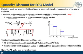
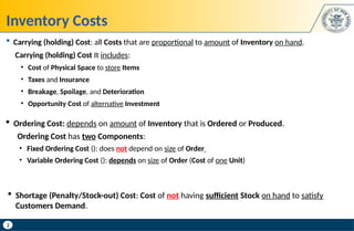
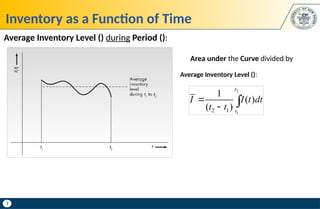
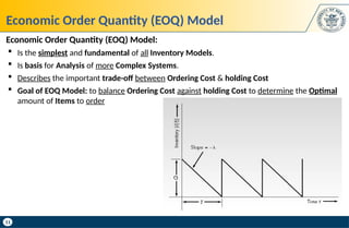
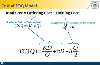
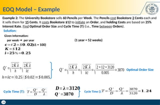
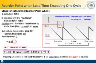
Sensitivity of Cost to Order Quantity Q: Tells us if we order Q instead of Q*, how much it
will affect Annual Cost (i.e., how much more it costs).
𝑇𝐶(𝑄)
𝑇𝐶(𝑄∗
)
=¿
𝐾 𝜆
𝑄
+
h𝑄
2
√2 𝐾 𝜆h
¿
1
2𝑄√2𝐾 𝜆
h
+
𝑄
2 √ h
2𝐾 𝜆
=
𝑄
∗
2𝑄
+
𝑄
2𝑄
∗
=
1
2[𝑄
∗
𝑄
+
𝑄
𝑄
∗ ]
Sensitivity of EOQ Model to Order Quantity Q
𝑇𝐶(𝑄)
𝑇𝐶(𝑄
∗
)
=
1
2 [𝑄
∗
𝑄
+
𝑄
𝑄
∗ ]
 If we order Q: 𝑇𝐶(𝑄)=
𝐾 𝜆
𝑄
+
h𝑄
2
 If we order Q*: 𝑇𝐶(𝑄∗
)=√2𝐾 𝜆h
27
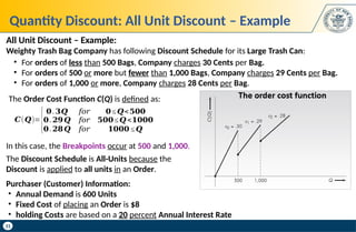
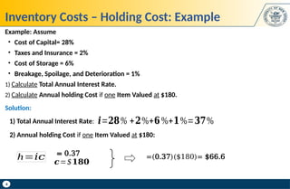
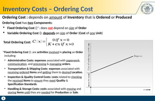
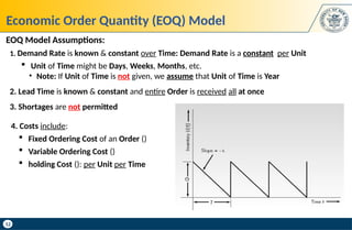
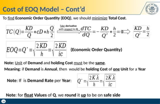
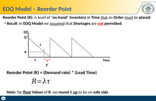
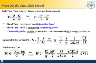
Example: Given an actual size of as twice the size of , how much it will affect
Annual Cost (how much more does it cost)?
Actual size of is twice the size of : 𝑸=𝟐𝑸∗
Interpretation:
The Error made in calculating Annual Cost (i.e., holding and Ordering Costs) as
a result of ordering wrong Value is: 0.25 * 100 = 25%
Meaning: If we order twice as the size of , Annual Cost increases by 25%
Sensitivity of EOQ Model to Order Quantity Q – Example
Solution:
¿
1
2 [1
2
+
2
1 ]
¿
1
2
[2.5]=𝟏.𝟐𝟓
1
2 [ 𝑄
∗
2𝑄
∗
+
2𝑄
∗
𝑄
∗ ]
¿ ¿
𝑸=𝟐𝑸∗
𝑇𝐶(𝑄)
𝑇𝐶(𝑄
∗
)
=
1
2 [𝑄
∗
𝑄
+
𝑄
𝑄
∗ ]
28
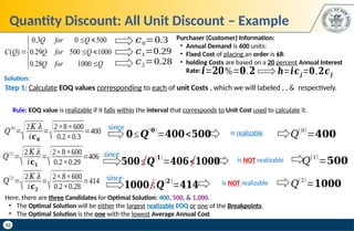
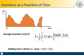
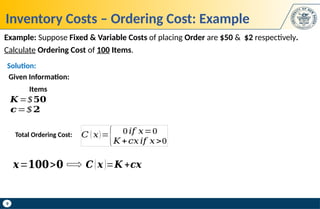
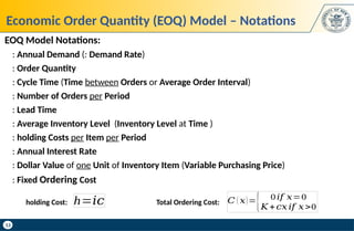
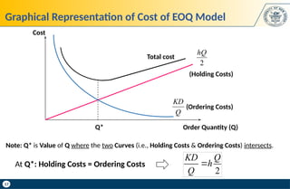
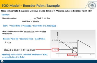
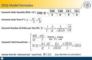
Sensitivity of Cost to Cycle Time T: Tells us how much different values of Time Cycles T (Order
Interval) will affect Annual Cost (i.e., how much more it costs).
Sensitivity of EOQ Model to Time Cycle T (Order Interval)
Annual Cost under 𝑇
Annual Cost under 𝑇
∗
=
𝑇𝐶(𝑇)
𝑇𝐶(𝑇
∗
)
=
1
2 [𝑇
∗
𝑇
+
𝑇
𝑇
∗ ]
𝑻 =
𝑸
𝝀
 If we order Q: 𝑸=𝝀𝑻
𝑻
∗
=
𝑸∗
𝝀
 If we order Q*: 𝑸∗
=𝝀𝑻∗
𝑇𝐶(𝑇 )
𝑇𝐶(𝑇
∗
)
=
1
2 [𝜆𝑇
∗
𝜆𝑇
+
𝜆𝑇
𝜆𝑇
∗ ]=
1
2 [𝑇
∗
𝑇
+
𝑇
𝑇
∗ ]
𝑇𝐶(𝑄)
𝑇𝐶(𝑄
∗
)
=
1
2 [𝑄
∗
𝑄
+
𝑄
𝑄
∗ ]
Sensitivity of EOQ Model to Order Quantity Q:
Sensitivity of EOQ Model to Time Cycle T:
29
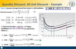
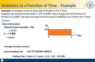
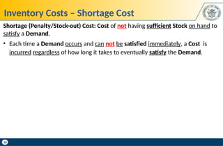
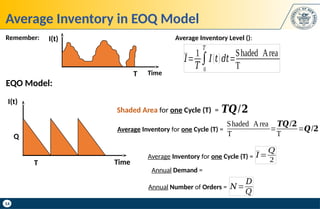
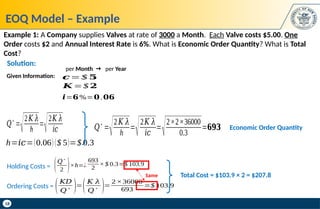
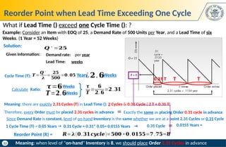
Example: Consider following information
Annual Cost under 𝑇
Annual Cost under 𝑇∗
=
𝑇𝐶(𝑇)
𝑇𝐶(𝑇∗
)
=
1
2 [𝑇
∗
𝑇
+
𝑇
𝑇∗ ]=
1
2 [0.154
0.169
+
0.169
0.154 ]=1.004
Annual Cost under 𝑇=$5916×1.004=$5939.664≈$5940
Now, suppose we have to round Time Cycle T to 8 Weeks. How much it will affect Annual Cost?
𝝀=𝟏𝟎𝟎𝟎
𝑸∗
=𝟏𝟔𝟗
𝑲=$𝟓𝟎𝟎
𝒉=𝟑𝟓
Sensitivity of EOQ Model to Time Cycle T (Order Interval) – Example
𝑻∗
=
𝑸∗
𝝀
=
𝟏𝟔𝟗
𝟏𝟎𝟎𝟎
=𝟎.𝟏𝟔𝟗𝒀𝒆𝒂𝒓𝒔=𝟖.𝟕𝟖𝟖𝑾𝒆𝒆𝒌𝒔
Optimal Time Cycle:
s

Solution:
$5940−$5916=$𝟐𝟒
 Annual Cost increases by:
Annual Cost under
Interpretation: if we round Time Cycle T to 8 Weeks, Annual Cost increases by 0.4%
30
Quantity Discount for EOQ Model
Two Common Quantity Discounts Methods are:
• All Unit Discount: discount is applied to all Units in an Order (All-Units)
• Incremental Discount: discount is applied to additional Units beyond the Breakpoint (Incremental)
Note: The All-Units case is more Common.
Up to this point, we assumed that Purchasing price of each Item () is independent of the size of
the Order.
 However, Suppliers usually charge less per Item for larger Quantity of Orders. Why?
• To encourage Customer to buy the Product in larger Batches.
𝑇𝐶(𝑄)=
𝐾 𝜆
𝑄
+𝑐 𝜆+h
𝑄
2
𝒄𝒋 𝑵𝒋≤𝑸<𝑵𝒋+𝟏 𝒋=𝟎,𝟏,𝟐...𝑱
31
Quantity Discount: All Unit Discount – Example
Purchaser (Customer) Information:
• Annual Demand is 600 Units
• Fixed Cost of placing an Order is $8
• holding Costs are based on a 20 percent Annual Interest Rate
All Unit Discount – Example:
Weighty Trash Bag Company has following Discount Schedule for its Large Trash Can:
• For orders of less than 500 Bags, Company charges 30 Cents per Bag.
• For orders of 500 or more but fewer than 1,000 Bags, Company charges 29 Cents per Bag.
• For orders of 1,000 or more, Company charges 28 Cents per Bag.
𝑪(𝑸)=
{
𝟎.𝟑𝑸 𝑓𝑜𝑟 𝟎≤𝑸<𝟓𝟎𝟎
𝟎.𝟐𝟗𝑸 𝑓𝑜𝑟 𝟓𝟎𝟎≤ 𝑸<𝟏𝟎𝟎𝟎
𝟎.𝟐𝟖𝑸 𝑓𝑜𝑟 𝟏𝟎𝟎𝟎 ≤𝑸
The Order Cost Function C(Q) is defined as:
In this case, the Breakpoints occur at 500 and 1,000.
The Discount Schedule is All-Units because the
Discount is applied to all units in an Order.
32
Quantity Discount: All Unit Discount – Example
0.3 0 500
( ) 0.29 500 1000
0.28 1000
Q for Q
C Q Q for Q
Q for Q
 


  

 

𝑐0=0.3
𝑐1=0.29
𝑐2=0.28
Purchaser (Customer) Information:
• Annual Demand is 600 units:
• Fixed Cost of placing an order is $8:
• holding Costs are based on a 20 percent Annual Interest
Rate:𝒊=𝟐𝟎%=𝟎.𝟐 𝒉=𝒊𝒄𝒋=𝟎.𝟐𝒄𝒋
Step 1: Calculate EOQ values corresponding to each of unit Costs , which we will labeled , , & respectively.
Solution:
Rule: EOQ value is realizable if it falls within the interval that corresponds to Unit Cost used to calculate it.
𝑄
(0)
=
√2𝐾 𝜆
𝑖𝒄𝟎
=
√2×8×600
0.2×0.3
=400 𝟎≤𝑸
(𝟎)
=𝟒𝟎𝟎<𝟓𝟎𝟎
since
is realizable 𝑄
(0)
=𝟒𝟎𝟎
𝑄(1)
=
√2 𝐾 𝜆
𝑖𝒄𝟏
=
√2×8×600
0.2×0.29
=406
𝟓𝟎𝟎≤𝑸(𝟏)
=𝟒𝟎𝟔<𝟏𝟎𝟎𝟎
since
is NOT realizable 𝑄(1)
=𝟓𝟎𝟎
𝑄
(2)
=
√2 𝐾 𝜆
𝑖𝒄𝟐
=
√2×8×600
0.2×0.28
=414
𝟏𝟎𝟎𝟎≤𝑸
(𝟐)
=𝟒𝟏𝟒
since
is NOT realizable 𝑄
(2)
=𝟏𝟎𝟎𝟎
Here, there are three Candidates for Optimal Solution: 400, 500, & 1,000.
• The Optimal Solution will be either the largest realizable EOQ or one of the Breakpoints.
• The Optimal Solution is the one with the lowest Average Annual Cost
33
Quantity Discount: All Unit Discount – Example
Step 2: Calculate Average Annual Cost values for all Candidates.
Total Cost Function: 𝐺 𝑗 (𝑄)=
𝐾 𝜆
𝑄
+𝜆𝑐 𝑗+𝑖𝑐 𝑗
𝑄
2
for
In Total Cost Function, substitute with three
Candidates 400, 500, & 1000 and use appropriate
Values of :
𝐺0 (𝟒𝟎𝟎)=
(600 )( 8)
𝟒𝟎𝟎
+(600) (0.3)+
(0.2 )(0.3 )(𝟒𝟎𝟎)
2
=$ 204.00
𝐺2 (𝟏𝟎𝟎𝟎)=
(600 )(8 )
𝟏𝟎𝟎𝟎
+(600) (0.28)+
(0.2) (0.28 )(𝟏𝟎𝟎𝟎)
2
=$ 200.80
𝐺1 (𝟓𝟎𝟎)=
(600) (8 )
𝟓𝟎𝟎
+(600 )( 0.29)+
(0.2) (0.29) (𝟓𝟎𝟎)
2
=$ 198.10
0.3 0 500
( ) 0.29 500 1000
0.28 1000
Q for Q
C Q Q for Q
Q for Q
 


  

 

𝑐0=0.3
𝑐1=0.29
𝑐2=0.28

𝝀=𝟔𝟎𝟎 𝑲=$𝟖 𝒉=𝒊𝒄𝒋=𝟎.𝟐𝒄𝒋

Inventory Management Il NETWORK DESIGN.pptx

  • 1.
    1 Supply Chain Management INDE6641 Inventory Management (II) Economic Order Quantity (EOQ) Dr. Narjes Sadeghiamirshahidi Department of Mechanical and Industrial Engineering Copyright © 2015 by Steven Nahmias and Tava Lennon Olsen. All Rights Reserved
  • 2.
    2 Inventory Costs  Carrying(holding) Cost: all Costs that are proportional to amount of Inventory on hand. Carrying (holding) Cost It includes: • Cost of Physical Space to store Items • Taxes and Insurance • Breakage, Spoilage, and Deterioration • Opportunity Cost of alternative Investment  Ordering Cost: depends on amount of Inventory that is Ordered or Produced. Ordering Cost has two Components: • Fixed Ordering Cost (): does not depend on size of Order • Variable Ordering Cost (): depends on size of Order (Cost of one Unit)  Shortage (Penalty/Stock-out) Cost: Cost of not having sufficient Stock on hand to satisfy Customers Demand.
  • 3.
    3 Inventory Costs –Holding Cost Carrying (holding) Cost is based on average Inventory level Annual Interest Rate () commonly includes four Components:  Cost of Capital  Taxes and Insurance  Cost of Storage  Breakage, Spoilage, and Deterioration : Annual holding Cost (Dollar per Unit) : Annual Interest Rate : Dollar Value of one Unit of Inventory h=𝑖𝑐
  • 4.
    4 Inventory Costs –Holding Cost: Example Example: Assume • Cost of Capital= 28% • Taxes and Insurance = 2% • Cost of Storage = 6% • Breakage, Spoilage, and Deterioration = 1% 1) Calculate Total Annual Interest Rate. 2) Calculate Annual holding Cost if one Item Valued at $180. 𝒊=𝟐𝟖% +𝟐%+𝟔%+𝟏%=𝟑𝟕% 1) Total Annual Interest Rate: Solution: 2) Annual holding Cost if one Item Valued at $180: h=𝑖𝑐 =(0.37)($180)= $66.6 = 0.37 𝒄=$𝟏𝟖𝟎
  • 5.
    5 Inventory as aFunction of Time Holding Cost of Items for years = ()()() = ()()() I(t ) Time T 0 𝐼= 1 𝑇 ∫ 0 𝑇 𝐼(𝑡) 𝑑𝑡= Shaded Area T Average Inventory Level ():
  • 6.
    6 Inventory as aFunction of Time – Example Example: A Company wants to keep 300 of Product A for 5 Years. Suppose the Annual Interest Rate is 37% & Dollar Value of one Unit of Inventory of Product A is $180. Calculate Average Inventory Level & Holding Cost of Items for 5 Years. I(t) Time 5 300 0 Holding Cost of items for 5 years = ()()() =)()() = $99,900 Average Inventory Level (): Given Information: = 0.37 = 5 years 𝒄=$𝟏𝟖𝟎 Desired Product Quantity = 300 =(0.37)($180)=$66.6 Annual holding Cost: Solution:
  • 7.
    7 Inventory as aFunction of Time Average Inventory Level () during Period (): 2 1 2 1 1 ( ) ( ) t t I I t dt t t    Area under the Curve divided by Average Inventory Level ():
  • 8.
    8 Inventory Costs –Ordering Cost Ordering Cost : depends on amount of Inventory that is Ordered or Produced Ordering Cost has two Components:  Fixed Ordering Cost ()*: does not depend on size of Order  Variable Ordering Cost (): depends on size of Order (Cost of one Unit) 𝐶 ( 𝑥)={ 0 𝑖𝑓 𝑥=0 𝐾 +𝑐𝑥 𝑖𝑓 𝑥 >0 Total Ordering Cost: *Fixed Ordering Cost (): are activities involved in placing an Order including: • Administrative Costs: expenses associated with paperwork, communication, and processing & managing orders. • Transportation & Shipping Costs: expenses associated with receiving ordered Items and getting them to desired Location. • Inspection & Quality Control Costs: costs related to checking the received Items to ensure they meet Quality & Specification Standards. • Handling & Storage Costs: costs associated with moving and storing Items until they are needed for Production or Sale.
  • 9.
    9 Inventory Costs –Ordering Cost: Example 𝐶 ( 𝑥)= { 0𝑖𝑓 𝑥=0 𝐾+𝑐𝑥 𝑖𝑓 𝑥>0 Total Ordering Cost: Example: Suppose Fixed & Variable Costs of placing Order are $50 & $2 respectively. Calculate Ordering Cost of 100 Items. 𝑲 =$𝟓𝟎 Given Information: 𝒄=$ 𝟐 Items 𝒙=𝟏𝟎𝟎>𝟎 𝑪(𝒙)=𝑲 +𝒄𝒙 Solution:
  • 10.
    10 Inventory Costs –Shortage Cost Shortage (Penalty/Stock-out) Cost: Cost of not having sufficient Stock on hand to satisfy a Demand. • Each time a Demand occurs and can not be satisfied immediately, a Cost is incurred regardless of how long it takes to eventually satisfy the Demand.
  • 11.
    11 Economic Order Quantity(EOQ) Model Economic Order Quantity (EOQ) Model:  Is the simplest and fundamental of all Inventory Models.  Is basis for Analysis of more Complex Systems.  Describes the important trade-off between Ordering Cost & holding Cost  Goal of EOQ Model: to balance Ordering Cost against holding Cost to determine the Optimal amount of Items to order
  • 12.
    12 Economic Order Quantity(EOQ) Model EOQ Model Assumptions: 1. Demand Rate is known & constant over Time: Demand Rate is a constant per Unit  Unit of Time might be Days, Weeks, Months, etc. • Note: If Unit of Time is not given, we assume that Unit of Time is Year 2. Lead Time is known & constant and entire Order is received all at once 3. Shortages are not permitted 4. Costs include:  Fixed Ordering Cost of an Order ()  Variable Ordering Cost ()  holding Cost (): per Unit per Time
  • 13.
    13 Economic Order Quantity(EOQ) Model – Notations EOQ Model Notations: : Annual Demand (: Demand Rate) : Order Quantity : Cycle Time (Time between Orders or Average Order Interval) : Number of Orders per Period : Lead Time : Average Inventory Level (Inventory Level at Time ) : holding Costs per Item per Period : Annual Interest Rate : Dollar Value of one Unit of Inventory Item (Variable Purchasing Price) : Fixed Ordering Cost holding Cost: h=𝑖𝑐 Total Ordering Cost: 𝐶 ( 𝑥)= { 0 𝑖𝑓 𝑥=0 𝐾 +𝑐𝑥 𝑖𝑓 𝑥>0
  • 14.
    14 Average Inventory inEOQ Model I(t) Time T Q Shaded Area for one Cycle (T) = 𝑻𝑸/𝟐 Annual Demand = EQO Model: Average Inventory for one Cycle (T) = 𝐼= 𝑄 2 Annual Number of Orders = 𝑁= 𝐷 𝑄 Remember: I(t) Time T 𝐼= 1 𝑇 ∫ 0 𝑇 𝐼(𝑡)𝑑𝑡= Shaded Area T Average Inventory Level (): Average Inventory for one Cycle (T) = Shaded Area T = 𝑻𝑸/𝟐 T =𝑸/𝟐
  • 15.
    15 Cost of EOQModel Total Cost = Ordering Cost + Holding Cost 𝑇𝐶(𝑄)= 𝐾𝐷 𝑄 +𝑐𝐷 +h 𝑄 2 Number of Orders × Ordering Cost (𝐷/𝑄)×(𝐾 +𝑐𝑄) Average Inventory () × holding Costs per item per period ( 𝑄 2 )× h
  • 16.
    16 Cost of EOQModel – Cont’d 𝑇𝐶(𝑄)= 𝐾𝐷 𝑄 +𝑐𝐷+h 𝑄 2 𝑑𝑇𝐶 𝑑𝑄 =− 𝐾𝐷 𝑄 2 + h 2 =0 𝐾𝐷 𝑄 2 = h 2 Note: If is Demand Rate per Year: 𝑄 ∗ = √2𝐾 𝜆 h = √2𝐾 𝜆 𝑖𝑐 𝐸𝑂𝑄=𝑄 ∗ = √2𝐾𝐷 h = √2𝐾𝐷 𝑖𝑐 (Economic Order Quantity) To find Economic Order Quantity (EOQ), we should minimize Total Cost. Take derivative with respect to Q Note: Unit of Demand and holding Cost must be the same. Meaning: if Demand is Annual, then would be holding Cost of one Unit for a Year Note: for float Values of Q, we round it up to be on safe side
  • 17.
    17 Graphical Representation ofCost of EOQ Model Note: Q* is Value of Q where the two Curves (i.e., Holding Costs & Ordering Costs) intersects. At Q*: Holding Costs = Ordering Costs 2 KD Q h Q  (Holding Costs) Cost Order Quantity (Q) Q* Total cost (Ordering Costs) 2 hQ Q KD
  • 18.
    18 EOQ Model –Example Example 1: A Company supplies Valves at rate of 3000 a Month. Each Valve costs $5.00. One Order costs $2 and Annual Interest Rate is 6%. What is Economic Order Quantity? What is Total Cost? 𝑲 =$ 𝟐 per Month  per Year 𝒄= $ 𝟓 𝒊=𝟔%=𝟎.𝟎𝟔 Given Information: Solution: 𝑄∗ = √2𝐾 𝜆 h = √2𝐾 𝜆 𝑖𝑐 h=𝑖𝑐=(0.06) ($ 5)=$ 0.3 𝑄∗ = √2𝐾 𝜆 h = √2𝐾 𝜆 𝑖𝑐 = √2×2×36000 0.3 =𝟔𝟗𝟑 Economic Order Quantity Total Cost = $103.9 × 2 = $207.8 Holding Costs = 693 2 × $ 0.3=$ 103.9 (𝑄∗ 2 )×h=¿ Ordering Costs = (𝐾𝐷 𝑄 ∗ )= (𝐾 𝜆 𝑄 ∗ )= 2 ×36000 693 =$ 103.9 Same
  • 19.
    19 EOQ Model –Example Example 2: The University Bookstore sells 60 Pencils per Week. The Pencils cost Bookstore 2 Cents each and it sells them for 15 Cents. It costs Bookstore $12 to initiate an Order, and holding Costs are based on 25% Interest Rate. Find Optimal Order Size and Cycle Time (T) (i.e., Time between Orders). 𝑄 ∗ = √2𝐾 𝜆 h = √2𝐾 𝜆 𝑖𝑐 h=𝑖𝑐=(0.25)($ 0.02)=$ 0.005 𝑄 ∗ = √2𝐾 𝜆 h = √2𝐾 𝜆 𝑖𝑐 = √2×12×3120 0.005 =3870 Optimal Order Size 𝑲 =$𝟏𝟐 per week  per year 𝒄=¢ 𝟐=$ 𝟎. 𝟎𝟐 𝒊=𝟐𝟓%=𝟎.𝟐𝟓 Given Information: (1 year = 52 weeks) ($1 = 100) 𝑇 = 𝑄∗ 𝐷 = 𝑄∗ 𝜆 = 3870 3120 =𝟏 . 𝟐𝟒 𝑫=𝝀=𝟑𝟏𝟐𝟎 𝑸∗ =𝟑𝟖𝟕𝟎 Cycle Time (): Cycle Time (T): 𝑇 = 𝑄∗ 𝐷 = 𝑄∗ 𝜆 Solution:
  • 20.
    20 EOQ Model –Reorder Point I(t) Time T Q* -l  R Reorder Point (R): is level of "on-hand" Inventory at Time that an Order must be placed. • Recall: In EOQ Model we assumed that Shortages are not permitted. Reorder Point (R) = (Demand rate) * (Lead Time) 𝑅=𝜆𝜏 Note: for float Values of R, we round it up to be on safe side
  • 21.
    21 EOQ Model –Reorder Point: Example Now, in Example 2, suppose we have a Lead Time of 4 Months. What is Reorder Point (R)? 𝑅=𝜆𝜏=3120×0.3333=1040 Meaning: when level of "on-hand" Inventory is 1040, we should place the Order Reorder Point (R) = (Demand rate) * (Lead Time) 𝑅=𝜆𝜏 Lead Time  Months per Week  per Year Given Information: Note: all relevant Variables always should be in the same Unit of Time. Years  Lead Time of 4 Months = Lead Time of 0.3333 Years Solution:
  • 22.
    22 Reorder Point whenLead Time Exceeding One Cycle What if Lead Time () exceed one Cycle Time (): ? Example: Consider an Item with EOQ of 25, a Demand Rate of 500 Units per Year, and a Lead Time of six Weeks. (1 Year = 52 Weeks) 𝑸∗ =𝟐𝟓 per year Demand rate: weeks Lead Time: Given Information: Meaning: there are exactly 2.31 Cycles (T) in Lead Time (): 2 Cycles & 0.31 Cycle ( 2 T + 0.31 T) Therefore, every Order must be placed 2.31 cycles in advance ≡ Exactly the same as placing Order 0.31 cycle in advance Since Demand Rate is constant, level of on-hand Inventory is the same whether we are at a point 2.31 Cycles or 0.31 Cycle 𝑹= 𝝀(𝟎.𝟑𝟏𝒄𝒚𝒄𝒍𝒆)=𝟓𝟎𝟎×𝟎.𝟎𝟏𝟓𝟓=𝟕.𝟕𝟓≈𝟖 Reorder Point (R) = T T 0.31 T Solution: 𝑻= 𝑸∗ 𝝀 = 𝟐𝟓 𝟓𝟎𝟎 =𝟎.𝟎𝟓 Cycle Time (T): ¿𝟐.𝟔 Years Weeks Calculate Ratio: 𝝉=𝟔 𝑻=𝟐.𝟔 𝝉 𝑻 = 𝟔 𝟐.𝟔 =𝟐.𝟑𝟏 Weeks Weeks 1 Cycle Time (T) = 0.05 Years  0.31 Cycle = 0.31* 0.05= 0.0155 Years  0.31 Cycle ≡ 0.0155 Years = Meaning: when level of "on-hand" Inventory is 8, we should place Order 2.31 Cycles in advance
  • 23.
    23 Steps for calculatingReorder Point when : 1. Calculate Ratio. Reorder Point when Lead Time Exceeding One Cycle 2. Consider only the "fractional" Remainder of Ratio. Multiply this "fractional" Remainder by Cycle Time (T) to convert it to years. 3. Multiply the result of Step 2 by Demand Rate () to get Reorder Point () 𝑹= 𝝀(𝟎.𝟑𝟏𝒄𝒚𝒄𝒍𝒆)=𝟓𝟎𝟎×𝟎.𝟎𝟏𝟓𝟓=𝟕.𝟕𝟓≈𝟖 =500/year, Q=25, =6 weeks =25/500=0.05 (2.6 weeks) Given Information: = 2.31 0.31* 0.05 = 0.0155 Years Meaning: when level of "on-hand" Inventory is 8, we should place the Order 2.31 Cycles in advance
  • 24.
    24 More Details aboutEOQ Model Cycle Time (Time between Orders or Average Order Interval): 𝑻= 𝑸 𝝀 = 𝑸 𝑫  If Lead Time : there is only one Outstanding Order*  If Lead Time : there is at least one Outstanding Order* *Outstanding Order: Number of Items that have been ordered but have not received yet. 𝑻∗ = 𝑸∗ 𝝀 = 𝑸∗ 𝑫 For Number of Orders per Year (N): 𝑵 ∗ = 𝟏 𝑻 ∗ = 𝝀 𝑸 ∗ = 𝝀 √𝟐𝑲 𝝀/𝒉 = √𝝀𝒉 𝟐𝑲 𝑵= 𝟏 𝑻 = 𝝀 𝑸 For Total Annual Cost: 𝑻𝑪(𝑸 ∗ )= 𝑲 𝝀 𝑸 ∗ + 𝒉𝑸∗ 𝟐 = 𝑲 𝝀 √𝟐𝑲 𝝀/𝒉 + 𝒉√𝟐𝑲 𝝀/𝒉 𝟐 =√𝟐𝑲 𝝀𝒉 𝑻𝑪(𝑸)= 𝑲 𝝀 𝑸 + 𝒉𝑸 𝟐 For
  • 25.
    25 EOQ Model Formulas EconomicCycle Time (T*): 𝑇 ∗ = 𝑄∗ 𝜆 = 𝑄∗ 𝐷 Reorder Point (R) = (Demand rate) * (Lead Time) 𝑅=𝜆𝜏 Economic Number of Orders per Year (N): 𝑁 ∗ = 1 𝑇 ∗ = 𝜆 𝑄 ∗ = 𝜆 √2𝐾 𝜆/h = √𝜆h 2𝐾 Economic Total Annual Cost: 𝐾𝐷 𝑄 ∗ = h𝑄∗ 2 ¿Holding Cost Ordering Cost 𝑇𝐶(𝑄 ∗ )= 𝐾 𝜆 𝑄 ∗ + h𝑄∗ 2 = 𝐾 𝜆 √2𝐾 𝜆/h + h√2𝐾 𝜆/h 2 =√2𝐾 𝜆h (pay attention to calculation) 𝑬𝑶𝑸=𝑸∗ = √𝟐𝑲𝑫 𝒉 = √𝟐𝑲𝑫 𝒊𝒄 = √𝟐𝑲 𝝀 𝒉 = √𝟐𝑲 𝝀 𝒊𝒄 Economic Order Quantity (EOQ = Q*):
  • 26.
    26 Sensitivity of Costto Order Quantity Q: Tells us if we order Q instead of Q*, how much it will affect Annual Cost (i.e., how much more it costs). 𝑇𝐶(𝑄) 𝑇𝐶(𝑄∗ ) =¿ 𝐾 𝜆 𝑄 + h𝑄 2 √2 𝐾 𝜆h ¿ 1 2𝑄√2𝐾 𝜆 h + 𝑄 2 √ h 2𝐾 𝜆 = 𝑄 ∗ 2𝑄 + 𝑄 2𝑄 ∗ = 1 2[𝑄 ∗ 𝑄 + 𝑄 𝑄 ∗ ] Sensitivity of EOQ Model to Order Quantity Q 𝑇𝐶(𝑄) 𝑇𝐶(𝑄 ∗ ) = 1 2 [𝑄 ∗ 𝑄 + 𝑄 𝑄 ∗ ]  If we order Q: 𝑇𝐶(𝑄)= 𝐾 𝜆 𝑄 + h𝑄 2  If we order Q*: 𝑇𝐶(𝑄∗ )=√2𝐾 𝜆h
  • 27.
    27 Example: Given anactual size of as twice the size of , how much it will affect Annual Cost (how much more does it cost)? Actual size of is twice the size of : 𝑸=𝟐𝑸∗ Interpretation: The Error made in calculating Annual Cost (i.e., holding and Ordering Costs) as a result of ordering wrong Value is: 0.25 * 100 = 25% Meaning: If we order twice as the size of , Annual Cost increases by 25% Sensitivity of EOQ Model to Order Quantity Q – Example Solution: ¿ 1 2 [1 2 + 2 1 ] ¿ 1 2 [2.5]=𝟏.𝟐𝟓 1 2 [ 𝑄 ∗ 2𝑄 ∗ + 2𝑄 ∗ 𝑄 ∗ ] ¿ ¿ 𝑸=𝟐𝑸∗ 𝑇𝐶(𝑄) 𝑇𝐶(𝑄 ∗ ) = 1 2 [𝑄 ∗ 𝑄 + 𝑄 𝑄 ∗ ]
  • 28.
    28 Sensitivity of Costto Cycle Time T: Tells us how much different values of Time Cycles T (Order Interval) will affect Annual Cost (i.e., how much more it costs). Sensitivity of EOQ Model to Time Cycle T (Order Interval) Annual Cost under 𝑇 Annual Cost under 𝑇 ∗ = 𝑇𝐶(𝑇) 𝑇𝐶(𝑇 ∗ ) = 1 2 [𝑇 ∗ 𝑇 + 𝑇 𝑇 ∗ ] 𝑻 = 𝑸 𝝀  If we order Q: 𝑸=𝝀𝑻 𝑻 ∗ = 𝑸∗ 𝝀  If we order Q*: 𝑸∗ =𝝀𝑻∗ 𝑇𝐶(𝑇 ) 𝑇𝐶(𝑇 ∗ ) = 1 2 [𝜆𝑇 ∗ 𝜆𝑇 + 𝜆𝑇 𝜆𝑇 ∗ ]= 1 2 [𝑇 ∗ 𝑇 + 𝑇 𝑇 ∗ ] 𝑇𝐶(𝑄) 𝑇𝐶(𝑄 ∗ ) = 1 2 [𝑄 ∗ 𝑄 + 𝑄 𝑄 ∗ ] Sensitivity of EOQ Model to Order Quantity Q: Sensitivity of EOQ Model to Time Cycle T:
  • 29.
    29 Example: Consider followinginformation Annual Cost under 𝑇 Annual Cost under 𝑇∗ = 𝑇𝐶(𝑇) 𝑇𝐶(𝑇∗ ) = 1 2 [𝑇 ∗ 𝑇 + 𝑇 𝑇∗ ]= 1 2 [0.154 0.169 + 0.169 0.154 ]=1.004 Annual Cost under 𝑇=$5916×1.004=$5939.664≈$5940 Now, suppose we have to round Time Cycle T to 8 Weeks. How much it will affect Annual Cost? 𝝀=𝟏𝟎𝟎𝟎 𝑸∗ =𝟏𝟔𝟗 𝑲=$𝟓𝟎𝟎 𝒉=𝟑𝟓 Sensitivity of EOQ Model to Time Cycle T (Order Interval) – Example 𝑻∗ = 𝑸∗ 𝝀 = 𝟏𝟔𝟗 𝟏𝟎𝟎𝟎 =𝟎.𝟏𝟔𝟗𝒀𝒆𝒂𝒓𝒔=𝟖.𝟕𝟖𝟖𝑾𝒆𝒆𝒌𝒔 Optimal Time Cycle: s  Solution: $5940−$5916=$𝟐𝟒  Annual Cost increases by: Annual Cost under Interpretation: if we round Time Cycle T to 8 Weeks, Annual Cost increases by 0.4%
  • 30.
    30 Quantity Discount forEOQ Model Two Common Quantity Discounts Methods are: • All Unit Discount: discount is applied to all Units in an Order (All-Units) • Incremental Discount: discount is applied to additional Units beyond the Breakpoint (Incremental) Note: The All-Units case is more Common. Up to this point, we assumed that Purchasing price of each Item () is independent of the size of the Order.  However, Suppliers usually charge less per Item for larger Quantity of Orders. Why? • To encourage Customer to buy the Product in larger Batches. 𝑇𝐶(𝑄)= 𝐾 𝜆 𝑄 +𝑐 𝜆+h 𝑄 2 𝒄𝒋 𝑵𝒋≤𝑸<𝑵𝒋+𝟏 𝒋=𝟎,𝟏,𝟐...𝑱
  • 31.
    31 Quantity Discount: AllUnit Discount – Example Purchaser (Customer) Information: • Annual Demand is 600 Units • Fixed Cost of placing an Order is $8 • holding Costs are based on a 20 percent Annual Interest Rate All Unit Discount – Example: Weighty Trash Bag Company has following Discount Schedule for its Large Trash Can: • For orders of less than 500 Bags, Company charges 30 Cents per Bag. • For orders of 500 or more but fewer than 1,000 Bags, Company charges 29 Cents per Bag. • For orders of 1,000 or more, Company charges 28 Cents per Bag. 𝑪(𝑸)= { 𝟎.𝟑𝑸 𝑓𝑜𝑟 𝟎≤𝑸<𝟓𝟎𝟎 𝟎.𝟐𝟗𝑸 𝑓𝑜𝑟 𝟓𝟎𝟎≤ 𝑸<𝟏𝟎𝟎𝟎 𝟎.𝟐𝟖𝑸 𝑓𝑜𝑟 𝟏𝟎𝟎𝟎 ≤𝑸 The Order Cost Function C(Q) is defined as: In this case, the Breakpoints occur at 500 and 1,000. The Discount Schedule is All-Units because the Discount is applied to all units in an Order.
  • 32.
    32 Quantity Discount: AllUnit Discount – Example 0.3 0 500 ( ) 0.29 500 1000 0.28 1000 Q for Q C Q Q for Q Q for Q            𝑐0=0.3 𝑐1=0.29 𝑐2=0.28 Purchaser (Customer) Information: • Annual Demand is 600 units: • Fixed Cost of placing an order is $8: • holding Costs are based on a 20 percent Annual Interest Rate:𝒊=𝟐𝟎%=𝟎.𝟐 𝒉=𝒊𝒄𝒋=𝟎.𝟐𝒄𝒋 Step 1: Calculate EOQ values corresponding to each of unit Costs , which we will labeled , , & respectively. Solution: Rule: EOQ value is realizable if it falls within the interval that corresponds to Unit Cost used to calculate it. 𝑄 (0) = √2𝐾 𝜆 𝑖𝒄𝟎 = √2×8×600 0.2×0.3 =400 𝟎≤𝑸 (𝟎) =𝟒𝟎𝟎<𝟓𝟎𝟎 since is realizable 𝑄 (0) =𝟒𝟎𝟎 𝑄(1) = √2 𝐾 𝜆 𝑖𝒄𝟏 = √2×8×600 0.2×0.29 =406 𝟓𝟎𝟎≤𝑸(𝟏) =𝟒𝟎𝟔<𝟏𝟎𝟎𝟎 since is NOT realizable 𝑄(1) =𝟓𝟎𝟎 𝑄 (2) = √2 𝐾 𝜆 𝑖𝒄𝟐 = √2×8×600 0.2×0.28 =414 𝟏𝟎𝟎𝟎≤𝑸 (𝟐) =𝟒𝟏𝟒 since is NOT realizable 𝑄 (2) =𝟏𝟎𝟎𝟎 Here, there are three Candidates for Optimal Solution: 400, 500, & 1,000. • The Optimal Solution will be either the largest realizable EOQ or one of the Breakpoints. • The Optimal Solution is the one with the lowest Average Annual Cost
  • 33.
    33 Quantity Discount: AllUnit Discount – Example Step 2: Calculate Average Annual Cost values for all Candidates. Total Cost Function: 𝐺 𝑗 (𝑄)= 𝐾 𝜆 𝑄 +𝜆𝑐 𝑗+𝑖𝑐 𝑗 𝑄 2 for In Total Cost Function, substitute with three Candidates 400, 500, & 1000 and use appropriate Values of : 𝐺0 (𝟒𝟎𝟎)= (600 )( 8) 𝟒𝟎𝟎 +(600) (0.3)+ (0.2 )(0.3 )(𝟒𝟎𝟎) 2 =$ 204.00 𝐺2 (𝟏𝟎𝟎𝟎)= (600 )(8 ) 𝟏𝟎𝟎𝟎 +(600) (0.28)+ (0.2) (0.28 )(𝟏𝟎𝟎𝟎) 2 =$ 200.80 𝐺1 (𝟓𝟎𝟎)= (600) (8 ) 𝟓𝟎𝟎 +(600 )( 0.29)+ (0.2) (0.29) (𝟓𝟎𝟎) 2 =$ 198.10 0.3 0 500 ( ) 0.29 500 1000 0.28 1000 Q for Q C Q Q for Q Q for Q            𝑐0=0.3 𝑐1=0.29 𝑐2=0.28  𝝀=𝟔𝟎𝟎 𝑲=$𝟖 𝒉=𝒊𝒄𝒋=𝟎.𝟐𝒄𝒋