Download as PDF, PPTX


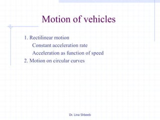

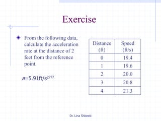
![Dr. Lina Shbeeb
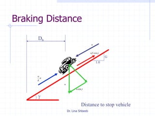
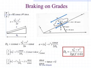
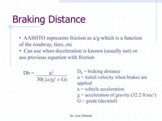
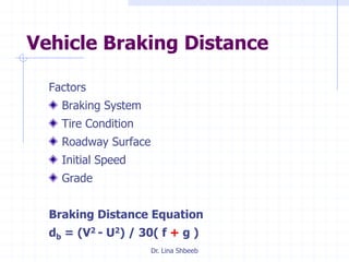
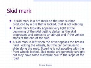
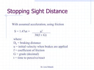
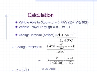
Braking distance
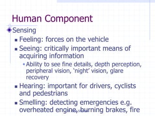
Braking Distance (Db)
Db = distance from brakes enact to final speed
Db = f(velocity, grade, friction)
Db = (V0
2 – V2)/[30(f +/- G)]
or
Db = (V0
2 – V2)/[254(f +/- G)] metric
Db = braking distance (feet or meters)
V0 = initial velocity (mph or kph)
V = final velocity (mph or kph)
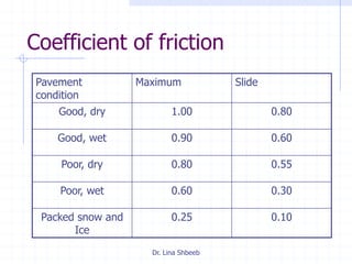
f = coefficient of friction
G = Grade (decimal)
30 or 254 = conversion coefficient](https://image.slidesharecdn.com/drivervehicle-160630235101/85/Driver-Vehicle-Transportation-Engineering-Dr-Lina-Shbeeb-48-320.jpg)
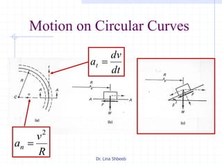
![Dr. Lina Shbeeb
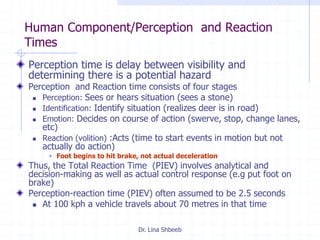
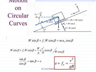
Minimum Radius of a Circular Curve
where u = vehicle velocity (mph)
e = tan (rate of superelevation)
fs = coefficient of side friction (depends on design speed)
Example
design speed = 65 mph
rate of superelevation = 0.05
coefficient of side friction = 0.11
Solution
minimum radius
R = (65)2/[15(0.05+0.11)] = 1760 ft
)(15
2
sfe
u
R
](https://image.slidesharecdn.com/drivervehicle-160630235101/85/Driver-Vehicle-Transportation-Engineering-Dr-Lina-Shbeeb-62-320.jpg)
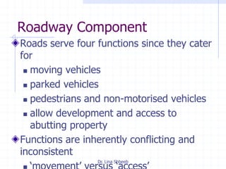

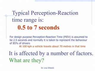
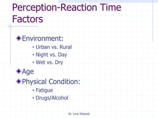
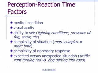
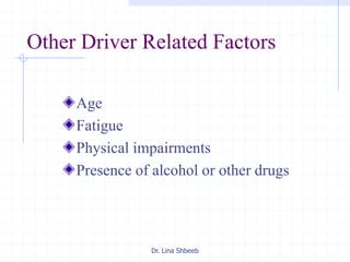
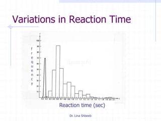
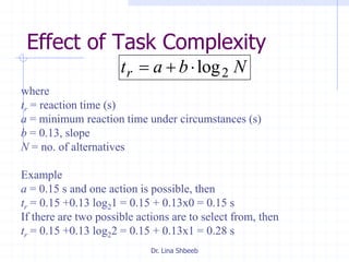
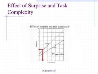
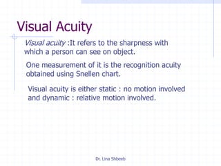
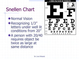
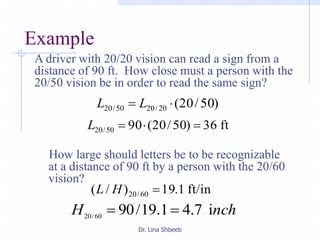
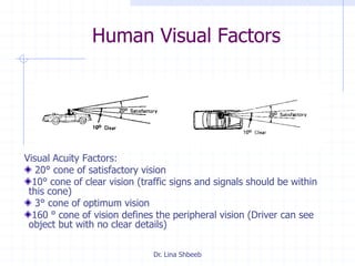
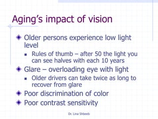
The document discusses several key aspects of the human component in transportation systems. It describes humans as one of the three main components of traffic systems, along with roadways and vehicles. Humans act as drivers, passengers, pedestrians, and cyclists. The document outlines factors that influence perception-reaction times, such as age, environment, visual acuity, and complexity of the situation. It also discusses design considerations for factors like road sign legibility and vehicle characteristics that affect road design.


![02-A Components of Traffic System [Road Users and Vehicles] (Traffic Engineer...](https://cdn.slidesharecdn.com/ss_thumbnails/02acomponentsoftsroadusersvehicles-200412120058-thumbnail.jpg?width=640&height=640&fit=bounds)


![11 Geometric Design of Railway Track [Vertical Alignment] (Railway Engineerin...](https://cdn.slidesharecdn.com/ss_thumbnails/geometricdesignofrailwaytrack-ii-200415172410-thumbnail.jpg?width=640&height=640&fit=bounds)
![10 Geometric Design of Railway Track [Horizontal Alignment] (Railway Engineer...](https://cdn.slidesharecdn.com/ss_thumbnails/geometricdesignofrailwaytrack-i-200415171932-thumbnail.jpg?width=640&height=640&fit=bounds)


