Downloaded 219 times

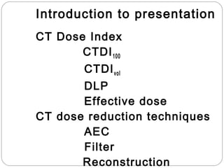


1) CT dose index (CTDI) measures radiation output of CT scanners. Modern measures include CTDI100, CTDIvol, and dose length product (DLP). 2) Automatic exposure control (AEC) modulates tube current based on patient attenuation to maintain consistent image quality while reducing dose. 3) Dose reduction techniques in CT include AEC, bowtie filters, iterative reconstruction, prospective gating, and dynamic collimation.