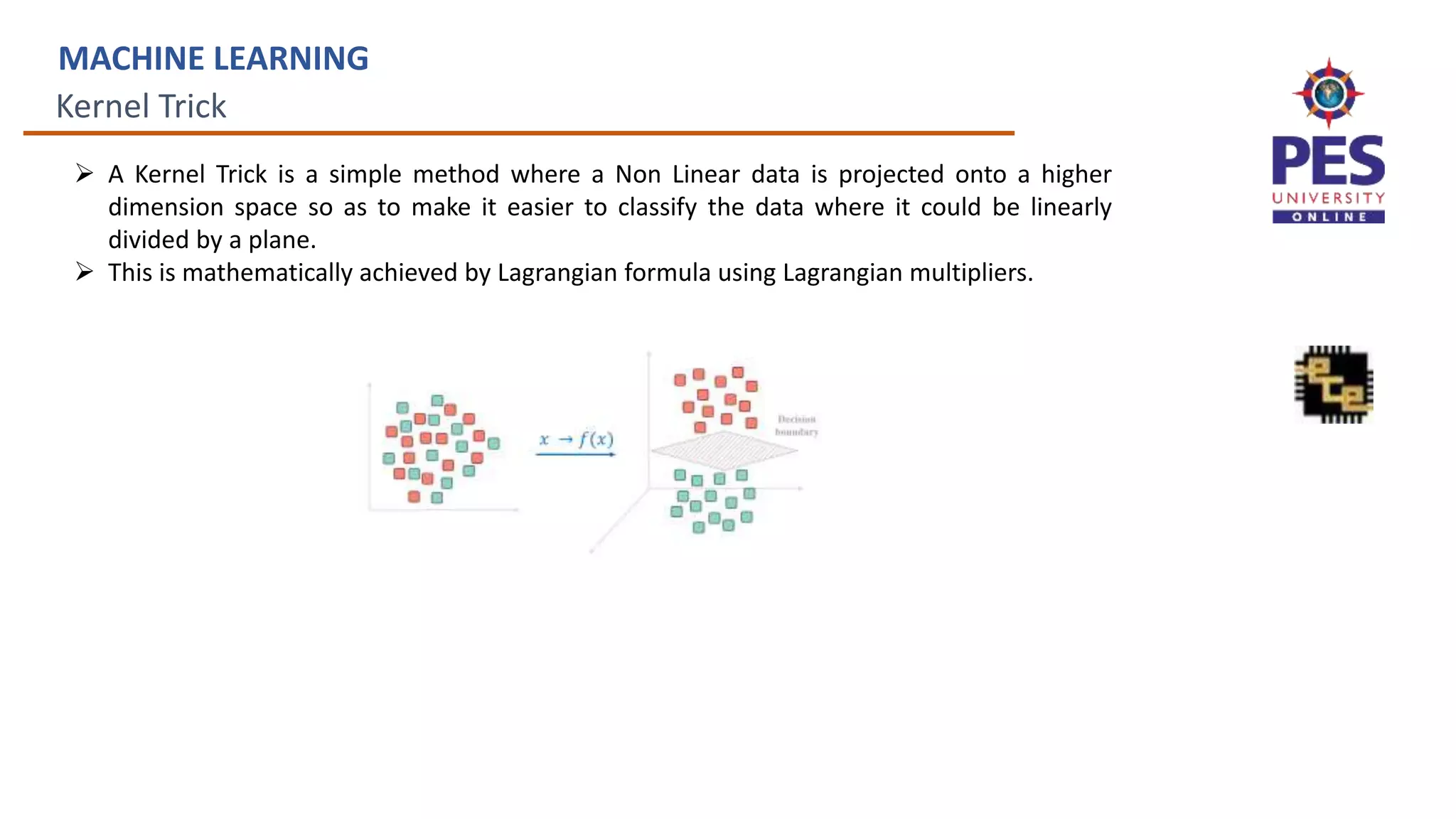
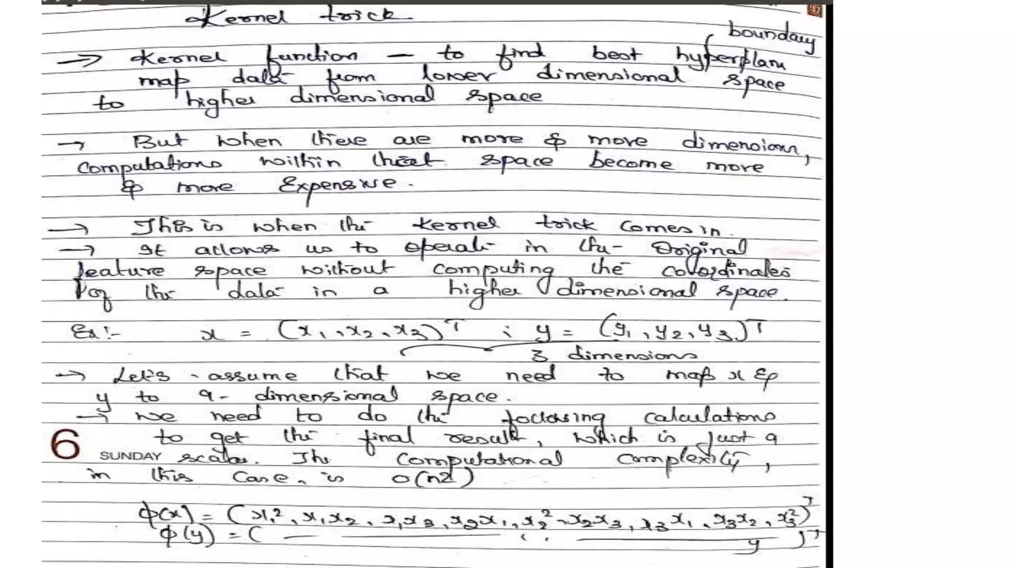
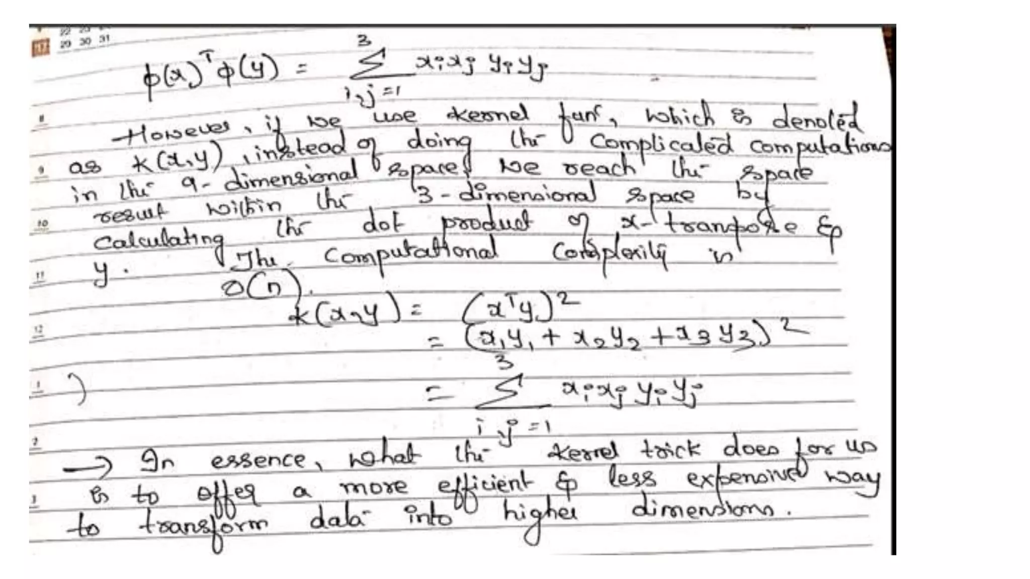
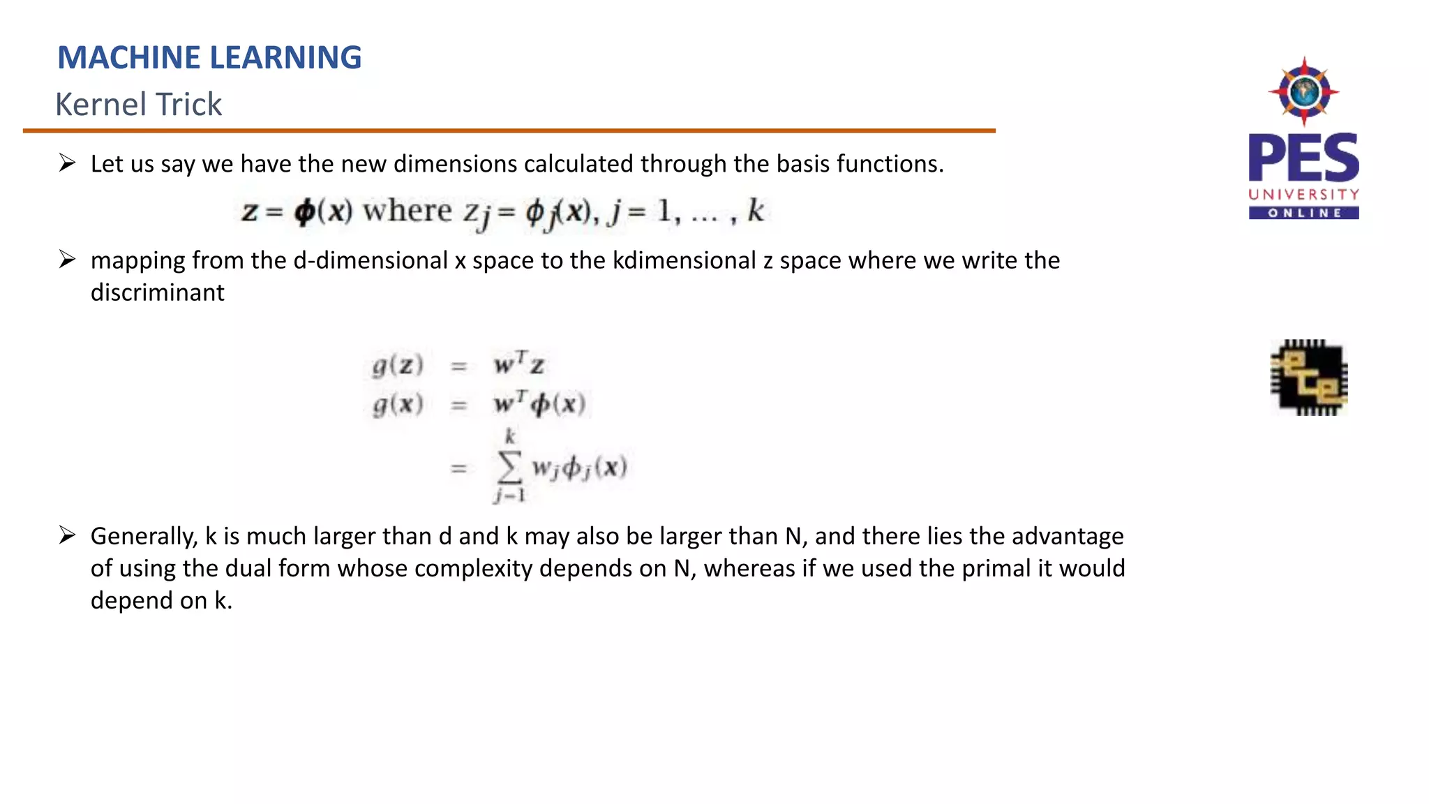
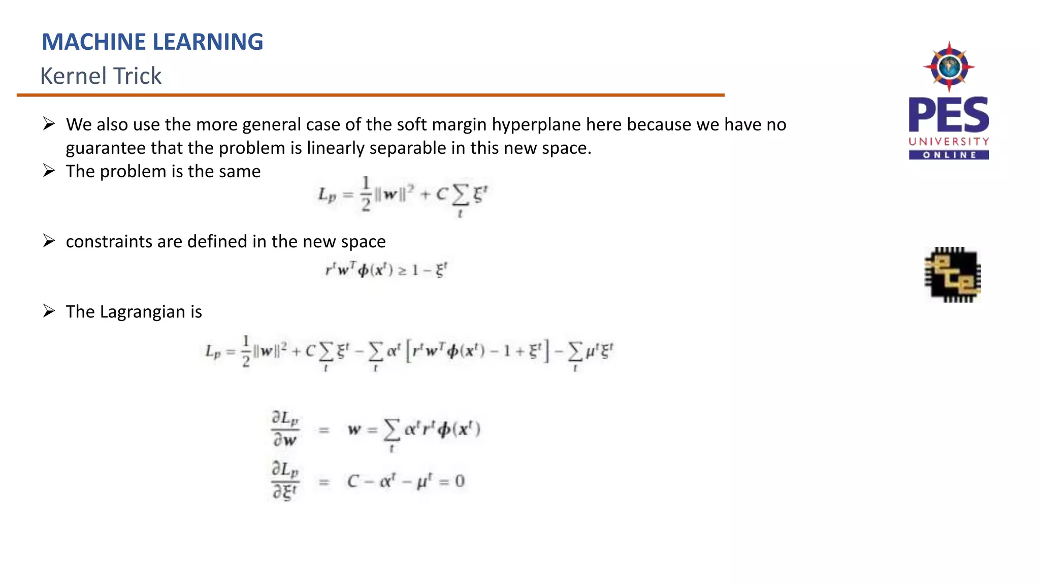
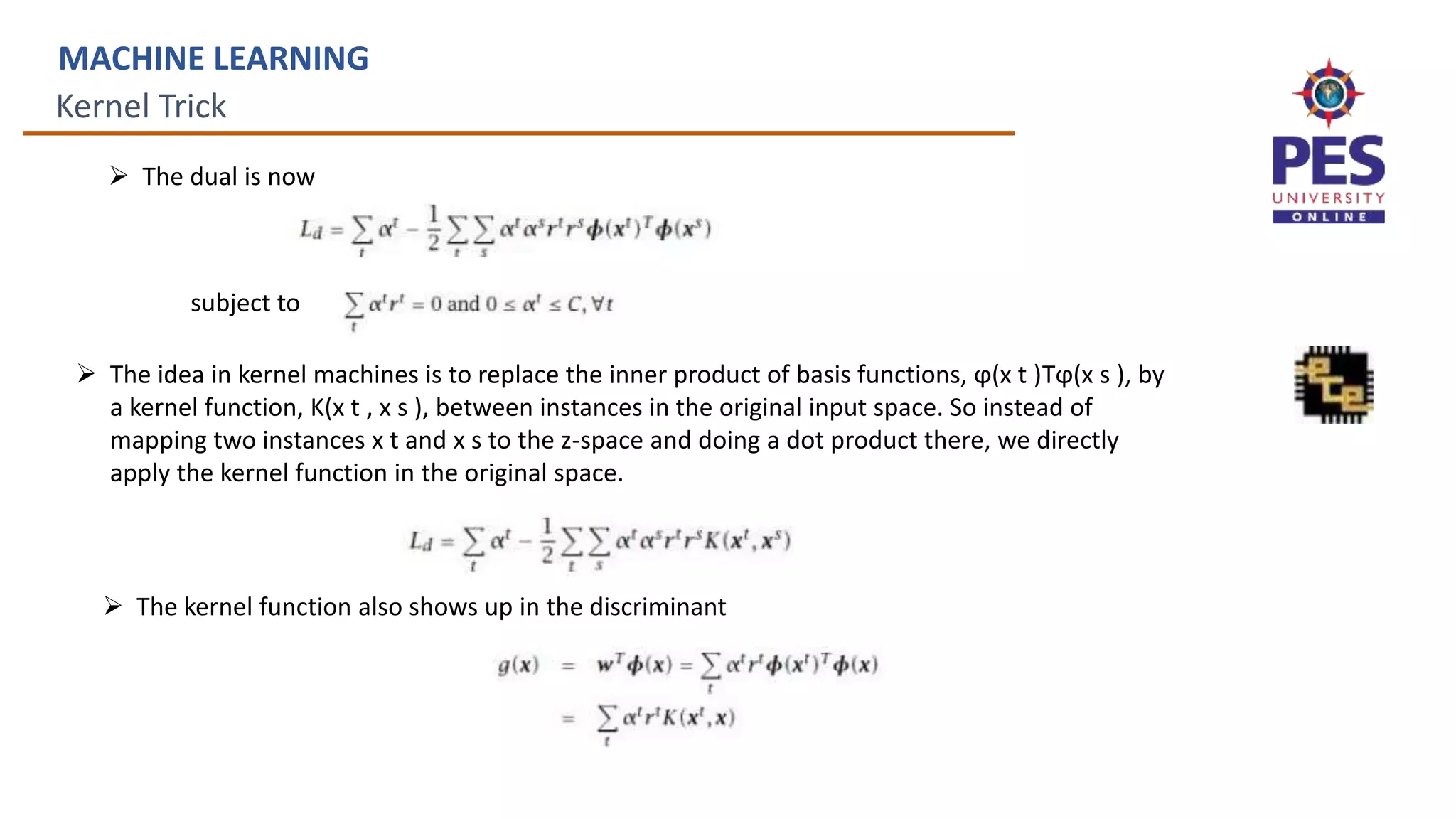
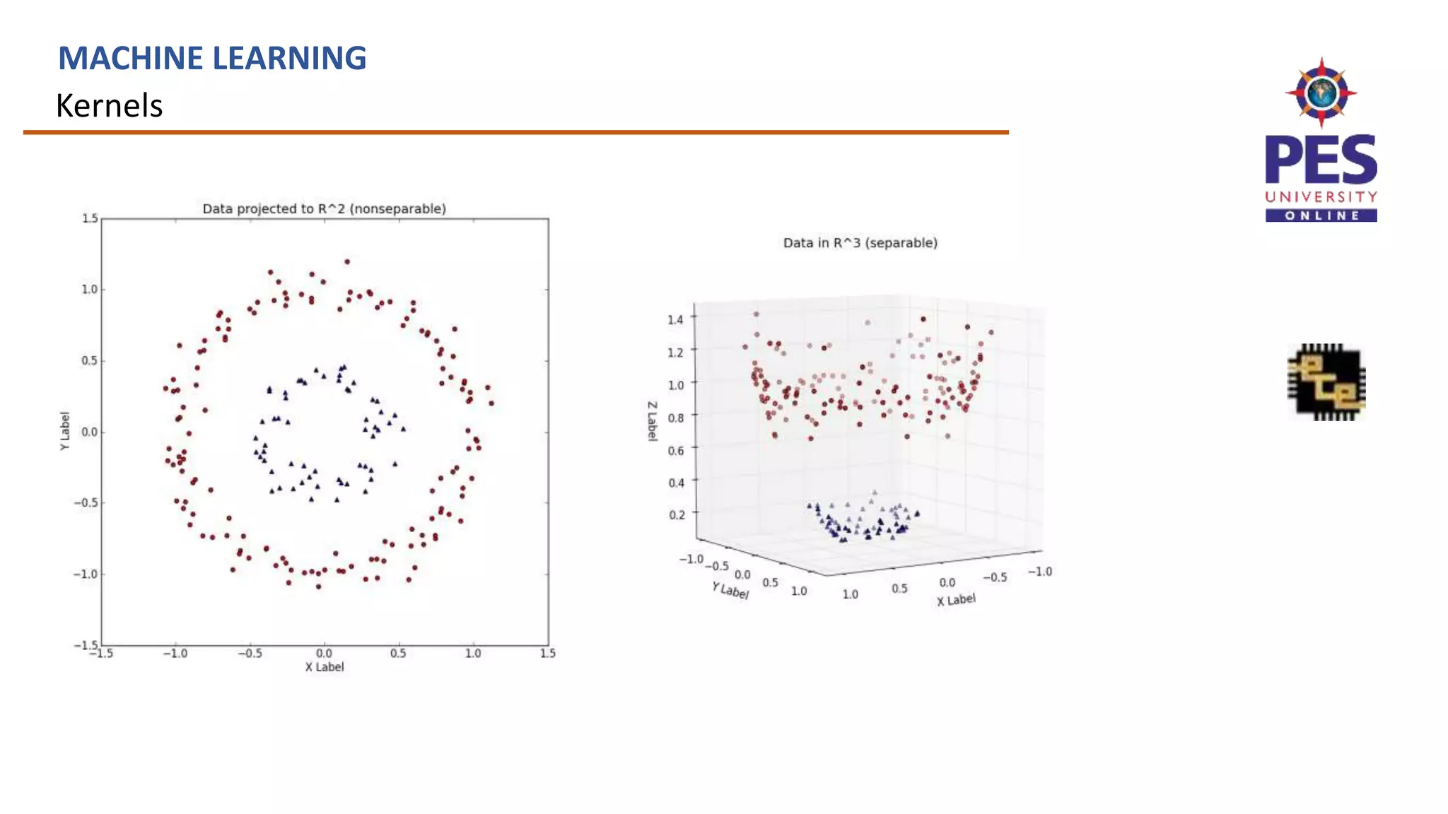
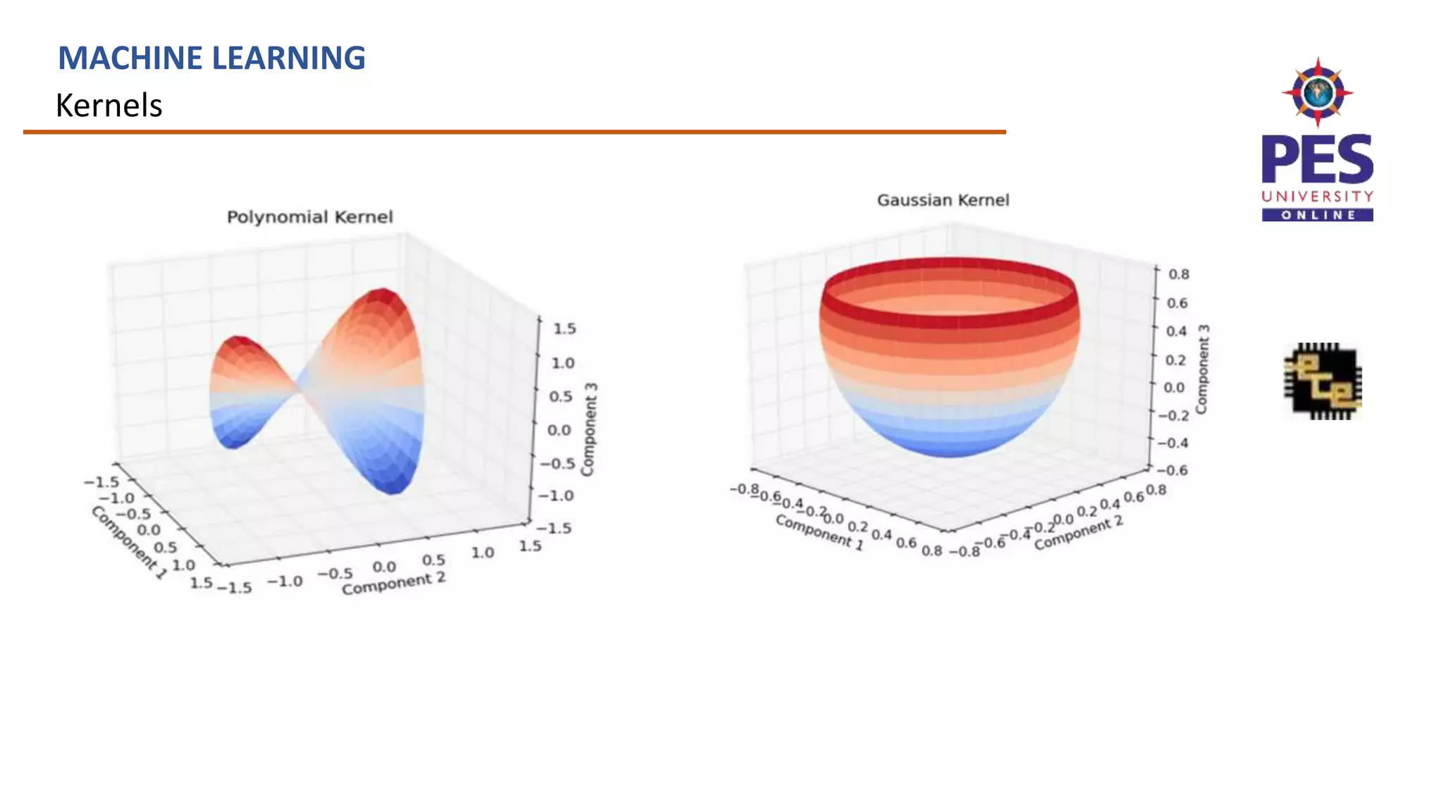
This document provides an overview of kernel machines and the kernel trick in machine learning. It discusses how the kernel trick allows projecting data into a higher dimensional space to make it linearly separable. It describes using kernels like polynomial kernels in the dual formulation to calculate dot products without explicitly performing the projection. The kernel trick avoids having to compute in the higher dimensional space, improving computational efficiency.

1. UE19EC353-Machine Learning
Kernel Machines
Veena S
Department of ECE, PESU.

2. TEXT BOOK AND REFERENCES
TEXT BOOK:
“Introduction to Machine Learning”, Ethem Alpaydin , 4th Edition, MIT Press,
2020.
REFERENCE BOOKS:
1. “Machine Learning”, Tom M. Mitchell, McGraw Hill, 1997.
2. “Pattern Recognition and Machine Learning”, Christopher M. Bishop,
Springer, 2006.
3. “Machine Learning: A Probabilistic Perspective”, Kevin P. Murphy, MIT Press,
2012.
SIGNALS & SYSTEMS

3. Text Book
Source:Introduction to
Machine Learning”, Ethem
Alpaydin , 4th Edition, MIT
Press, 2020.

4. Overview-SVM
MACHINE LEARNING
 SVM is a supervised machine learning algorithm used for both classification and regression.
 The objective of SVM algorithm algorithm is to find a hyperplane in a N dimensional space
that distinctly classifies the data points.

5. Overview-SVM
MACHINE LEARNING
SVM features:
 Discriminant-based: No need to estimate densities first
 Define the discriminant in terms of support vectors
 The use of kernel functions, application-specific measures of similarity
 No need to represent instances as vectors
 Convex optimization problems with a unique solution

6. Optimal Separating Hyperplane
MACHINE LEARNING
 
  1
as
rewritten
be
can
which
1
for
1
1
for
1
such that
and
find
if
1
if
1
where
,
0
0
0
0
2
1






















w
r
r
w
r
w
w
C
C
r
r
t
T
t
t
t
T
t
t
T
t
t
t
t
t
t
x
w
x
w
x
w
w
x
x
x
X
 Support Vector Machine is the supervised machine learning algorithm, that is used in both
classification and regression of models. The idea behind it is simple to just find a plane or a
boundary that separates the data between two classes.

7. Optimal Separating Hyperplane
MACHINE LEARNING
 Not only do we want the instances to be on the right side of the hyperplane, but we also want
them some distance away, for better generalization.
 The distance from the hyperplane to the instances closest to it on either side is called the margin,
which we want to maximize for best generalization.
 Distance from the discriminant to the closest instances on either side
 Distance of x to the hyperplane is
 We require
 For a unique sol’n, fix ρ||w||=1, and to max margin
w
x
w 0
w
t
T

  t
w
r t
T
t



,

w
x
w 0
  t
w
r t
T
t



 ,
1
2
1
0
2
x
w
w to
subject
min

8. Optimal Separating Hyperplane
MACHINE LEARNING
 In finding the optimal hyperplane, we can
convert the optimization problem to a form
whose complexity depends on N, the number
of training instances, and not on d.
 To get the new formulation, we first write
equation 14.3 as an unconstrained problem
using Lagrange multipliers α t :
 
 
 
 
0
0
0
2
1
1
2
1
,
1
subject to
2
1
min
1
0
1
1
1
0
2
1
0
2
0
2
































N
t
t
t
p
N
t
t
t
t
p
N
t
t
N
t
t
T
t
t
N
t
t
T
t
t
p
t
T
t
r
w
L
r
L
w
r
w
r
L
t
w
r





x
w
w
x
w
w
x
w
w
x
w
w

9. Optimal Separating Hyperplane
MACHINE LEARNING
 
 
 




 














t
and
to
subject t
r
r
r
r
w
r
L
t
t
t
t
t
s
T
t
s
t
t s
s
t
t
t
T
t t
t
t
t
t
t
t
t
T
T
d
,
0
0
2
1
2
1
2
1
0









x
x
w
w
x
w
w
w

10. Optimal Separating Hyperplane
MACHINE LEARNING
 which we maximize with respect to α t only, subject to the constraints
 Once we solve for α t , we see that though there are N of them, most vanish with α t = 0 and
only a small percentage have α t > 0.
 The set of x t whose α t > 0 are the support vectors, and as we see in equation
w is written as the weighted sum of these training instances that are selected as the support
vectors.
 These are the x t that satisfy
 During testing, we do not enforce a margin. We calculate g(x) = wTx + w0, and choose according
to the sign of g(x): Choose C1 if g(x) > 0 and C2 otherwise






 N
t
t
t
t
p
r
L
1
0 x
w
w


11. Soft margin: Non separable case
MACHINE LEARNING
 If the data is not linearly separable, the algorithm we discussed earlier will not work. In such a
case, if the two classes are not linearly separable such that there is no hyperplane to separate
them.
 Such a linearly not separable data can be classified using two approaches.
1. Linear SVM with soft margin
2. Non-linear SVM

12. Soft margin: Non separable case
MACHINE LEARNING
 Suppose, X1 and X2 are two instances.
 We see that the hyperplane H1 classifies wrongly both X1 and
X2.
 Also, we may note that with X1 and X2, we could draw another
hyperplane namely H2, which could classify all training data
correctly.
 However, H1 is more preferable than H2 as H1 has higher
margin compared to H2 and thus H1 is less susceptible to over
fitting.
 In other words, a linear SVM can be refitted to learn a
hyperplane that is tolerable to a small number of non-separable
training data.
 The approach of refitting is called soft margin approach (hence,
the SVM is called Soft Margin SVM), where it introduces slack
variables to the inseparable cases
This idea is based on a simple premise: allow
SVM to make a certain number of mistakes and
keep margin as wide as possible so that other
points can still be classified correctly. This can be
done simply by modifying the objective of SVM.

13. Soft margin: Non separable case
MACHINE LEARNING
 Recall that for linear SVM, we are to determine a maximum margin hyperplane W.X + b = 0 with the
following optimization:
 In soft margin SVM, we consider the similar optimization technique except that a relaxation of
inequalities, so that it also satisfies the case of linearly not separable data.
 To do this, soft margin SVM introduces slack variable (ξ), a positive-value into the constraint of
optimization problem. Thus, for soft margin we rewrite the optimization problem as follows

14. Soft margin: Non separable case
MACHINE LEARNING
 If ξ t = 0, there is no problem with x t .
 If 0 < ξ t < 1, x t is correctly classified but in
the margin.
 If ξ t ≥ 1, x t is misclassified
 The number of misclassifications is #{ξ t > 1},
 The number of nonseparable points is #{ξt >
0}. We define soft error as
 Add this as a penalty term:
Subject to
• C is the penalty factor as in any
regularization scheme trading off
complexity,

15. Soft margin: Non separable case
MACHINE LEARNING
 Here, C is a hyperparameter that decides the trade-off between maximizing the margin
and minimizing the mistakes
 When C is small, classification mistakes are given less importance and focus is more on
maximizing the margin.
 whereas when C is large, the focus is more on avoiding misclassification at the expense of
keeping the margin small.

16. Soft margin: Non separable case
MACHINE LEARNING
Adding the constraints, the Lagrangian equation becomes
 To maximize the Lagrangian equation differentiate it with W and
 we get the dual that we maximize with respect to α t :

17. Soft margin: Non separable case
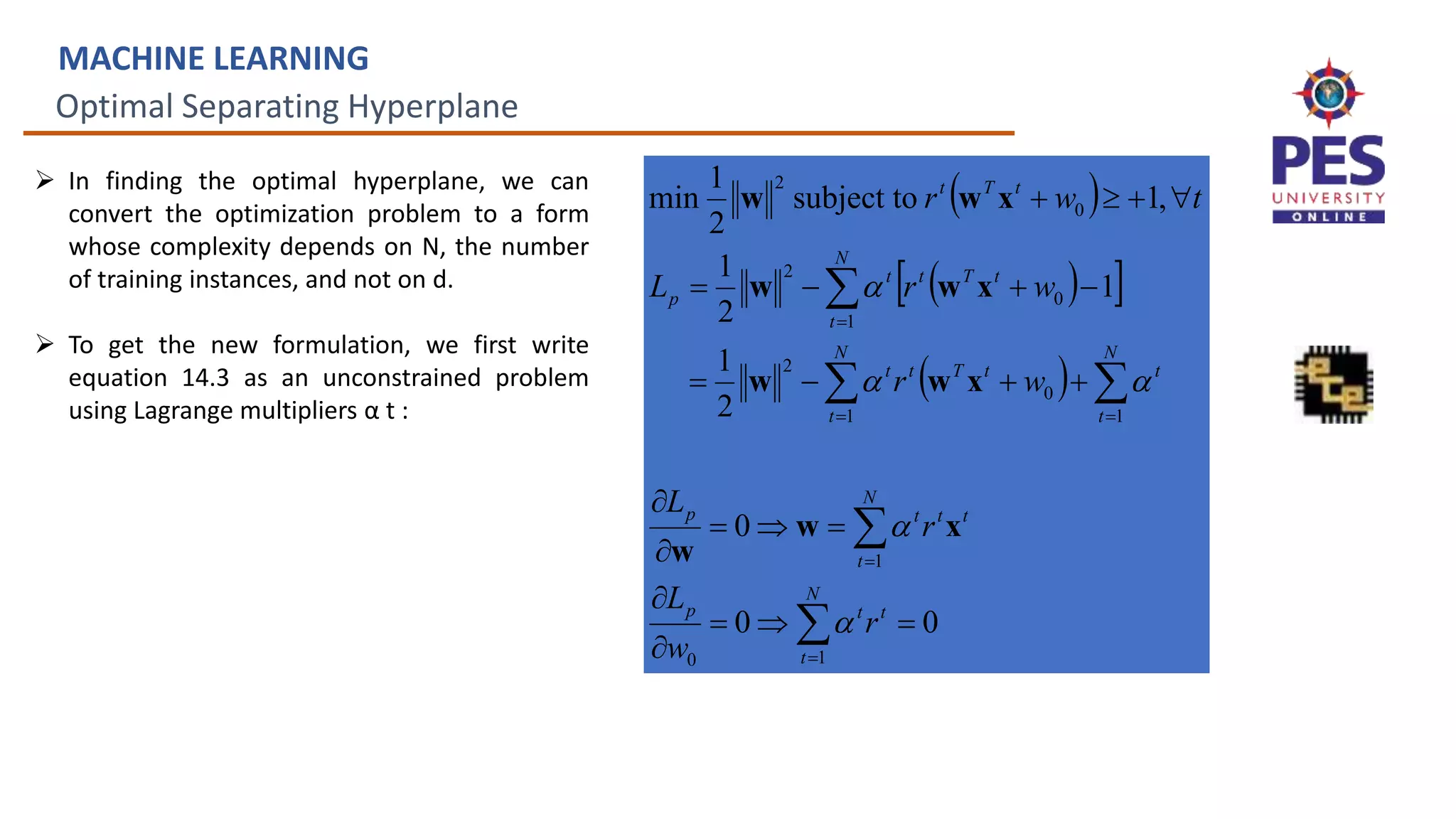
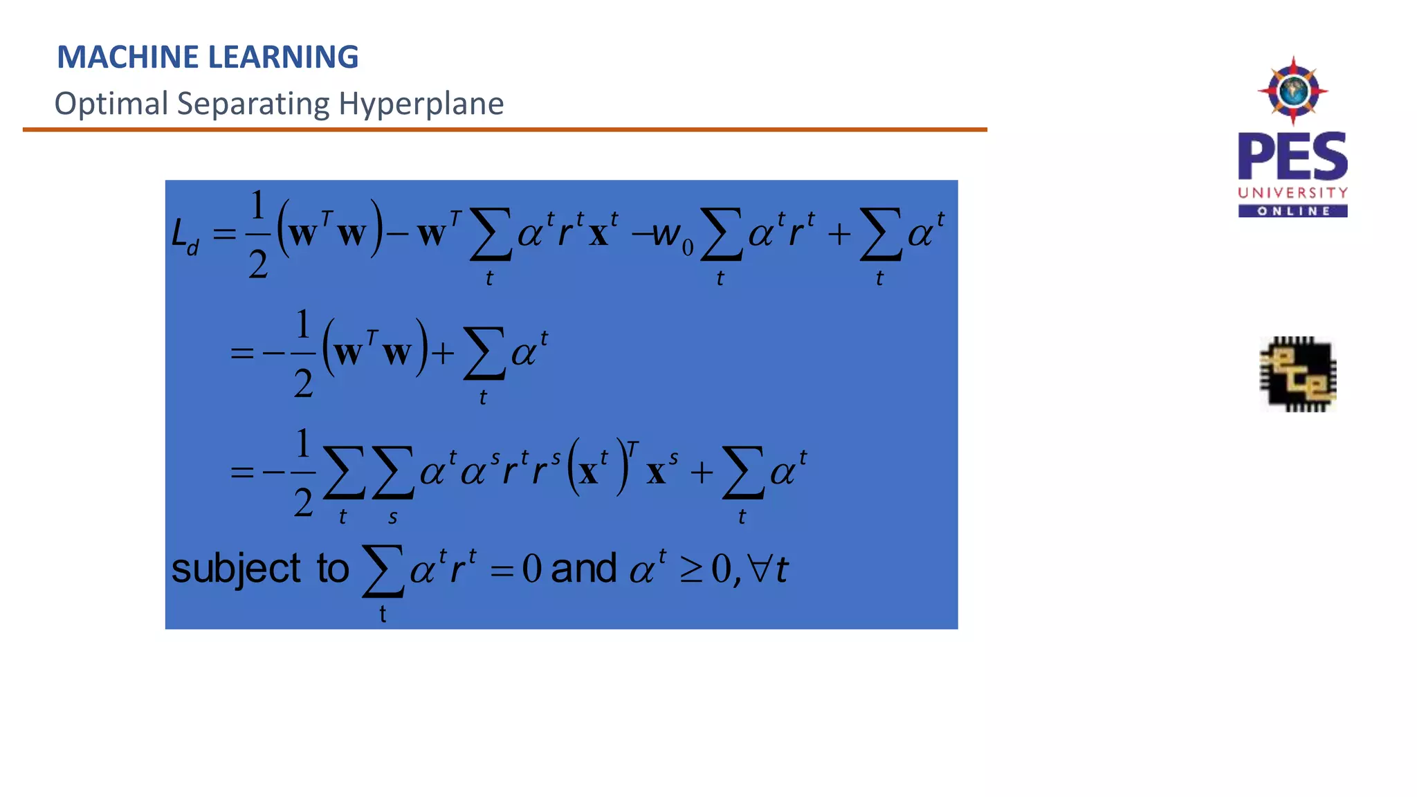
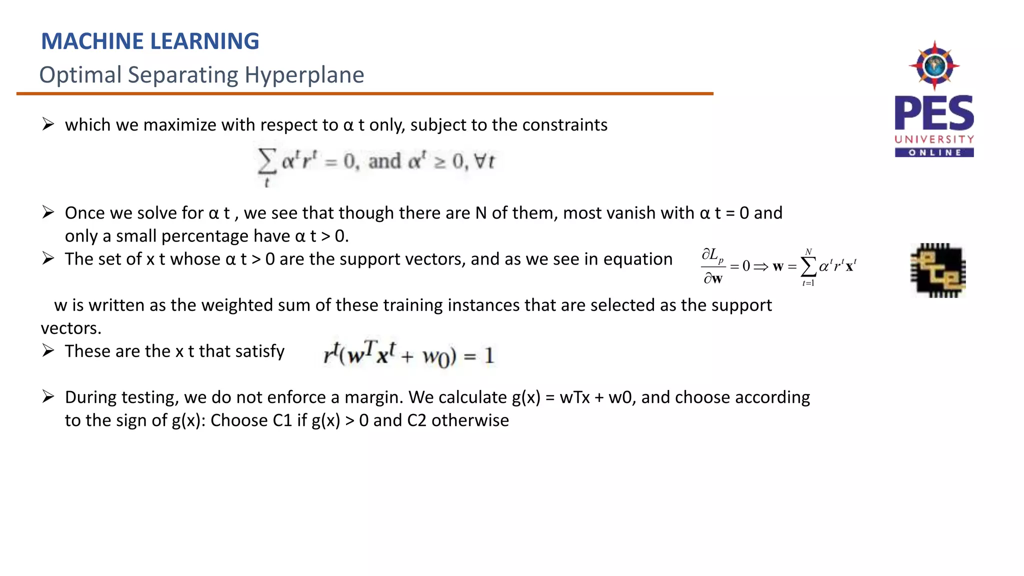
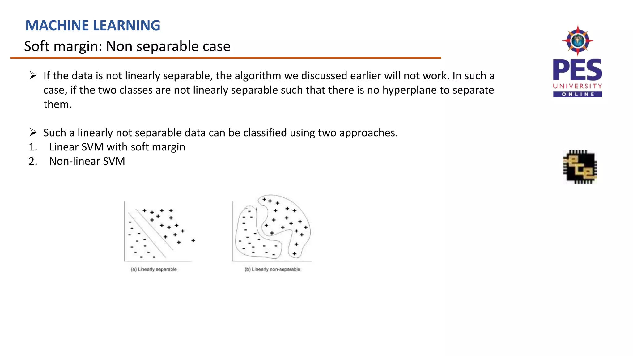
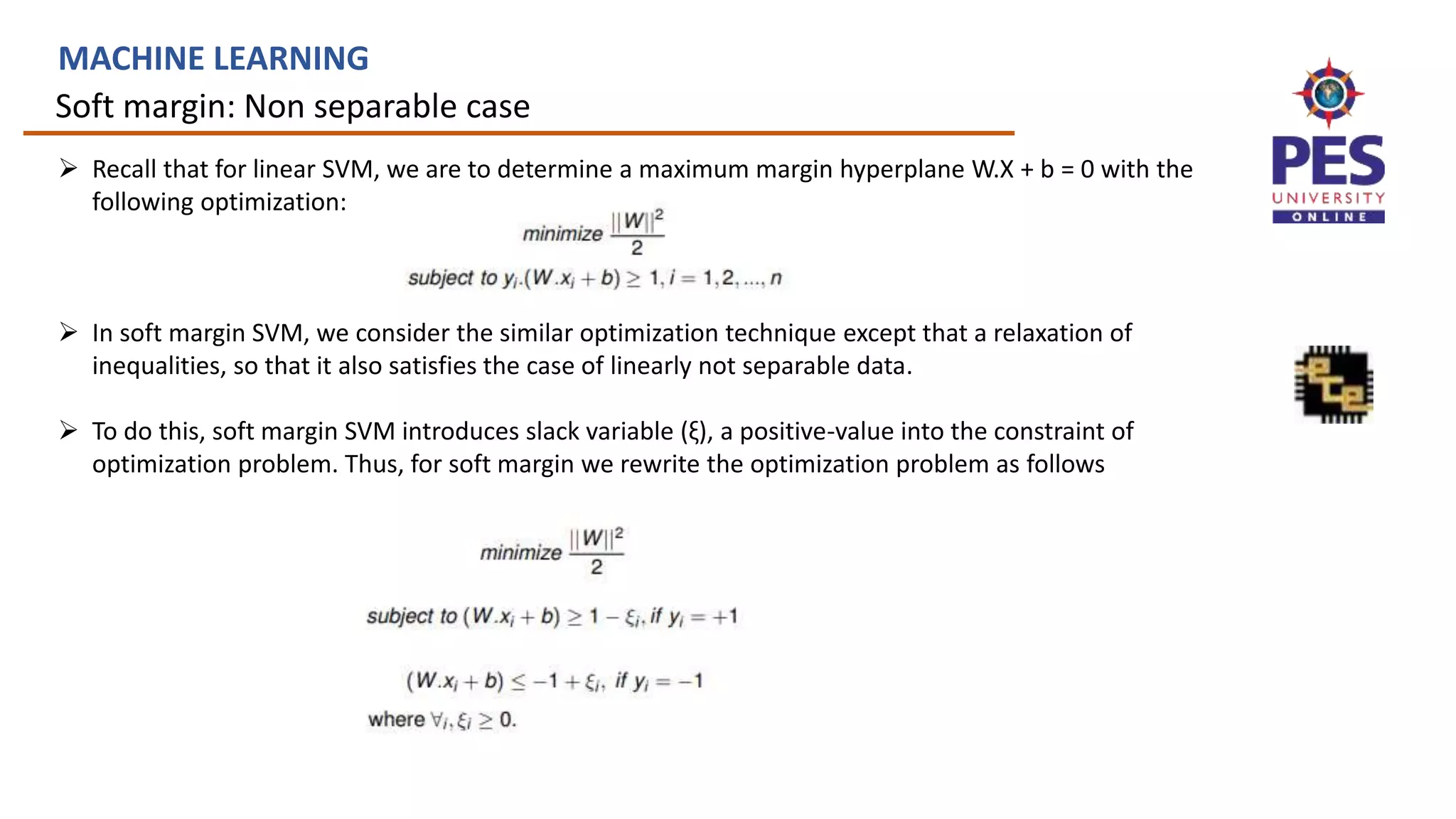
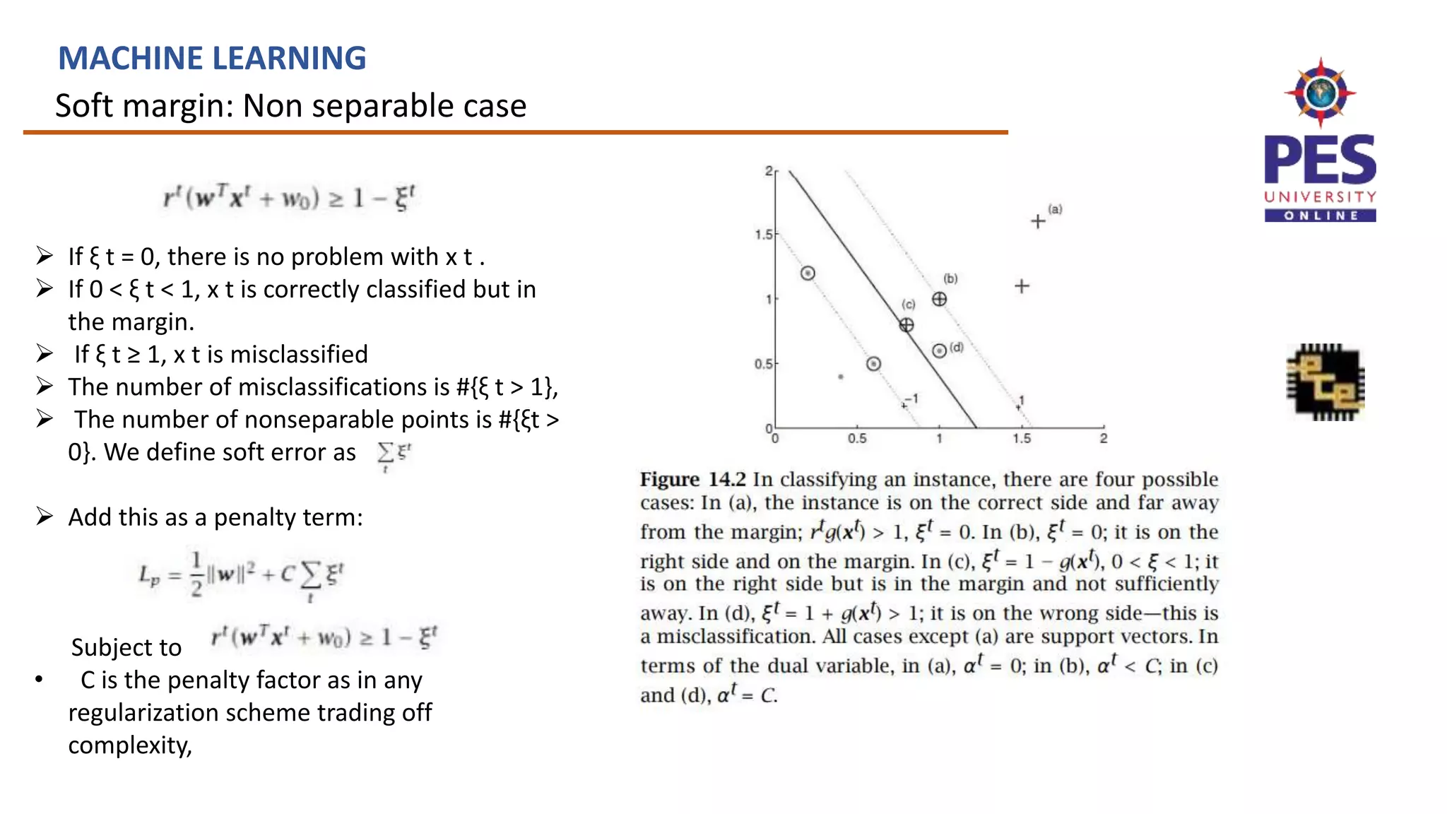
MACHINE LEARNING
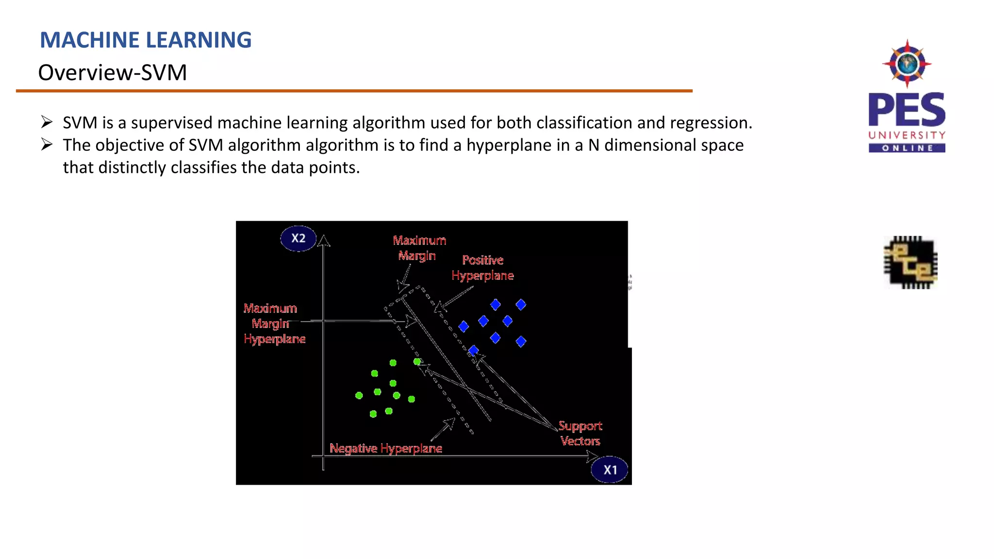
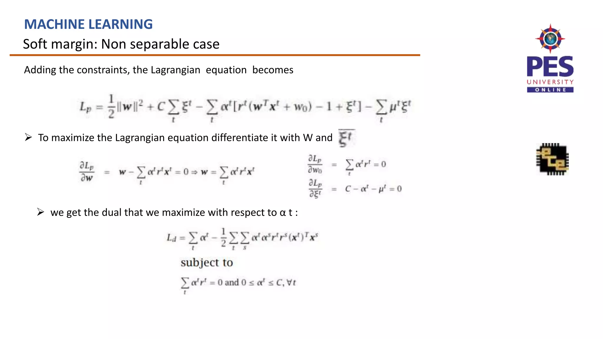
 α t = 0 implies samples are sufficiently present at larger distance and they vanish.
 α t > 0 and they define w,
• α t < C are the ones that are on the margin, they have ξ t = 0 and satisfy r t (wTx t + w0) = 1.
• α t = C instances that are in the margin or misclassified.
 The number of support vectors is an upper-bound estimate for the expected number of errors
where EN[·] denotes expectation over training sets of size N.

18. Hinge Loss
MACHINE LEARNING






otherwise
if
t
t
t
t
t
t
hinge
r
y
r
y
r
y
L
1
1
0
)
,
(
 The hinge loss is a specific type of cost function that
incorporates a margin or distance from the classification
boundary into the cost calculation. Even if new observations
are classified correctly, they can incur a penalty if the margin
from the decision boundary is not large enough.

19. n-SVM
MACHINE LEARNING
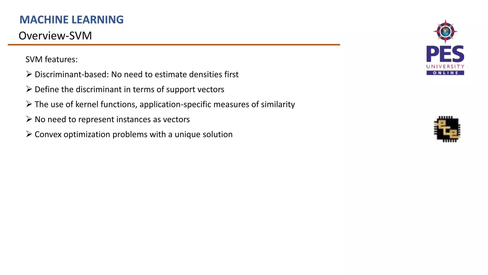
 Equivalent formulation of the soft margin hyperplane that uses a parameter ν ∈ [0, 1] instead
of C . The objective function is
 
 
n










n

















t
t
t
t
t
N
t s
s
T
t
s
t
s
t
d
t
t
t
T
t
t
t
N
r
x
x
r
r
L
ivenby
thedualisg
w
r
N
,
1
0
,
0
subject to
2
1
,
0
,
0
,
subject to
1
-
2
1
min
t
1
0
2
x
w
w • ρ is a new parameter that is a variable of the optimization
problem and scales the margin: The margin is now
2ρ/∥w∥.
• The nu parameter is both a lower bound for the number
of samples that are support vectors and an upper bound
for the number of samples that are on the wrong side of
the hyperplane.

20. Kernel Trick
MACHINE LEARNING
 A Kernel Trick is a simple method where a Non Linear data is projected onto a higher
dimension space so as to make it easier to classify the data where it could be linearly
divided by a plane.
 This is mathematically achieved by Lagrangian formula using Lagrangian multipliers.

23. Kernel Trick
MACHINE LEARNING
 Let us say we have the new dimensions calculated through the basis functions.
 mapping from the d-dimensional x space to the kdimensional z space where we write the
discriminant
 Generally, k is much larger than d and k may also be larger than N, and there lies the advantage
of using the dual form whose complexity depends on N, whereas if we used the primal it would
depend on k.

24. Kernel Trick
MACHINE LEARNING
 We also use the more general case of the soft margin hyperplane here because we have no
guarantee that the problem is linearly separable in this new space.
 The problem is the same
 constraints are defined in the new space
 The Lagrangian is

25. Kernel Trick
MACHINE LEARNING
 The dual is now
subject to
 The idea in kernel machines is to replace the inner product of basis functions, ϕ(x t )Tϕ(x s ), by
a kernel function, K(x t , x s ), between instances in the original input space. So instead of
mapping two instances x t and x s to the z-space and doing a dot product there, we directly
apply the kernel function in the original space.
 The kernel function also shows up in the discriminant

26. Kernel Trick
MACHINE LEARNING
 The matrix of kernel values, K, where Kts = K(x t , x s ), is called the Gram matrix, which should
be symmetric and positive semidefinite

27. Vectorial kernels-
MACHINE LEARNING
Polynomial Kernels
Polynomials of degree q:
   q
t
T
t
K 1

 x
x
x
x ,
   
 
   T
T
x
x
x
x
x
x
y
x
y
x
y
y
x
x
y
x
y
x
y
x
y
x
K
2
2
2
1
2
1
2
1
2
2
2
2
2
1
2
1
2
1
2
1
2
2
1
1
2
2
2
1
1
2
2
2
2
1
2
2
2
1
1
1
,
,
,
,
,
,












x
y
x
y
x

Polynomial Kernels

28. RBF (Gaussian) Kernel
MACHINE LEARNING
Radial-basis functions:
 







 

 2
2
2s
K
t
t
x
x
x
x exp
,
 The boundary and margins found by the
Gaussian kernel with different spread
values, s2. We get smoother boundaries
with larger spreads.
 The best value of variance is found by
cross validation.

29. RBF (Gaussian) Kernel
MACHINE LEARNING
 We can have a Mahalanobis kernel, generalizing from the Euclidean distance:
 where S is a covariance matrix. Or, in the most general case,
 sigmoidal functions:

30. Kernels
MACHINE LEARNING

31. Kernels
MACHINE LEARNING

32. Kernels
MACHINE LEARNING

33. Defining Kernels
MACHINE LEARNING
 Kernels are generally considered to be measures of similarity in the sense that K(x,
y) takes a larger value as x and y are more “similar,” from the point of view of the
application.
 Prior knowledge we have regarding the application can be provided to the learner
through appropriately defined kernels.
 We have string kernels, tree kernels, graph kernels, and so on depending on how
we represent the data and how we measure similarity in that representation

34. Defining Kernels-Bag of words
MACHINE LEARNING
 BoW-A method of feature extraction with text data. This approach is a simple and flexible
way of extracting features from documents.
 A bag of words is a representation of text that describes the occurrence of words within a
document. We just keep track of word counts and disregard the grammatical details and
the word order.
 The model is only concerned with whether known words occur in the document, not
where in the document.
 Let us say D1 and D2 are two documents and one possible representation is called bag of
words .
 we predefine M words relevant for the application, and we define ϕ(D1) as the M-
dimensional binary vector
I. 1 if word appears in D1
II. is 0 otherwise.
 Then, ϕ(D1)T ϕ(D2) counts the number of shared words.

35. Defining kernels
MACHINE LEARNING
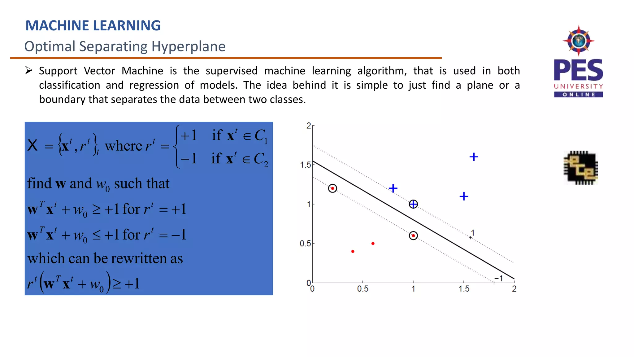
 Empirical kernel map: Define a set of templates mi and score function
s(x,mi)
f(xt)=[s(xt,m1), s(xt,m2),..., s(xt,mM)]
and
K(x,xt)=f (x)T f (xt)
 Fisher Kernel-is a function that measures the similarity of two objects on
the basis of sets of measurements for each object and a statistical model.

36. Multiple Kernel Learning
MACHINE LEARNING
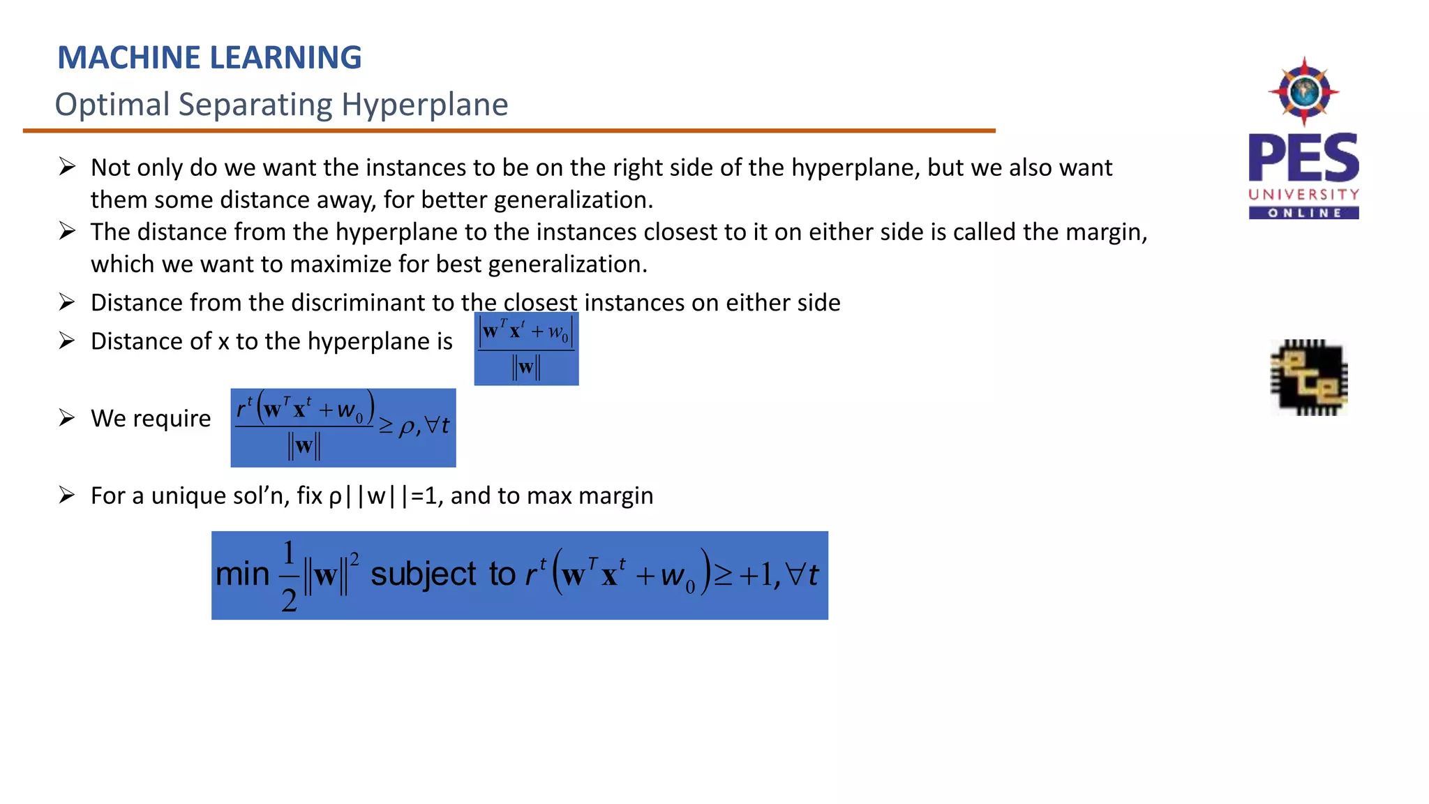
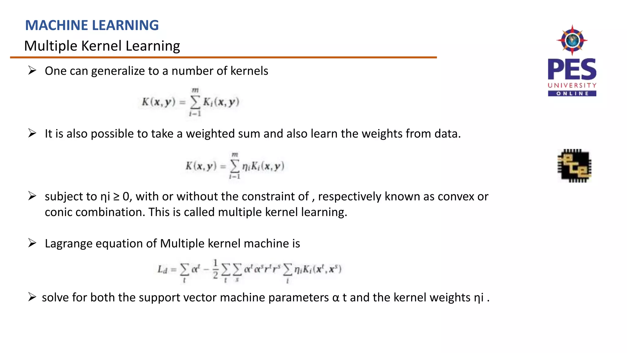
 It is possible to construct new kernels by combining simpler kernels. If K1(x, y)
and K2(x, y) are valid kernels and c a constant.
 Fixed kernel combination:
 Adaptive kernel combination:
 Where
 
 
   
   







y
x
y
x
y
x
y
x
y
x
y
x
,
,
,
,
,
,
2
1
2
1
K
K
K
K
cK
K
x = [xA, xB]

37. Multiple Kernel Learning
MACHINE LEARNING
 One can generalize to a number of kernels
 It is also possible to take a weighted sum and also learn the weights from data.
 subject to ηi ≥ 0, with or without the constraint of , respectively known as convex or
conic combination. This is called multiple kernel learning.
 Lagrange equation of Multiple kernel machine is
 solve for both the support vector machine parameters α t and the kernel weights ηi .

38. Multiple Kernel Learning
MACHINE LEARNING
 Discriminant function is given by
 After training, ηi will take values depending on how the corresponding kernel Ki (x t , x) is
useful in discriminating.
 Localised Kernel Combination:

39. Multiclass Kernel Machines
MACHINE LEARNING
 1-vs-all
• each one separating one class from all other classes combined and learn K support
vector machines gi (x), i = 1, … , K

40. Multiclass Kernel Machines
MACHINE LEARNING

41. Multiclass Kernel Machines
MACHINE LEARNING

42. Multiclass Kernel Machines
MACHINE LEARNING

43. Multiple Kernel Learning
MACHINE LEARNING

44. Overview
MACHINE LEARNING

45. THANK YOU
Veena S
Department of ECE