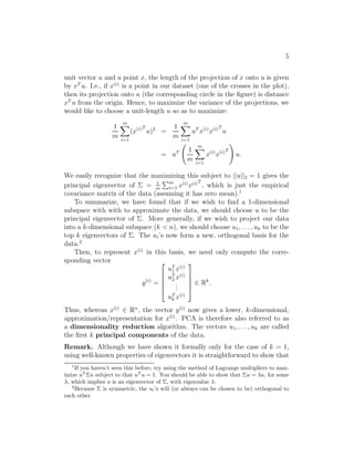
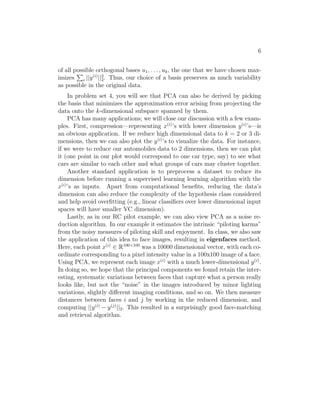
CS229 Lecture notes 
Andrew Ng 
Part XI 
Principal components analysis 
In our discussion of factor analysis, we gave a way to model data x ∈ Rn as 
“approximately” lying in some k-dimension subspace, where k ≪ n. Specif- 
ically, we imagined that each point x(i) was created by first generating some 
z(i) lying in the k-dimension affine space {z + μ; z ∈ Rk}, and then adding 
	-covariance noise. Factor analysis is based on a probabilistic model, and 
parameter estimation used the iterative EM algorithm. 
In this set of notes, we will develop a method, Principal Components 
Analysis (PCA), that also tries to identify the subspace in which the data 
approximately lies. However, PCA will do so more directly, and will require 
only an eigenvector calculation (easily done with the eig function in Matlab), 
and does not need to resort to EM. 
Suppose we are given a dataset {x(i); i = 1, . . . ,m} of attributes of m dif- 
ferent types of automobiles, such as their maximum speed, turn radius, and 
so on. Let x(i) ∈ Rn for each i (n ≪ m). But unknown to us, two different 
attributes—some xi and xj—respectively give a car’s maximum speed mea- 
sured in miles per hour, and the maximum speed measured in kilometers per 
hour. These two attributes are therefore almost linearly dependent, up to 
only small differences introduced by rounding off to the nearest mph or kph. 
Thus, the data really lies approximately on an n − 1 dimensional subspace. 
How can we automatically detect, and perhaps remove, this redundancy? 
For a less contrived example, consider a dataset resulting from a survey of 
pilots for radio-controlled helicopters, where x(i) 
1 is a measure of the piloting 
skill of pilot i, and x(i) 
2 captures how much he/she enjoys flying. Because 
RC helicopters are very difficult to fly, only the most committed students, 
ones that truly enjoy flying, become good pilots. So, the two attributes 
x1 and x2 are strongly correlated. Indeed, we might posit that that the 
1
2 
data actually likes along some diagonal axis (the u1 direction) capturing the 
intrinsic piloting “karma” of a person, with only a small amount of noise 
lying off this axis. (See figure.) How can we automatically compute this u1 
direction? 
x1 
x2 (enjoyment) 
(skill) 
1 
u 
u 
2 
We will shortly develop the PCA algorithm. But prior to running PCA 
per se, typically we first pre-process the data to normalize its mean and 
variance, as follows: 
1. Let μ = 1 
m 
Pm 
i=1 x(i). 
2. Replace each x(i) with x(i) − μ. 
j = 1 
3. Let 2 
m 
P 
i(x(i) 
j )2 
4. Replace each x(i) 
j with x(i) 
j /j . 
Steps (1-2) zero out the mean of the data, and may be omitted for data 
known to have zero mean (for instance, time series corresponding to speech 
or other acoustic signals). Steps (3-4) rescale each coordinate to have unit 
variance, which ensures that different attributes are all treated on the same 
“scale.” For instance, if x1 was cars’ maximum speed in mph (taking values 
in the high tens or low hundreds) and x2 were the number of seats (taking 
values around 2-4), then this renormalization rescales the different attributes 
to make them more comparable. Steps (3-4) may be omitted if we had 
apriori knowledge that the different attributes are all on the same scale. One
3 
example of this is if each data point represented a grayscale image, and each 
x(i) 
j took a value in {0, 1, . . . , 255} corresponding to the intensity value of 
pixel j in image i. 
Now, having carried out the normalization, how do we compute the “ma- 
jor axis of variation” u—that is, the direction on which the data approxi- 
mately lies? One way to pose this problem is as finding the unit vector u so 
that when the data is projected onto the direction corresponding to u, the 
variance of the projected data is maximized. Intuitively, the data starts off 
with some amount of variance/information in it. We would like to choose a 
direction u so that if we were to approximate the data as lying in the direc- 
tion/subspace corresponding to u, as much as possible of this variance is still 
retained. 
Consider the following dataset, on which we have already carried out the 
normalization steps: 
Now, suppose we pick u to correspond the the direction shown in the 
figure below. The circles denote the projections of the original data onto this 
line.
4 


We see that the projected data still has a fairly large variance, and the 
points tend to be far from zero. In contrast, suppose had instead picked the 
following direction: 


Here, the projections have a significantly smaller variance, and are much 
closer to the origin. 
We would like to automatically select the direction u corresponding to 
the first of the two figures shown above. To formalize this, note that given a
5 
unit vector u and a point x, the length of the projection of x onto u is given 
by xT u. I.e., if x(i) is a point in our dataset (one of the crosses in the plot), 
then its projection onto u (the corresponding circle in the figure) is distance 
xT u from the origin. Hence, to maximize the variance of the projections, we 
would like to choose a unit-length u so as to maximize: 
1 
m 
Xm 
i=1 
(x(i)T 
u)2 = 
1 
m 
Xm 
i=1 
uTx(i)x(i)T 
u 
= uT 
  
1 
m 
Xm 
i=1 
x(i)x(i)T 
! 
u. 
We easily recognize that the maximizing this subject to ||u||2 = 1 gives the 
principal eigenvector of  = 1 
m 
Pm 
i=1 x(i)x(i)T 
, which is just the empirical 
covariance matrix of the data (assuming it has zero mean).1 
To summarize, we have found that if we wish to find a 1-dimensional 
subspace with with to approximate the data, we should choose u to be the 
principal eigenvector of . More generally, if we wish to project our data 
into a k-dimensional subspace (k  n), we should choose u1, . . . , uk to be the 
top k eigenvectors of . The ui’s now form a new, orthogonal basis for the 
data.2 
Then, to represent x(i) in this basis, we need only compute the corre- 
sponding vector 
y(i) = 
 
 
uT1 
x(i) 
uT2 
x(i) 
... 
uT 
k x(i) 
 
 
∈ Rk. 
Thus, whereas x(i) ∈ Rn, the vector y(i) now gives a lower, k-dimensional, 
approximation/representation for x(i). PCA is therefore also referred to as 
a dimensionality reduction algorithm. The vectors u1, . . . , uk are called 
the first k principal components of the data. 
Remark. Although we have shown it formally only for the case of k = 1, 
using well-known properties of eigenvectors it is straightforward to show that 
1If you haven’t seen this before, try using the method of Lagrange multipliers to max- 
imize uTu subject to that uT u = 1. You should be able to show that u = u, for some 
, which implies u is an eigenvector of , with eigenvalue . 
2Because  is symmetric, the ui’s will (or always can be chosen to be) orthogonal to 
each other.
6 
of all possible P 
orthogonal bases u1, . . . , uk, the one that we have chosen max- 
imizes 
i ||y(i)||22 
. Thus, our choice of a basis preserves as much variability 
as possible in the original data. 
In problem set 4, you will see that PCA can also be derived by picking 
the basis that minimizes the approximation error arising from projecting the 
data onto the k-dimensional subspace spanned by them. 
PCA has many applications; we will close our discussion with a few exam- 
ples. First, compression—representing x(i)’s with lower dimension y(i)’s—is 
an obvious application. If we reduce high dimensional data to k = 2 or 3 di- 
mensions, then we can also plot the y(i)’s to visualize the data. For instance, 
if we were to reduce our automobiles data to 2 dimensions, then we can plot 
it (one point in our plot would correspond to one car type, say) to see what 
cars are similar to each other and what groups of cars may cluster together. 
Another standard application is to preprocess a dataset to reduce its 
dimension before running a supervised learning learning algorithm with the 
x(i)’s as inputs. Apart from computational benefits, reducing the data’s 
dimension can also reduce the complexity of the hypothesis class considered 
and help avoid overfitting (e.g., linear classifiers over lower dimensional input 
spaces will have smaller VC dimension). 
Lastly, as in our RC pilot example, we can also view PCA as a noise re- 
duction algorithm. In our example it estimates the intrinsic “piloting karma” 
from the noisy measures of piloting skill and enjoyment. In class, we also saw 
the application of this idea to face images, resulting in eigenfaces method. 
Here, each point x(i) ∈ R100×100 was a 10000 dimensional vector, with each co- 
ordinate corresponding to a pixel intensity value in a 100x100 image of a face. 
Using PCA, we represent each image x(i) with a much lower-dimensional y(i). 
In doing so, we hope that the principal components we found retain the inter- 
esting, systematic variations between faces that capture what a person really 
looks like, but not the “noise” in the images introduced by minor lighting 
variations, slightly different imaging conditions, and so on. We then measure 
distances between faces i and j by working in the reduced dimension, and 
computing ||y(i) − y(j)||2. This resulted in a surprisingly good face-matching 
and retrieval algorithm.

Machine learning (11)

  • 1.
    CS229 Lecture notes Andrew Ng Part XI Principal components analysis In our discussion of factor analysis, we gave a way to model data x ∈ Rn as “approximately” lying in some k-dimension subspace, where k ≪ n. Specif- ically, we imagined that each point x(i) was created by first generating some z(i) lying in the k-dimension affine space {z + μ; z ∈ Rk}, and then adding -covariance noise. Factor analysis is based on a probabilistic model, and parameter estimation used the iterative EM algorithm. In this set of notes, we will develop a method, Principal Components Analysis (PCA), that also tries to identify the subspace in which the data approximately lies. However, PCA will do so more directly, and will require only an eigenvector calculation (easily done with the eig function in Matlab), and does not need to resort to EM. Suppose we are given a dataset {x(i); i = 1, . . . ,m} of attributes of m dif- ferent types of automobiles, such as their maximum speed, turn radius, and so on. Let x(i) ∈ Rn for each i (n ≪ m). But unknown to us, two different attributes—some xi and xj—respectively give a car’s maximum speed mea- sured in miles per hour, and the maximum speed measured in kilometers per hour. These two attributes are therefore almost linearly dependent, up to only small differences introduced by rounding off to the nearest mph or kph. Thus, the data really lies approximately on an n − 1 dimensional subspace. How can we automatically detect, and perhaps remove, this redundancy? For a less contrived example, consider a dataset resulting from a survey of pilots for radio-controlled helicopters, where x(i) 1 is a measure of the piloting skill of pilot i, and x(i) 2 captures how much he/she enjoys flying. Because RC helicopters are very difficult to fly, only the most committed students, ones that truly enjoy flying, become good pilots. So, the two attributes x1 and x2 are strongly correlated. Indeed, we might posit that that the 1
  • 2.
    2 data actuallylikes along some diagonal axis (the u1 direction) capturing the intrinsic piloting “karma” of a person, with only a small amount of noise lying off this axis. (See figure.) How can we automatically compute this u1 direction? x1 x2 (enjoyment) (skill) 1 u u 2 We will shortly develop the PCA algorithm. But prior to running PCA per se, typically we first pre-process the data to normalize its mean and variance, as follows: 1. Let μ = 1 m Pm i=1 x(i). 2. Replace each x(i) with x(i) − μ. j = 1 3. Let 2 m P i(x(i) j )2 4. Replace each x(i) j with x(i) j /j . Steps (1-2) zero out the mean of the data, and may be omitted for data known to have zero mean (for instance, time series corresponding to speech or other acoustic signals). Steps (3-4) rescale each coordinate to have unit variance, which ensures that different attributes are all treated on the same “scale.” For instance, if x1 was cars’ maximum speed in mph (taking values in the high tens or low hundreds) and x2 were the number of seats (taking values around 2-4), then this renormalization rescales the different attributes to make them more comparable. Steps (3-4) may be omitted if we had apriori knowledge that the different attributes are all on the same scale. One
  • 3.
    3 example ofthis is if each data point represented a grayscale image, and each x(i) j took a value in {0, 1, . . . , 255} corresponding to the intensity value of pixel j in image i. Now, having carried out the normalization, how do we compute the “ma- jor axis of variation” u—that is, the direction on which the data approxi- mately lies? One way to pose this problem is as finding the unit vector u so that when the data is projected onto the direction corresponding to u, the variance of the projected data is maximized. Intuitively, the data starts off with some amount of variance/information in it. We would like to choose a direction u so that if we were to approximate the data as lying in the direc- tion/subspace corresponding to u, as much as possible of this variance is still retained. Consider the following dataset, on which we have already carried out the normalization steps: Now, suppose we pick u to correspond the the direction shown in the figure below. The circles denote the projections of the original data onto this line.
  • 4.
    4 We see that the projected data still has a fairly large variance, and the points tend to be far from zero. In contrast, suppose had instead picked the following direction: Here, the projections have a significantly smaller variance, and are much closer to the origin. We would like to automatically select the direction u corresponding to the first of the two figures shown above. To formalize this, note that given a
  • 5.
    5 unit vectoru and a point x, the length of the projection of x onto u is given by xT u. I.e., if x(i) is a point in our dataset (one of the crosses in the plot), then its projection onto u (the corresponding circle in the figure) is distance xT u from the origin. Hence, to maximize the variance of the projections, we would like to choose a unit-length u so as to maximize: 1 m Xm i=1 (x(i)T u)2 = 1 m Xm i=1 uTx(i)x(i)T u = uT 1 m Xm i=1 x(i)x(i)T ! u. We easily recognize that the maximizing this subject to ||u||2 = 1 gives the principal eigenvector of = 1 m Pm i=1 x(i)x(i)T , which is just the empirical covariance matrix of the data (assuming it has zero mean).1 To summarize, we have found that if we wish to find a 1-dimensional subspace with with to approximate the data, we should choose u to be the principal eigenvector of . More generally, if we wish to project our data into a k-dimensional subspace (k n), we should choose u1, . . . , uk to be the top k eigenvectors of . The ui’s now form a new, orthogonal basis for the data.2 Then, to represent x(i) in this basis, we need only compute the corre- sponding vector y(i) =   uT1 x(i) uT2 x(i) ... uT k x(i)   ∈ Rk. Thus, whereas x(i) ∈ Rn, the vector y(i) now gives a lower, k-dimensional, approximation/representation for x(i). PCA is therefore also referred to as a dimensionality reduction algorithm. The vectors u1, . . . , uk are called the first k principal components of the data. Remark. Although we have shown it formally only for the case of k = 1, using well-known properties of eigenvectors it is straightforward to show that 1If you haven’t seen this before, try using the method of Lagrange multipliers to max- imize uTu subject to that uT u = 1. You should be able to show that u = u, for some , which implies u is an eigenvector of , with eigenvalue . 2Because is symmetric, the ui’s will (or always can be chosen to be) orthogonal to each other.
  • 6.
    6 of allpossible P orthogonal bases u1, . . . , uk, the one that we have chosen max- imizes i ||y(i)||22 . Thus, our choice of a basis preserves as much variability as possible in the original data. In problem set 4, you will see that PCA can also be derived by picking the basis that minimizes the approximation error arising from projecting the data onto the k-dimensional subspace spanned by them. PCA has many applications; we will close our discussion with a few exam- ples. First, compression—representing x(i)’s with lower dimension y(i)’s—is an obvious application. If we reduce high dimensional data to k = 2 or 3 di- mensions, then we can also plot the y(i)’s to visualize the data. For instance, if we were to reduce our automobiles data to 2 dimensions, then we can plot it (one point in our plot would correspond to one car type, say) to see what cars are similar to each other and what groups of cars may cluster together. Another standard application is to preprocess a dataset to reduce its dimension before running a supervised learning learning algorithm with the x(i)’s as inputs. Apart from computational benefits, reducing the data’s dimension can also reduce the complexity of the hypothesis class considered and help avoid overfitting (e.g., linear classifiers over lower dimensional input spaces will have smaller VC dimension). Lastly, as in our RC pilot example, we can also view PCA as a noise re- duction algorithm. In our example it estimates the intrinsic “piloting karma” from the noisy measures of piloting skill and enjoyment. In class, we also saw the application of this idea to face images, resulting in eigenfaces method. Here, each point x(i) ∈ R100×100 was a 10000 dimensional vector, with each co- ordinate corresponding to a pixel intensity value in a 100x100 image of a face. Using PCA, we represent each image x(i) with a much lower-dimensional y(i). In doing so, we hope that the principal components we found retain the inter- esting, systematic variations between faces that capture what a person really looks like, but not the “noise” in the images introduced by minor lighting variations, slightly different imaging conditions, and so on. We then measure distances between faces i and j by working in the reduced dimension, and computing ||y(i) − y(j)||2. This resulted in a surprisingly good face-matching and retrieval algorithm.