This document discusses image restoration and segmentation. Image restoration deals with improving degraded images by removing noise and blurring. Various noise models and filters for restoration are described, including mean filters, order statistics filters, adaptive filters, and frequency domain filters. Segmentation involves separating an image into regions or objects. Methods described include edge detection, region-based segmentation, and morphological operations like erosion and dilation.

1. UNIT -III
IMAGE RESTORATION AND SEGMENTATION
IMAGE RESTORATION :Noise models – Mean Filters –
Order Statistics – Adaptive filters – Band reject Filters –
Band pass Filters – Notch Filters – Optimum Notch
Filtering – Inverse Filtering–Wiener filtering.
SEGMENTATION: Detection of Discontinuities–Edge
Linking and Boundary detection – Region based
segmentation- Morphological processing- erosion and
dilation.
05.08.2023 KNCET 1

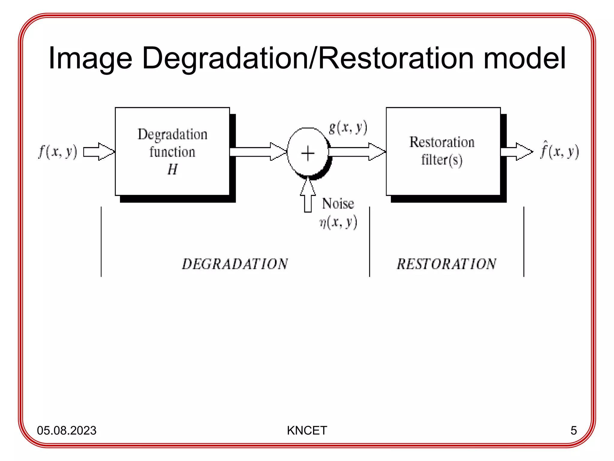
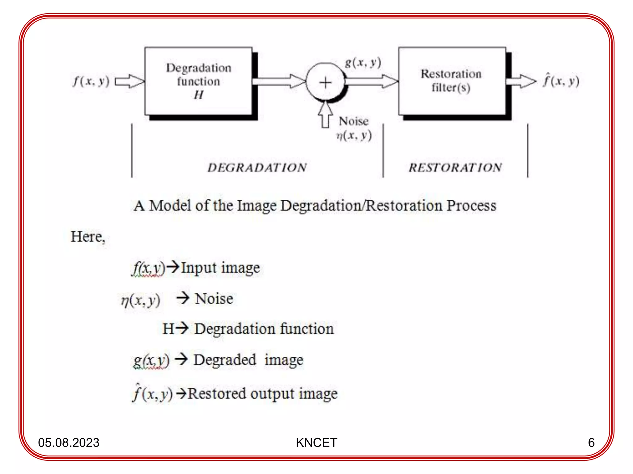
2. Image Restoration
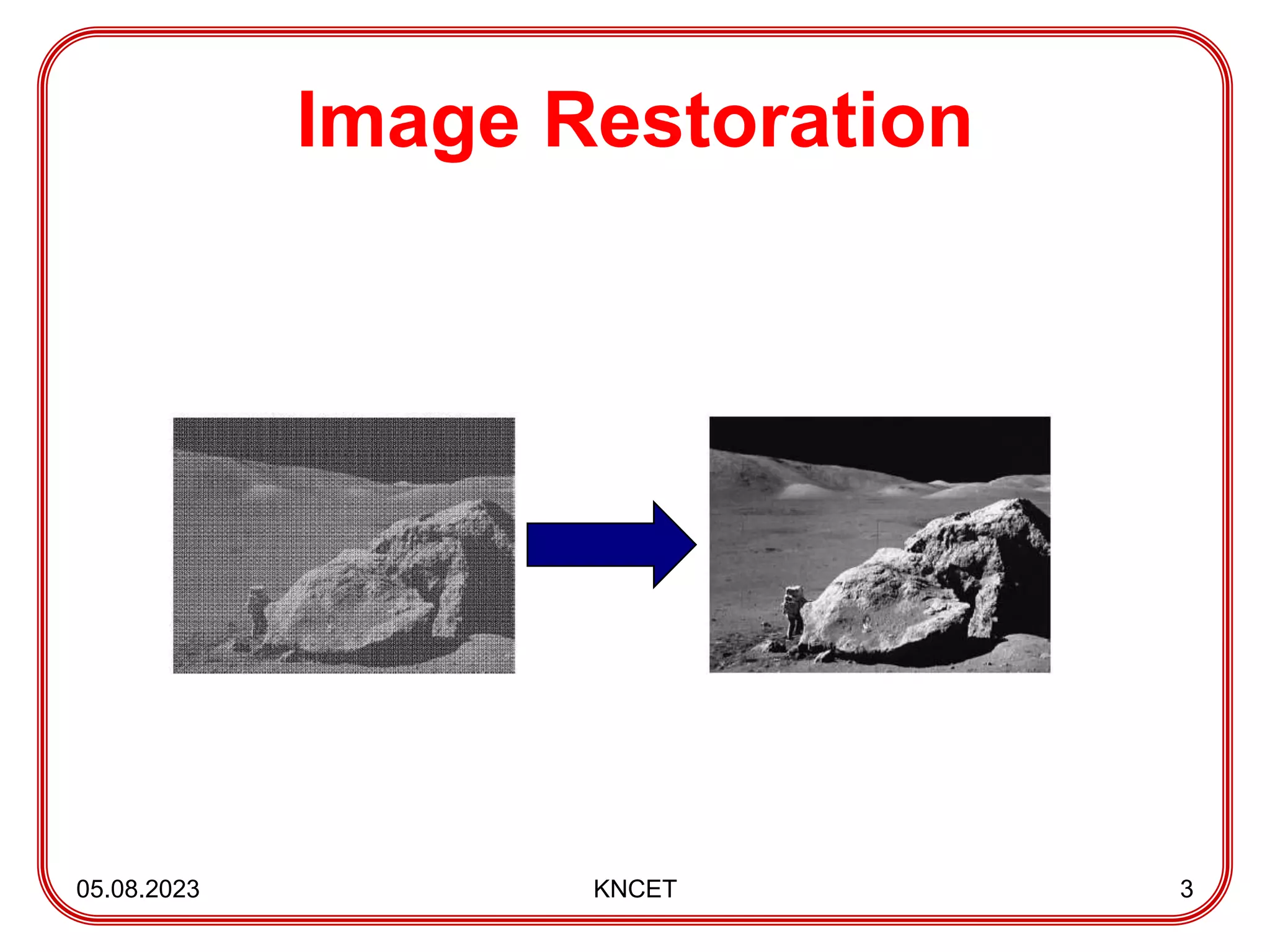
• It deals with improving the appearance of
an image.
• Restoration is a process that reconstructs
or recovers an image that has been
degraded by using a prior knowledge of
the degradation phenomenon.
• It is based on mathematical models of
image degradation.
05.08.2023 KNCET 2

3. Image Restoration
05.08.2023 KNCET 3

4. Degradation may be due to,
• Sensor noise
• Blur due to camera focus
• Relative object camera motion
• Random atmospheric turbulence
05.08.2023 KNCET 4

5. Image Degradation/Restoration model
05.08.2023 KNCET 5

6. 05.08.2023 KNCET 6

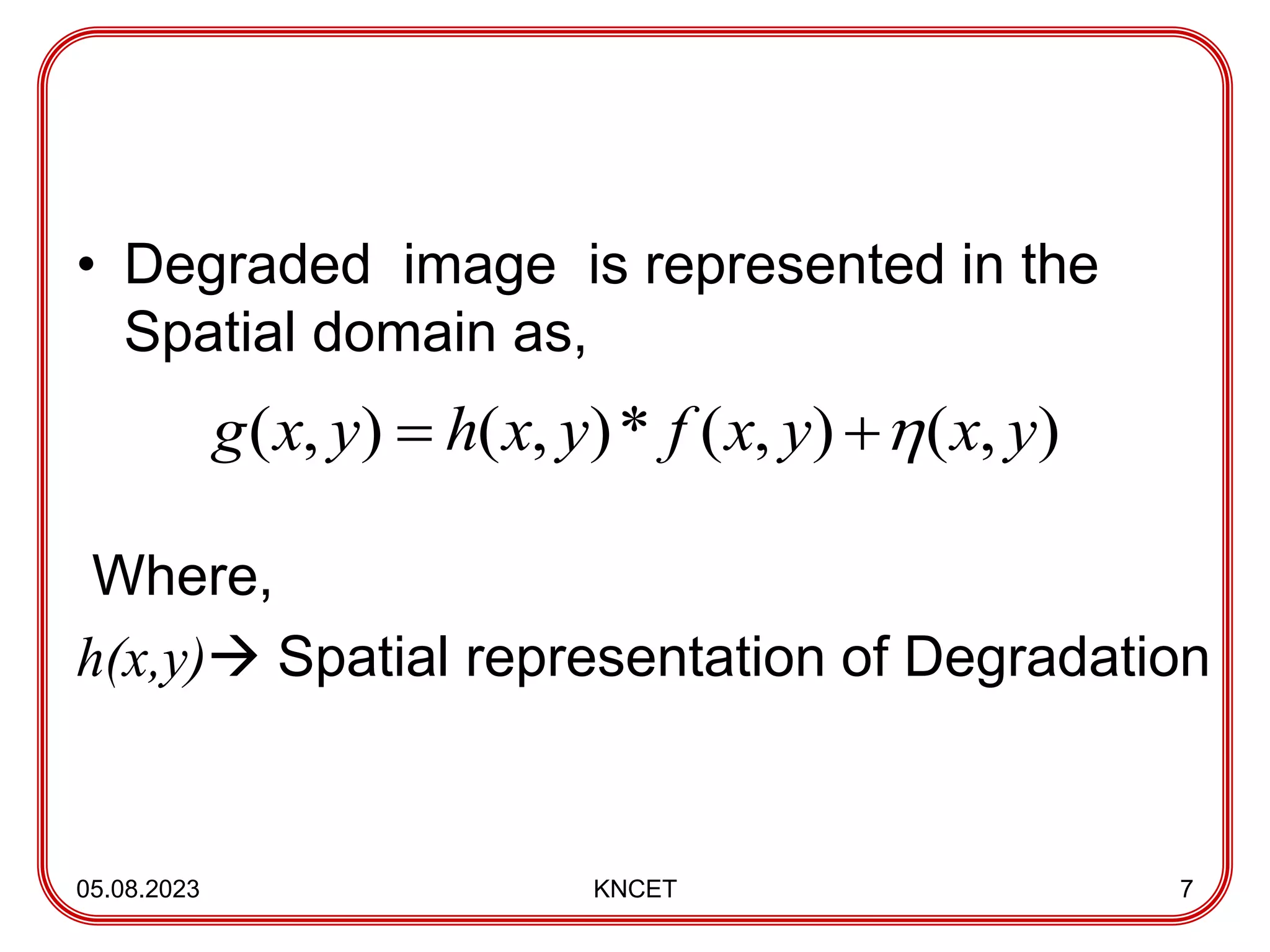
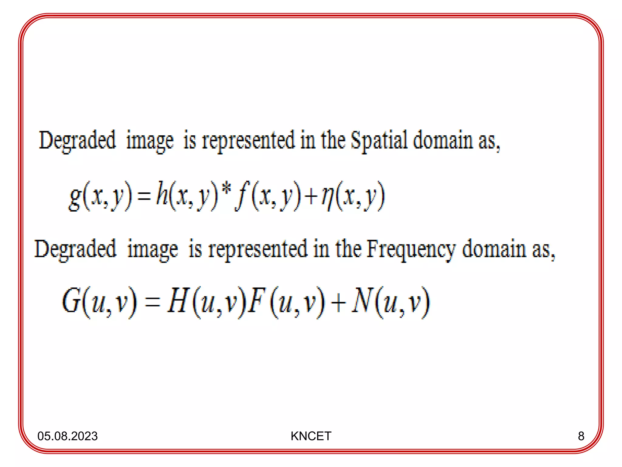
7. • Degraded image is represented in the
Spatial domain as,
Where,
h(x,y) Spatial representation of Degradation
05.08.2023 KNCET 7
)
,
(
)
,
(
*
)
,
(
)
,
( y
x
y
x
f
y
x
h
y
x
g 



8. 05.08.2023 KNCET 8

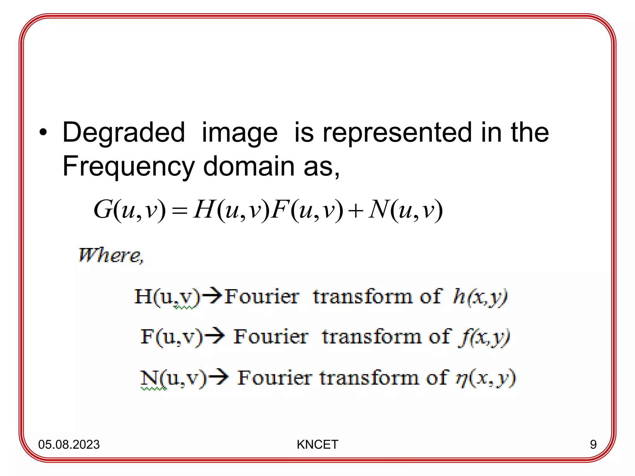
9. • Degraded image is represented in the
Frequency domain as,
05.08.2023 KNCET 9
)
,
(
)
,
(
)
,
(
)
,
( v
u
N
v
u
F
v
u
H
v
u
G 


10. Noise models
• The sources of noise in digital images arise during image
acquisition and transmission
– Imaging sensors can be affected by Environmental
conditions
– Interference can be added to an image during
transmission
• Noise cannot be predicted but can be approximately
described in statistical way using the probability density
function (PDF).
05.08.2023 KNCET 10

11. • Some Noise Probability Density functions
(PDF) are,
1) Gaussian Noise
2) Rayleigh Noise
3) Erlang(Gamma) Noise
4) Exponential Noise
5) Uniform Noise
6) Impulse(Salt and Pepper) Noise
05.08.2023 KNCET 11

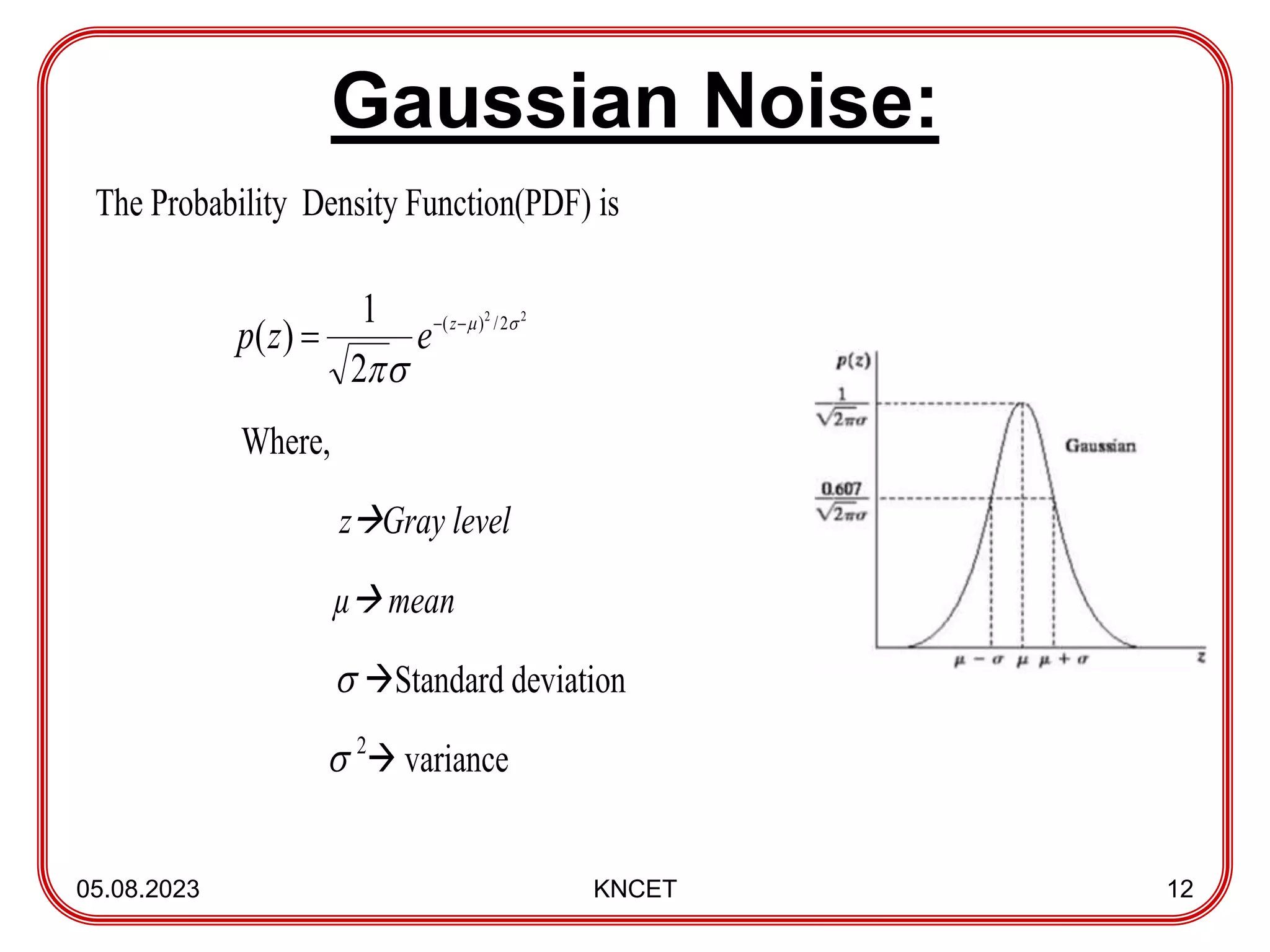
12. Gaussian Noise:
05.08.2023 KNCET 12
The Probability Density Function(PDF) is
Where,
zGray level
µ mean
 Standard deviation
 2
 variance
2
2
2
/
)
(
2
1
)
( 





 z
e
z
p

13. 05.08.2023 KNCET 13
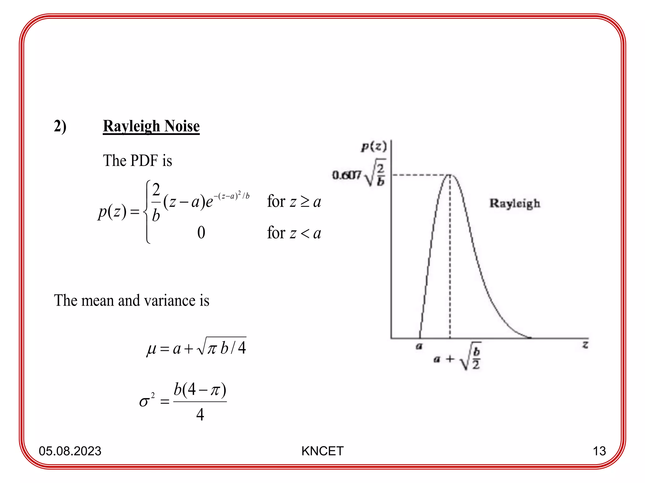
2) Rayleigh Noise
The PDF is
The mean and variance is











a
z
a
z
e
a
z
b
z
p
b
a
z
for
0
for
)
(
2
)
(
/
)
( 2
4
/
b
a 
 

4
)
4
(
2 



b

14. 05.08.2023 KNCET 14
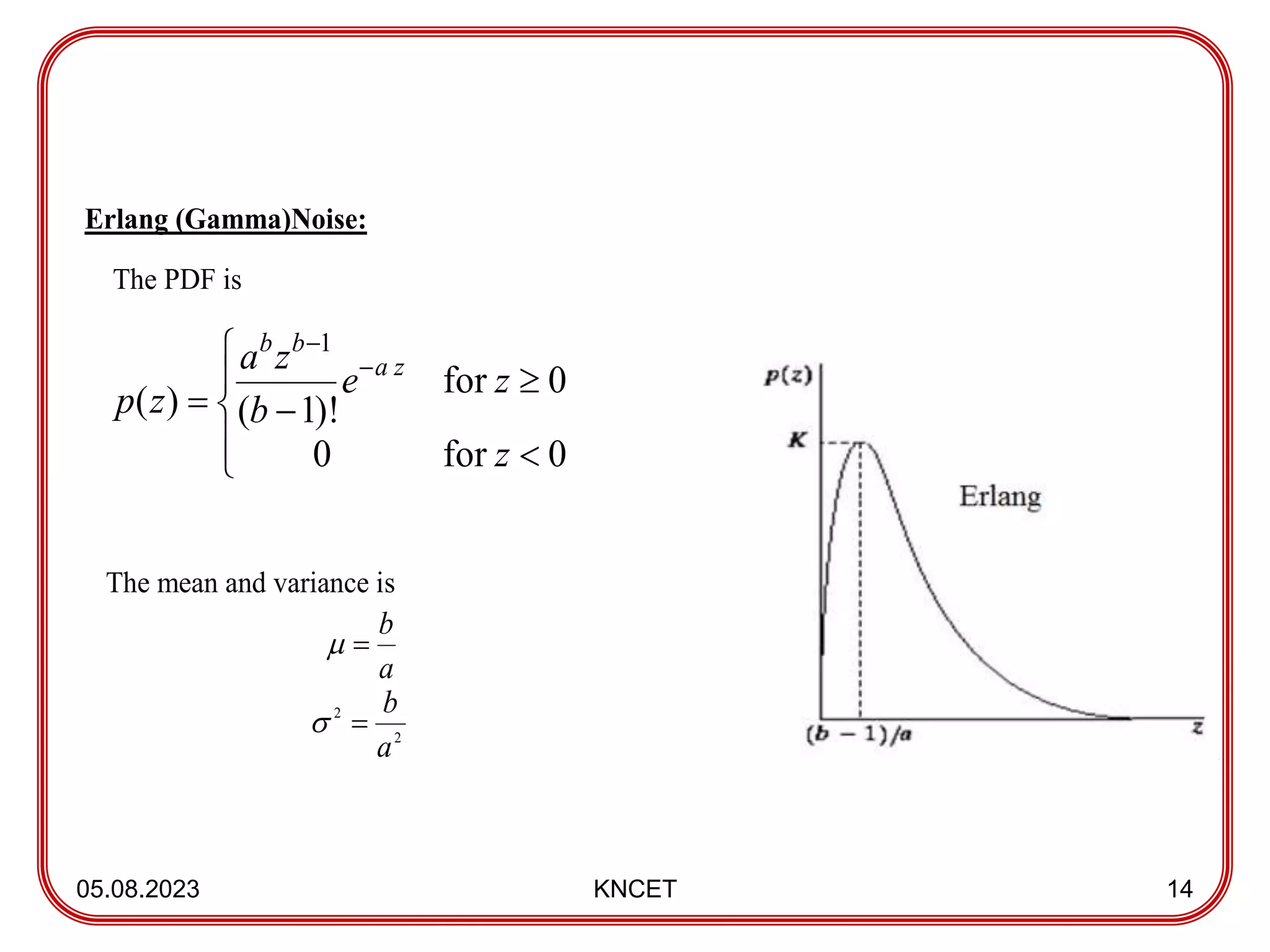
Erlang (Gamma)Noise:
The PDF is
The mean and variance is











0
for
0
0
for
)!
1
(
)
(
1
z
z
e
b
z
a
z
p
z
a
b
b
a
b


2
2
a
b



15. 05.08.2023 KNCET 15
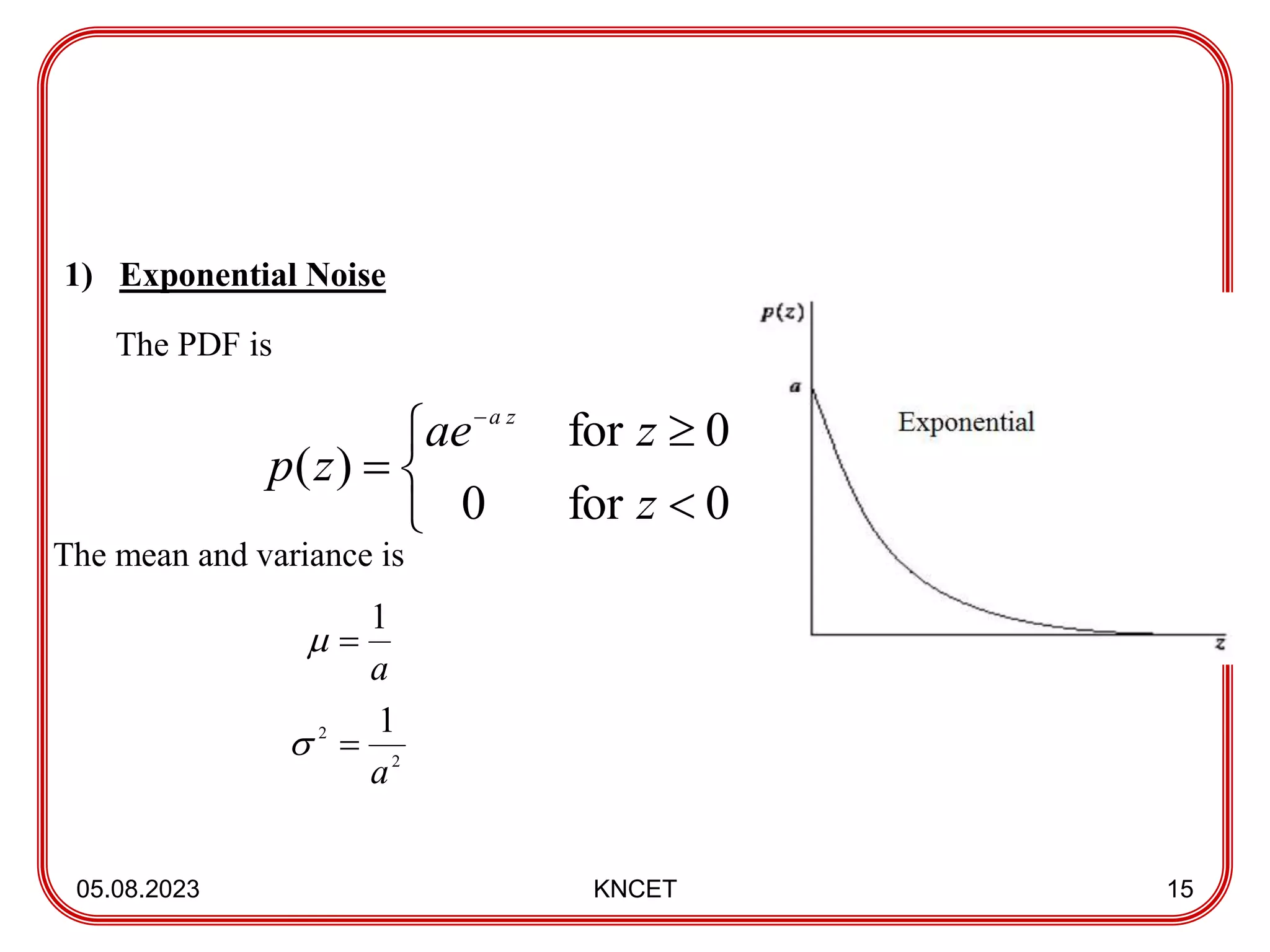
1) Exponential Noise
The PDF is
The mean and variance is







0
for
0
0
for
)
(
z
z
ae
z
p
z
a
a
1


2
2 1
a



16. 05.08.2023 KNCET 16
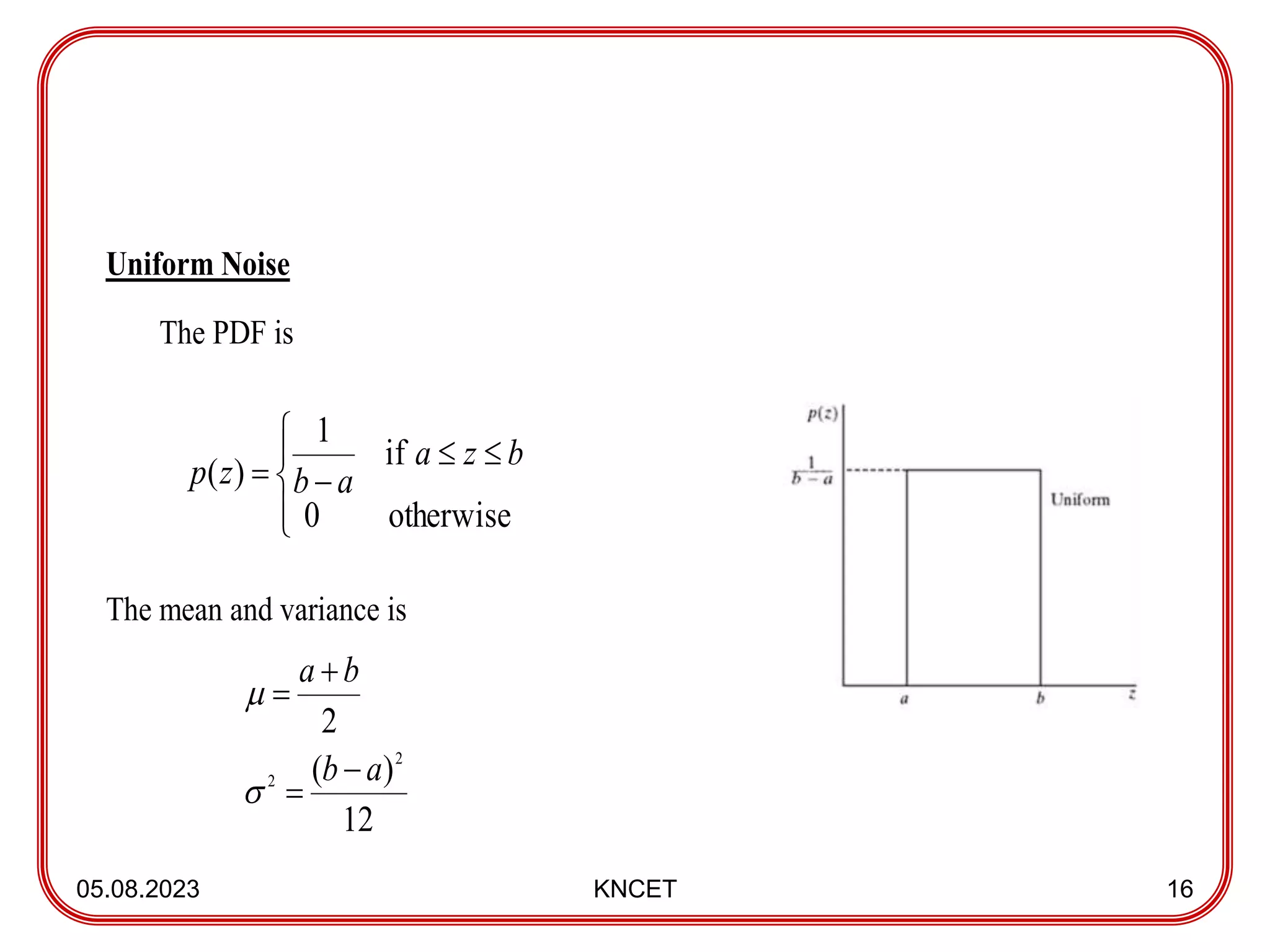
Uniform Noise
The PDF is
The mean and variance is









otherwise
0
if
1
)
(
b
z
a
a
b
z
p
12
)
(
2
2
2 a
b
b
a







17. 05.08.2023 KNCET 17
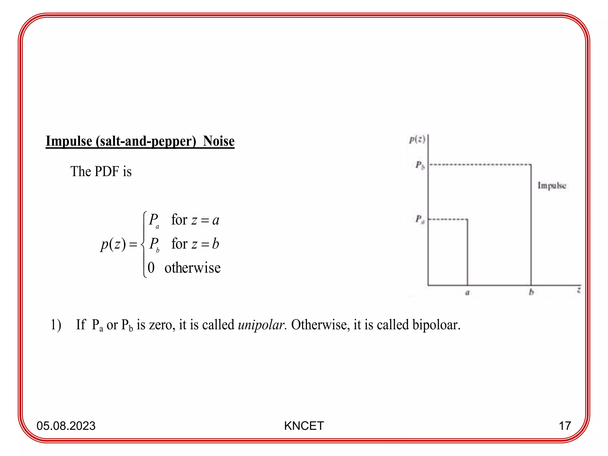
Impulse (salt-and-pepper) Noise
The PDF is
1) If Pa or Pb is zero, it is called unipolar. Otherwise, it is called bipoloar.








otherwise
0
for
for
)
( b
z
P
a
z
P
z
p b
a

18. Mean filters
It replaces the value of every pixel in an image by
the average (or) mean of the gray levels in the
neighborhood of that pixel.
It is also called as Averaging filter.
Mean filters are the spatial filters which are used
for noise reduction.
05.08.2023 KNCET 18

19. Types:
1) Arithmetic Mean filter
2) Geometric Mean filter
3) Harmonic Mean filter
4) Contraharmonic Mean filter
05.08.2023 KNCET 19

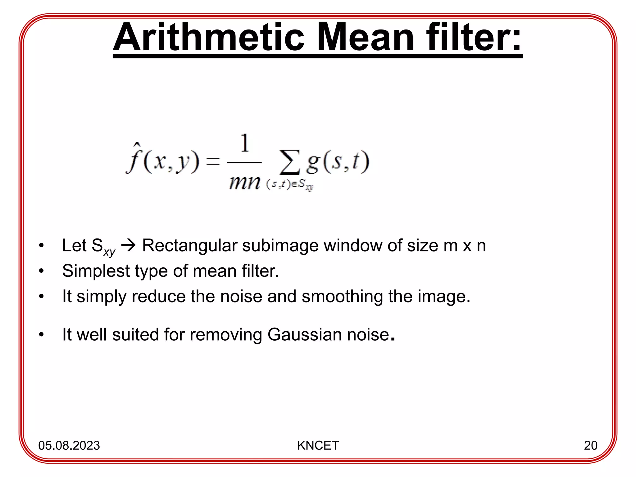
20. Arithmetic Mean filter:
• Let Sxy  Rectangular subimage window of size m x n
• Simplest type of mean filter.
• It simply reduce the noise and smoothing the image.
• It well suited for removing Gaussian noise.
05.08.2023 KNCET 20

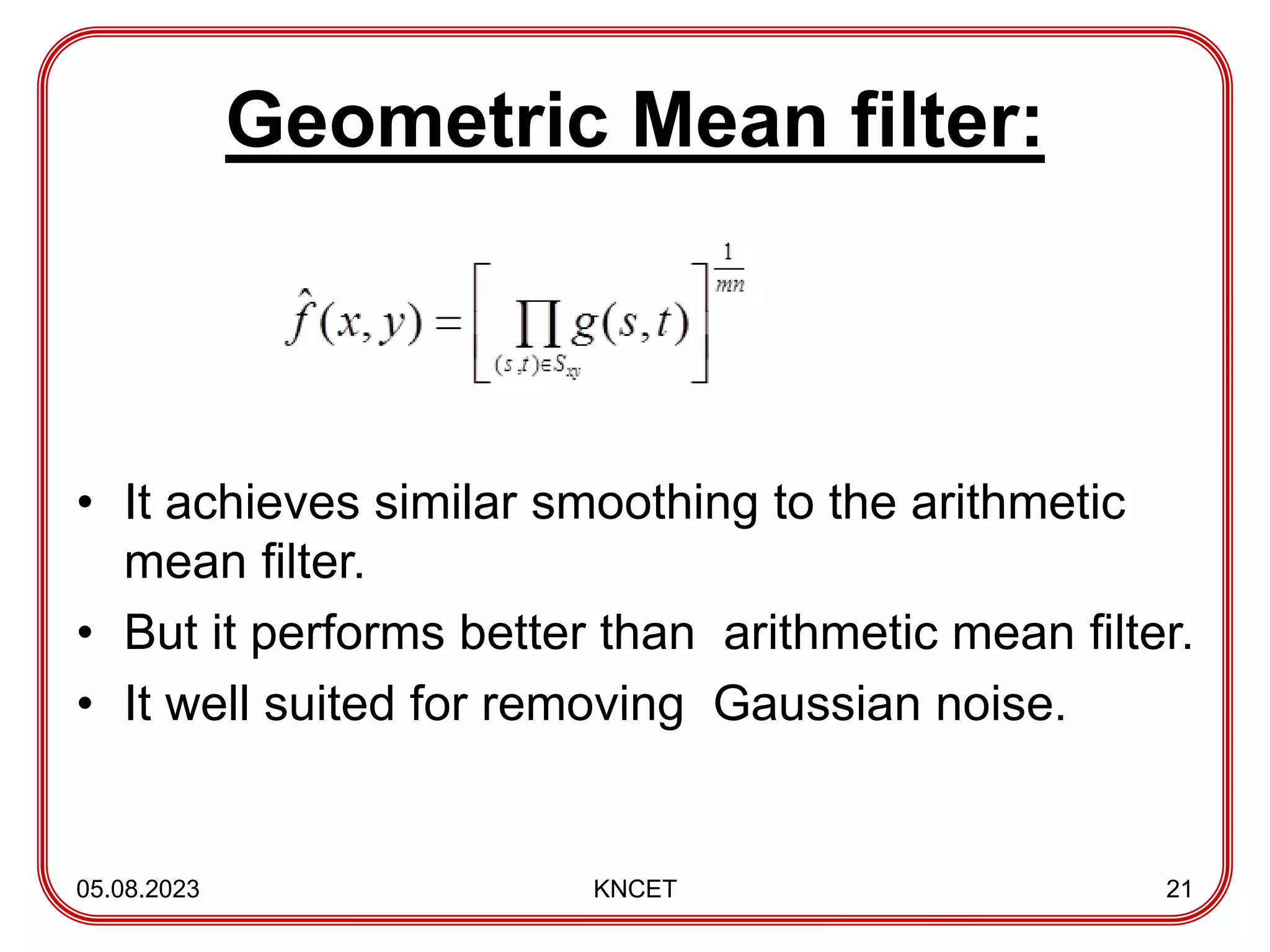
21. Geometric Mean filter:
• It achieves similar smoothing to the arithmetic
mean filter.
• But it performs better than arithmetic mean filter.
• It well suited for removing Gaussian noise.
05.08.2023 KNCET 21

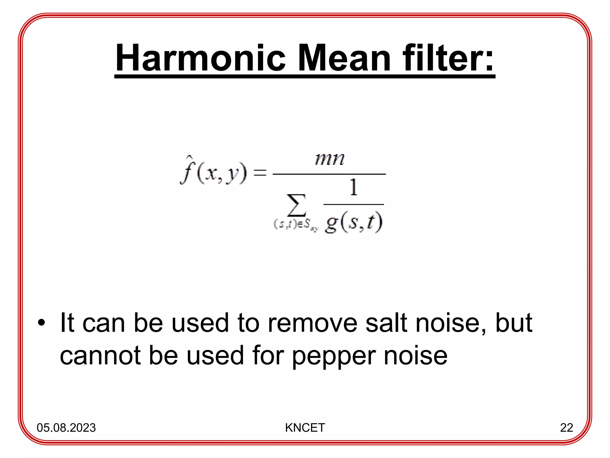
22. Harmonic Mean filter:
• It can be used to remove salt noise, but
cannot be used for pepper noise
05.08.2023 KNCET 22

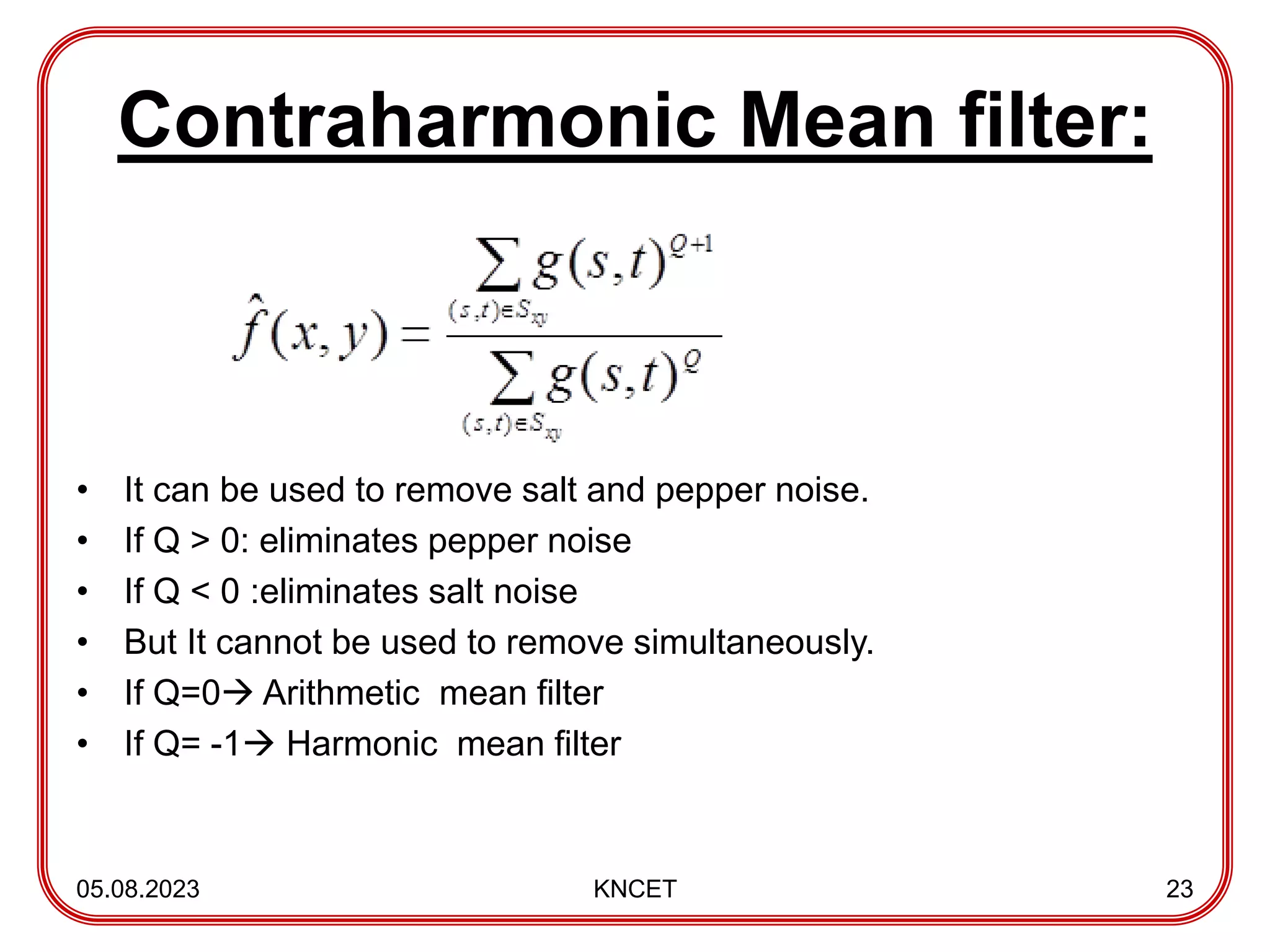
23. Contraharmonic Mean filter:
• It can be used to remove salt and pepper noise.
• If Q > 0: eliminates pepper noise
• If Q < 0 :eliminates salt noise
• But It cannot be used to remove simultaneously.
• If Q=0 Arithmetic mean filter
• If Q= -1 Harmonic mean filter
05.08.2023 KNCET 23

24. Order Statistics Filters
• It is based on ordering(ranking) of the values of
the pixels. It replacing the value of the center
pixel with the value determined by the ranking
result.
• Order-statistics filters are nonlinear spatial
filters.
05.08.2023 KNCET 24

25. Concept:
• First, the values of the pixels covered by the filter mask
are ordered. i.e., ranked ascending order (from
minimum to maximum).
• Then, the value of the center pixel is replaced by the
value of the ranking result.
05.08.2023 KNCET 25

26. Types:
– Median filter
– Max and Min filter
– Midpoint filter
– Alpha trimmed mean filter
05.08.2023 KNCET 26

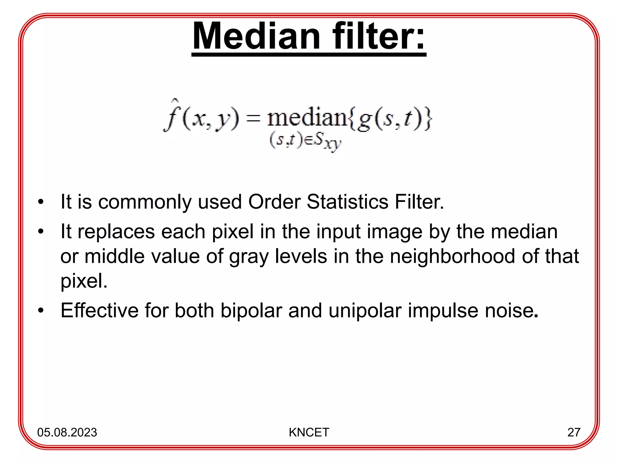
27. Median filter:
• It is commonly used Order Statistics Filter.
• It replaces each pixel in the input image by the median
or middle value of gray levels in the neighborhood of that
pixel.
• Effective for both bipolar and unipolar impulse noise.
05.08.2023 KNCET 27

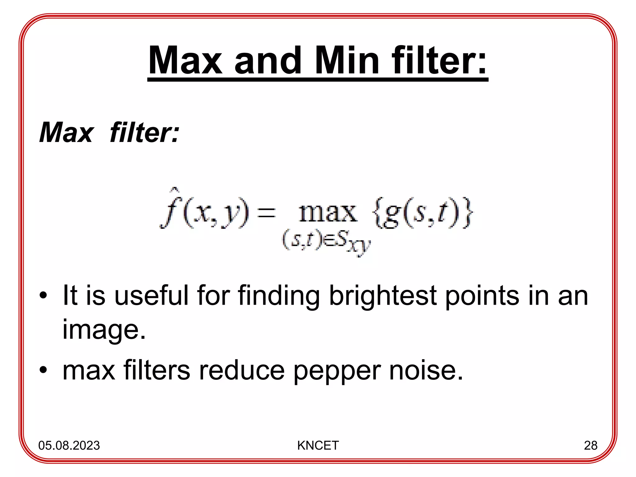
28. Max and Min filter:
Max filter:
• It is useful for finding brightest points in an
image.
• max filters reduce pepper noise.
05.08.2023 KNCET 28

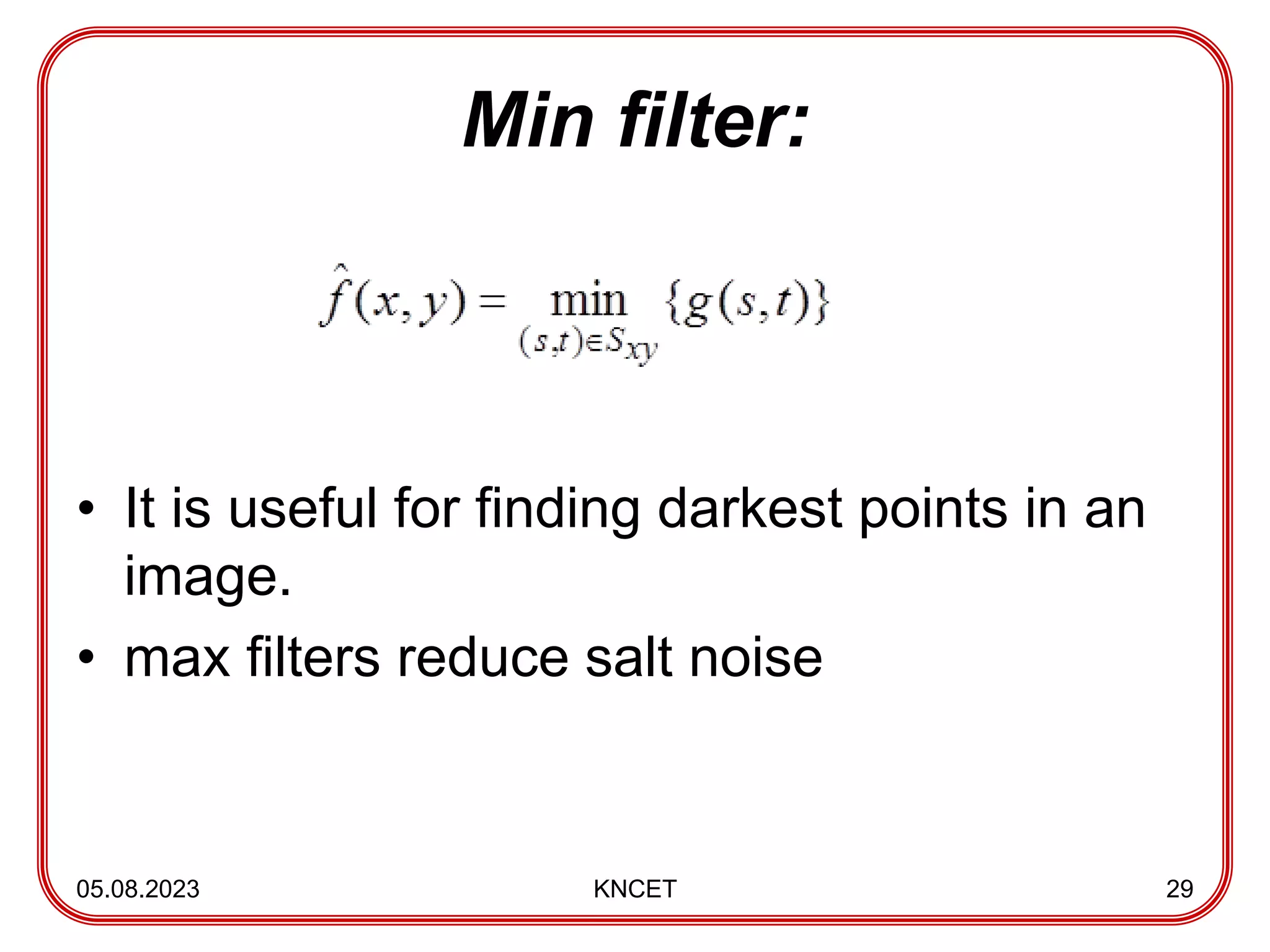
29. Min filter:
• It is useful for finding darkest points in an
image.
• max filters reduce salt noise
05.08.2023 KNCET 29

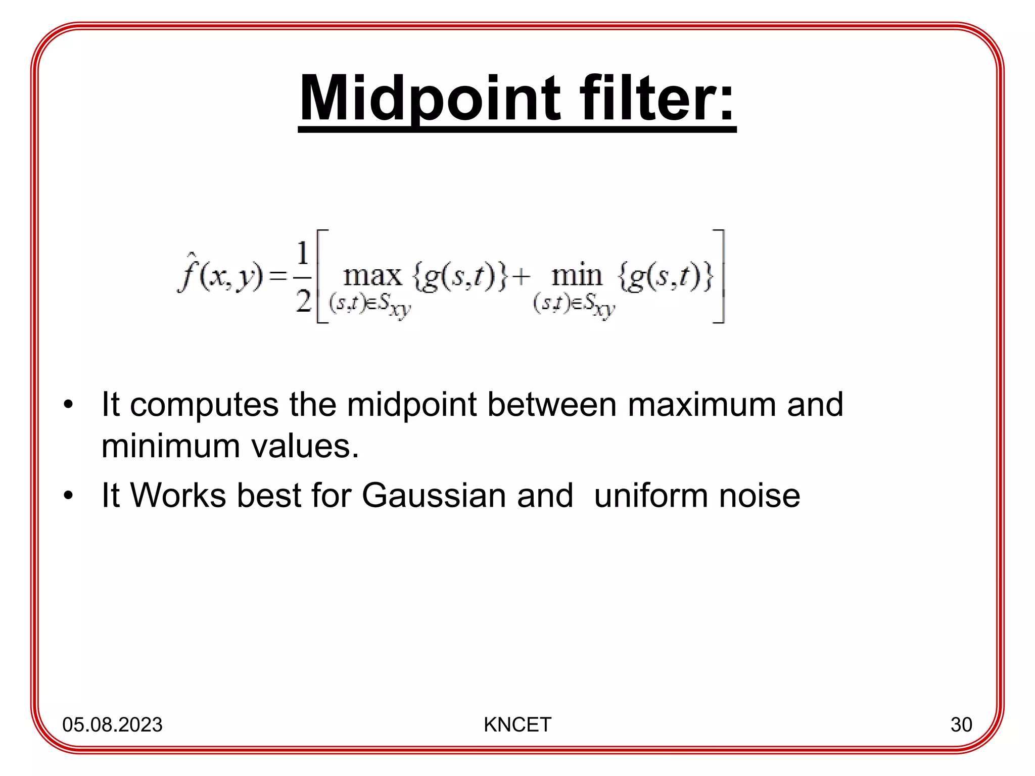
30. Midpoint filter:
• It computes the midpoint between maximum and
minimum values.
• It Works best for Gaussian and uniform noise
05.08.2023 KNCET 30

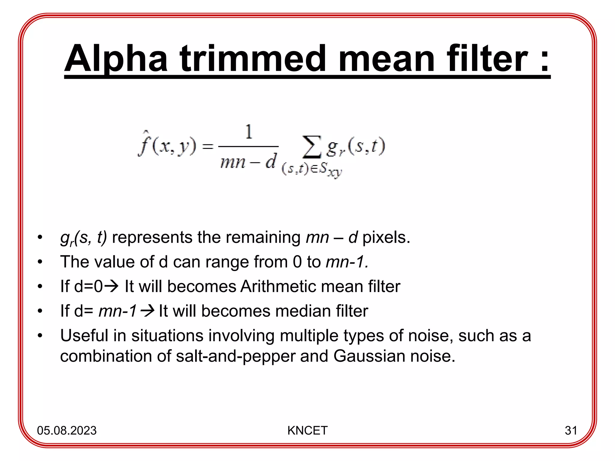
31. Alpha trimmed mean filter :
• gr(s, t) represents the remaining mn – d pixels.
• The value of d can range from 0 to mn-1.
• If d=0 It will becomes Arithmetic mean filter
• If d= mn-1 It will becomes median filter
• Useful in situations involving multiple types of noise, such as a
combination of salt-and-pepper and Gaussian noise.
05.08.2023 KNCET 31

32. 05.08.2023 KNCET 32
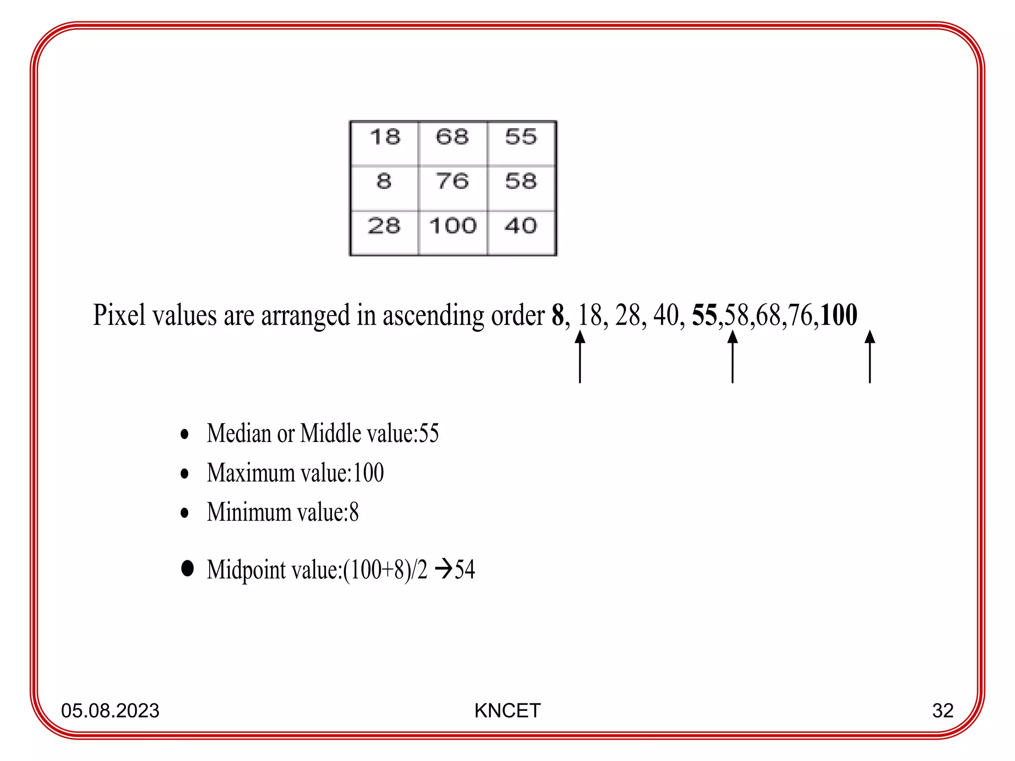
Pixel values are arranged in ascending order 8, 18, 28, 40, 55,58,68,76,100
 Median or Middle value:55
 Maximum value:100
 Minimum value:8
 Midpoint value:(100+8)/2 54

33. Adaptive Filters
• The behaviour of adaptive filters changes
depending on the characteristics of the
image inside the filter region.
Types:
1)Adaptive local noise reduction filter
2)Adaptive Median Filter
05.08.2023 KNCET 33

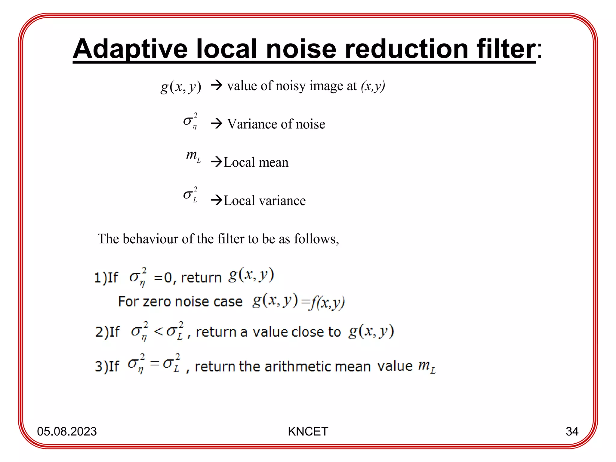
34. Adaptive local noise reduction filter:
05.08.2023 KNCET 34
 value of noisy image at (x,y)
 Variance of noise
Local mean
Local variance
The behaviour of the filter to be as follows,
2


2
L

)
,
( y
x
g
L
m

35. • Adaptive filter expression may be written as,
05.08.2023 KNCET 35

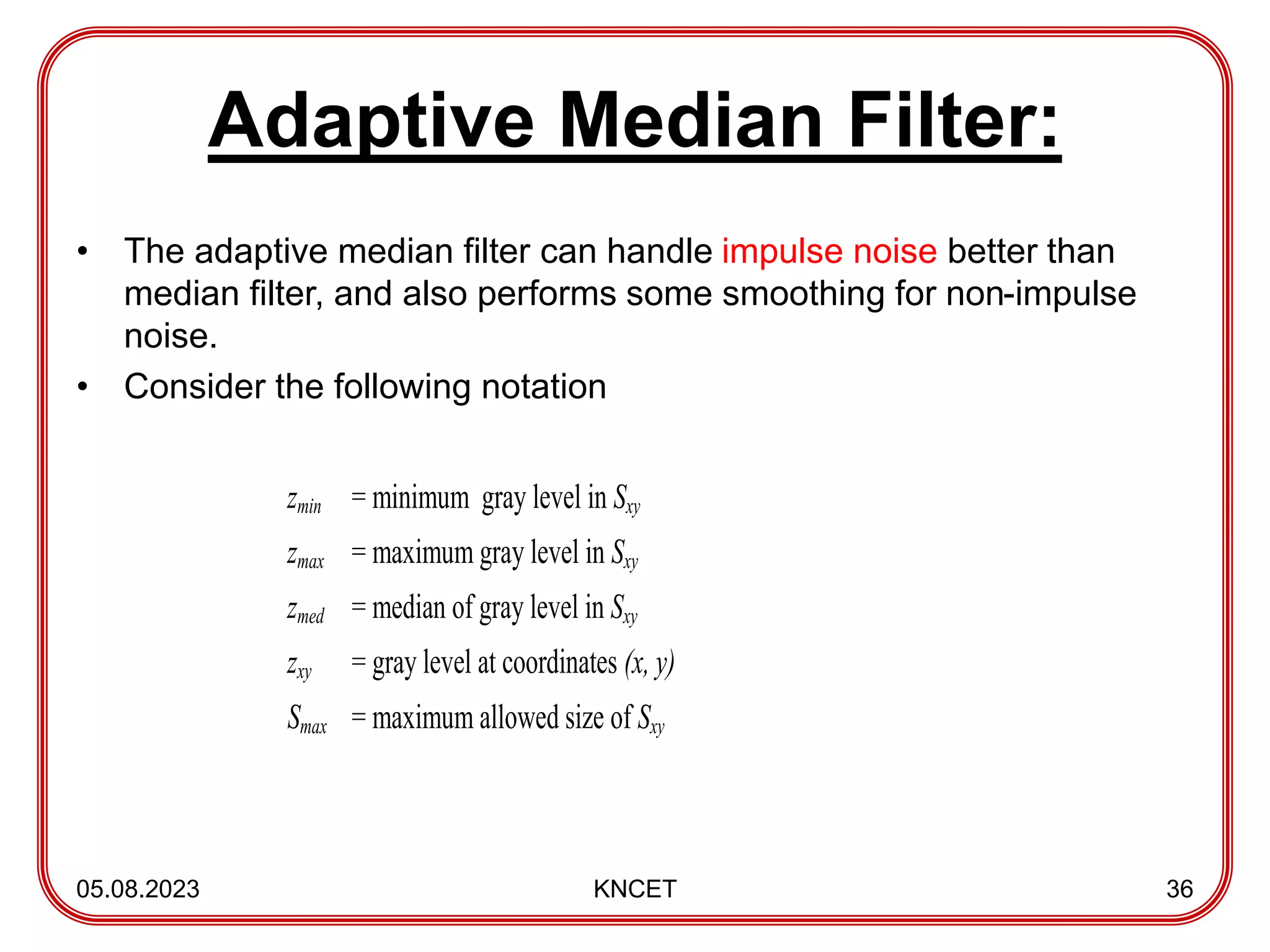
36. Adaptive Median Filter:
• The adaptive median filter can handle impulse noise better than
median filter, and also performs some smoothing for non-impulse
noise.
• Consider the following notation
05.08.2023 KNCET 36
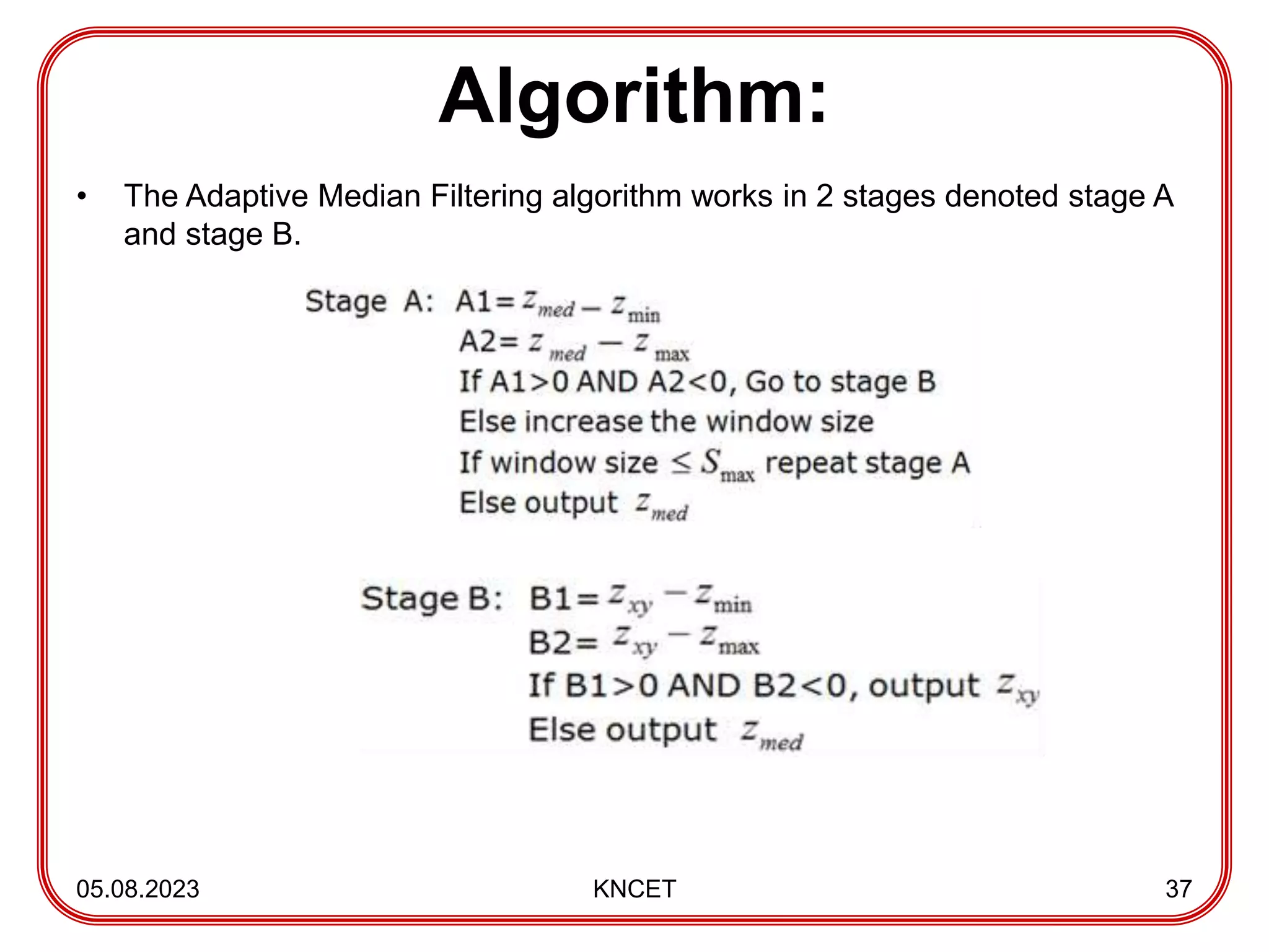
zmin = minimum gray level in Sxy
zmax = maximum gray level in Sxy
zmed = median of gray level in Sxy
zxy = gray level at coordinates (x, y)
Smax = maximum allowed size of Sxy

37. Algorithm:
• The Adaptive Median Filtering algorithm works in 2 stages denoted stage A
and stage B.
05.08.2023 KNCET 37

38. Purposes of the algorithm:
• Remove salt-and-pepper (impulse) noise
• Provide smoothing
• Reduce distortion
Periodic Noise Reduction by Frequency Domain Filtering
• Bandreject filter
• Band Pass Filter
• Notch Filter
05.08.2023 KNCET 38

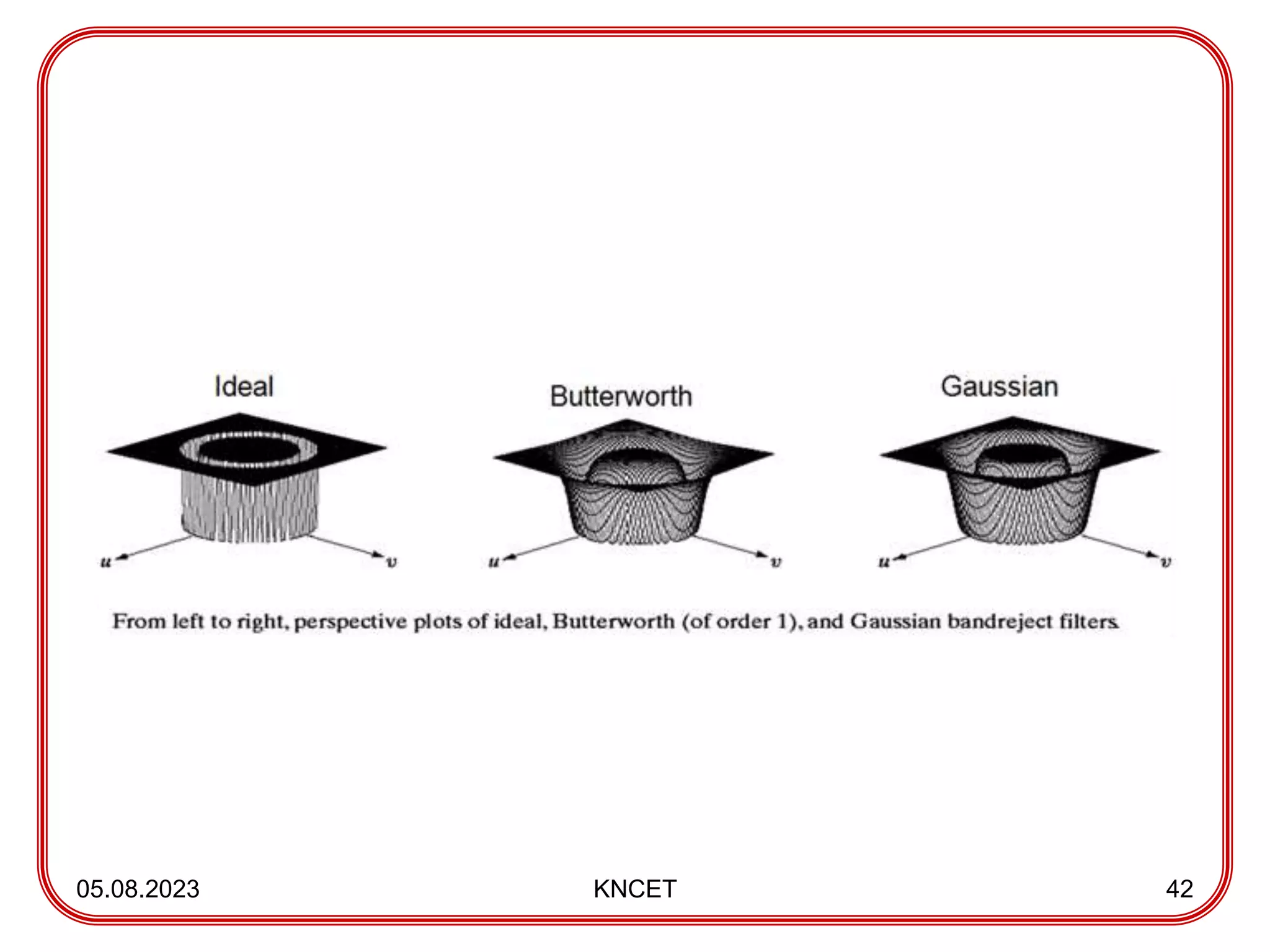
39. Band Reject filter
• It removing periodic noise form an image that involves
removing a particular range of frequencies from that
image.
Types:
• Ideal Band Reject Filter
• Butterworth Band Reject Filter
• Gaussian Band Reject Filter
05.08.2023 KNCET 39

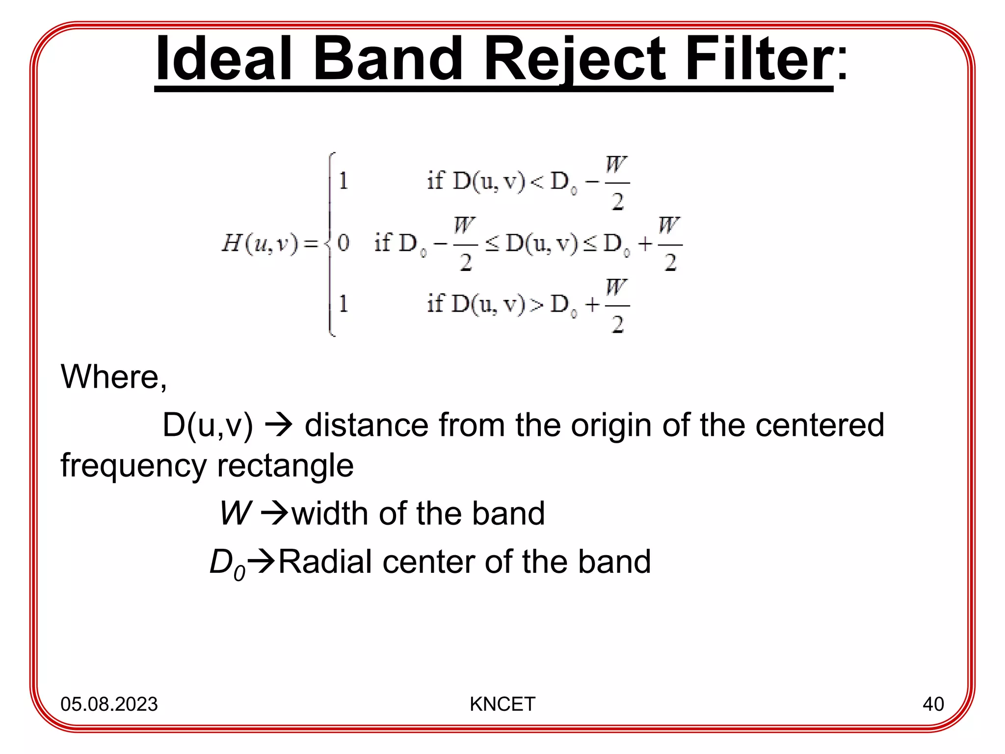
40. Ideal Band Reject Filter:
Where,
D(u,v)  distance from the origin of the centered
frequency rectangle
W width of the band
D0Radial center of the band
05.08.2023 KNCET 40

41. Butterworth Band Reject Filter:
05.08.2023 KNCET 41
 Gaussian Band Reject Filter:
2
2
0
2
)
,
(
)
,
(
2
1
1
)
,
( 






 



W
v
u
D
D
v
u
D
e
v
u
H

42. 05.08.2023 KNCET 42

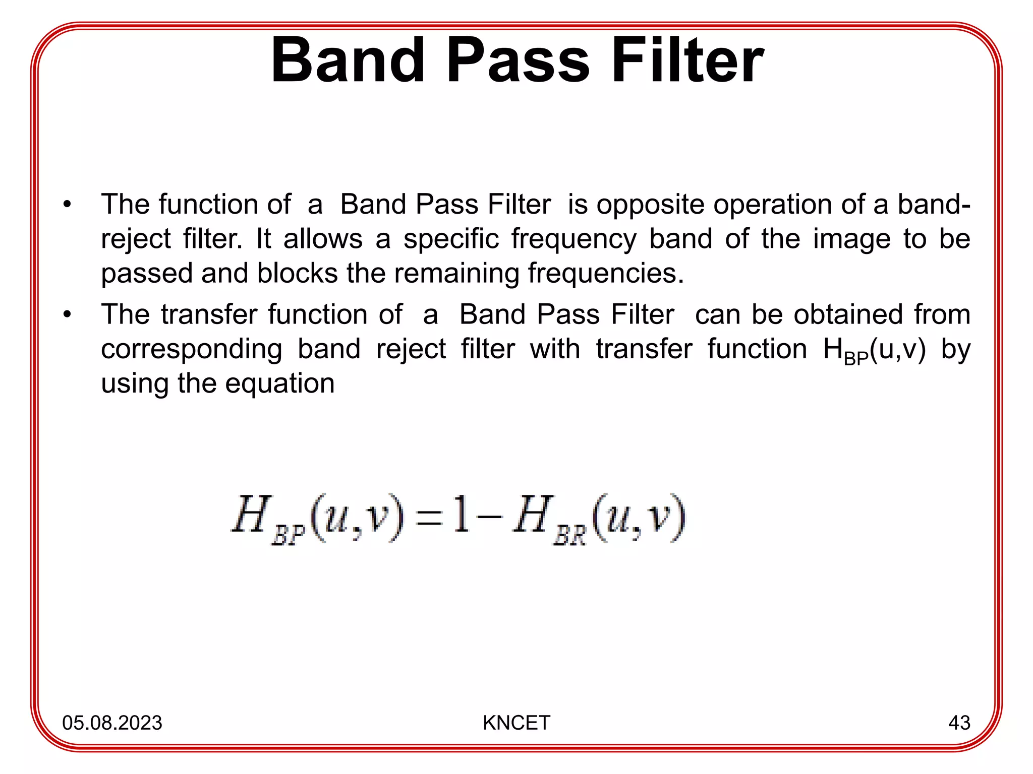
43. Band Pass Filter
• The function of a Band Pass Filter is opposite operation of a band-
reject filter. It allows a specific frequency band of the image to be
passed and blocks the remaining frequencies.
• The transfer function of a Band Pass Filter can be obtained from
corresponding band reject filter with transfer function HBP(u,v) by
using the equation
05.08.2023 KNCET 43

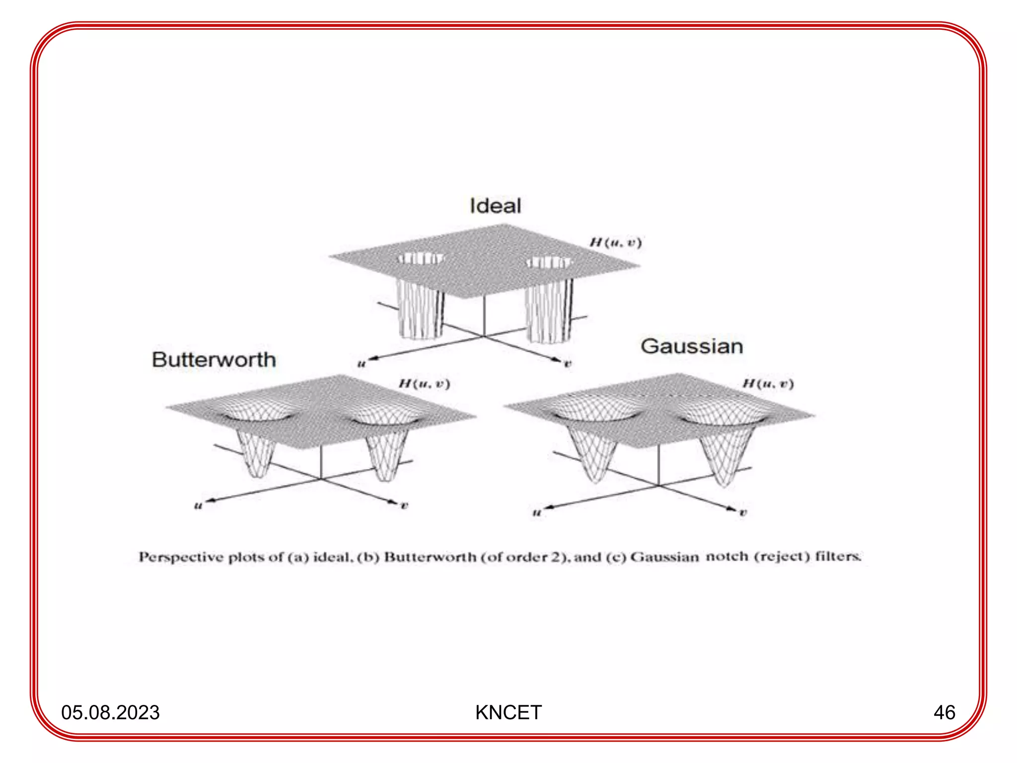
44. Notch Filters
It rejects frequencies in predefined neighborhoods about a center frequency.
These filters are symmetric about origin in the Fourier transform.
Types:
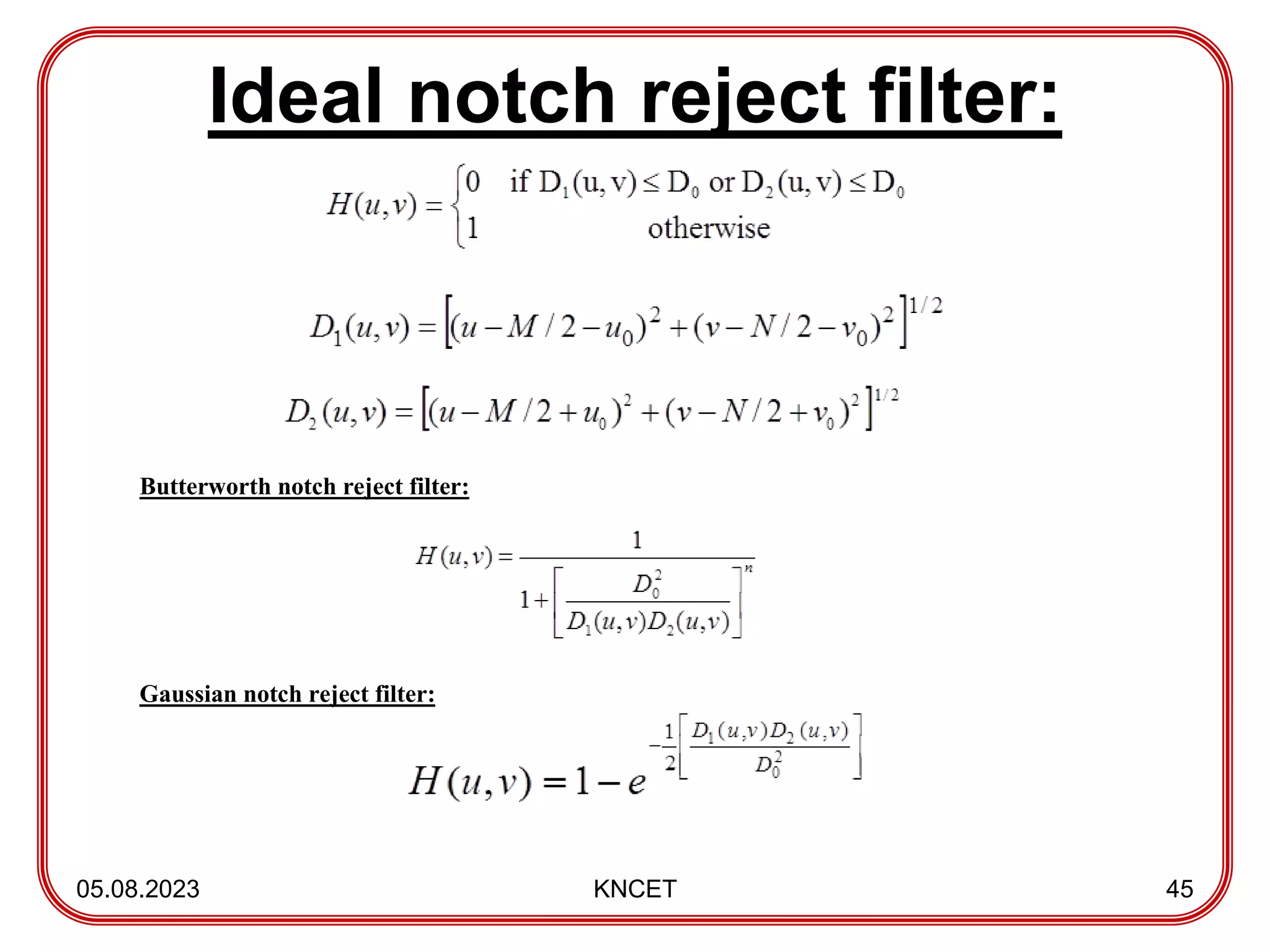
Ideal notch reject filter
Butterworth notch reject filter
Gaussian notch reject filter
05.08.2023 KNCET 44

45. Ideal notch reject filter:
05.08.2023 KNCET 45
Butterworth notch reject filter:
Gaussian notch reject filter:

46. 05.08.2023 KNCET 46

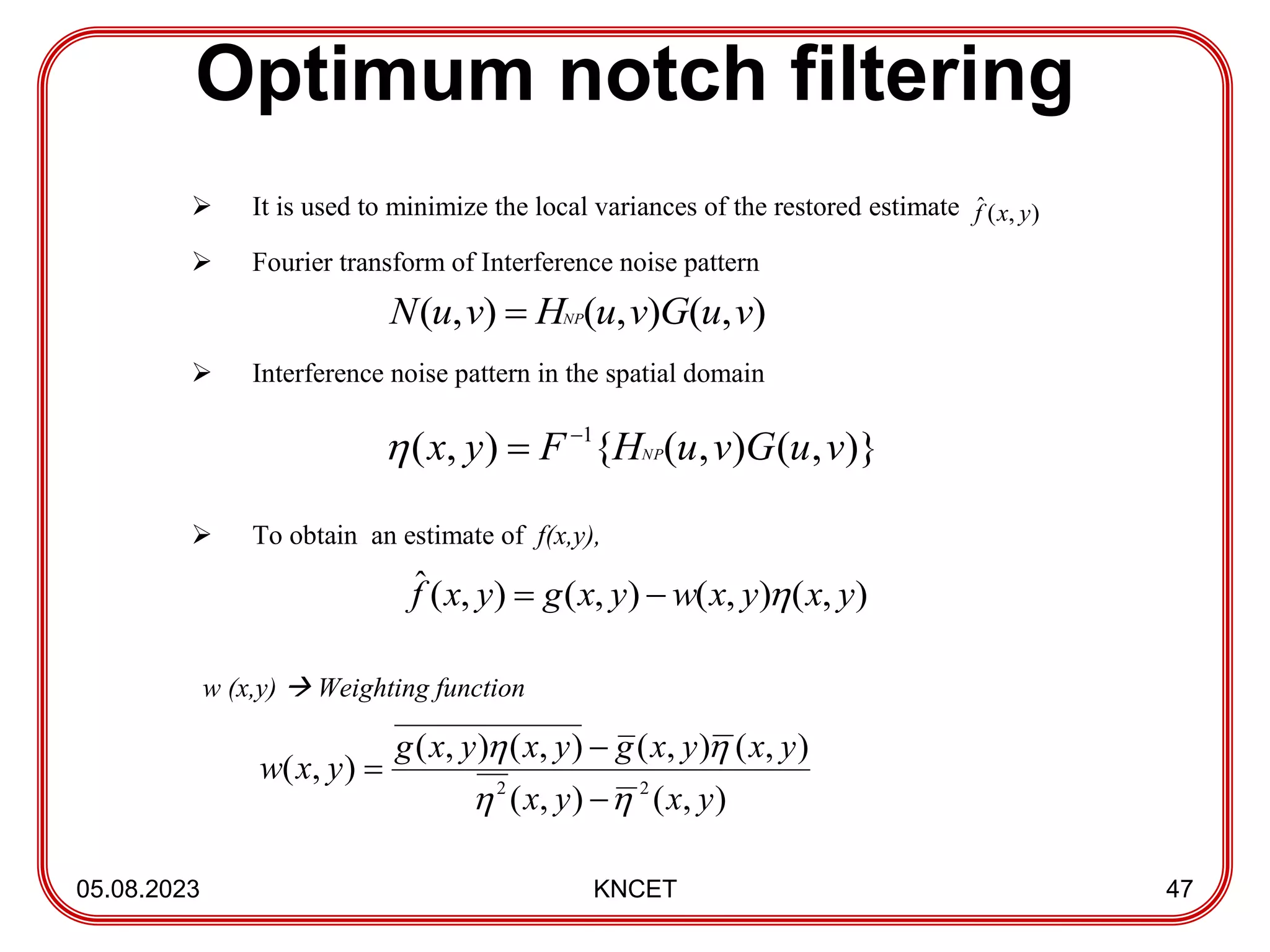
47. Optimum notch filtering
05.08.2023 KNCET 47
 It is used to minimize the local variances of the restored estimate
 Fourier transform of Interference noise pattern
 Interference noise pattern in the spatial domain
 To obtain an estimate of f(x,y),
w (x,y)  Weighting function
)
,
(
ˆ y
x
f
)
,
(
)
,
(
)
,
( v
u
G
v
u
H
v
u
N NP

)}
,
(
)
,
(
{
)
,
( 1
v
u
G
v
u
H
F
y
x NP



)
,
(
)
,
(
)
,
(
)
,
(
ˆ y
x
y
x
w
y
x
g
y
x
f 


)
,
(
)
,
(
)
,
(
)
,
(
)
,
(
)
,
(
)
,
( 2
2
y
x
y
x
y
x
y
x
g
y
x
y
x
g
y
x
w








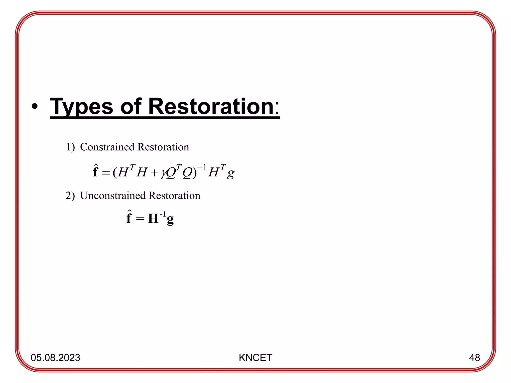
48. • Types of Restoration:
05.08.2023 KNCET 48
1) Constrained Restoration
g
H
Q
Q
H
H T
T
T 1
)
(
ˆ 

 
f
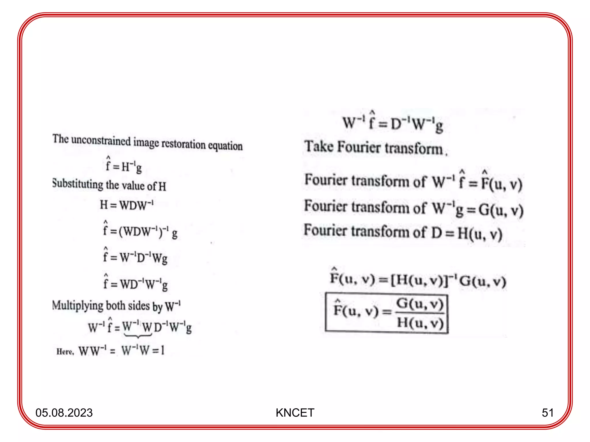
2) Unconstrained Restoration
ˆ -1
f = H g

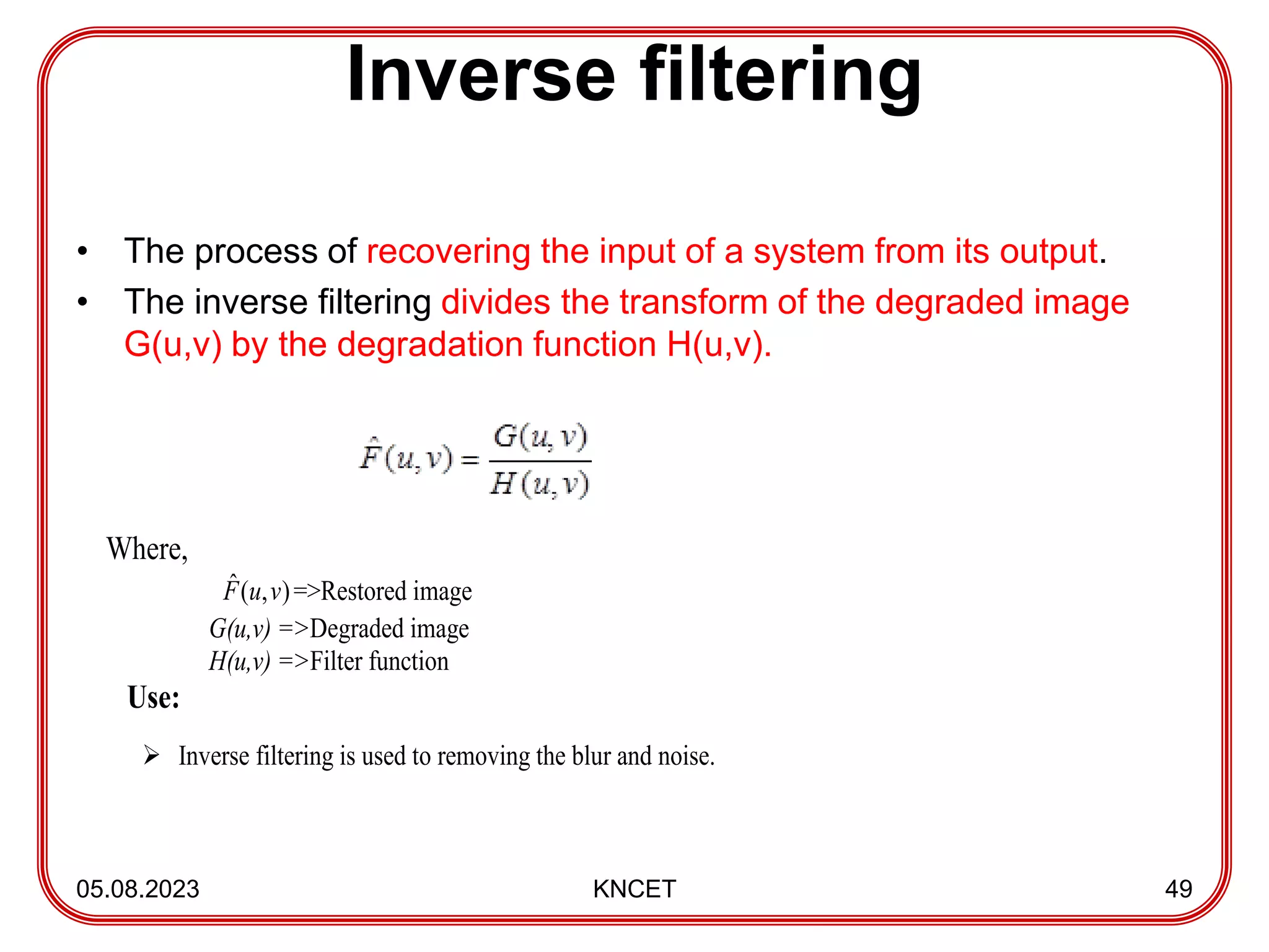
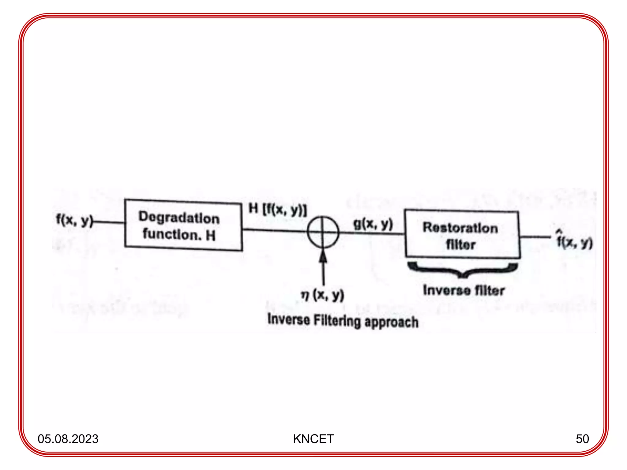
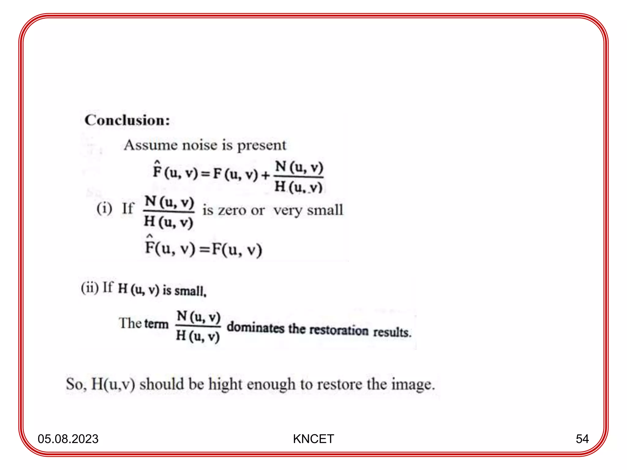
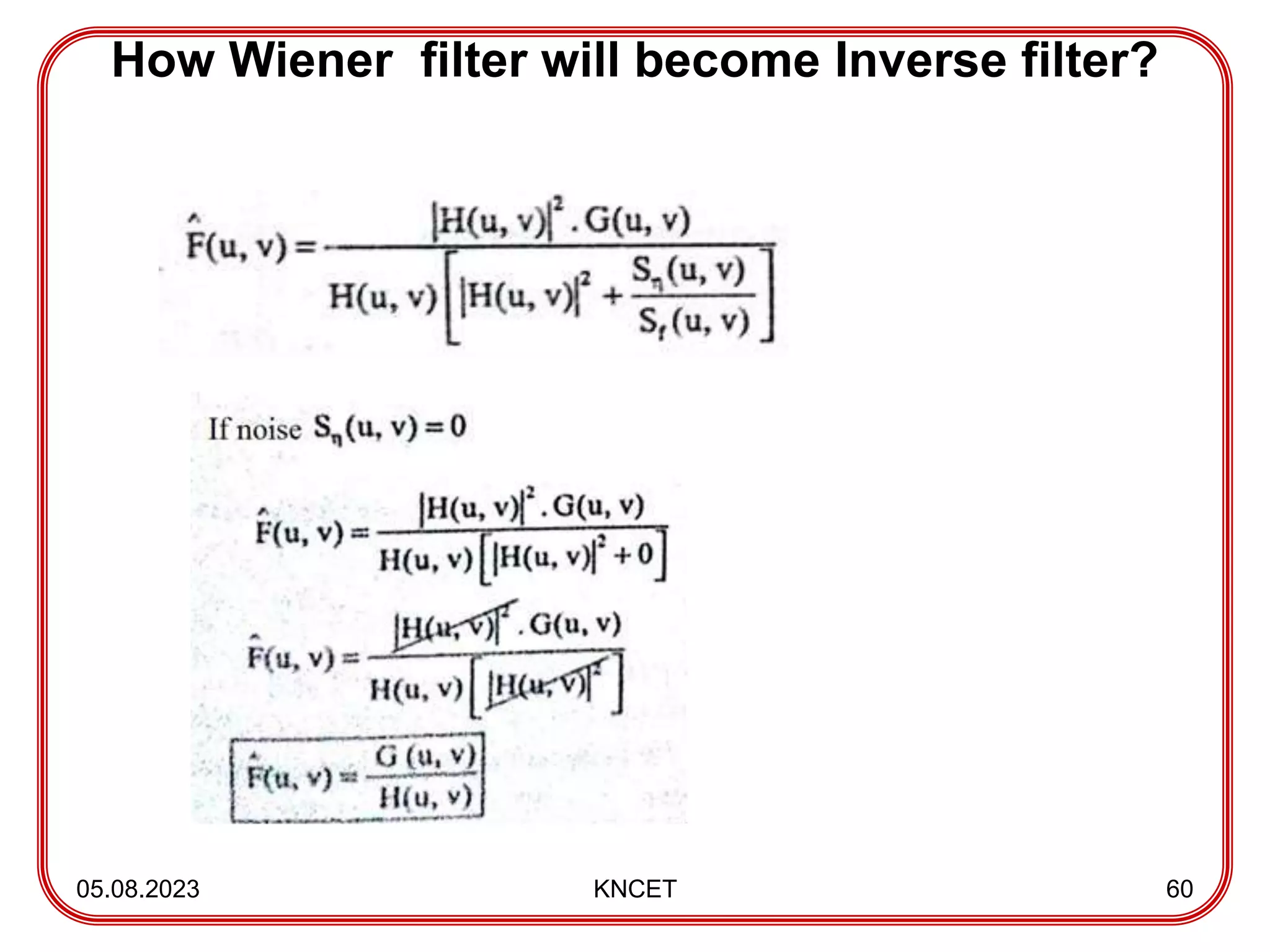
49. Inverse filtering
• The process of recovering the input of a system from its output.
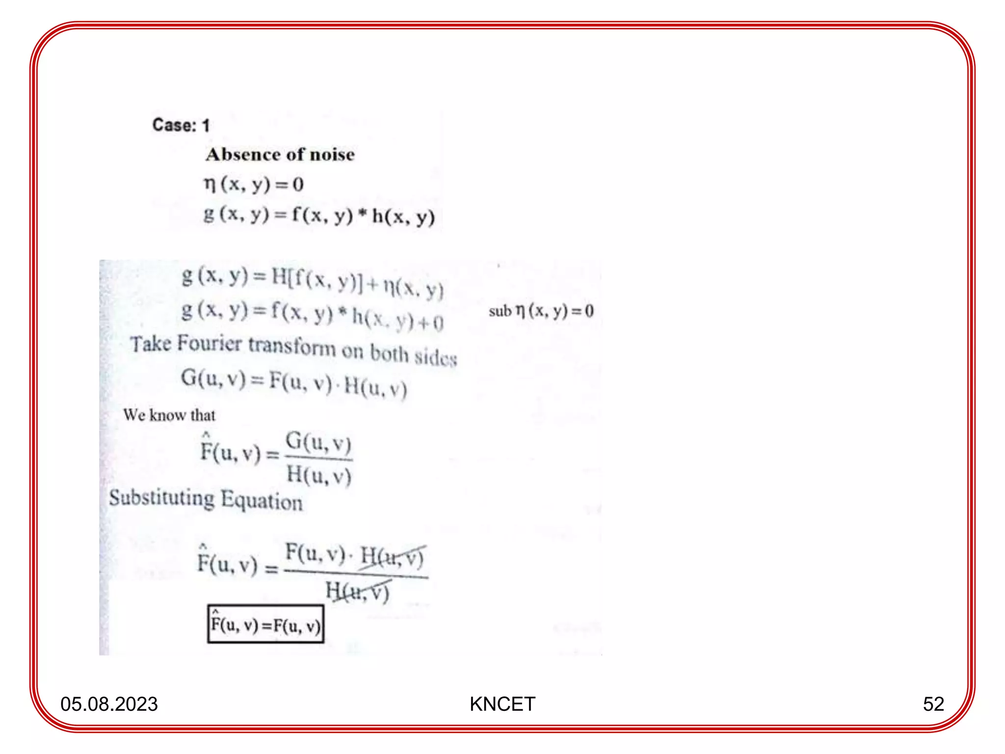
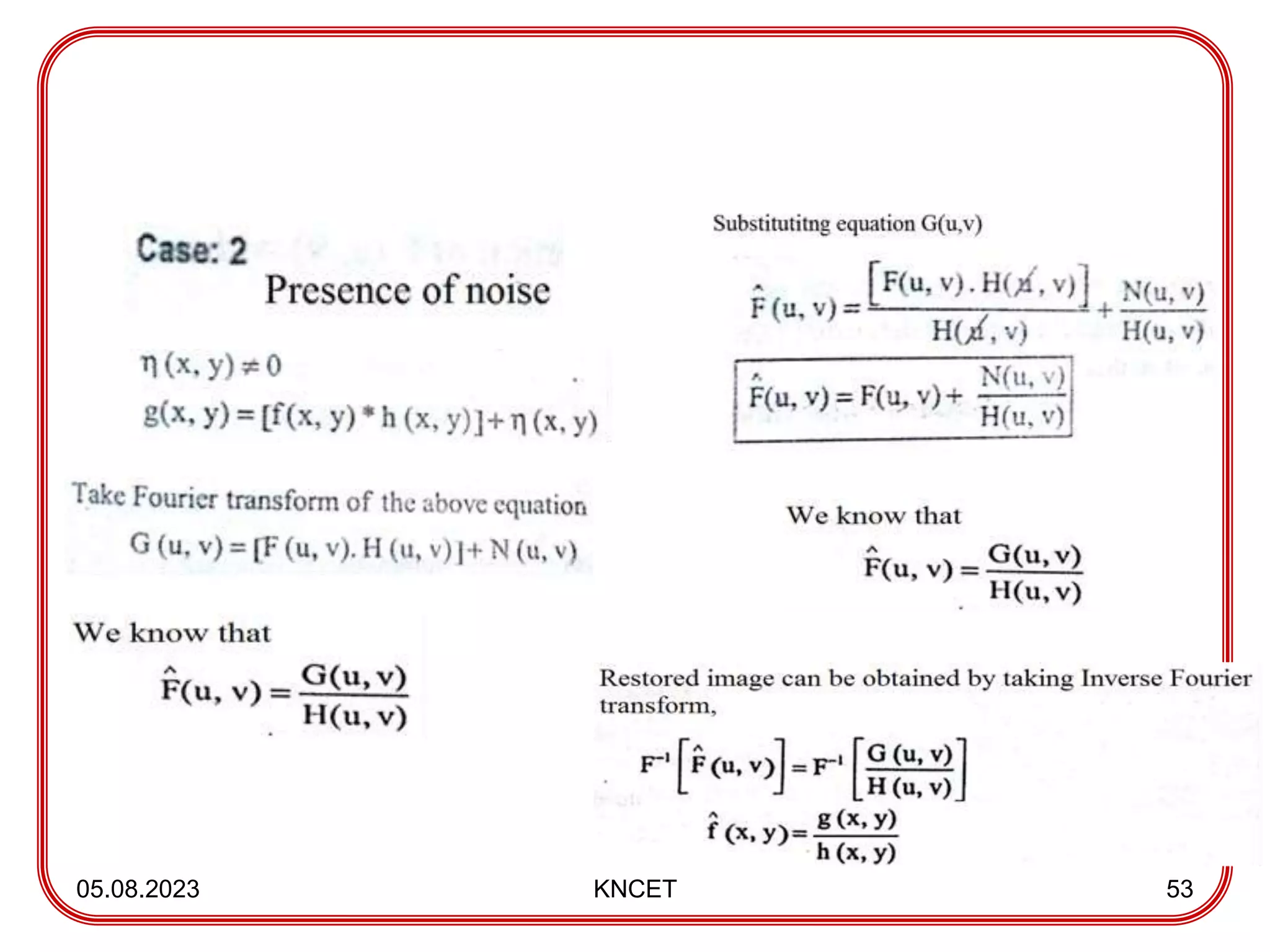
• The inverse filtering divides the transform of the degraded image
G(u,v) by the degradation function H(u,v).
05.08.2023 KNCET 49
Where,
)
,
(
ˆ v
u
F =>Restored image
G(u,v) =>Degraded image
H(u,v) =>Filter function
Use:
 Inverse filtering is used to removing the blur and noise.

50. 05.08.2023 KNCET 50

51. 05.08.2023 KNCET 51

52. 05.08.2023 KNCET 52

53. 05.08.2023 KNCET 53

54. 05.08.2023 KNCET 54

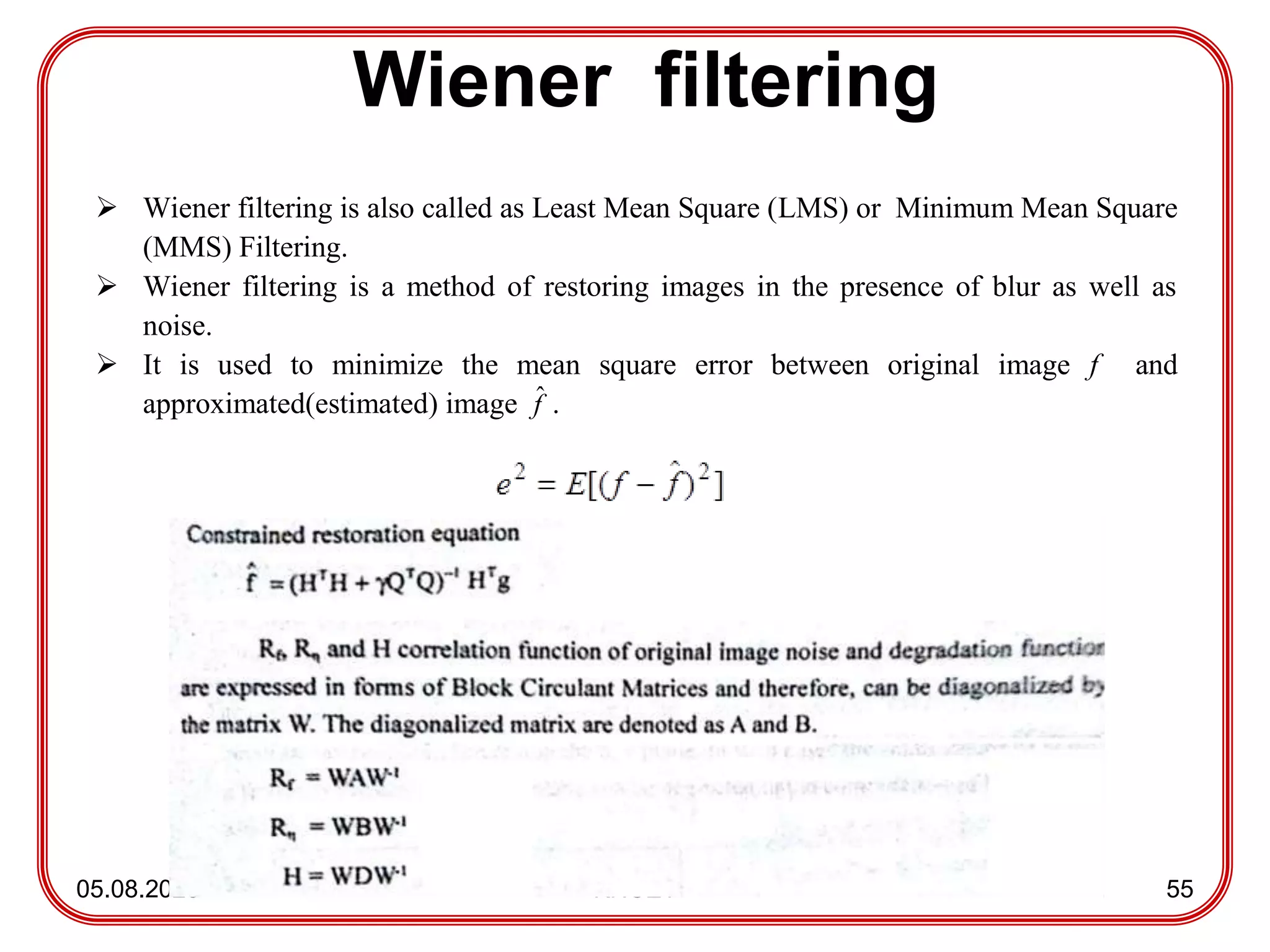
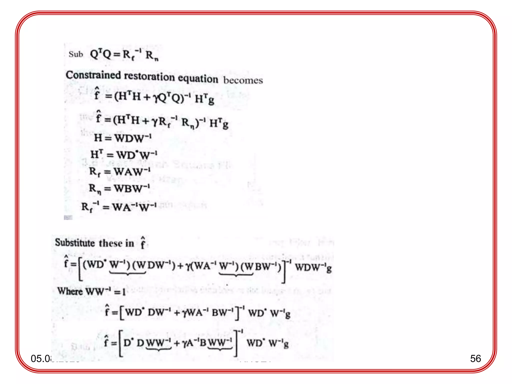
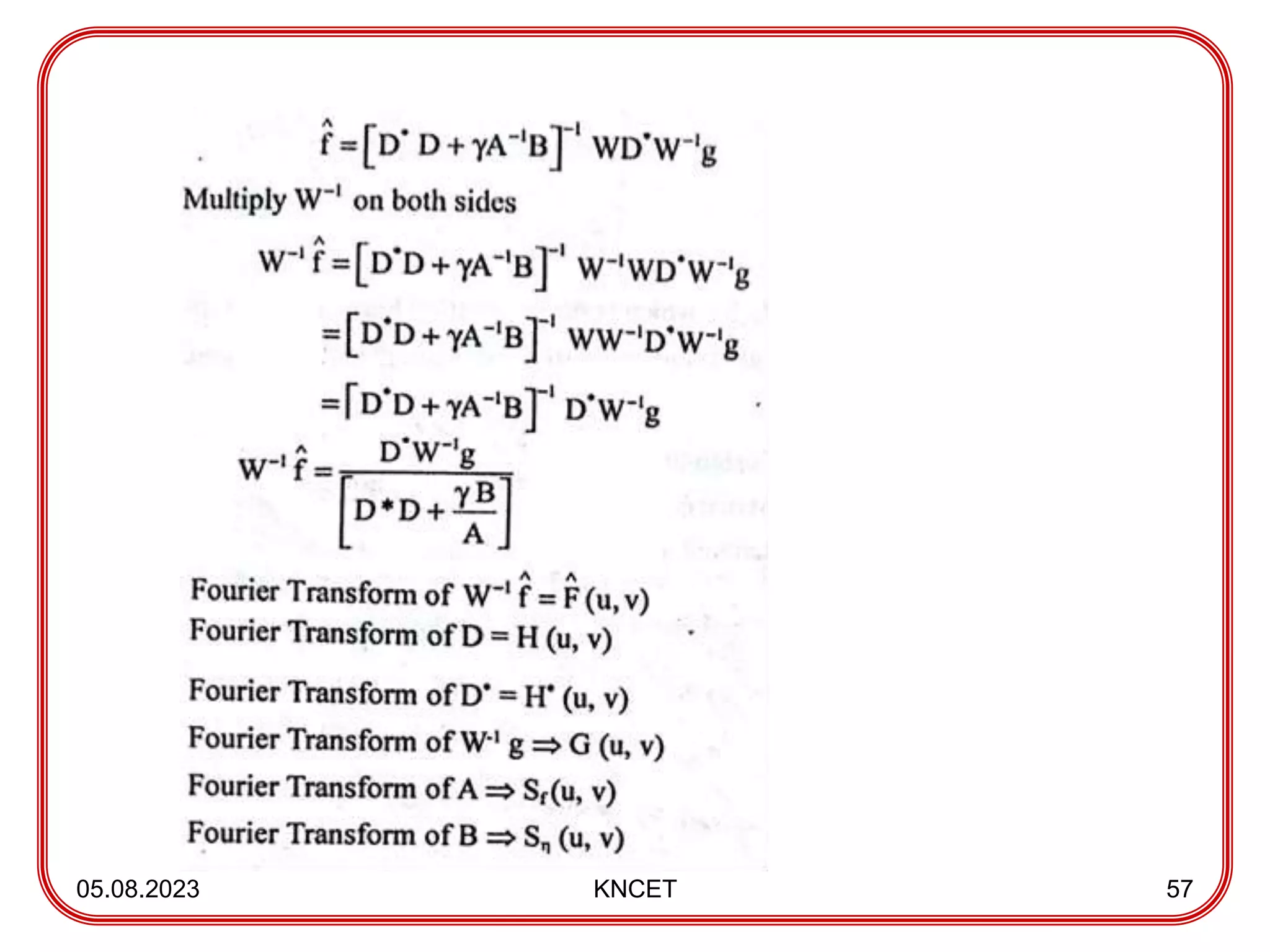
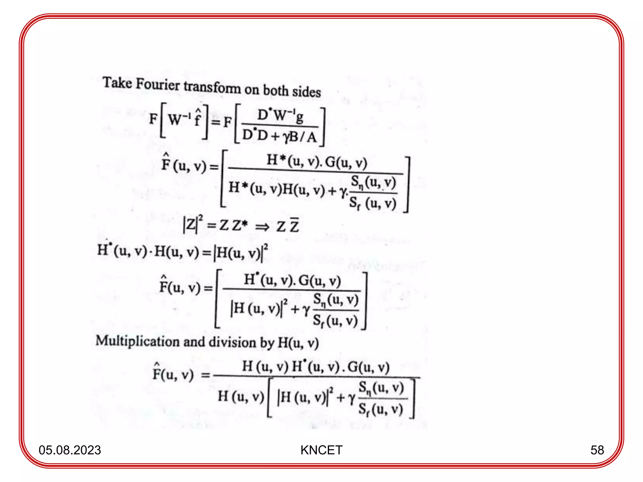
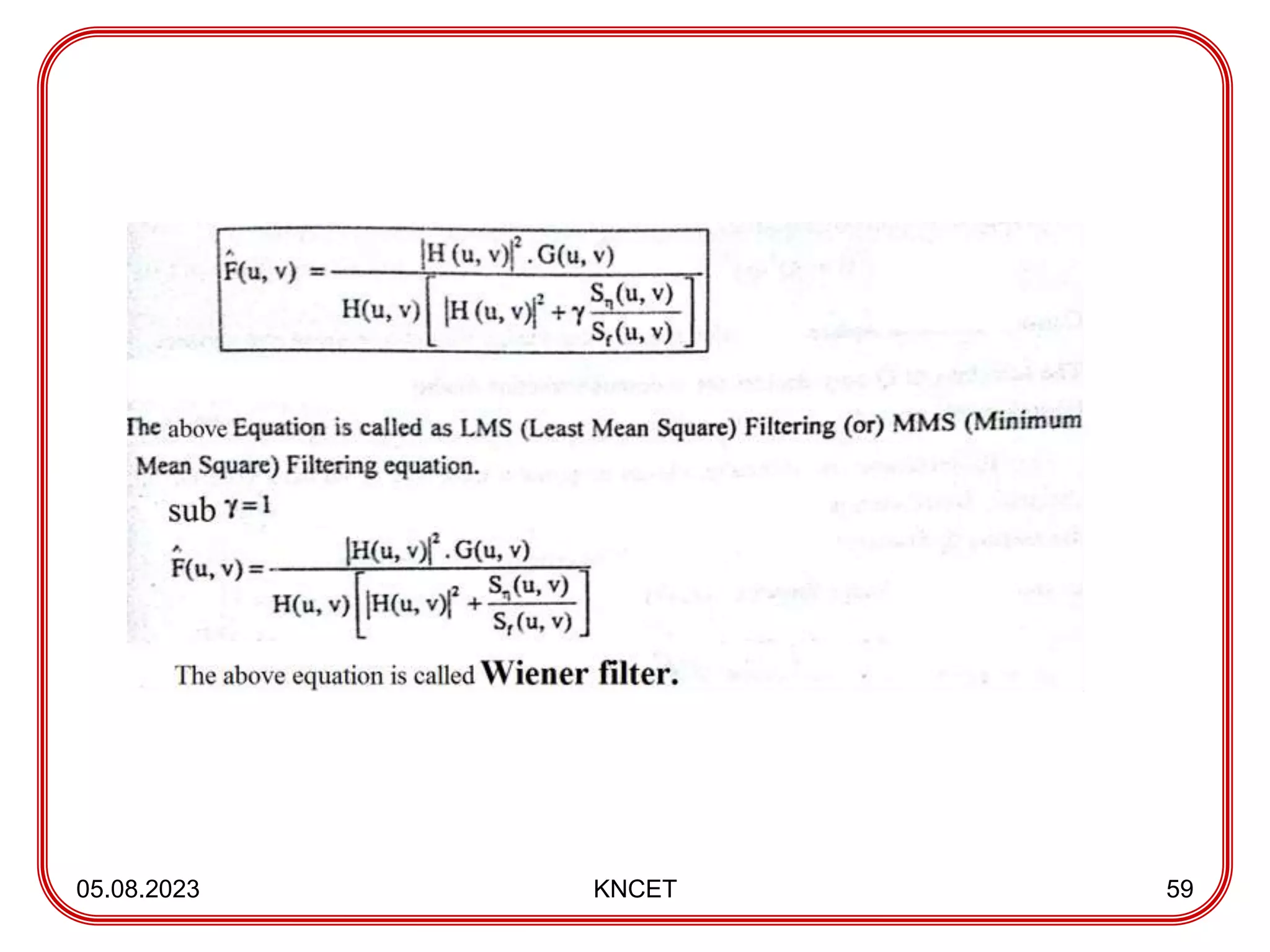
55. Wiener filtering
05.08.2023 KNCET 55
 Wiener filtering is also called as Least Mean Square (LMS) or Minimum Mean Square
(MMS) Filtering.
 Wiener filtering is a method of restoring images in the presence of blur as well as
noise.
 It is used to minimize the mean square error between original image f and
approximated(estimated) image f
ˆ .

56. 05.08.2023 KNCET 56

57. 05.08.2023 KNCET 57

58. 05.08.2023 KNCET 58

59. 05.08.2023 KNCET 59

60. How Wiener filter will become Inverse filter?
05.08.2023 KNCET 60

61. Segmentation
05.08.2023 KNCET 61
 Segmentation is the process of partitioning or dividing the image into its constitute
parts or objects.
 Computer tries to separate objects from the image background.
Example: segmentation of tumor part in MRI brain image.
 In general, autonomous segmentation is one of the most difficult tasks in DIP.
 Segmentation algorithms are based on 2 basic properties namely
1)Discontinuity
2)Similarity

62. Detection of Discontinuities
05.08.2023 KNCET 62
 There are three types of gray level discontinuities
1) Points,
2) Lines
3) Edges.
4) To identify these discontinuities, mask processing is performed,where the response R
of the mask is identified with respect to its center location.

63. 05.08.2023 KNCET 63

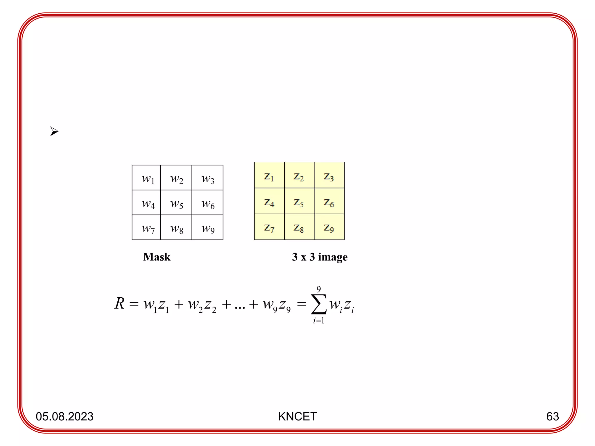
Mask 3 x 3 image
w1 w2 w3
w4 w5 w6
w7 w8 w9







9
1
9
9
2
2
1
1 ...
i
i
i z
w
z
w
z
w
z
w
R

64. Point detection:
05.08.2023 KNCET 64
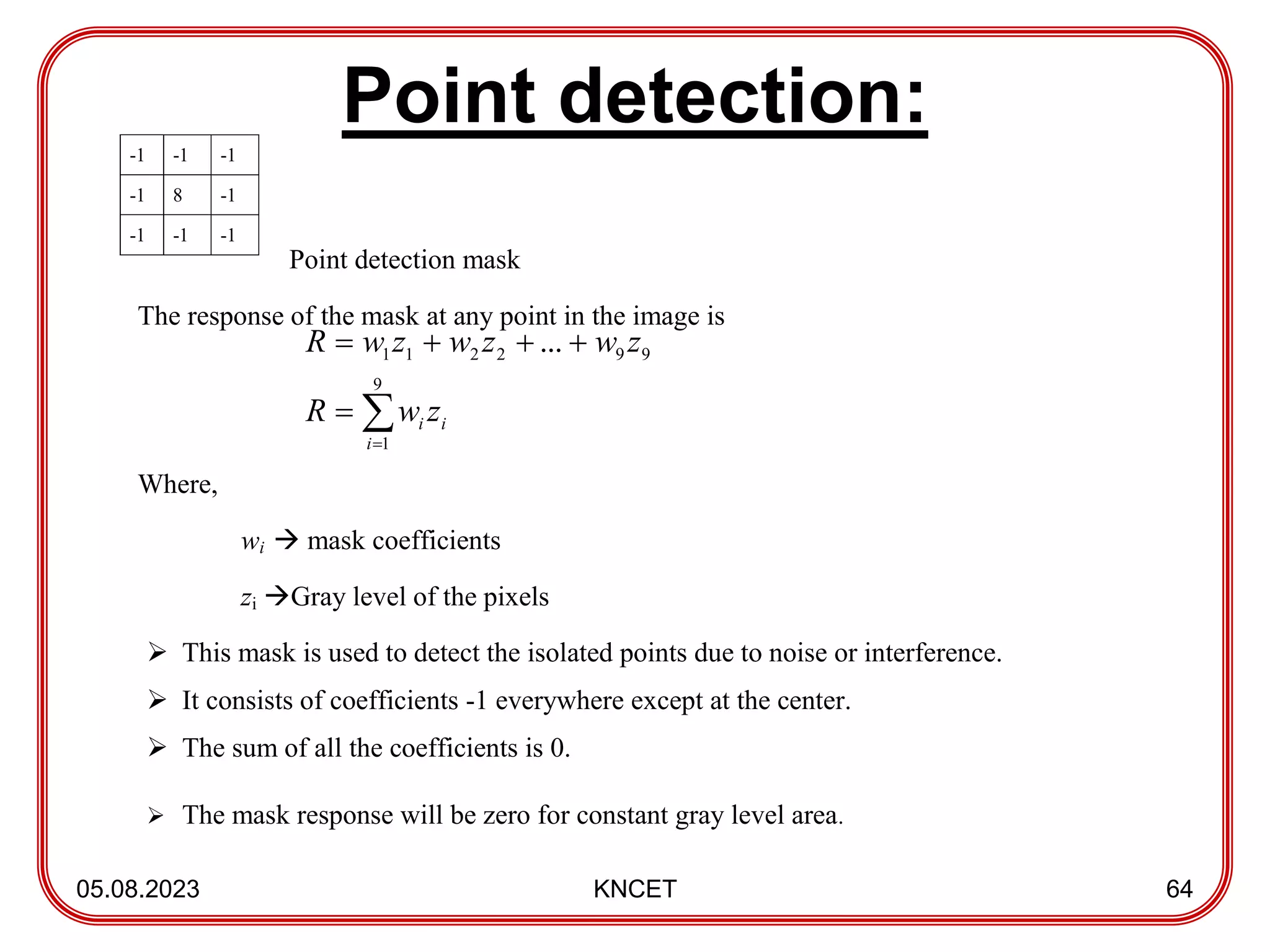
-1 -1 -1
-1 8 -1
-1 -1 -1
Point detection mask
The response of the mask at any point in the image is
Where,
wi  mask coefficients
zi Gray level of the pixels
 This mask is used to detect the isolated points due to noise or interference.
 It consists of coefficients -1 everywhere except at the center.
 The sum of all the coefficients is 0.
 The mask response will be zero for constant gray level area.







9
1
9
9
2
2
1
1 ...
i
i
i z
w
R
z
w
z
w
z
w
R

65. Line detection:
05.08.2023 KNCET 65
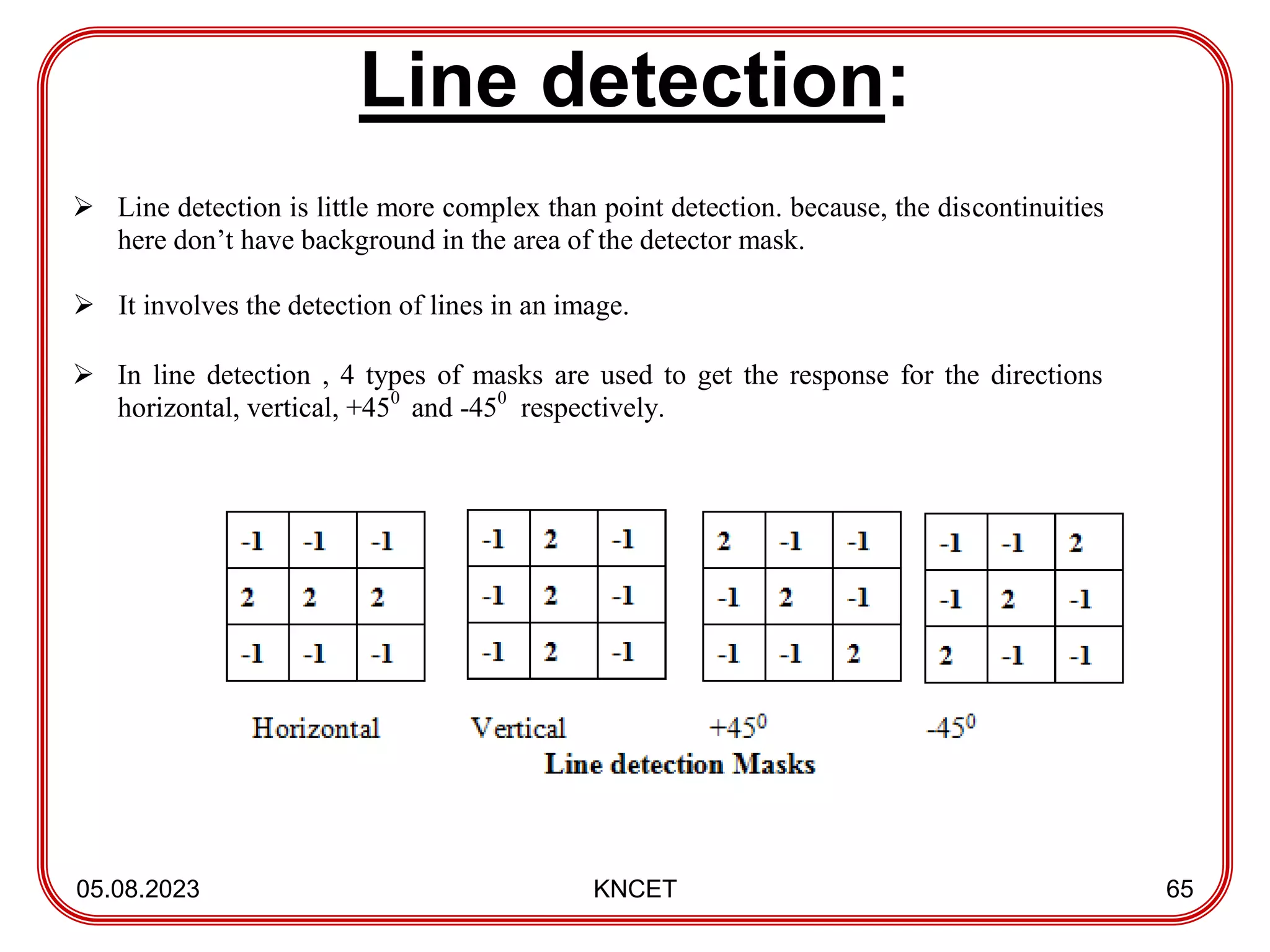
 Line detection is little more complex than point detection. because, the discontinuities
here don’t have background in the area of the detector mask.
 It involves the detection of lines in an image.
 In line detection , 4 types of masks are used to get the response for the directions
horizontal, vertical, +450
and -450
respectively.

66. Edge Detection:
05.08.2023 KNCET 66
 An edge is a set of connected pixels that lie on the boundary between two regions. It
provides an outline or boundary of the object.
 Edge detection is an image processing technique for finding the boundaries of objects
within images. It works by detecting discontinuities in gray level or intensity.

67. 05.08.2023 KNCET 67

68. 05.08.2023 KNCET 68
 The magnitude of first derivative is used to detect the presence of an edge
in an
image.
 The sign of the second derivative is used to find whether the edge pixel lies on the
darkside(or) light side of an edge.
 Second derivative has a zero crossing at the midpoint of the transitions in gray
level.
 The first derivative and second derivative is obtained by using the magnitude of the
gradient and laplacian respectively.

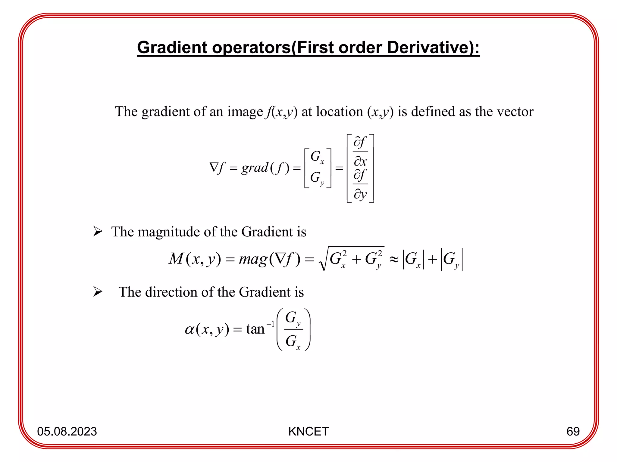
69. Gradient operators(First order Derivative):
05.08.2023 KNCET 69
The gradient of an image f(x,y) at location (x,y) is defined as the vector
 The magnitude of the Gradient is
 The direction of the Gradient is








 
x
y
G
G
y
x 1
tan
)
,
(



























y
f
x
f
G
G
f
grad
f
y
x
)
(
y
x
y
x G
G
G
G
f
mag
y
x
M 




 2
2
)
(
)
,
(

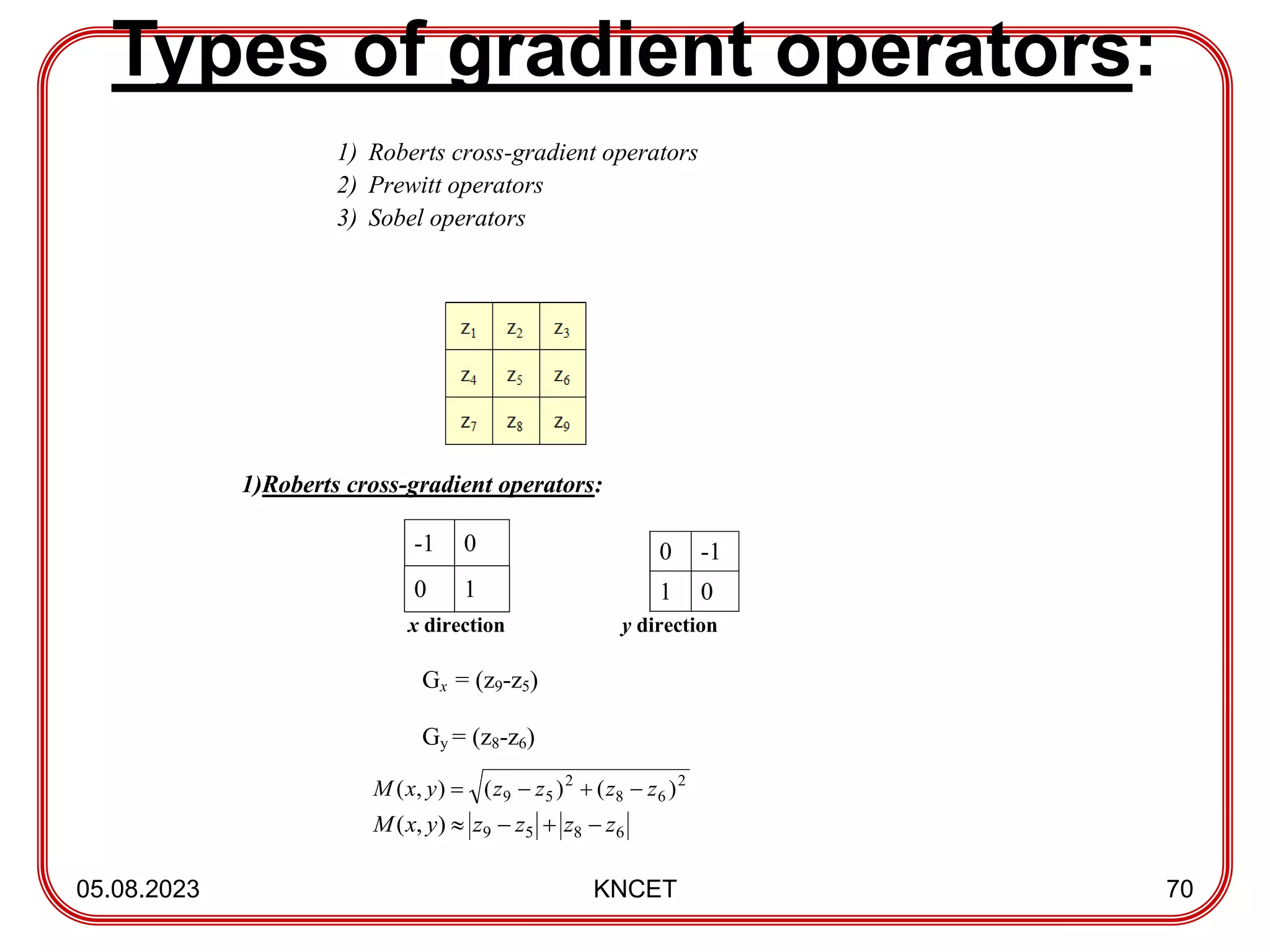
70. Types of gradient operators:
05.08.2023 KNCET 70
1) Roberts cross-gradient operators
2) Prewitt operators
3) Sobel operators
1)Roberts cross-gradient operators:
-1 0
0 1
x direction y direction
Gx = (z9-z5)
Gy = (z8-z6)
0 -1
1 0
6
8
5
9
)
,
( z
z
z
z
y
x
M 



2
6
8
2
5
9 )
(
)
(
)
,
( z
z
z
z
y
x
M 




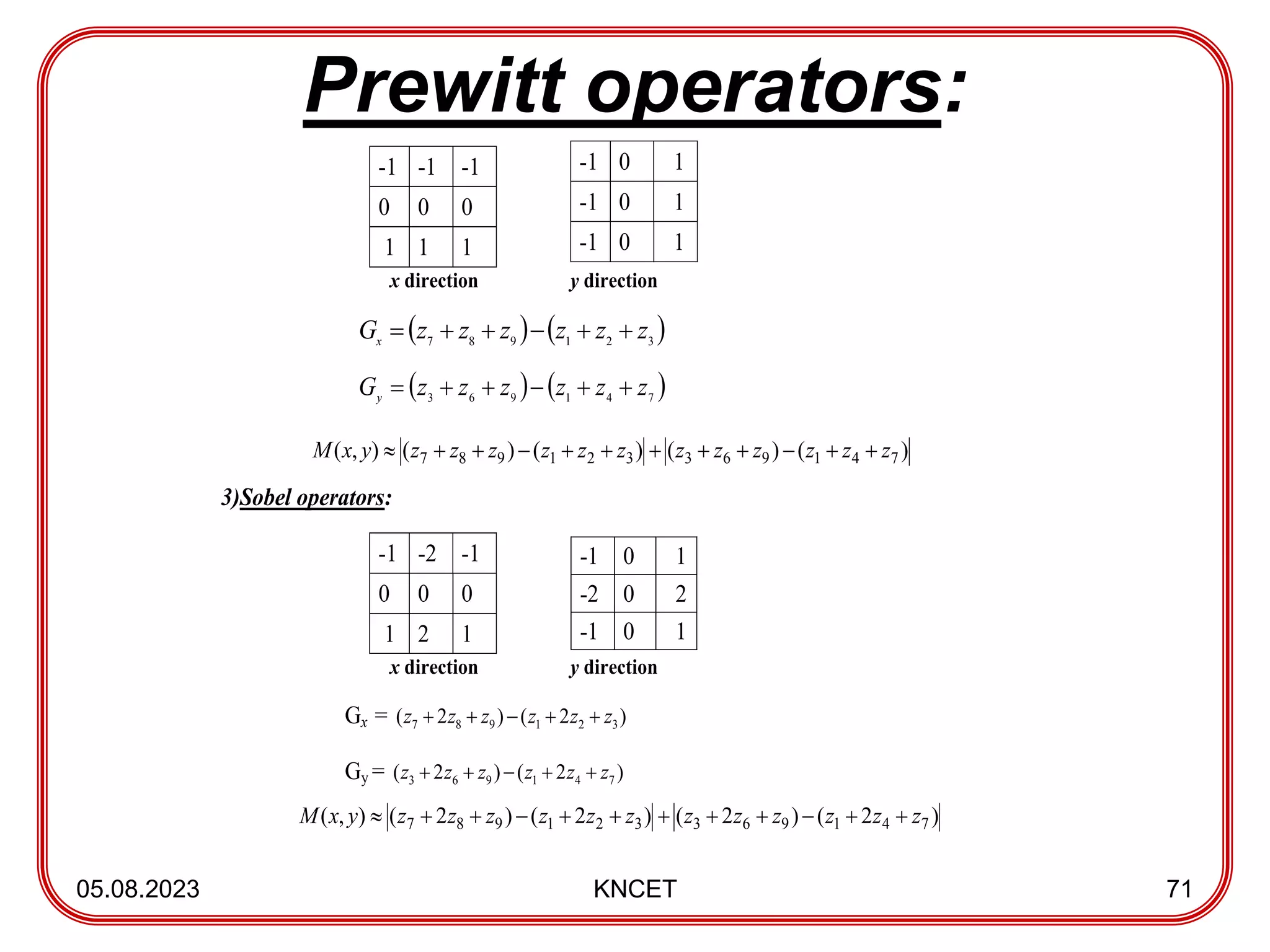
71. Prewitt operators:
05.08.2023 KNCET 71
-1 -1 -1
0 0 0
1 1 1
x direction y direction
   
3
2
1
9
8
7
z
z
z
z
z
z
Gx






   
7
4
1
9
6
3
z
z
z
z
z
z
Gy






3)Sobel operators:
-1 -2 -1
0 0 0
1 2 1
x direction y direction
Gx = )
2
(
)
2
( 3
2
1
9
8
7 z
z
z
z
z
z 




Gy = )
2
(
)
2
( 7
4
1
9
6
3 z
z
z
z
z
z 




-1 0 1
-1 0 1
-1 0 1
-1 0 1
-2 0 2
-1 0 1
)
(
)
(
)
(
)
(
)
,
( 7
4
1
9
6
3
3
2
1
9
8
7 z
z
z
z
z
z
z
z
z
z
z
z
y
x
M 











)
2
(
)
2
(
)
2
(
)
2
(
)
,
( 7
4
1
9
6
3
3
2
1
9
8
7 z
z
z
z
z
z
z
z
z
z
z
z
y
x
M 












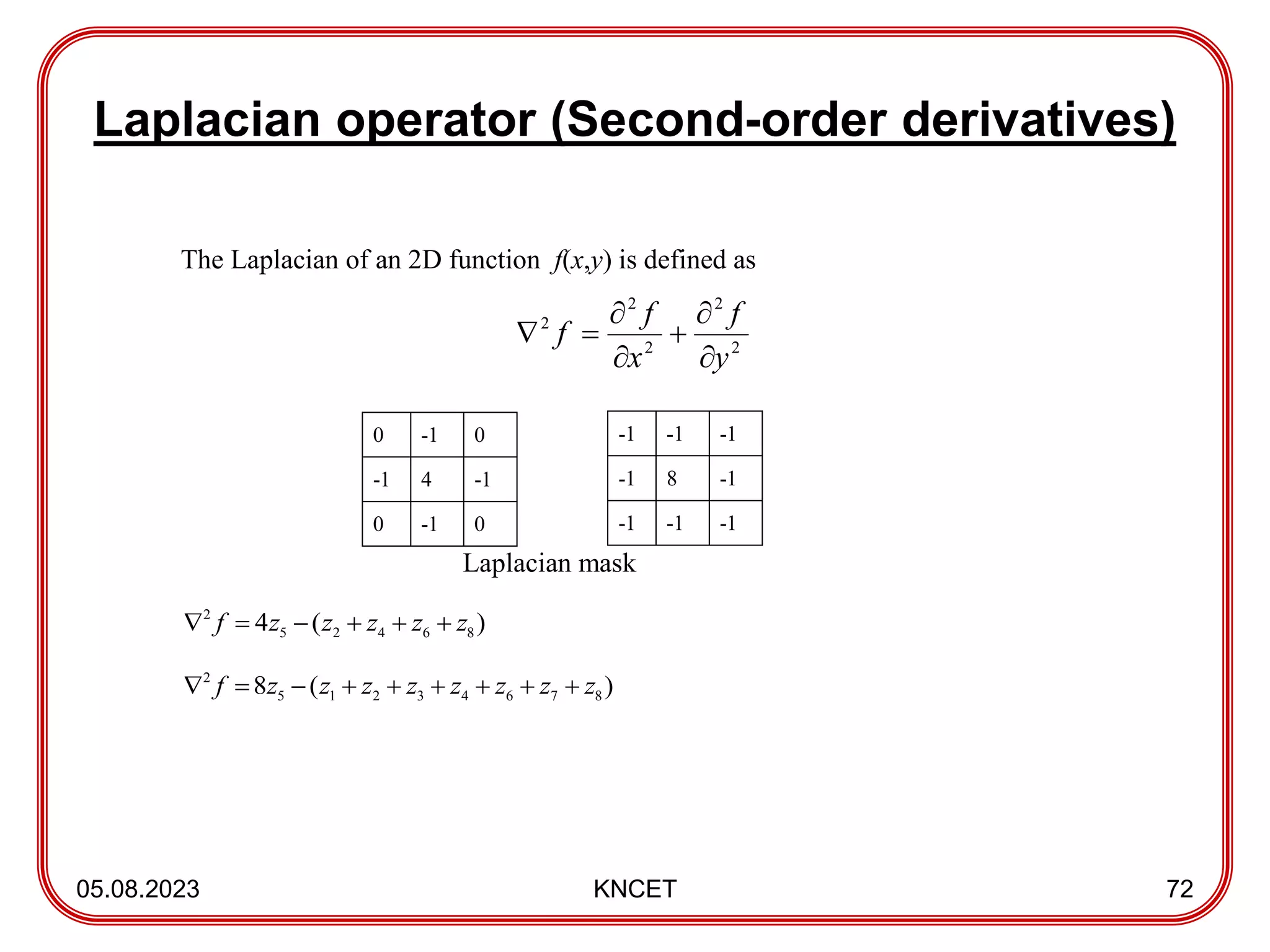
72. Laplacian operator (Second-order derivatives)
05.08.2023 KNCET 72
The Laplacian of an 2D function f(x,y) is defined as
0 -1 0
-1 4 -1
0 -1 0
Laplacian mask
)
(
4 8
6
4
2
5
2
z
z
z
z
z
f 





)
(
8 8
7
6
4
3
2
1
5
2
z
z
z
z
z
z
z
z
f 








-1 -1 -1
-1 8 -1
-1 -1 -1
2
2
2
2
2
y
f
x
f
f








73. Edge Linking and Boundary Detection
05.08.2023 KNCET 73
 An edge is a set of connected pixels that lie on the boundary between two regions.
 Due to noise, non uniform illumination, the pixels does not form a boundary. So
edge linking is required to assemble edge pixels in to meaningful edges.
 Edge linking is the process of connecting the disjoint edges.
Edge linking and boundary detection methods
1) Local processing
2) Regional processing
3) Global processing using Hough transform

74. 05.08.2023 KNCET 74
1) Local processing:
 Local processing is the simplest approach for linking edge points(pixels).
 This is usually done in local neighborhoods.
 Adjacent edge points with similar magnitude and direction are linked.
Two properties used for establishing edge linking:
1) The strength (or magnitude) of the response of the gradient operator used to
produce the edge pixel.
 The direction of the gradient.

75. 05.08.2023 KNCET 75
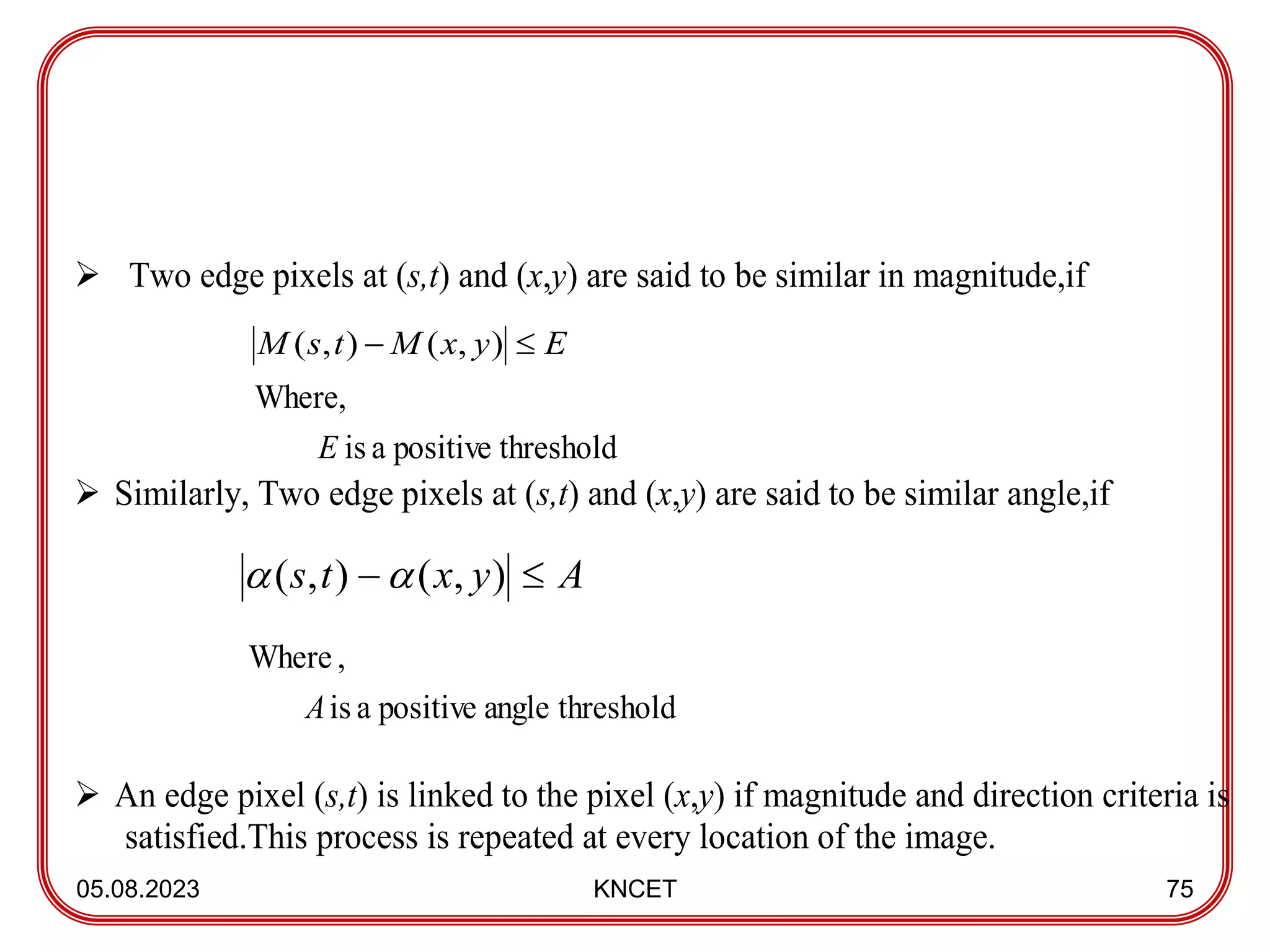
 Two edge pixels at (s,t) and (x,y) are said to be similar in magnitude,if
threshold
positive
a
is
Where,
E
 Similarly, Two edge pixels at (s,t) and (x,y) are said to be similar angle,if
threshold
angle
positive
a
is
,
Where
A
 An edge pixel (s,t) is linked to the pixel (x,y) if magnitude and direction criteria is
satisfied.This process is repeated at every location of the image.
)
,
(
)
,
( E
y
x
M
t
s
M 

)
,
(
)
,
( A
y
x
t
s 



76. 05.08.2023 KNCET 76
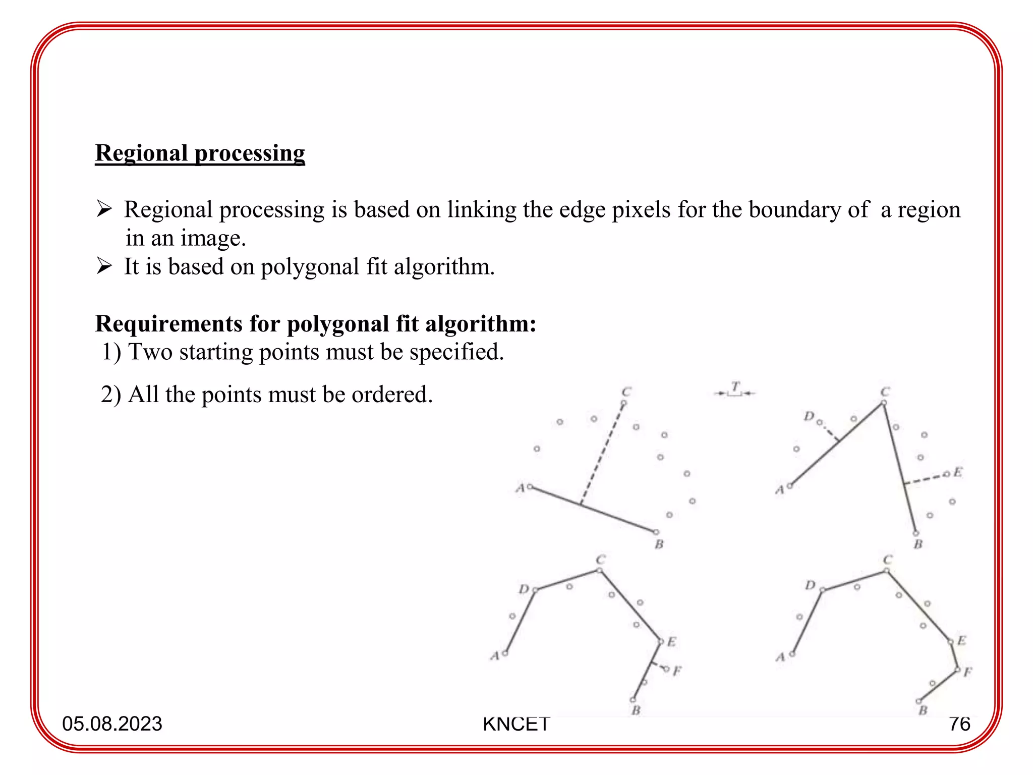
Regional processing
 Regional processing is based on linking the edge pixels for the boundary of a region
in an image.
 It is based on polygonal fit algorithm.
Requirements for polygonal fit algorithm:
1) Two starting points must be specified.
2) All the points must be ordered.

77. 05.08.2023 KNCET 77
Steps:
1. Start with known end points A and B in a binary image.
2. Determine maximum perpendicular distant pixel C from AB.
3. If the distance from AB to C is greater than threshold T pick C as a new endpoint for
new segments AC and CB.
4. Repeat until all perpendicular distances less than T.
3) Global processing using Hough transform:
 The Hough transform is a general technique for identifying the locations and
orientations of certain types of features in a digital image.
 The Hough transform is a technique which can be used to isolate features of a
particular shape within an image.
 It is most commonly used for the detection of regular curves such as lines, circles,
ellipses, etc

78. 05.08.2023 KNCET 78
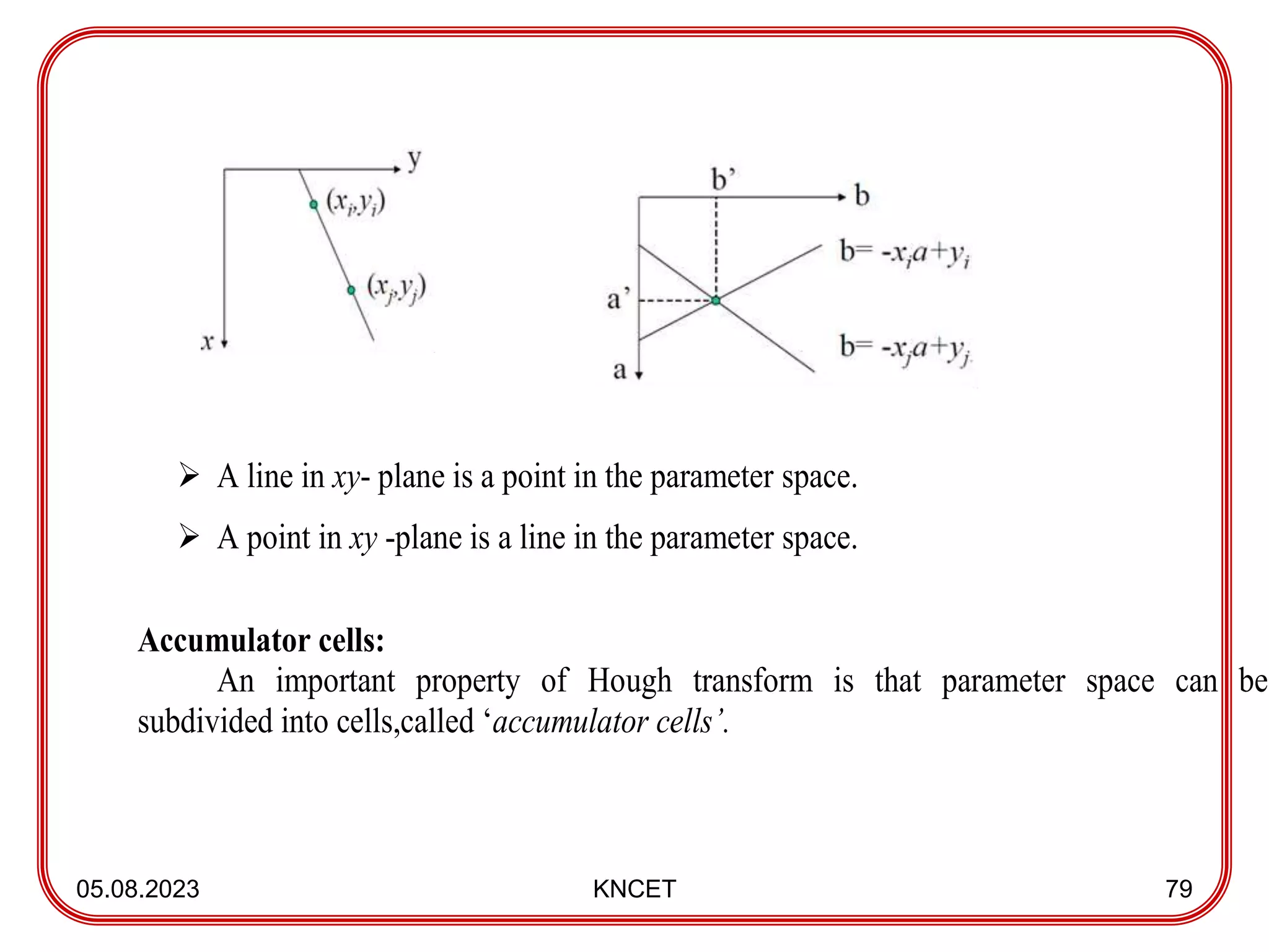
 Consider a point (xi,yi) in the xy -plane and the equation for a straight line
yi=a xi+b
 Infinitely many lines pass through the point (xi,yi), but they all satisfy the equation
yi=a xi+b for varying values of a and b.
 A single line for a fixed pair (xi,yi) in the parameter space or ab- plane can be written as
b=-xia+yi
 Consider a second point (xj,yj) also has a line in the parameter space associated with
it.This line intersects the line associated with (xi,yi) at (a’,b’).
 In fact, all points that lie on this line have corresponding lines in the parameter space
that intersect at (a’,b’)

79. 05.08.2023 KNCET 79
 A line in xy- plane is a point in the parameter space.
 A point in xy -plane is a line in the parameter space.
Accumulator cells:
An important property of Hough transform is that parameter space can be
subdivided into cells,called ‘accumulator cells’.

80. 05.08.2023 KNCET 80
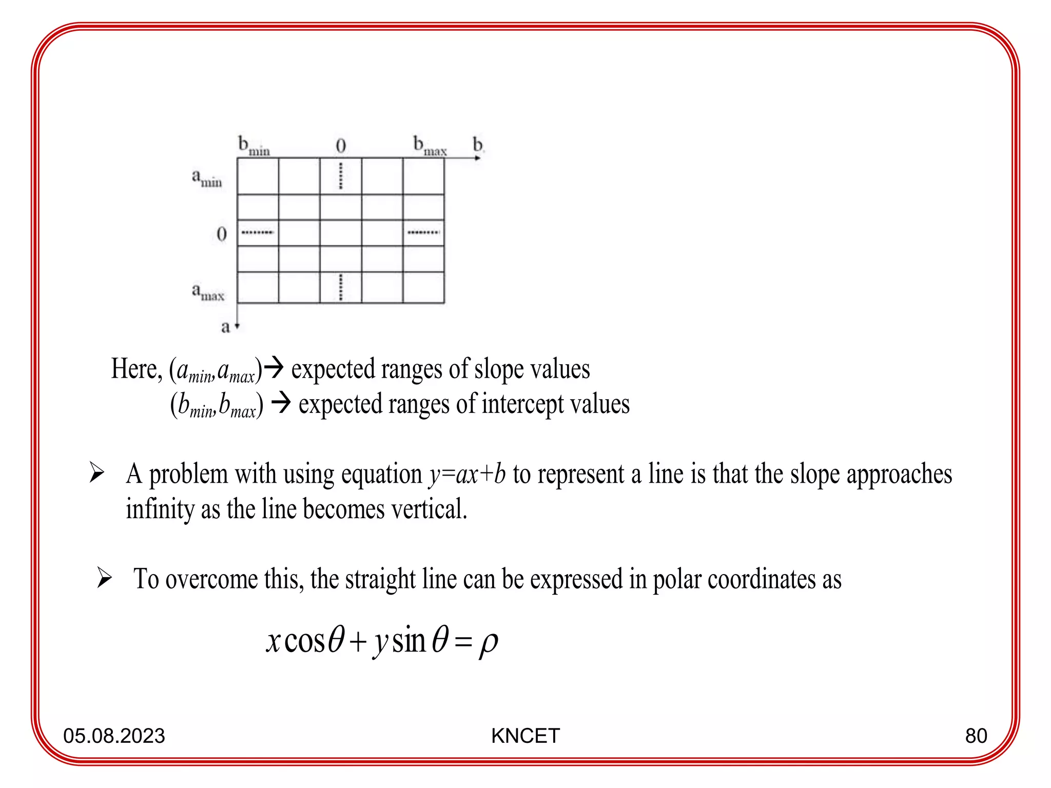
Here, (amin,amax) expected ranges of slope values
(bmin,bmax)  expected ranges of intercept values
 A problem with using equation y=ax+b to represent a line is that the slope approaches
infinity as the line becomes vertical.
 To overcome this, the straight line can be expressed in polar coordinates as


 
 sin
cos y
x

81. 05.08.2023 KNCET 81
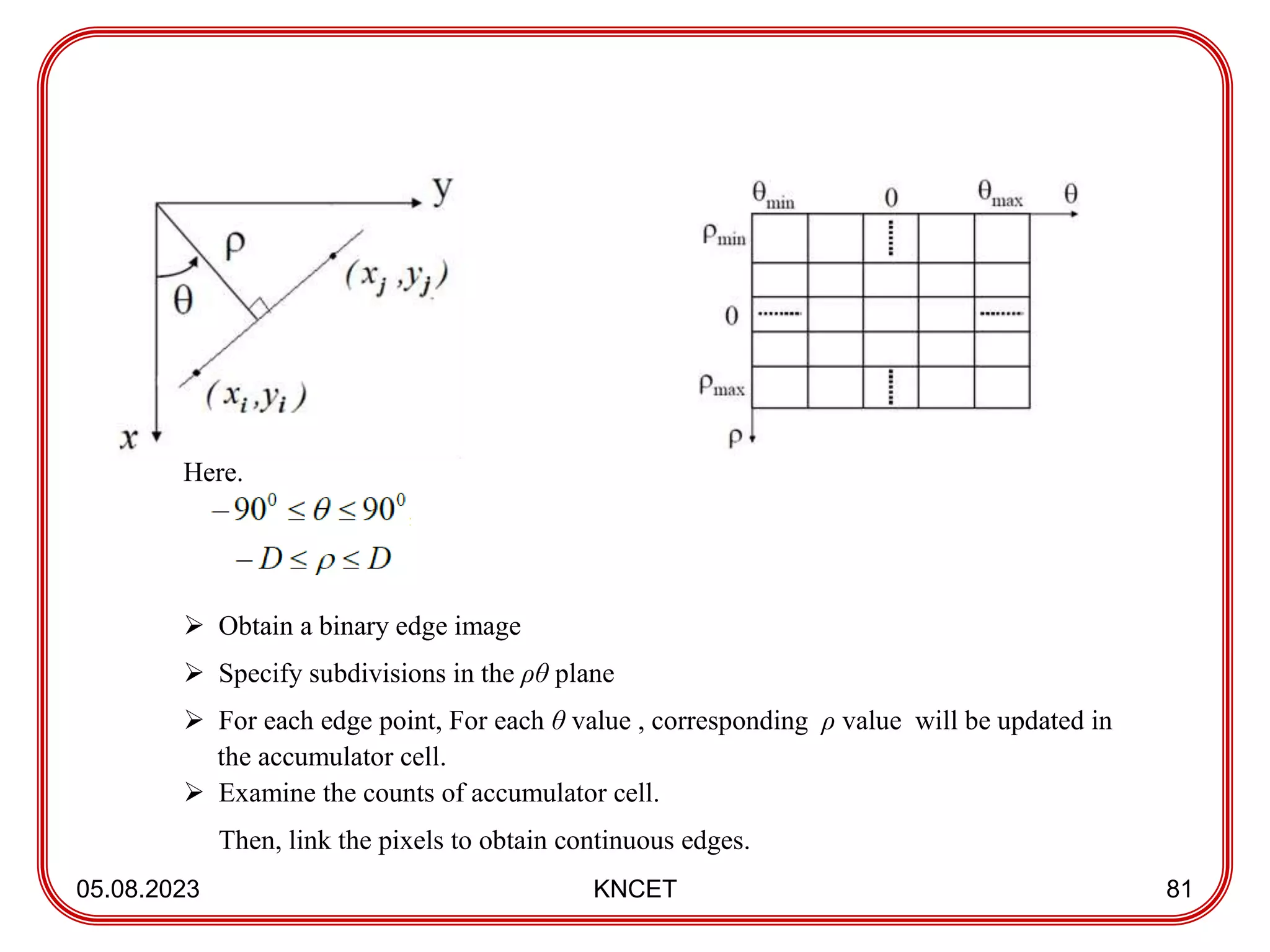
Here.
 Obtain a binary edge image
 Specify subdivisions in the ρθ plane
 For each edge point, For each θ value , corresponding ρ value will be updated in
the accumulator cell.
 Examine the counts of accumulator cell.
 Then, link the pixels to obtain continuous edges.

82. Morphological image processing- Erosion &
Dilation
05.08.2023 KNCET 82
 Morphology is a branch in biology that deals with the structure of animals and
plants.
 Morphological image processing is a tool for extracting image components that deal
with the shape (or morphology) of features in an image.
 Once segmentation is complete, morphological operations can be used to remove
imperfections in the segmented image.
 Usually applied to binary images.
 Using set theory.

83. Basics of Set Theory
05.08.2023 KNCET 83
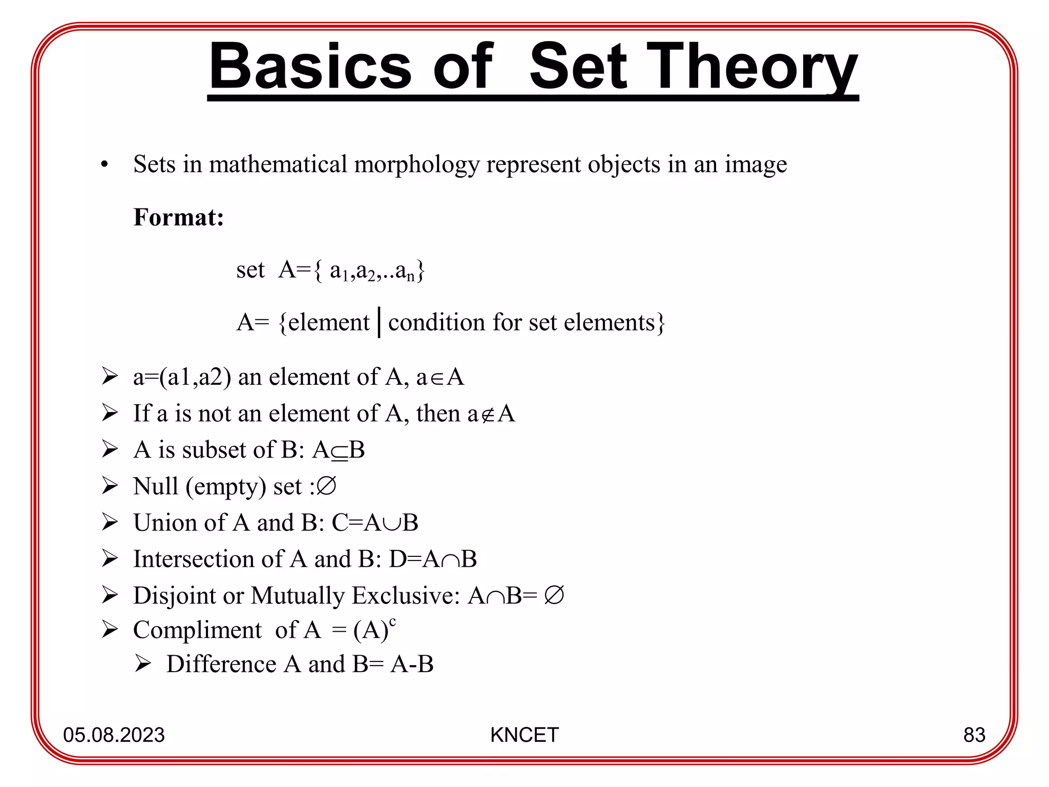
• Sets in mathematical morphology represent objects in an image
Format:
set A={ a1,a2,..an}
A= {element│condition for set elements}
 a=(a1,a2) an element of A, aA
 If a is not an element of A, then aA
 A is subset of B: AB
 Null (empty) set :
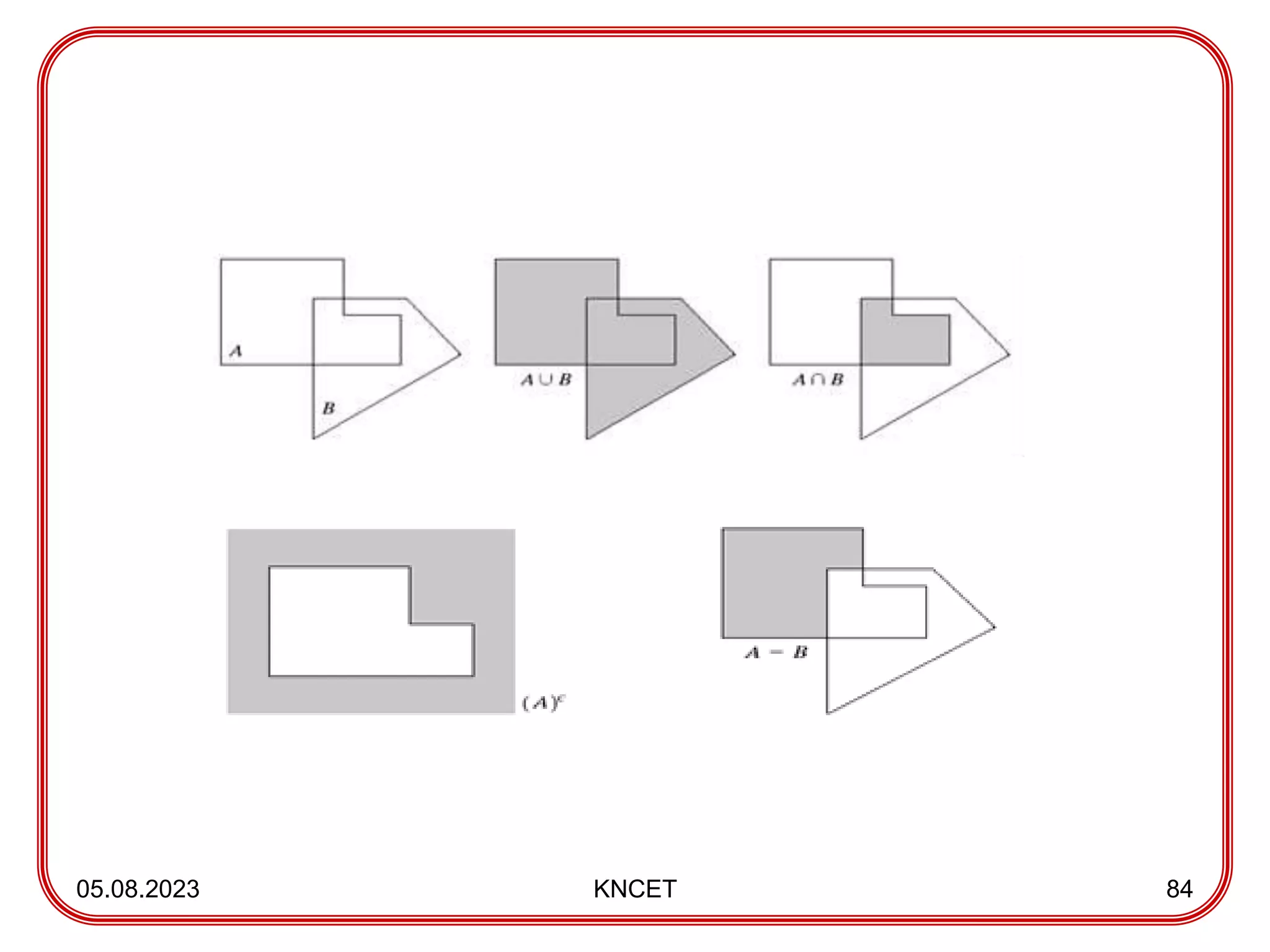
 Union of A and B: C=AB
 Intersection of A and B: D=AB
 Disjoint or Mutually Exclusive: AB= 
 Compliment of A = (A)c
 Difference A and B= A-B

84. 05.08.2023 KNCET 84

85. • The two basic morphological operations:
• Erosion
• Dilation
05.08.2023 KNCET 85
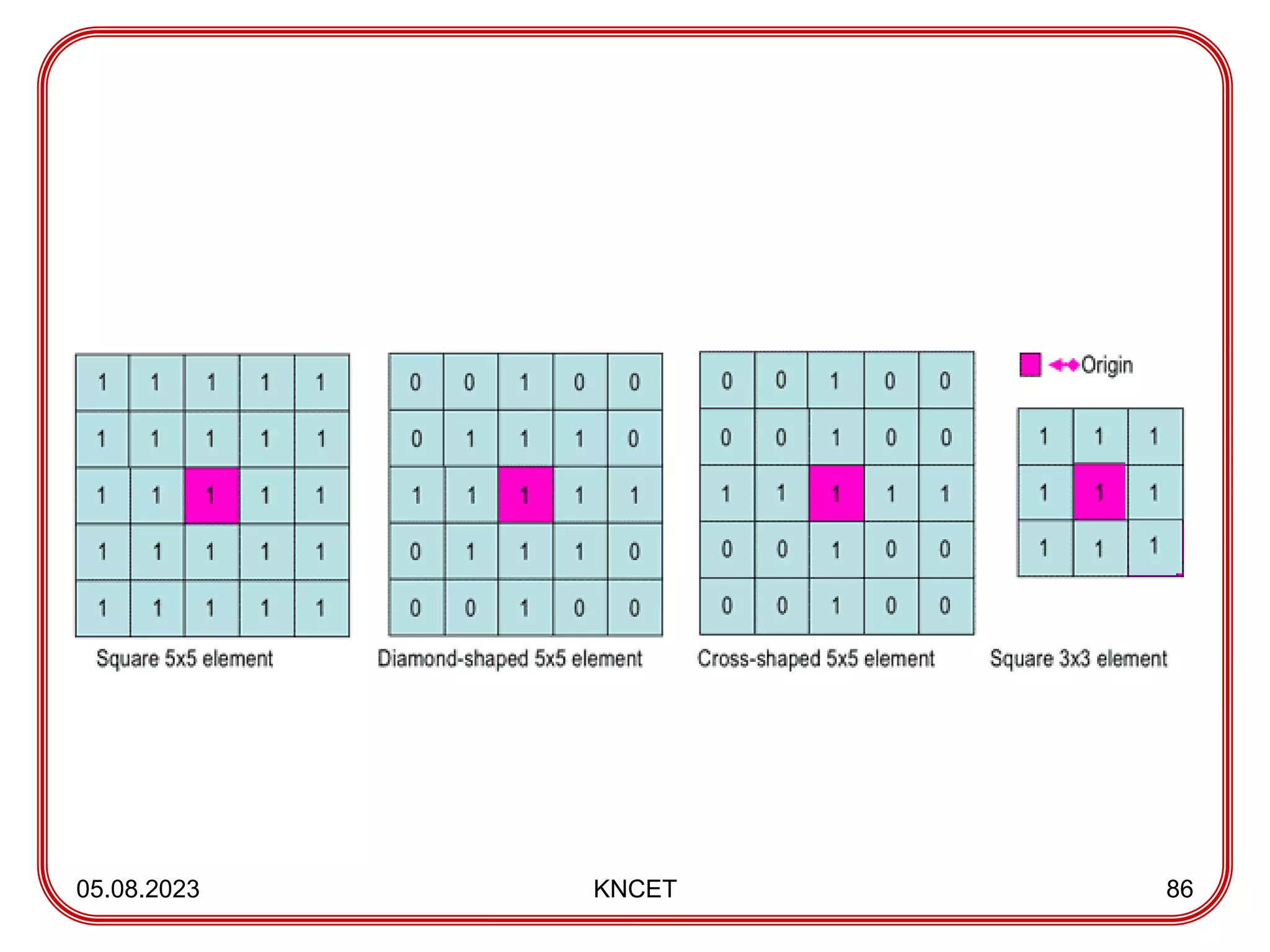
Structuring Elements
 A structuring element is a shape mask used in the basic morphological
operations.
 Structuring elements can be any shape and size.
 It generally consists of matrix of 0’s and 1’s.
 Structural Elements have an origin, generally at the center pixel.
Fit: All pixels in the structuring element cover on pixels in the image
Hit: Any one pixel in the structuring element covers an on pixel in the image.

86. 05.08.2023 KNCET 86

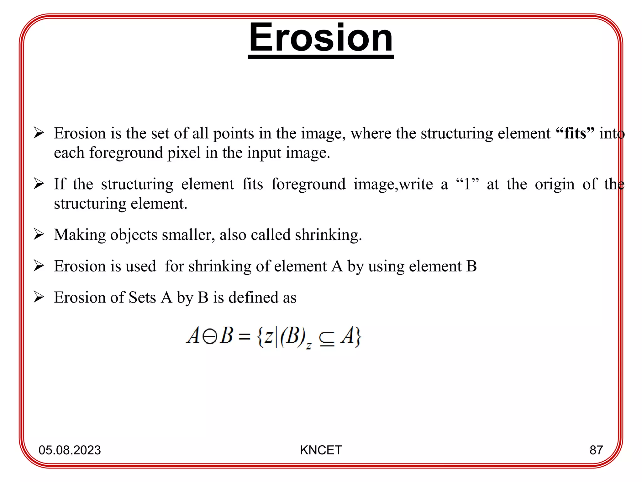
87. Erosion
05.08.2023 KNCET 87
 Erosion is the set of all points in the image, where the structuring element “fits” into
each foreground pixel in the input image.
 If the structuring element fits foreground image,write a “1” at the origin of the
structuring element.
 Making objects smaller, also called shrinking.
 Erosion is used for shrinking of element A by using element B
 Erosion of Sets A by B is defined as

88. Example:
05.08.2023 KNCET 88

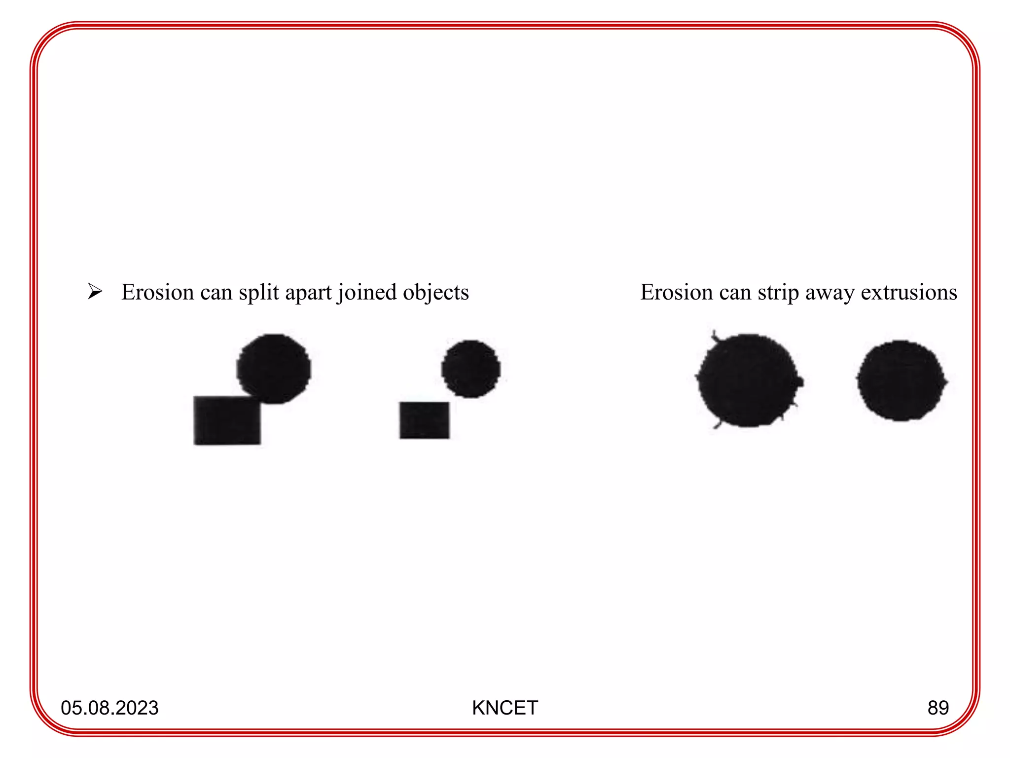
89. 05.08.2023 KNCET 89
 Erosion can split apart joined objects Erosion can strip away extrusions

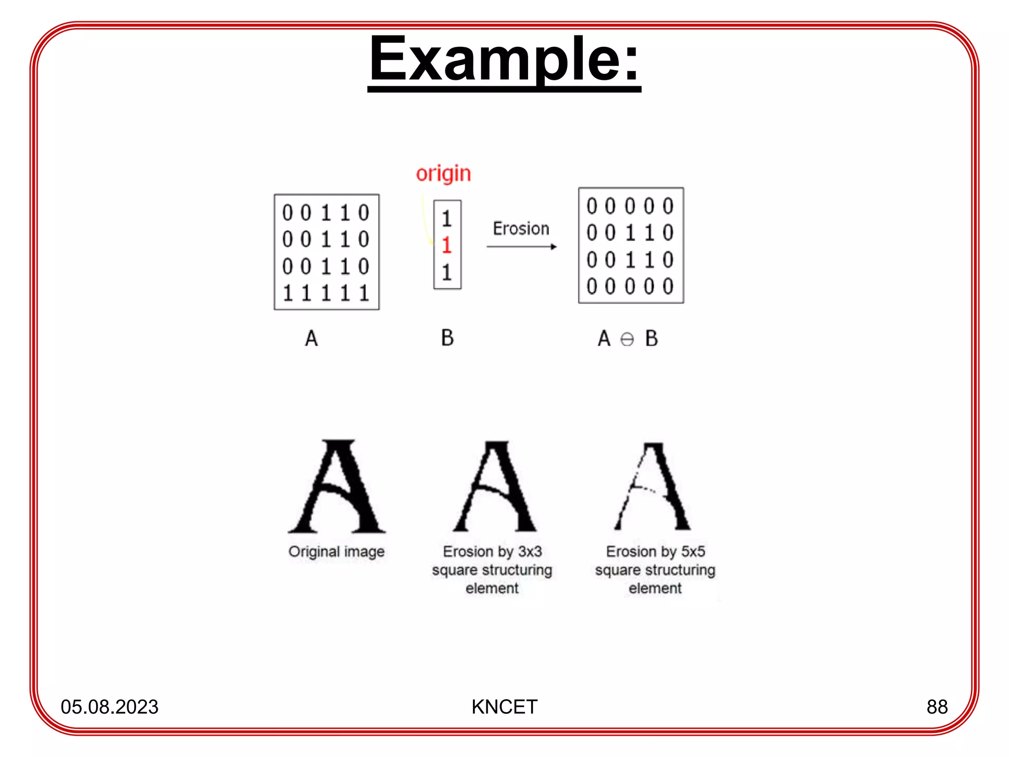
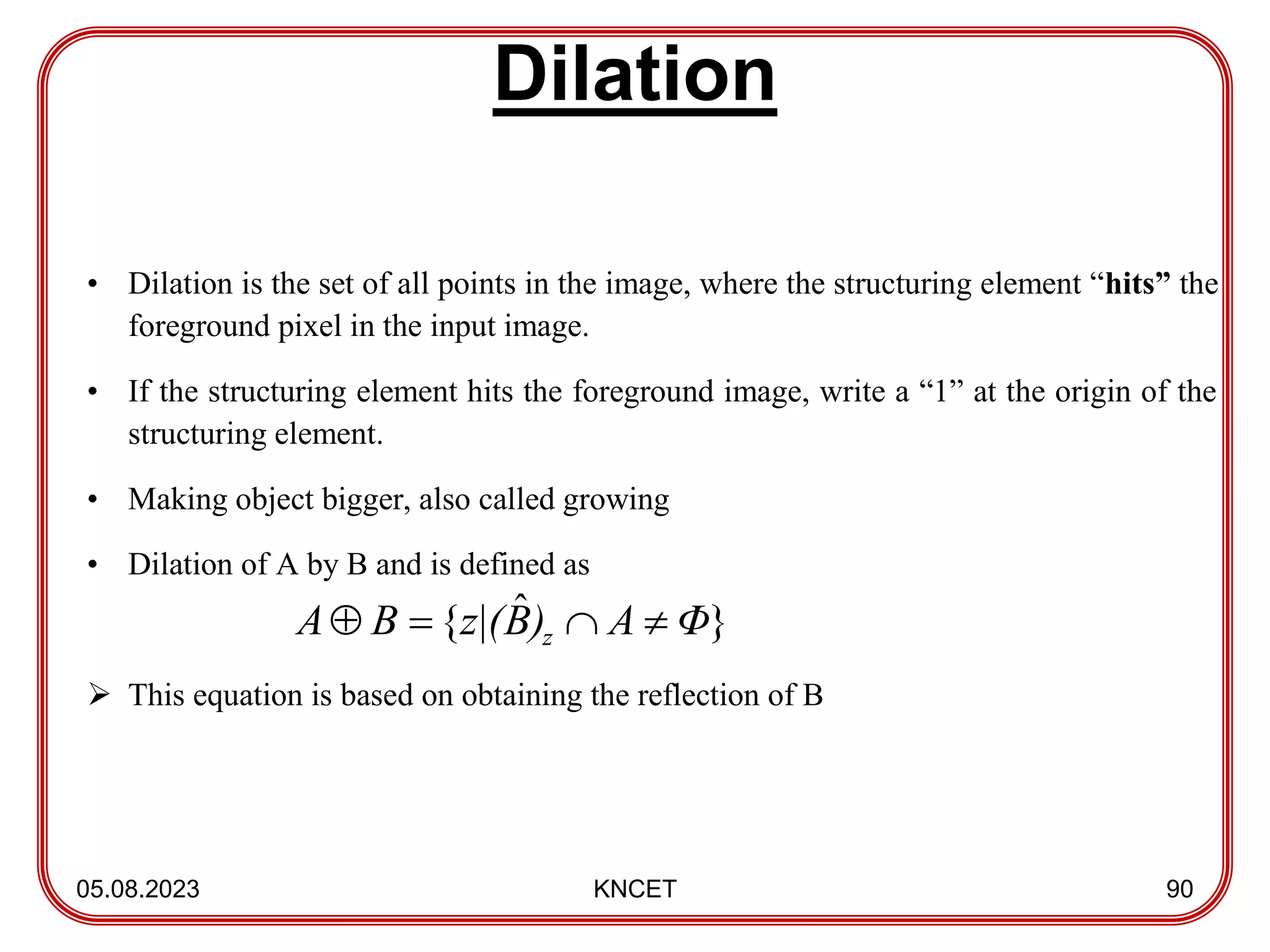
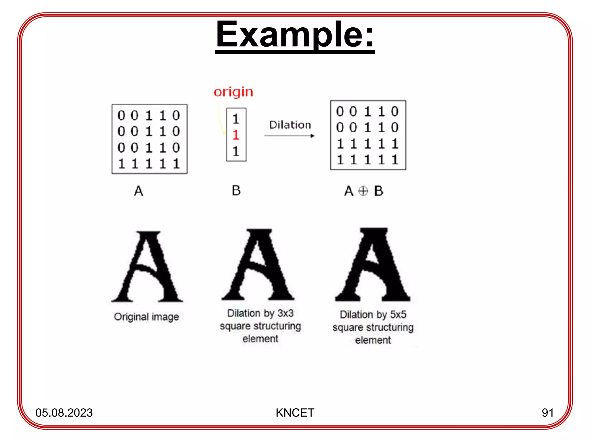
90. Dilation
05.08.2023 KNCET 90
• Dilation is the set of all points in the image, where the structuring element “hits” the
foreground pixel in the input image.
• If the structuring element hits the foreground image, write a “1” at the origin of the
structuring element.
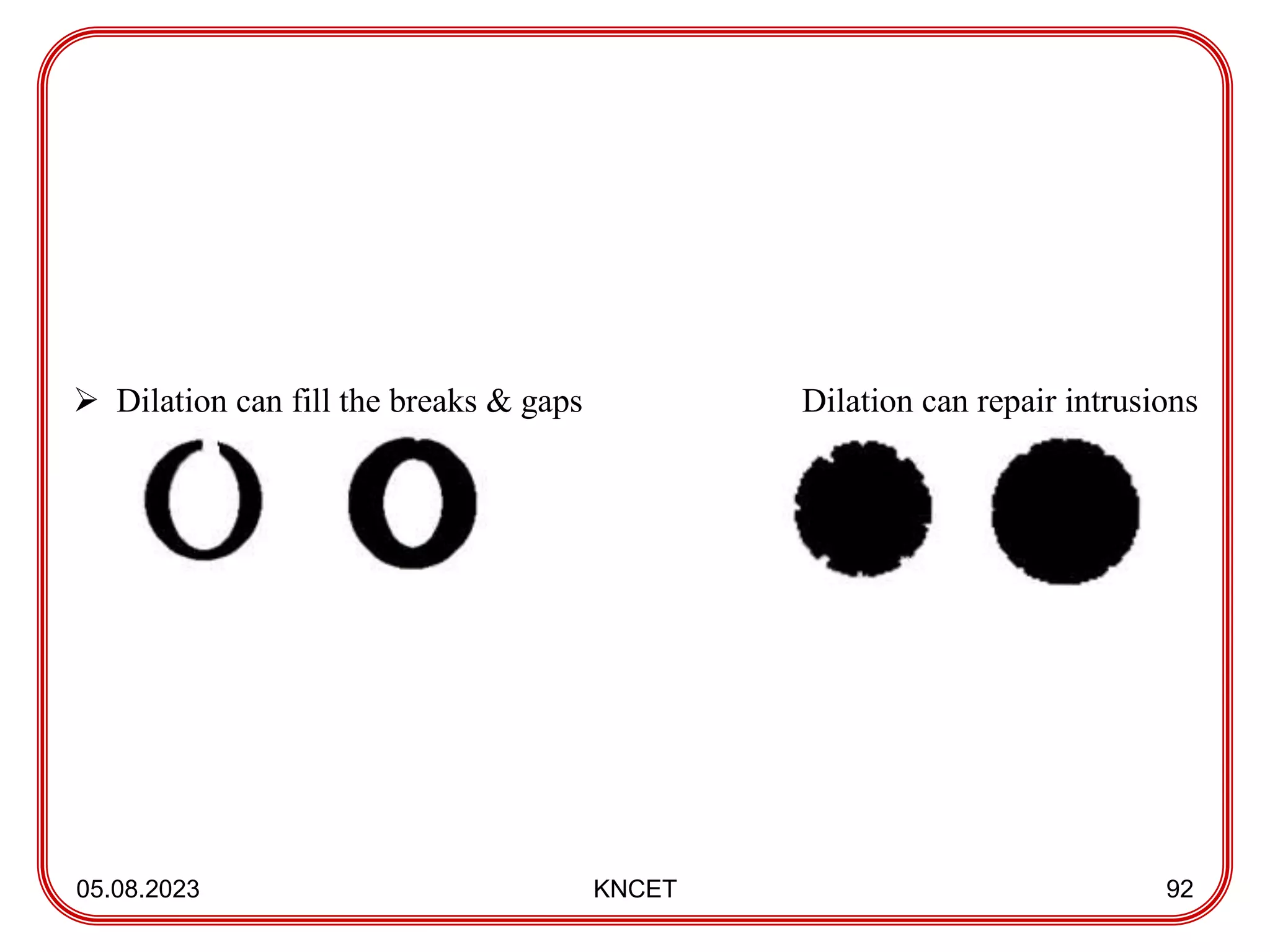
• Making object bigger, also called growing
• Dilation of A by B and is defined as
 This equation is based on obtaining the reflection of B
}
ˆ
{ Φ
A
)
B
z|(
B
A z 




91. Example:
05.08.2023 KNCET 91

92. 05.08.2023 KNCET 92
 Dilation can fill the breaks & gaps Dilation can repair intrusions