This document discusses theorems related to linear transformations between finite-dimensional vector spaces. It proves two main theorems: 1) A linear transformation T is invertible if and only if T maps a basis of the domain space V to a basis of the codomain space W. 2) A linear transformation T between vector spaces of equal dimension is invertible, injective, surjective, and maps bases to bases. These properties are shown to be equivalent. The document provides a detailed proof of each theorem with examples to illustrate the concepts. It discusses key ideas such as linear independence, spanning sets, and the relationship between invertibility, injectivity and surjectivity of linear transformations.

1. CAPÍTULO III
MATRIZ ASOCIADA A UNA TRANSFORMACIÓN LINEAL.
CONTENIDO:
3.1 Matriz asociada a una transformación lineal.
3.2 Algebra de transformaciones lineales.
3.3 Composición de Transformaciones lineales.
3.4 Transformaciones lineales invertibles.
3.5 Teorema de equivalencias de una transformación lineal.
3.6 Isomorfismo inducido por una transformación lineal.
3.7 Cambio de base y semejanza de matrices.
3.8 Producto Interno. Definición. Teoremas de caracterización.
3.9 Norma de un Vector.
3.10 Ortogonalidad. Conjunto ortogonal y conjunto ortonormal.
3.11 Proceso de ortogonalidad de Gram Schmitdt.
3.12 Espacio Dual de un espacio vectorial.
3.13 Adjunta de una transformación lineal

2. 88
3.5 TEOREMAS DE EQUIVALENCIAS DE UNA TRANSFORMACIÓN LINEAL.
TEOREMA 1.Sean (𝑉; 𝐾; +; ∙),(𝑊;𝐾;+; ∙) espaciosvectoriales de dimensión finitay 𝑇:𝑉 → 𝑊
una transformaciónlineal entonces, 𝑇 es invertible  𝑇 transforma una base de 𝑉 en una base
de 𝑊.
Demostración.
() Si 𝑇 es invertible  𝑇 transforma una base de 𝑉 en una base de 𝑊. ¡Probar!
Sea [𝑣] = {𝑣1;𝑣2;…; 𝑣𝑛} una base de 𝑉 y sean 𝑤1 = 𝑇(𝑣1); 𝑤2 = 𝑇(𝑣2);…; 𝑤𝑛 = 𝑇(𝑣𝑛) sus
imágenes.
Es decir {𝑤1;𝑤2;… ;𝑤𝑛}es una base de 𝑊. ¡Probar!
(i) El conjunto {𝑤1;𝑤2;…; 𝑤𝑛}es linealmente independiente.
Sea 𝑐1𝑤1 + 𝑐2𝑤2 + ⋯+ 𝑐𝑛𝑤𝑛 = 0𝑊  𝑐1 = 𝑐2 = ⋯ = 𝑐𝑛 = 0 ¡Probar!
Aplicando 𝑇−1, dado que 𝑇 es invertible y además es una transformación lineal:
𝑇−1(𝑐1𝑤1 + 𝑐2𝑤2 + ⋯+ 𝑐𝑛𝑤𝑛) = 𝑇−1(0𝑊)
 𝑐1𝑇−1(𝑤1) + 𝑐2𝑇−1(𝑤2) + ⋯+ 𝑐𝑛𝑇−1(𝑤𝑛) = 𝑇−1(0𝑊)
 𝑐1𝑣1 + 𝑐2𝑣2 + ⋯+ 𝑐𝑛𝑣𝑛 = 0𝑉 y como {𝑣1;𝑣2;… ;𝑣𝑛}es una base de 𝑉
 𝑐1 = 𝑐2 = ⋯ = 𝑐𝑛 = 0
Por lo tanto, el conjunto {𝑤1;𝑤2;… ;𝑤𝑛}es linealmente independiente.
(ii) El conjunto [𝑤] = {𝑤1;𝑤2;…;𝑤𝑛} genera al espacio 𝑊, es decir 𝐿{[𝑤]} = 𝑊
Sea cualquiera 𝑤 ∈ 𝑊  𝑇−1(𝑤) = 𝑣 ∈ 𝑉  𝑇−1(𝑤) = 𝑐1𝑣1 + 𝑐2𝑣2 + ⋯+ 𝑐𝑛𝑣𝑛
Aplicando 𝑇: 𝑇[𝑇−1(𝑤)] = 𝑇(𝑐1𝑣1 + 𝑐2𝑣2 + ⋯+ 𝑐𝑛𝑣𝑛)
 𝑤 = 𝑇(𝑐1𝑣1 + 𝑐2𝑣2 + ⋯+ 𝑐𝑛𝑣𝑛) = 𝑐1𝑇(𝑣1) + 𝑐2𝑇(𝑣2) + ⋯+ 𝑐𝑛𝑇(𝑣𝑛)
 𝑤 = 𝑐1𝑤1 + 𝑐2𝑤2 + ⋯+ 𝑐𝑛𝑤𝑛 (a 𝑤 se le puede escribir en C. L. de la base [𝑤])
Por lo tanto, {𝑤1;𝑤2;… ;𝑤𝑛}genera al espacio 𝑊.
De (i) y (ii) el conjunto {𝑤1;𝑤2;…; 𝑤𝑛}es una base de 𝑊.
() Si 𝑇 transforma una base de 𝑉 en una base de 𝑊  𝑇 es invertible ¡Probar!

3. 89
(Es decir, debe existir 𝑇−1:𝑊 → 𝑉 tal que 𝑇−1𝑜𝑇 = 𝐼𝑉 y 𝑇𝑜𝑇−1 = 𝐼𝑊) ¡Probar!
Defínase la transformación lineal 𝐹:𝑊 → 𝑉 tal que 𝐹(𝑤𝑖) = 𝑣𝑖, ∀ 𝑖 = 1;2; …;𝑛 por el teorema
fundamental de las transformaciones lineales.
i) Probar que 𝐹𝑜𝑇 = 𝐼𝑉 .
Sea 𝑣 ∈ 𝑉  𝑣 = 𝑐1𝑣1 + 𝑐2𝑣2 + ⋯+ 𝑐𝑛𝑣𝑛
 (𝐹𝑜𝑇)(𝑣) = 𝐹[𝑇(𝑣)] =𝐹[𝑇(𝑐1𝑣1 + 𝑐2𝑣2 + ⋯+ 𝑐𝑛𝑣𝑛)]
= 𝐹[𝑐1𝑇(𝑣1) + 𝑐2𝑇(𝑣2)+ ⋯+ 𝑐𝑛𝑇(𝑣𝑛)]pues 𝑇 es transformación lineal.
= 𝐹(𝑐1𝑤1 + 𝑐2𝑤2 + ⋯+ 𝑐𝑛𝑤𝑛)
= 𝑐1𝐹(𝑤1) + 𝑐2𝐹(𝑤2)+ ⋯+ 𝑐𝑛𝐹(𝑤𝑛)pues 𝐹 es transformación lineal.
= 𝑐1𝑣1 + 𝑐2𝑣2 + ⋯+ 𝑐𝑛𝑣𝑛 = 𝑣 ∈ 𝑉  (𝐹𝑜𝑇)(𝑣) = 𝑣 = 𝐼(𝑣)
 𝐹 𝑜 𝑇 = 𝐼𝑉 es la identidad en el espacio vectorial 𝑉.
ii) Probar que 𝑇𝑜𝐹 = 𝐼𝑊.
Sea 𝑤 ∈ 𝑊  𝑤 = 𝑐1𝑤1 + 𝑐2𝑤2 + ⋯+ 𝑐𝑛𝑤𝑛
 (𝑇𝑜𝐹)(𝑤) = 𝑇[𝐹(𝑤)]=𝑇[𝐹(𝑐1𝑤1 + 𝑐2𝑤2 + ⋯+ 𝑐𝑛𝑤𝑛)]
= 𝑇[𝑐1𝐹(𝑤1) + 𝑐2𝐹(𝑤2)+ ⋯+ 𝑐𝑛𝐹(𝑤𝑛)]pues 𝐹 es una transformación lineal.
= 𝑇(𝑐1𝑣1 + 𝑐2𝑣2 + ⋯+ 𝑐𝑛𝑣𝑛)
= 𝑐1𝑇(𝑣1) + 𝑐2𝑇(𝑣2)+ ⋯+ 𝑐𝑛𝑇(𝑣𝑛)pues 𝑇 es una transformación lineal.
= 𝑐1𝑤1 + 𝑐2𝑤2 + ⋯+ 𝑐𝑛𝑤𝑛 = 𝑤 ∈ 𝑊  (𝑇𝑜𝐹)(𝑤) = 𝑤 = 𝐼(𝑤)
 𝑇 𝑜 𝐹 = 𝐼𝑊 es la identidad en el espacio vectorial 𝑊.
Luego de (i) y (ii) 𝑇 es invertible siendo la transformación lineal 𝐹 su inversa.
Es decir: 𝐹 = 𝑇−1.
Por lo tanto , de () y () el teorema queda demostrado.
EJEMPLO. Sea la transformación lineal 𝑇: 𝑅2 → 𝑃≤1definida por 𝑇(𝑎; 𝑏) = 2𝑎 − 𝑏𝑥, y sea [𝑣] =
{(1;−1); (2;3)} dos vectores de 𝑅2.
a) Mostrar que [𝑣] = {(1;−1);(2;3)} una base de 𝑅2.

4. 90
b) Mostrar que 𝑇([𝑣]) = {𝑇(1; −1);𝑇(2; 3)} una base de 𝑃≤1.
Solución.
a) i) [𝑣] = {(1;−1);(2;3)} es L. I., pues:
𝑐1(1;−1) + 𝑐2(2;3) = (0; 0)  (𝑐1 + 2𝑐2;−𝑐1 + 3𝑐2) = (0;0)  {
𝑐1 + 2𝑐2 = 0
−𝑐1 + 3𝑐2 = 0
 𝑐1 = 𝑐2 = 0 .
ii) [𝑣] = {(1;−1);(2;3)} genera al espacio 𝑅2, pues:
Para todo (𝑥;𝑦) ∈ 𝑅2 debe existir 𝑐1 y 𝑐2 tal que (𝑥; 𝑦) = 𝑐1(1; −1) + 𝑐2(2;3)
 (𝑥;𝑦) = (𝑐1 + 2𝑐2;−𝑐1 + 3𝑐2)  {
𝑐1 + 2𝑐2 = 𝑥
−𝑐1 + 3𝑐2 = 𝑦
 {
5𝑐2 = 𝑥 + 𝑦
−𝑐1 + 3𝑐2 = 𝑦
 {
𝑐1 =
3𝑥−2𝑦
5
𝑐2 =
3𝑥−2𝑦
5
 (𝑥;𝑦) =
3𝑥−2𝑦
5
(1; −1) +
3𝑥−2𝑦
5
(2;3)  𝑅2 = 𝐿{[𝑣]}
b) Mostrar que 𝑇([𝑣]) = {𝑇(1; −1);𝑇(2; 3)} una base de 𝑃≤1.
i) 𝑇([𝑣]) = {2 + 𝑥;4 − 3𝑥} es L. I., pues
𝑐1(2 + 𝑥) + 𝑐2(4 − 3𝑥) = 0 + 0𝑥  (2𝑐1 + 4𝑐2)+ (𝑐1 − 3𝑐2)𝑥 = 0 + 0𝑥
 {
2𝑐1 + 4𝑐2 = 0
𝑐1 − 3𝑐2 = 0
 {
2𝑐1 + 4𝑐2 = 0
−2𝑐1 + 6𝑐2 = 0
 𝑐1 = 𝑐2 = 0
ii) 𝑇([𝑣]) = {2 + 𝑥;4 − 3𝑥} genera al espacio 𝑃≤1, pues:
Para todo 𝑎 + 𝑏𝑥 ∈ 𝑃≤1 debe existir 𝑐1 y 𝑐2 tal que 𝑎 + 𝑏𝑥 = 𝑐1(2 + 𝑥) + 𝑐2(4− 3𝑥)
 𝑎 + 𝑏𝑥 = (2𝑐1 + 4𝑐2)+ (𝑐1 − 3𝑐2)𝑥  {
2𝑐1 + 4𝑐2 = 𝑎
𝑐1 − 3𝑐2 = 𝑏
 {
2𝑐1 + 4𝑐2 = 𝑎
−2𝑐1 + 6𝑐2 = −2𝑏
 {
𝑐1 =
3𝑎+4𝑏
10
𝑐2 =
𝑎−2𝑏
10
 𝑎 + 𝑏𝑥 =
3𝑎+4𝑏
10
(2 + 𝑥) +
𝑎−2𝑏
10
(4 − 3𝑥)
 𝑅2 = 𝐿{𝑇[𝑣]}
 𝑇 es invertible.
TEOREMA 2. Sea 𝑇: 𝑉 → 𝑊 una transformación lineal entre dos espacios vectoriales de igual
dimensión; entonces las siguientes afirmaciones son equivalentes:

5. 91
a) 𝑇 es invertible. b) 𝑇 es inyectiva.
c) 𝑇 es sobreyectiva. d) 𝑇 Transforma bases de 𝑉 en bases de 𝑊.
Demostración.
a  b
 
d  c
(a  b) Si 𝑇 es invertible  𝑇 es inyectiva.
Si 𝑇 es invertible (existe 𝑇−1; 𝑇−1(𝑤) = 𝑣, 𝑇𝑜𝑇−1 = 𝐼𝑊,𝑇−1𝑜𝑇 = 𝐼𝑉)
Se tiene que 𝑇(𝑢) = 𝑇(𝑣)  𝑢 = 𝑣 ¡Probar!
Si 𝑇(𝑢) = 𝑇(𝑣)  𝑇−1[𝑇(𝑢)] = 𝑇−1[𝑇(𝑣)] 𝑢 = 𝑣
 𝑇 es inyectiva.
(b  c) Si 𝑇 es inyectiva  𝑇 es sobreyectiva.
Siendo 𝑇 es inyectiva y siendo {𝑣1; 𝑣2;…;𝑣𝑛}𝑉 una base de 𝑉
 {𝑇(𝑣1);𝑇(𝑣2);… ;𝑇(𝑣𝑛)} es linealmente independiente en 𝑊 y como 𝐷𝑖𝑚(𝑊) = 𝑛
 {𝑇(𝑣1);𝑇(𝑣2);… ;𝑇(𝑣𝑛)} es una base para 𝑊.
Ahora sea cualquier 𝑤 ∈ 𝑊  ∃ 𝑣 ∈ 𝑉 tal que 𝑇(𝑣) = 𝑤. ¡Probar!
En efecto, sea 𝑤 = 𝑐1𝑤1 + 𝑐2𝑤2 + ⋯+ 𝑐𝑛𝑤𝑛  ∃ 𝑣 ∈ 𝑉 con 𝑣 = 𝑐1𝑣1 + 𝑐2𝑣2 + ⋯+ 𝑐𝑛𝑣𝑛 tal
que
𝑇(𝑣) = 𝑇(𝑐1𝑣1 + 𝑐2𝑣2 + ⋯+ 𝑐𝑛𝑣𝑛)= 𝑐1𝑇(𝑣1) + 𝑐2𝑇(𝑣2) + ⋯+ 𝑐𝑛𝑇(𝑣𝑛)
= 𝑐1𝑤1 + 𝑐2𝑤2 + ⋯+ 𝑐𝑛𝑤𝑛 = 𝑤 ∈ 𝑊, como 𝑇 es inyectiva 𝑣 es único.
 𝑇 es sobreyectiva.
Recordar: T es inyectiva si 𝑢 ≠ 𝑣  𝑇(𝑢) ≠ 𝑇(𝑣)
(c  d) Si 𝑇 es sobreyectiva  T transforma bases de 𝑉 en bases de 𝑊 .
Siendo 𝑇 es sobreyectiva y siendo {𝑣1;𝑣2;…; 𝑣𝑛} una base de 𝑉, y que 𝑇(𝑣𝑖) = 𝑤𝑖, ∀ 𝑖 =
1;2;…; 𝑛
 {𝑤1;𝑤2;…; 𝑤𝑛}es una base para 𝑊 ¡Probar!

6. 92
En efecto:
∀ 𝑤 ∈ 𝑊 existe 𝑣 ∈ 𝑉 con 𝑣 = 𝑐1𝑣1 + 𝑐2𝑣2 + ⋯+ 𝑐𝑛𝑣𝑛 tal que
𝑇(𝑣) = 𝑇(𝑐1𝑣1 + 𝑐2𝑣2 + ⋯+ 𝑐𝑛𝑣𝑛)= 𝑐1𝑇(𝑣1) + 𝑐2𝑇(𝑣2)+ ⋯+ 𝑐𝑛𝑇(𝑣𝑛)
=𝑐1𝑤1 + 𝑐2𝑤2 + ⋯+ 𝑐𝑛𝑤𝑛 = 𝑤 por ser 𝑇 sobreyectiva.
Por otro lado, como 𝐷𝑖𝑚(𝑊) = 𝑛  {𝑤1;𝑤2;…; 𝑤𝑛}es una base para 𝑊.
 𝑇 transforma bases de 𝑉 en bases de 𝑊.
(d  a) Si 𝑇 transforma bases de 𝑉 en bases de 𝑊  𝑇 es invertible. ¡Probar!
Está probado en el Teorema anterior.
EJERCICIO. Probar el Teorema en dirección inversa.
a  b
 
d  c
EJEMPLO. Aplique el teorema al ejemplo siguiente. Sea 𝑇: 𝑅2 → 𝑅2 tal que 𝑇 [
𝑥
𝑦] = [
𝑎 𝑏
𝑐 𝑑
] [
𝑥
𝑦]
Solución.
𝑇 es invertible  𝑇 es inyectiva
 
𝑇 es sobreyectiva  𝑇 Transforma bases de 𝑉 en bases de 𝑊
(a  b) Si 𝑇 es invertible  𝑇 es inyectiva.
∀ [
𝑥
𝑦] , [
𝑧
𝑤
] ∈ 𝑅2, si 𝑇 [
𝑥
𝑦] = 𝑇 [
𝑧
𝑤
]  [
𝑎 𝑏
𝑐 𝑑
] [
𝑥
𝑦] = [
𝑎 𝑏
𝑐 𝑑
][
𝑧
𝑤
]  [
𝑎𝑥 + 𝑏𝑦
𝑐𝑥 + 𝑑𝑦
] = [
𝑎𝑧 + 𝑏𝑤
𝑐𝑧 + 𝑑𝑤
]
 {
𝑎𝑥 + 𝑏𝑦 = 𝑎𝑧 + 𝑏𝑤
𝑐𝑥 + 𝑑𝑦 = 𝑐𝑧 + 𝑑𝑤
i) 
−𝑐
𝑎
{
𝑎(𝑥 − 𝑧) + 𝑏(𝑦 − 𝑤) = 0
𝑐(𝑥 − 𝑧) + 𝑑(𝑦 − 𝑤) = 0
 {
−𝑎𝑐(𝑥 − 𝑧) − 𝑏𝑐(𝑦 − 𝑤) = 0
𝑎𝑐(𝑥 − 𝑧) + 𝑎𝑑(𝑦 − 𝑤) = 0
 (𝑦 − 𝑤)(𝑎𝑑 − 𝑏𝑐) = 0  {
(𝑦 − 𝑤) = 0
𝑜 (𝑎𝑑 − 𝑏𝑐) = 0

7. 93
 𝑦 = 𝑤 , pues 𝐷𝑒𝑡(𝐴) = 𝑎𝑑 − 𝑏𝑐 ≠ 0 , pues es invertible.
ii) Del mismo modo 𝑥 = 𝑧  [
𝑥
𝑦] = [
𝑧
𝑤
]
 𝑇 es inyectiva.
(b  c) Si 𝑇 es inyectiva  𝑇 es sobreyectiva.
∀ [
𝑚
𝑛
] ∈ 𝑅2, de llegada ∃[
𝑥
𝑦] ∈ 𝑅2, de partida tal que 𝑇 [
𝑥
𝑦] = [
𝑚
𝑛
]
 𝐴 [
𝑥
𝑦] = [
𝑚
𝑛
]  [
𝑥
𝑦] = 𝐴−1[
𝑚
𝑛
] , [
𝑥
𝑦] es único pues 𝑇 es inyectiva.
Si existe otro [
𝑧
𝑤
] ∈ 𝑅2 tal que 𝑇[
𝑧
𝑤
] = [
𝑚
𝑛
]  𝐴[
𝑧
𝑤
] = [
𝑚
𝑛
]  [
𝑧
𝑤
] = 𝐴−1 [
𝑚
𝑛
]
Pero como 𝑇 inyectiva [
𝑥
𝑦] = [
𝑧
𝑤
]
 𝑇 es sobreyectiva.
(c  d) Si 𝑇 es sobreyectiva  𝑇 transforma bases de 𝑉 en bases de 𝑊 .
Sea [𝑣] = [𝑣1;𝑣2] = {[
𝑎
𝑏
] , [
𝑐
𝑑
]} una base de 𝑉
Como 𝑇 es sobreyectiva ∀ 𝑤 = [
𝑚
𝑛
] ∈ 𝑅2 de llegada, ∃ 𝑣 = [
𝑥
𝑦] = 𝑐1 [
𝑎
𝑏
] + 𝑐2 [
𝑐
𝑑
] ∈ 𝑅2 de
partida, tal que
 𝑇[
𝑥
𝑦] = 𝑇 (𝑐1 [
𝑎
𝑏
] + 𝑐2 [
𝑐
𝑑
]) = 𝑐1𝑇[
𝑎
𝑏
] + 𝑐2𝑇[
𝑐
𝑑
] = 𝑐1 [
𝑝
𝑞] + 𝑐2[
𝑟
𝑠
] = [
𝑚
𝑛
]
Como 𝑇 es inyectiva, si [
𝑎
𝑏
] ≠ [
𝑐
𝑑
]  𝑇 [
𝑎
𝑏
] ≠ 𝑇[
𝑐
𝑑
]  [
𝑝
𝑞] ≠ [
𝑟
𝑠
]
Por lo tanto, [𝑢] = {𝑤1;𝑤2} = {[
𝑝
𝑞] ; [
𝑟
𝑠
]} es una base de 𝑅2 de llegada.
(d  a) 𝑇 transforma bases de 𝑉 en bases de 𝑊  𝑇 es invertible.
Sea la base [𝑣] = {[
𝑥
𝑦] ,[
𝑧
𝑤
]} de 𝑅2 entonces [𝑤] = {𝑇 [
𝑥
𝑦] , 𝑇[
𝑧
𝑤
]} es una base de 𝑊.
i) 𝑇 es inyectiva, pues [
𝑥
𝑦] ≠ [
𝑧
𝑤
]  𝑇[
𝑥
𝑦] ≠ 𝑇[
𝑧
𝑤
]  𝐴 [
𝑥
𝑦] ≠ 𝐴 [
𝑧
𝑤
] Entonces T es inyectiva.
ii) 𝑇 es sobreyectiva, pues ∀[
𝑎 𝑏
𝑐 𝑑
] [
𝑥
𝑦] , ∃[
𝑚
𝑛
] ∈ 𝑅2 tal que 𝑇[
𝑚
𝑛
] = [
𝑎 𝑏
𝑐 𝑑
] [
𝑥
𝑦]

8. 94
iii) Dado que 𝐷𝑒𝑡(𝐴) = 𝑎𝑑 − 𝑏𝑐 ≠ 0 y si 𝑇[
𝑥
𝑦] = 𝐴 [
𝑥
𝑦]  𝑇−1(𝑇 [
𝑥
𝑦]) = 𝑇−1 (𝐴 [
𝑥
𝑦])
Si 𝐴 = [
𝑎 𝑏
𝑐 𝑑
]  𝐴−1 =
1
𝑎𝑑−𝑏𝑐
[
𝑑 −𝑏
−𝑐 𝑎
]
 𝑇−1[
𝑝
𝑞] = 𝐴−1 [
𝑝
𝑞] =
1
𝑎𝑑−𝑏𝑐
[
𝑑 −𝑏
−𝑐 𝑎
][
𝑝
𝑞]
EJEMPLO 2. Aplique el teorema al ejemplo siguiente. Sea 𝑇:𝑅2 → 𝑅2 tal que 𝑇(𝑥;𝑦) = (3𝑥; −𝑦)
Solución. Ejercicio.
𝑅2 ≈ 𝑃≤1 ≈ 𝑀2×1 ≈ 𝐶
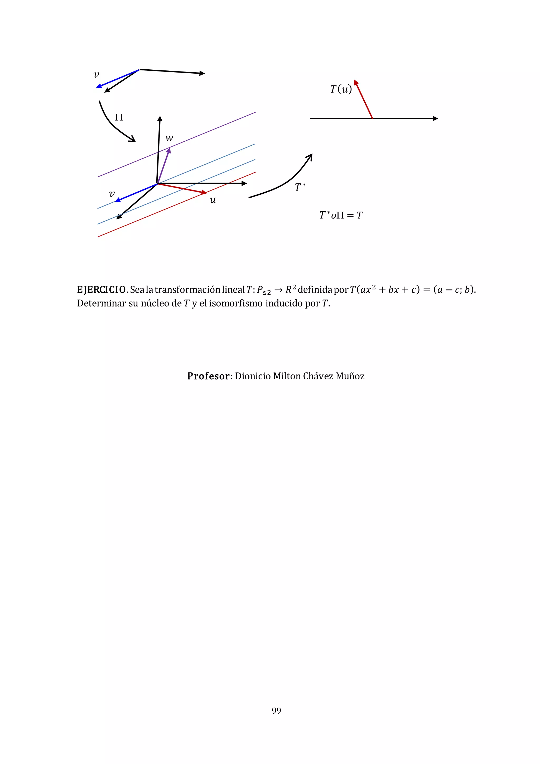
3.6 ISOMORFISMO INDUCIDO POR UNA TRANSFORMACIÓN LINEAL .
TEOREMA. Sean (𝑉;𝐾;+; ∙) y (𝑊;𝐾;+;∙)espacios vectoriales sobre el campo 𝐾, sea 𝑇:𝑉 → 𝑊
una transformación lineal y sea :𝑉 → 𝑉 𝑁(𝑇)
⁄ definida por (𝑣) = 𝑣 + 𝑁(𝑇) la proyección
canónica, entonces:
a) Existe una única transformación lineal 𝑇∗:𝑉 𝑁(𝑇)
⁄ → 𝑊 tal que 𝑇∗𝑜 = 𝑇
b) 𝑉 𝑁(𝑇)
⁄ ≅ 𝐼𝑚(𝑇): es decir que 𝑉 𝑁(𝑇)
⁄ es aproximadamente igual a 𝐼𝑚(𝑇)
En el teorema 𝑁(𝑇) el núcleo de 𝑇, y 𝑉 𝑁(𝑇)
⁄ es el espacio cociente de 𝑉 sobre 𝑁(𝑇).
Prueba.
a) Se define 𝑇∗:𝑉 𝑁(𝑇)
⁄ → 𝑊 por 𝑇∗(𝑣 + 𝑁(𝑇)) = 𝑇(𝑣)
i) Se probará que 𝑇∗ está bien definida; es decirque 𝑇∗ no depende del elemento representante
de la clase 𝑣 + 𝑁(𝑇) ∈ 𝑉 𝑁(𝑇)
⁄
Sean 𝑣1 + 𝑁(𝑇) y 𝑣2 + 𝑁(𝑇) ∈ 𝑉 𝑁(𝑇)
⁄
 Si 𝑣1 + 𝑁(𝑇) = 𝑣2 + 𝑁(𝑇)  𝑣1 = 𝑣2  𝑣1 − 𝑣2 = 0𝑉
 𝑣1 − 𝑣2 ∈ 𝑁(𝑇)  𝑇(𝑣1 − 𝑣2) = 0𝑊
 𝑇(𝑣1) − 𝑇(𝑣2) = 0𝑊  𝑇(𝑣1) = 𝑇(𝑣2) 𝑇∗(𝑣1 + 𝑁(𝑇)) = 𝑇∗(𝑣2 + 𝑁(𝑇))
𝑉 𝑁(𝑇)
⁄
𝑊
𝑉
 𝑇∗
𝑇 = 𝑇∗𝑜
𝑇

9. 95
Por lo tanto, 𝑇∗ está bien definida.
ii) 𝑇∗ es una transformación lineal.
En efecto.
𝑇∗[𝑟(𝑣1 + 𝑁(𝑇)) + 𝑡(𝑣2 + 𝑁(𝑇))]= 𝑇∗[(𝑟𝑣1 + 𝑁(𝑇)) + (𝑡𝑣2 + 𝑁(𝑇))]
= 𝑇∗[(𝑟𝑣1 + 𝑡𝑣2) + 𝑁(𝑇)] = 𝑇(𝑟𝑣1 + 𝑡𝑣2) = 𝑟𝑇(𝑣1) + 𝑡𝑇(𝑣2)
= 𝑟 𝑇∗(𝑣1 + 𝑁(𝑇)) + 𝑡 𝑇∗(𝑣2 + 𝑁(𝑇))
Por lo tanto, 𝑇∗ es una transformación lineal sobre el campo 𝐾.
iii) 𝑇∗𝑜 = 𝑇 ¡Probar!
En efecto.
(𝑇∗𝑜 )(𝑣) = 𝑇∗((𝑣)) = 𝑇∗(𝑣 + 𝑁(𝑇)) = 𝑇(𝑣)
Porlo tanto, 𝑇∗𝑜 = 𝑇
iv) La unicidad.
Supongamos que existe otra transformación lineal 𝑈∗:𝑉 𝑁(𝑇)
⁄ → 𝑊 con las mismas
propiedades que 𝑇∗.
 𝑈∗(𝑣+ 𝑁(𝑇)) = 𝑇(𝑣) = 𝑇∗(𝑣+ 𝑁(𝑇))  𝑈∗ = 𝑇∗
b) Se cumple que 𝑉 𝑁(𝑇)
⁄ ≅ 𝐼𝑚(𝑇)
Es decir, se probará que la aplicación 𝑇∗:𝑉 𝑁(𝑇)
⁄ → 𝐼𝑚(𝑇)es un isomorfismo.
i) 𝑇∗ es un monomorfismo (𝑇∗ es inyectiva).
En efecto:
𝑁(𝑇∗) = {𝑣 + 𝑁(𝑇) 𝑇∗(𝑣 + 𝑁(𝑇)) = 0𝑊
⁄ }
𝑁(𝑇∗) = {𝑣 + 𝑁(𝑇) 𝑇(𝑣) = 0𝑊
⁄ }
𝑁(𝑇∗) = {𝑣 + 𝑁(𝑇) 𝑣 ∈ 𝑁(𝑇)
⁄ }
𝑁(𝑇∗) = 𝑁(𝑇)
“𝑁(𝑇) es el cero del espacio cociente 𝑉 𝑁(𝑇)
⁄ ”
Por lo tanto, 𝑇∗ es un monomorfismo.

10. 96
ii) 𝑇∗ es un epimorfismo (𝑇∗ es sobreyectiva).
En efecto:
𝐼𝑚(𝑇∗) = {𝑇∗(𝑣+ 𝑁(𝑇)) 𝑣 ∈ 𝑉
⁄ } = {𝑇(𝑣) 𝑣 ∈ 𝑉
⁄ }= 𝐼𝑚(𝑇)
Por lo tanto, 𝑇∗ es un epimorfismo.
Finalmente, de (i) y (ii) 𝑇∗ es un isomorfismo.
EJEMPLO 1. Sea la transformación lineal 𝑇: 𝑅2 → 𝑅2 definido por 𝑇(𝑥; 𝑦) = (3𝑥 − 𝑦;𝑥 + 2𝑦).
Hallar el núcleo de 𝑇 y el isomorfismo inducido por 𝑇.
Solución.
i) Hallando el núcleo de la transformación lineal
𝑁(𝑇) = {(𝑥;𝑦) ∈ 𝑅2 𝑇(𝑥;𝑦) = (0;0)
⁄ } = {(𝑥;𝑦) ∈ 𝑅2 (3𝑥 − 𝑦;𝑥 + 2𝑦) = (0;0)
⁄ }
 (3𝑥 − 𝑦;𝑥 + 2𝑦) = (0;0)  {
3𝑥 − 𝑦 = 0
𝑥 + 2𝑦 = 0
 {
6𝑥 − 2𝑦 = 0
𝑥 + 2𝑦 = 0
 {
𝑥 = 0
𝑦 = 0
 𝑁(𝑇) = (0; 0)  𝐷𝑖𝑚(𝑁(𝑇)) = 0
ii) Hallando el espacio cociente 𝑉 𝑊
⁄ = {[𝑣] = 𝑣 + 𝑤 𝑣 ∈ 𝑉𝑤 ∈ 𝑊
⁄ }
Con los datos del ejemplo: 𝑅2 𝑁(𝑇)
⁄ = {[𝑣] = 𝑣 +  𝑣 ∈ 𝑅2 ∈ 𝑁(𝑇)
⁄ }
 𝑅2 𝑁(𝑇)
⁄ = {[𝑣] = 𝑣 + 0𝑉 𝑣 ∈ 𝑅2
⁄ }= {𝑣 𝑣 ∈ 𝑅2
⁄ }= 𝑅2.
Recordar que: 𝐷𝑖𝑚(𝑅2 {(0;0)}
⁄ ) = 𝐷𝑖𝑚(𝑅2)− 𝐷𝑖𝑚(𝑁(𝑇)) = 2 − 0 = 2
iii) Hallando el isomorfismo inducido: 𝑇∗
Aquí se tiene que  = 𝐼𝑑𝑅2
Porotro lado, 𝑇∗:𝑅2 𝑁(𝑇)
⁄ → 𝑅2  𝑇∗:𝑅2 → 𝑅2  𝑇 = 𝑇∗
La transformación lineal adjunta será: 𝑇∗[(𝑥;𝑦) + 0𝑅2 ] = (3𝑥 − 𝑦;𝑥 + 2𝑦)
𝑇∗
𝑅2 𝑅2
𝑅2 𝑁(𝑇)
⁄
𝑇
 𝑇∗
𝑅2 𝑅2
𝑅2
𝑇


11. 97
O también: 𝑇∗[(𝑥;𝑦) + 𝑁(𝑇)] = (3𝑥 − 𝑦;𝑥 + 2𝑦)
EJEMPLO 2. Sea la transformación lineal 𝑇: 𝑅2 → 𝑅2 definido por 𝑇(𝑥; 𝑦) = (0;0). Hallar el
núcleo de 𝑇 y el isomorfismo inducido por 𝑇.
Solución.
i) Hallando el núcleo de la transformación lineal
𝑁(𝑇) = {𝑣 ∈ 𝑉 𝑇(𝑣) = 0𝑊
⁄ }
𝑁(𝑇) = {(𝑥;𝑦) ∈ 𝑅2 𝑇(𝑥;𝑦) = (0;0)
⁄ }  𝑁(𝑇) = 𝑅2
ii) Hallando el espacio cociente 𝑉 𝑊
⁄ = {[𝑣] = 𝑣 + 𝑤 𝑣 ∈ 𝑉𝑤 ∈ 𝑊
⁄ }
Con los datos del ejemplo: 𝑅2 𝑅2
⁄ = {[𝑣] = 𝑣 + 𝑣 𝑣 ∈ 𝑅2 𝑣 ∈ 𝑅2
⁄ }
Usando la identidad 𝐷𝑖𝑚(𝑉 𝑊
⁄ ) = 𝐷𝑖𝑚(𝑉) − 𝐷𝑖𝑚(𝑊)
 𝐷𝑖𝑚(𝑅2 𝑅2
⁄ ) = 𝐷𝑖𝑚(𝑅2) − 𝐷𝑖𝑚(𝑅2) = 0  𝐷𝑖𝑚(𝑅2 𝑅2
⁄ ) = 0  𝑅2 𝑅2
⁄ = {(0;0)}
iii) Hallando el isomorfismo inducido: 𝑇∗
Aquí se tiene que  = (𝑥;𝑦) = (0;0)
Porotro lado, 𝑇∗:𝑅2 𝑅2
⁄ → 𝑅2  𝑇∗:{(0;0)} → 𝑅2
La transformación lineal adjunta será: 𝑇∗[(0;0) + 0𝑅2 ] = (0; 0)
O también: 𝑇∗[(0;0) + 𝑁(𝑇)] = (0; 0)
EJEMPLO 3. Sea la transformación lineal 𝑇:𝑅3 → 𝑅2 definida por 𝑇(𝑥;𝑦;𝑧) = (2𝑧 − 𝑦; 2𝑥 − 𝑧).
Determinar su núcleo de 𝑇 y el isomorfismo inducido por 𝑇.
Solución.
i) Hallando el núcleo.
𝑇∗
𝑅2 𝑅2
𝑅2 𝑅2
⁄
𝑇
 𝑇∗
𝑅2 𝑅2
{(0;0)}
𝑇


12. 98
𝑁(𝑇) = {𝑣 ∈ 𝑉 𝑇(𝑣) = 0𝑊
⁄ }
𝑁(𝑇) = {(𝑥;𝑦;𝑧) ∈ 𝑅3 𝑇(𝑥;𝑦; 𝑧) = (0; 0)
⁄ }
 (2𝑧 − 𝑦;2𝑥 − 𝑧) = (0;0)  {
2𝑧 − 𝑦 = 0
2𝑥 − 𝑧 = 0
 {
𝑦 = 2𝑧
𝑧 = −2𝑥
 {𝑦 = −4𝑥
𝑁(𝑇) = {(𝑥;𝑦;𝑧) ∈ 𝑅3 (𝑥;𝑦;𝑧) = (𝑥;−4𝑥; −2𝑥)
⁄ } , haciendo 𝑥 = 𝑡
𝑁(𝑇) = {(𝑥;𝑦;𝑧) ∈ 𝑅3 (𝑥;𝑦; 𝑧) = 𝑡(1;−4;−2), 𝑡 ∈ 𝑅
⁄ } es un subespacio (recta).
Una base del núcleo será 𝐵𝑁(𝑇) = {(1;−4; −2)} y la 𝐷𝑖𝑚(𝑁(𝑇)) = 1
ii) Hallando el espacio cociente 𝑉 𝑊
⁄ = {[𝑣] = 𝑣 + 𝑤 𝑣 ∈ 𝑉𝑤 ∈ 𝑊
⁄ }
Con los datos del ejemplo, el espacio cociente será:
𝑅3 𝑁(𝑇)
⁄ = {[𝑣] = (𝑥; 𝑦;𝑧) + 𝑡(2;−4;−2) (𝑥;𝑦;𝑧) ∈ 𝑅2 𝑡(2;−4;−2) ∈ 𝑁(𝑇)
⁄ }
Recordar que 𝐷𝑖𝑚(𝑅3 𝑁(𝑇)
⁄ ) = 𝐷𝑖𝑚(𝑅3) − 𝐷𝑖𝑚(𝑁(𝑇)) = 3 − 1 = 2
iii) Hallando el isomorfismo inducido.
Recordar: 𝑇∗:𝑉 𝑁(𝑇)
⁄ → 𝑊 por 𝑇∗(𝑣 + 𝑁(𝑇)) = 𝑇(𝑣)
Aquí se tiene que (𝑣) = 𝑣 + 𝑁(𝑇)
Porotro lado, 𝑇∗:𝑅3 𝑁(𝑇)
⁄ → 𝑅2 ; 𝑇 = 𝑇∗𝑜
 (𝑇∗𝑜)(𝑣) = 𝑇∗((𝑣)) = 𝑇∗(𝑣+ 𝑁(𝑇)) = 𝑇(𝑣)
La transformación lineal adjunta será: 𝑇∗[(𝑥;𝑦; 𝑧) + 𝑁(𝑇)] = (2𝑧 − 𝑦;2𝑥 + 𝑧)
O también: 𝑇∗[(𝑥;𝑦; 𝑧) + 𝑡(1;−4; −2)] = (2𝑧 − 𝑦; 2𝑥 + 𝑧)
Tomando algunos vectores:
Si 𝑢 = (1;5;2) ∈ 𝑅3  𝑇(1;5; 2) = (−1;4) ∈ 𝑅2
Si 𝑣 = (0; 1;3) ∈ 𝑅3  𝑇(0;1; 3) = (5;3) ∈ 𝑅2
𝑇∗
𝑅3
𝑅2
𝑅3 𝑁(𝑇)
⁄
𝑇

𝑇(𝑣)
𝑇
𝑤
𝑢

13. 99
EJERCICIO.Sealatransformaciónlineal𝑇:𝑃≤2 → 𝑅2 definidapor𝑇(𝑎𝑥2 + 𝑏𝑥 + 𝑐) = (𝑎 − 𝑐; 𝑏).
Determinar su núcleo de 𝑇 y el isomorfismo inducido por 𝑇.
Profesor: Dionicio Milton Chávez Muñoz
𝑤
𝑇(𝑢))
𝑣
𝑢
𝑇∗

𝑇∗
𝑜 = 𝑇
=T
𝑣