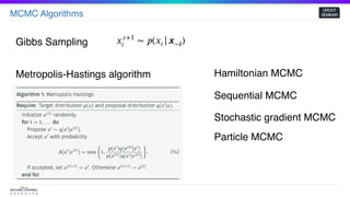
The document discusses various sampling methods used for statistical inference, focusing on latent variable models and the challenges associated with posterior sampling. It covers techniques like Monte Carlo methods, including rejection sampling and importance sampling, as well as Markov Chain Monte Carlo methods such as Gibbs sampling and Metropolis-Hastings algorithms. The emphasis throughout is on the need for approximations in Bayesian inference due to the intractability of direct computation.


![Latent Variable Model
GROOT
SEMINAR
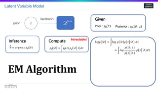
zprior
likelihood
^𝜃 = 𝑎𝑟𝑔𝑚𝑎𝑥 𝑝𝜃(𝒟)
Inference
𝑝𝜃( 𝒟) =
∫
𝑝𝜃(𝑧) 𝑝 𝜃( 𝒟 𝑧) 𝑑𝑧
Compute Intractable!
Given
Prior : 𝑝𝜃(𝑧) Posterior : 𝑝𝜃(𝒟| 𝑧)
𝒟
Data
EM Algorithm
log𝑝( 𝒟) =
∫
log 𝑝( 𝒟) 𝑝( 𝑧 𝒟) 𝑑𝑧
=
∫
𝑙𝑜𝑔
𝑝( 𝒟, 𝑧)
𝑝( 𝑧 𝒟)
𝑝( 𝑧 𝒟) 𝑑𝑧
=
∫
log𝑝( 𝒟, 𝑧) 𝑝(𝑧| 𝒟) 𝑑𝑧 −
∫
log𝑝( 𝑧 𝒟) 𝑝( 𝑧 𝒟) 𝑑𝑧
= 𝔼𝑝( 𝑧 𝒟)[log𝑝( 𝒟, 𝑧)] + 𝐻 ≥ 𝔼𝑝( 𝑧 𝒟)[log𝑝( 𝒟, 𝑧)]](https://image.slidesharecdn.com/samplingmethod-201019060419/85/Sampling-method-MCMC-15-320.jpg)
![Latent Variable Model
GROOT
SEMINAR
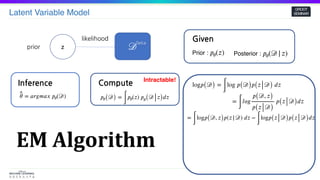
zprior
likelihood
^𝜃 = 𝑎𝑟𝑔𝑚𝑎𝑥 𝑝𝜃(𝒟)
Inference
𝑝𝜃( 𝒟) =
∫
𝑝𝜃(𝑧) 𝑝 𝜃( 𝒟 𝑧) 𝑑𝑧
Compute Intractable!
Given
Prior : 𝑝𝜃(𝑧) Posterior : 𝑝𝜃(𝒟| 𝑧)
𝒟
Data
EM Algorithm
log𝑝( 𝒟) =
∫
log 𝑝( 𝒟) 𝑝( 𝑧 𝒟) 𝑑𝑧
=
∫
𝑙𝑜𝑔
𝑝( 𝒟, 𝑧)
𝑝( 𝑧 𝒟)
𝑝( 𝑧 𝒟) 𝑑𝑧
=
∫
log𝑝( 𝒟, 𝑧) 𝑝(𝑧| 𝒟) 𝑑𝑧 −
∫
log𝑝( 𝑧 𝒟) 𝑝( 𝑧 𝒟) 𝑑𝑧
= 𝔼𝑝( 𝑧 𝒟)[log𝑝( 𝒟, 𝑧)] + 𝐻 ≥ 𝔼𝑝( 𝑧 𝒟)[log𝑝( 𝒟, 𝑧)]
E-Step](https://image.slidesharecdn.com/samplingmethod-201019060419/85/Sampling-method-MCMC-16-320.jpg)
![Latent Variable Model
GROOT
SEMINAR
zprior
likelihood
^𝜃 = 𝑎𝑟𝑔𝑚𝑎𝑥 𝑝𝜃(𝒟)
Inference
𝑝𝜃( 𝒟) =
∫
𝑝𝜃(𝑧) 𝑝 𝜃( 𝒟 𝑧) 𝑑𝑧
Compute Intractable!
Given
Prior : 𝑝𝜃(𝑧) Posterior : 𝑝𝜃(𝒟| 𝑧)
𝒟
Data
EM Algorithm
log𝑝( 𝒟) =
∫
log 𝑝( 𝒟) 𝑝( 𝑧 𝒟) 𝑑𝑧
=
∫
𝑙𝑜𝑔
𝑝( 𝒟, 𝑧)
𝑝( 𝑧 𝒟)
𝑝( 𝑧 𝒟) 𝑑𝑧
=
∫
log𝑝( 𝒟, 𝑧) 𝑝(𝑧| 𝒟) 𝑑𝑧 −
∫
log𝑝( 𝑧 𝒟) 𝑝( 𝑧 𝒟) 𝑑𝑧
= 𝔼𝑝( 𝑧 𝒟)[log𝑝( 𝒟, 𝑧)] + 𝐻 ≥ 𝔼𝑝( 𝑧 𝒟)[log𝑝( 𝒟, 𝑧)]
E-Step
𝑝( 𝑧 𝒟) =
𝑝( 𝒟, 𝑧)
𝑝(𝒟)](https://image.slidesharecdn.com/samplingmethod-201019060419/85/Sampling-method-MCMC-17-320.jpg)
![Latent Variable Model
GROOT
SEMINAR
zprior
likelihood
^𝜃 = 𝑎𝑟𝑔𝑚𝑎𝑥 𝑝𝜃(𝒟)
Inference
𝑝𝜃( 𝒟) =
∫
𝑝𝜃(𝑧) 𝑝 𝜃( 𝒟 𝑧) 𝑑𝑧
Compute Intractable!
Given
Prior : 𝑝𝜃(𝑧) Posterior : 𝑝𝜃(𝒟| 𝑧)
𝒟
Data
EM Algorithm
log𝑝( 𝒟) =
∫
log 𝑝( 𝒟) 𝑝( 𝑧 𝒟) 𝑑𝑧
=
∫
𝑙𝑜𝑔
𝑝( 𝒟, 𝑧)
𝑝( 𝑧 𝒟)
𝑝( 𝑧 𝒟) 𝑑𝑧
=
∫
log𝑝( 𝒟, 𝑧) 𝑝(𝑧| 𝒟) 𝑑𝑧 −
∫
log𝑝( 𝑧 𝒟) 𝑝( 𝑧 𝒟) 𝑑𝑧
= 𝔼𝑝( 𝑧 𝒟)[log𝑝( 𝒟, 𝑧)] + 𝐻 ≥ 𝔼𝑝( 𝑧 𝒟)[log𝑝( 𝒟, 𝑧)]
E-Step
𝑝( 𝑧 𝒟) =
𝑝( 𝒟, 𝑧)
𝑝(𝒟)
Intractable!](https://image.slidesharecdn.com/samplingmethod-201019060419/85/Sampling-method-MCMC-18-320.jpg)
![Latent Variable Model
GROOT
SEMINAR
zprior
likelihood
^𝜃 = 𝑎𝑟𝑔𝑚𝑎𝑥 𝑝𝜃(𝒟)
Inference
𝑝𝜃( 𝒟) =
∫
𝑝𝜃(𝑧) 𝑝 𝜃( 𝒟 𝑧) 𝑑𝑧
Compute Intractable!
Given
Prior : 𝑝𝜃(𝑧) Posterior : 𝑝𝜃(𝒟| 𝑧)
Posterior inference
𝔼[ 𝑧 𝒟] 𝔼[ 𝑓(𝑧) 𝒟]
𝒟
Data](https://image.slidesharecdn.com/samplingmethod-201019060419/85/Sampling-method-MCMC-19-320.jpg)
![Latent Variable Model
GROOT
SEMINAR
zprior
likelihood
^𝜃 = 𝑎𝑟𝑔𝑚𝑎𝑥 𝑝𝜃(𝒟)
Inference
𝑝𝜃( 𝒟) =
∫
𝑝𝜃(𝑧) 𝑝 𝜃( 𝒟 𝑧) 𝑑𝑧
Compute Intractable!
Given
Prior : 𝑝𝜃(𝑧) Posterior : 𝑝𝜃(𝒟| 𝑧)
Posterior inference
𝔼[ 𝑧 𝒟] 𝔼[ 𝑓(𝑧) 𝒟]
𝒟
Data](https://image.slidesharecdn.com/samplingmethod-201019060419/85/Sampling-method-MCMC-20-320.jpg)
![Latent Variable Model
GROOT
SEMINAR
zprior
likelihood
^𝜃 = 𝑎𝑟𝑔𝑚𝑎𝑥 𝑝𝜃(𝒟)
Inference
𝑝𝜃( 𝒟) =
∫
𝑝𝜃(𝑧) 𝑝 𝜃( 𝒟 𝑧) 𝑑𝑧
Compute Intractable!
Given
Prior : 𝑝𝜃(𝑧) Posterior : 𝑝𝜃(𝒟| 𝑧)
Posterior inference
𝔼[ 𝑧 𝒟] 𝔼[ 𝑓(𝑧) 𝒟]
𝒟
Data
“Bayesian inference is all about posterior inference”](https://image.slidesharecdn.com/samplingmethod-201019060419/85/Sampling-method-MCMC-21-320.jpg)
![Latent Variable Model
GROOT
SEMINAR
zprior
likelihood
^𝜃 = 𝑎𝑟𝑔𝑚𝑎𝑥 𝑝𝜃(𝒟)
Inference
𝑝𝜃( 𝒟) =
∫
𝑝𝜃(𝑧) 𝑝 𝜃( 𝒟 𝑧) 𝑑𝑧
Compute Intractable!
Given
Prior : 𝑝𝜃(𝑧) Posterior : 𝑝𝜃(𝒟| 𝑧)
Posterior inference
𝔼[ 𝑧 𝒟] 𝔼[ 𝑓(𝑧) 𝒟]
𝒟
Data
Direct computing is impossible
“Bayesian inference is all about posterior inference”](https://image.slidesharecdn.com/samplingmethod-201019060419/85/Sampling-method-MCMC-22-320.jpg)
![Latent Variable Model
GROOT
SEMINAR
zprior
likelihood
^𝜃 = 𝑎𝑟𝑔𝑚𝑎𝑥 𝑝𝜃(𝒟)
Inference
𝑝𝜃( 𝒟) =
∫
𝑝𝜃(𝑧) 𝑝 𝜃( 𝒟 𝑧) 𝑑𝑧
Compute Intractable!
Given
Prior : 𝑝𝜃(𝑧) Posterior : 𝑝𝜃(𝒟| 𝑧)
Posterior inference
𝔼[ 𝑧 𝒟] 𝔼[ 𝑓(𝑧) 𝒟]
𝒟
Data
Direct computing is impossible
Approximation! But…how?
“Bayesian inference is all about posterior inference”](https://image.slidesharecdn.com/samplingmethod-201019060419/85/Sampling-method-MCMC-23-320.jpg)
![Latent Variable Model
GROOT
SEMINAR
zprior
likelihood
^𝜃 = 𝑎𝑟𝑔𝑚𝑎𝑥 𝑝𝜃(𝒟)
Inference
𝑝𝜃( 𝒟) =
∫
𝑝𝜃(𝑧) 𝑝 𝜃( 𝒟 𝑧) 𝑑𝑧
Compute Intractable!
Given
Prior : 𝑝𝜃(𝑧) Posterior : 𝑝𝜃(𝒟| 𝑧)
Posterior inference
𝔼[ 𝑧 𝒟] 𝔼[ 𝑓(𝑧) 𝒟]
𝒟
Data
Direct computing is impossible
Approximation! But…how?
“Bayesian inference is all about posterior inference”
Let target distribution denoted by 𝑝(𝑥)](https://image.slidesharecdn.com/samplingmethod-201019060419/85/Sampling-method-MCMC-24-320.jpg)


![Monte Carlo Method
GROOT
SEMINAR
The Law of Large Numbers
𝑋1 + 𝑋2 + ⋯ + 𝑋𝑛
𝑛
→ 𝔼[𝑋𝑖]𝑋1, 𝑋2, …, 𝑋𝑛 : 𝑖 . 𝑖 . 𝑑](https://image.slidesharecdn.com/samplingmethod-201019060419/85/Sampling-method-MCMC-34-320.jpg)
![Monte Carlo Method
GROOT
SEMINAR
The Law of Large Numbers
𝑋1 + 𝑋2 + ⋯ + 𝑋𝑛
𝑛
→ 𝔼[𝑋𝑖]𝑋1, 𝑋2, …, 𝑋𝑛 : 𝑖 . 𝑖 . 𝑑
But…](https://image.slidesharecdn.com/samplingmethod-201019060419/85/Sampling-method-MCMC-35-320.jpg)
![Monte Carlo Method
GROOT
SEMINAR
The Law of Large Numbers
𝑋1 + 𝑋2 + ⋯ + 𝑋𝑛
𝑛
→ 𝔼[𝑋𝑖]𝑋1, 𝑋2, …, 𝑋𝑛 : 𝑖 . 𝑖 . 𝑑
But… Yes, How do we sample from ?𝑝(𝑥)](https://image.slidesharecdn.com/samplingmethod-201019060419/85/Sampling-method-MCMC-36-320.jpg)
![Monte Carlo Method
GROOT
SEMINAR
The Law of Large Numbers
𝑋1 + 𝑋2 + ⋯ + 𝑋𝑛
𝑛
→ 𝔼[𝑋𝑖]𝑋1, 𝑋2, …, 𝑋𝑛 : 𝑖 . 𝑖 . 𝑑
But… Yes, How do we sample from ?𝑝(𝑥)
Rejection Sampling](https://image.slidesharecdn.com/samplingmethod-201019060419/85/Sampling-method-MCMC-37-320.jpg)
![Monte Carlo Method
GROOT
SEMINAR
The Law of Large Numbers
𝑋1 + 𝑋2 + ⋯ + 𝑋𝑛
𝑛
→ 𝔼[𝑋𝑖]𝑋1, 𝑋2, …, 𝑋𝑛 : 𝑖 . 𝑖 . 𝑑
But… Yes, How do we sample from ?𝑝(𝑥)
: proposal distribution𝑞(𝑥)
Rejection Sampling
Easy to compute, easy to sample](https://image.slidesharecdn.com/samplingmethod-201019060419/85/Sampling-method-MCMC-38-320.jpg)
![Monte Carlo Method
GROOT
SEMINAR
The Law of Large Numbers
𝑋1 + 𝑋2 + ⋯ + 𝑋𝑛
𝑛
→ 𝔼[𝑋𝑖]𝑋1, 𝑋2, …, 𝑋𝑛 : 𝑖 . 𝑖 . 𝑑
But… Yes, How do we sample from ?𝑝(𝑥)
: proposal distribution𝑞(𝑥)
Rejection Sampling
Easy to compute, easy to sample
𝑀𝑞(𝑥) ≥ ~𝑝(𝑥)
If , we reject the sample, otherwise we accept it𝑢 >
~𝑝(𝑥)
𝑀𝑞(𝑥)](https://image.slidesharecdn.com/samplingmethod-201019060419/85/Sampling-method-MCMC-39-320.jpg)
![Monte Carlo Method
GROOT
SEMINAR
The Law of Large Numbers
𝑋1 + 𝑋2 + ⋯ + 𝑋𝑛
𝑛
→ 𝔼[𝑋𝑖]𝑋1, 𝑋2, …, 𝑋𝑛 : 𝑖 . 𝑖 . 𝑑
But… Yes, How do we sample from ?𝑝(𝑥)
: proposal distribution𝑞(𝑥)
Rejection Sampling
Easy to compute, easy to sample
𝑀𝑞(𝑥) ≥ ~𝑝(𝑥)
If , we reject the sample, otherwise we accept it𝑢 >
~𝑝(𝑥)
𝑀𝑞(𝑥)](https://image.slidesharecdn.com/samplingmethod-201019060419/85/Sampling-method-MCMC-40-320.jpg)

![Monte Carlo Method
GROOT
SEMINAR
𝜇 = 𝔼𝑝(𝑥)[ 𝑓(𝑥)] =
∫
𝑓(𝑥)
~𝑝(𝑥)
𝑍
𝑑𝑥 =
1
𝑍 ∫
𝑓(𝑥)
~𝑝(𝑥)
𝑞(𝑥)
𝑞(𝑥)𝑑𝑥
Importance Samping](https://image.slidesharecdn.com/samplingmethod-201019060419/85/Sampling-method-MCMC-42-320.jpg)
![Monte Carlo Method
GROOT
SEMINAR
𝜇 = 𝔼𝑝(𝑥)[ 𝑓(𝑥)] =
∫
𝑓(𝑥)
~𝑝(𝑥)
𝑍
𝑑𝑥 =
1
𝑍 ∫
𝑓(𝑥)
~𝑝(𝑥)
𝑞(𝑥)
𝑞(𝑥)𝑑𝑥
Importance Samping
𝔼𝑝(𝑥)[ 𝑓(𝑥)] ≈
1
𝑛𝑍 ∑
𝑓( 𝑥𝑖)
~𝑝( 𝑥𝑖)
𝑞( 𝑥𝑖)
=
1
𝑛𝑍 ∑
𝑤( 𝑥𝑖) 𝑓(𝑥𝑖)
𝑍 =
∫
~𝑝(𝑥)𝑑𝑥 =
∫
~𝑝(𝑥)
𝑞(𝑥)
𝑞(𝑥)𝑑𝑥 ≈
1
𝑛 ∑
𝑤(𝑥𝑖)
𝔼𝑝(𝑥)[ 𝑓(𝑥)] ≈
∑
~𝑤( 𝑥𝑖) 𝑓(𝑥𝑖)](https://image.slidesharecdn.com/samplingmethod-201019060419/85/Sampling-method-MCMC-43-320.jpg)
![Monte Carlo Method
GROOT
SEMINAR
𝜇 = 𝔼𝑝(𝑥)[ 𝑓(𝑥)] =
∫
𝑓(𝑥)
~𝑝(𝑥)
𝑍
𝑑𝑥 =
1
𝑍 ∫
𝑓(𝑥)
~𝑝(𝑥)
𝑞(𝑥)
𝑞(𝑥)𝑑𝑥
Importance Samping
𝔼𝑝(𝑥)[ 𝑓(𝑥)] ≈
1
𝑛𝑍 ∑
𝑓( 𝑥𝑖)
~𝑝( 𝑥𝑖)
𝑞( 𝑥𝑖)
=
1
𝑛𝑍 ∑
𝑤( 𝑥𝑖) 𝑓(𝑥𝑖)
𝑍 =
∫
~𝑝(𝑥)𝑑𝑥 =
∫
~𝑝(𝑥)
𝑞(𝑥)
𝑞(𝑥)𝑑𝑥 ≈
1
𝑛 ∑
𝑤(𝑥𝑖)
𝔼𝑝(𝑥)[ 𝑓(𝑥)] ≈
∑
~𝑤( 𝑥𝑖) 𝑓(𝑥𝑖)
i.i.d sampling is very vulnerable in high-dimensional spaces](https://image.slidesharecdn.com/samplingmethod-201019060419/85/Sampling-method-MCMC-44-320.jpg)

![Basic idea of MCMC
GROOT
SEMINAR
Markov Chain :
𝑝( 𝑥(𝑡+1)
𝑥(1), 𝑥(2)
, …, 𝑥(𝑡)
) = 𝑝( 𝑥(𝑡+1)
𝑥(𝑡)
)
is a sequence of random variables. It forms a Markov chain if𝑥(1)
, 𝑥(2)
, …
A Markov chain can be specified by
1. Initial distribution
2. Transition probability
𝑝1(𝑥) = 𝑝( 𝑥(1)
)
𝑇 𝑘(𝑥′, 𝑥) = 𝑝( 𝑥(𝑡+1)
= 𝑥′ 𝑥(𝑡)
= 𝑥)
Ergodicity
, regardless of the initial distributionlim
𝑛→∞
𝑇 𝑛
𝑝1 = 𝜋 𝑝1
1. Build a Markov chain having
as an invariant distribution
2. Sample from the chain
3. Compute
𝑝(𝑥)
( 𝑥(𝑡)
)𝑡≥1
𝔼𝑝(𝑥)[ 𝑓(𝑥)] ≈ 𝔼 𝑇 𝑛 𝑝1(𝑥)[ 𝑓(𝑥)]
≈
1
𝑛 ∑
𝑓( 𝑥(𝑡)
)](https://image.slidesharecdn.com/samplingmethod-201019060419/85/Sampling-method-MCMC-46-320.jpg)