This document discusses differential equations. It defines differential equations as equations relating an unknown function and one or more of its derivatives. It describes the order and degree of differential equations. Several examples of first order differential equations are given and solved using techniques like direct integration, variable separation, and solving homogeneous equations. The key steps for solving first order differential equations are outlined.
The document provides an introduction to partial differential equations (PDEs). Some key points:
- PDEs involve functions of two or more independent variables, and arise in physics/engineering problems.
- PDEs contain partial derivatives with respect to two or more independent variables. Examples of common PDEs are given, including the Laplace, wave, and heat equations.
- The order of a PDE is defined as the order of the highest derivative. Methods for solving PDEs through direct integration and using Lagrange's method are briefly outlined.
This document discusses differential equations and includes the following key points:
1. It defines differential equations and provides examples of ordinary and partial differential equations of varying orders.
2. It classifies differential equations as ordinary or partial, linear or non-linear, and of first or higher order. Examples are given of each type.
3. Applications of differential equations are listed, including modeling projectile motion, electric circuits, heat transfer, vibrations, population growth, and chemical reactions.
4. Methods of solving differential equations including finding general and particular solutions are explained. Initial value and boundary value problems are also defined.
First order linear differential equationNofal Umair
1. A differential equation relates an unknown function and its derivatives, and can be ordinary (involving one variable) or partial (involving partial derivatives).
2. Linear differential equations have dependent variables and derivatives that are of degree one, and coefficients that do not depend on the dependent variable.
3. Common methods for solving first-order linear differential equations include separation of variables, homogeneous equations, and exact equations.
This document provides an introduction to differential equations. It defines a differential equation as an equation containing an unknown function and its derivatives. Ordinary differential equations are presented, along with definitions of the order and degree of a differential equation. Methods for solving differential equations are introduced, including Taylor series methods, Euler's method, and error analysis. Examples are provided to demonstrate applying these methods.
This document provides two examples of using double and triple integrals to calculate the moment of inertia and volume of solids. The first example calculates the moment of inertia of a solid inside a cylinder using cylindrical coordinates. The second example finds the volume of a solid inside a sphere and outside a cone using spherical coordinates. It converts the equations to spherical coordinates and sets up the integral to evaluate the volume.
This document provides an introduction to differential equations. It defines differential equations as equations containing an unknown function and its derivatives. It discusses ordinary differential equations which contain one independent variable and partial differential equations which can contain multiple independent variables. The order of a differential equation refers to the order of the highest derivative term. The degree of a differential equation is the power of the highest order derivative term. Linear differential equations have dependent variables and derivatives that are of degree one and have coefficients that do not depend on the dependent variable. Several examples of different types of differential equations are provided.
1. The differentiation formulas for the trigonometric functions sin(u), cos(u), tan(u), cot(u), sec(u), and csc(u) are presented in terms of their derivatives du/dx.
2. The derivatives are obtained by applying the basic differentiation formulas for sin(u) and cos(u) along with the quotient, product, and chain rules.
3. Formulas are also provided for deriving the derivatives of inverse trigonometric functions like arcsin, arccos, arctan, etc.
- A differential equation involves an independent variable, dependent variable, and derivatives of the dependent variable with respect to the independent variable.
- The order of a differential equation is the order of the highest derivative, and the degree is the exponent of the highest order derivative.
- Linear differential equations involve the dependent variable and its derivatives only to the first power. Non-linear equations do not meet this criterion.
- The general solution of a differential equation contains as many arbitrary constants as the order of the equation. A particular solution results from assigning values to the arbitrary constants.
- Differential equations can be solved through methods like variable separation, inspection of reducible forms, and finding homogeneous or linear representations.
The z-transform provides a method to analyze discrete-time signals and systems using complex variable theory. It is defined as the summation of a sequence multiplied by z to the power of the time index from negative infinity to positive infinity. The region of convergence consists of values of z where this summation converges. It is determined by the locations of the zeros and poles of the z-transform function. Examples show how different sequences lead to different regions of convergence bounded by these zeros and poles.
Fourier series can be used to represent periodic and discontinuous functions. The document discusses:
1. The Fourier series expansion of a sawtooth wave, showing how additional terms improve the accuracy of the representation.
2. How Fourier series are well-suited to represent periodic functions over intervals like [0,2π] since the basis functions are also periodic.
3. An example of using Fourier series to analyze a square wave, finding the coefficients for its expansion in terms of sines and cosines.
This document discusses differentiable and analytic functions of a complex variable z. It defines the derivative of a complex function f(z) and shows that for f(z) to be differentiable, the Cauchy-Riemann equations relating the partial derivatives of the real and imaginary parts must be satisfied. Examples are provided to illustrate calculating derivatives and determining differentiability. The document also covers power series representations of functions, elementary functions like exponential and logarithmic functions, and the concepts of branch points and cuts for multi-valued complex functions.
The document discusses joint and marginal probability distributions of random variables. It provides examples of defining joint probability functions p(x,y) for two random variables X and Y based on a card hand experiment and dice rolling experiment. It also discusses calculating marginal probabilities by summing the joint probabilities over all values of one variable. Conditional probabilities are defined as the probability of one variable given a particular value of the other.
The document discusses encoders, decoders, multiplexers (MUX), and how they can be used to implement digital logic functions. It provides examples of using 4-to-1, 8-to-1 and 10-to-1 MUX to implement functions. It also gives examples of 4-to-2, 8-to-3 and 10-to-4 encoders. Decoder examples include a 2-to-4 and 3-to-8 binary decoder. The document explains how decoders can be used as logic building blocks to realize Boolean functions. It poses questions to be answered using terms like MUX, DEMUX, encoder, decoder.
Flipflops and Excitation tables of flipflopsstudent
This document discusses latches and flip-flops. It explains that gates perform logic operations while flip-flops can store binary values. There are two types of sequential logic circuits: combinational using gates and sequential using flip-flops like the SR, D, JK, and T flip-flops. Flip-flops change state based on clock pulses in synchronous circuits or independent of clocks in asynchronous circuits.
This document discusses signals and systems. It defines signals as physical quantities that vary with respect to time, space, or another independent variable. Signals can be classified as discrete time or continuous time. It also defines unit impulse and unit step functions for discrete and continuous time. Periodic and aperiodic signals are discussed. The Fourier series and Fourier transform are introduced as ways to represent signals in the frequency domain. The Laplace transform, which generalizes the Fourier transform, is also mentioned. Key properties of linear time-invariant systems like superposition, time-invariance, and convolution are covered. Finally, sampling theory and the z-transform, which is analogous to the Laplace transform for discrete-time systems, are summarized at a high level
This document provides an introduction to ordinary differential equations (ODEs). It defines ODEs as differential equations containing functions of one independent variable and its derivatives. The document discusses some key concepts related to ODEs including order, degree, and different types of ODEs such as variable separable, homogeneous, exact, linear, and Bernoulli's equations. Examples of each type of ODE are provided along with the general methods for solving each type.
SERIES SOLUTION OF ORDINARY DIFFERENTIALL EQUATIONKavin Raval
This document discusses methods for solving ordinary differential equations (ODEs) using power series solutions and the Frobenius method. The power series method assumes solutions of the form of a power series centered at an ordinary point. The Frobenius method extends this to regular singular points by assuming solutions of the form of a power series multiplied by (x-x0)^r, where r is determined from the indicial equation. The document outlines the steps for both methods, which involve substituting the assumed series into the ODE and equating coefficients of like powers of (x-x0).
- The document discusses Fourier series and integrals.
- Fourier series decomposes a periodic function into a sum of sines and cosines. It is useful for representing periodic and discontinuous functions.
- There are three types of Fourier integrals: the general Fourier integral, Fourier cosine integral, and Fourier sine integral. These are used to represent functions over infinite intervals.
The document defines and provides examples of differential equations. The key points are:
- A differential equation is an equation involving one or more independent variables, one dependent variable, and the derivatives of the dependent variable.
- Differential equations can be ordinary (contain one independent variable) or partial (contain two or more independent variables).
- The order of a differential equation is the order of the highest derivative. The degree refers to the highest power of the highest derivative when expressed as a polynomial.
- The general solution of a differential equation contains as many arbitrary constants as the order of the equation. A particular solution assigns specific values to the constants.
This presentation gives the basic idea about the methods of solving ODEs
The methods like variation of parameters, undetermined coefficient method, 1/f(D) method, Particular integral and complimentary functions of an ODE
1) The document presents information on ordinary differential equations including definitions, types, order, degree, and solution methods.
2) Differential equations can be written in derivative, differential, and differential operator forms. Common solution methods covered are variable separable, homogeneous, linear, and exact differential equations.
3) Applications of differential equations include physics, astronomy, meteorology, chemistry, biology, ecology, and economics for modeling various real-world systems.
Its states Periodic function, Fourier series for disontinous function, Fourier series, Intervals, Odd and even functions, Half range fourier series etc. Mostly used as active learning assignment in Degree 3rd sem students.
The document summarizes the complex form of Fourier series. It states that after substituting sine and cosine terms into the Fourier series formula, the complex form involves a summation of terms with coefficients multiplied by exponential terms with integer multiples of i and x. It provides the formulas for calculating the coefficients c0, c1, c2, etc. and gives an example function defined over an interval to demonstrate the complex form.
This document discusses a course on electromagnetic theory taught by Arpan Deyasi. It covers topics related to vector differentiation, including the vector differential operator in Cartesian, cylindrical and spherical coordinates. It also covers differentiation of scalar functions, including calculating gradients, directional derivatives and finding normals to surfaces. Finally, it discusses differentiation of vector functions, specifically divergence, which represents the volume density of the net outward flux from a vector field.
This document provides an introduction and overview of differential equations including:
- It defines differential equations as equations that relate an unknown function to its derivatives.
- It classifies differential equations as ordinary or partial, and discusses homogeneous differential equations which can be solved using separation of variables.
- It provides examples of linear differential equations and discusses their applications in areas like software development, modeling natural phenomena, and theories.
- In conclusion, it states that differential equations are essential for both engineers and non-engineers as they underpin many software programs and describe the natural world.
Introduction to operational Amplifier. For A2 level physics (CIE). Discusses characteristics of op amp, inverting and non inverting amplifier, and voltage follower, and transfer characetristics, virtual earth , etc
This document defines and provides examples of linear differential equations. It discusses:
1) Linear differential equations can be written in the form P(x)y'=Q(x) or P(y)x'=Q(y), where multiplying both sides by an integrating factor μ results in a total derivative.
2) First order linear differential equations of the form P(x)y'=Q(x) have an integrating factor of e∫P(x)dx. The general solution is y(IF)=C.
3) Bernoulli's equation is a differential equation of the form P(x)y'+Q(x)y^n=R(x), where the general solution depends
The document discusses higher order differential equations. It defines nth order differential equations and describes their general forms. For homogeneous equations, the general solution method involves making an operator form, constructing an auxiliary equation, solving for roots, and finding the complementary solution. For non-homogeneous equations, the method of undetermined coefficients is used to find a particular solution and the general solution is the sum of the complementary and particular solutions. Examples are provided to illustrate the solution methods.
The document discusses partial differential equations and their solutions. It can be summarized as:
1) A partial differential equation involves a function of two or more variables and some of its partial derivatives, with one dependent variable and one or more independent variables. Standard notation is presented for partial derivatives.
2) Partial differential equations can be formed by eliminating arbitrary constants or arbitrary functions from an equation relating the dependent and independent variables. Examples of each method are provided.
3) Solutions to partial differential equations can be complete, containing the maximum number of arbitrary constants allowed, particular where the constants are given specific values, or singular where no constants are present. Methods for determining the general solution are described.
This document discusses differential equations. It begins by explaining that differential equations are used to model many physical phenomena in areas like economics, engineering, and more. It then provides examples of ordinary and partial differential equations. The rest of the document defines key terms related to differential equations like order, degree, families of curves, and how to derive the differential equation of a family of curves by eliminating parameters. Several examples are provided to illustrate these concepts.
Here are the key steps to solve this separable differential equation:
1) Separate the variables: dy/dx = (1-y^2)
2) Integrate both sides: ∫ dy/(1-y^2) = ∫ dx
3) Evaluate the integrals: arctan(y) = x + C
4) Take the inverse tangent of both sides: y = tan(x + C)
This is the general solution.
1.4
Transformations
We can transform a differential equation into a separable one using the following techniques:
So the general solution is:
y = tan(x + C)
1. Change of variables:
This document discusses numerical methods for solving differential equations. It provides examples of linear, exponential, and logistic differential equation models. It also discusses predator-prey models defined by a system of two coupled differential equations that cannot be solved analytically. The Fitzhugh-Nagumo model is presented as another example of a system of differential equations that can be analyzed using phase plane analysis and numerical methods.
The document discusses differential equations and their use in mathematical modeling of physical phenomena. It provides examples of differential equations describing free fall with air resistance, mouse and owl populations, and water pollution. Direction fields are used to graphically analyze solution behaviors and equilibrium solutions for various differential equations.
This document outlines the contents and references for the unit on linear differential equations of second and higher order. The unit covers topics such as complementary functions, particular integrals, Cauchy's linear equations, Legendre's linear equations, and the method of variation of parameters. It provides 18 slides covering these topics, including examples of solving differential equations using each method. The unit is part of a course on engineering mathematics for first year students.
Differential Equations Lecture: Non-Homogeneous Linear Differential Equationsbullardcr
This document discusses the method of undetermined coefficients for solving nonhomogeneous second-order linear differential equations. It explains that the solution to a nonhomogeneous equation is the sum of the solution to the corresponding homogeneous equation and a particular solution to account for the nonhomogeneous term. It also outlines the steps to use the method of undetermined coefficients, which involves guessing a form for the particular solution based on the type of nonhomogeneous term and solving for the coefficients.
Delay-Differential Equations. Tools for Epidemics ModellingIgnasi Gros
The document discusses delay-differential equations which are used to model epidemics. It provides examples of delay-differential equations and their solutions. Solutions to delay-differential equations involve an infinite number of terms due to the dependence on past values. The behavior of solutions depends on the characteristics of the individual terms, with some terms potentially growing and others decaying over time. Delay-differential equations are used to model more complex epidemic models that account for factors like incubation periods.
Differential equation & laplace transformation with matlabRavi Jindal
This document discusses using MATLAB to solve differential equations through Laplace transformations. It introduces key terms like the Laplace operator and generating function. It then demonstrates how to use MATLAB commands like "laplace" and "ilaplace" to calculate the Laplace transform of a function and take the inverse Laplace transform. Examples are provided, such as finding the Laplace transform of the function f(t)=-1.25+3.5t*exp(-2t)+1.25*exp(-2t).
Numerical Method Analysis: Algebraic and Transcendental Equations (Non-Linear)Minhas Kamal
Numerical Method Analysis- Solution of Algebraic and Transcendental Equations (Non-Linear Equation). Algorithms- Bisection Method, False Position Method, Newton-Raphson Method, Secant Method, Successive Approximation Method.
Visit here for getting code implementation- https://github.com/MinhasKamal/AlgorithmImplementations/blob/master/numericalMethods/equationSolving/NonLinearEquationSolvingProcess.c
Created in 2nd year of Bachelor of Science in Software Engineering (BSSE) course at Institute of Information Technology, University of Dhaka (IIT, DU).
An Introduction to Real Analysis & Differential EquationsDhananjay Goel
The First 15 Pages of the first year course MAL 111, titled, An Introduction to Real Analysis & Differential Equations. For more Visit www.study-india.co.in or www.iitnotes.com
Application of differential equation in real lifeTanjil Hasan
Differential equations are used in many areas of real life including creating software, games, artificial intelligence, modeling natural phenomena, and providing theoretical explanations. Some examples given are using differential equations to model character velocity in games, understand computer hardware, solve constraint logic programs, describe physical laws, and model chemical reaction rates. Differential equations are an essential mathematical tool for describing how our world works.
Ch 05 MATLAB Applications in Chemical Engineering_陳奇中教授教學投影片Chyi-Tsong Chen
The slides of Chapter 5 of the book entitled "MATLAB Applications in Chemical Engineering": Numerical Solution of Partial Differential Equations. Author: Prof. Chyi-Tsong Chen (陳奇中教授); Center for General Education, National Quemoy University; Kinmen, Taiwan; E-mail: chyitsongchen@gmail.com.
Ebook purchase: https://play.google.com/store/books/details/MATLAB_Applications_in_Chemical_Engineering?id=kpxwEAAAQBAJ&hl=en_US&gl=US
The document presents information about differential equations including:
- A definition of a differential equation as an equation containing the derivative of one or more variables.
- Classification of differential equations by type (ordinary vs. partial), order, and linearity.
- Methods for solving different types of differential equations such as variable separable form, homogeneous equations, exact equations, and linear equations.
- An example problem demonstrating how to use the cooling rate formula to calculate the time of death based on measured body temperatures.
The document defines probability as the ratio of desired outcomes to total outcomes. It provides examples of calculating probabilities of outcomes from rolling a die or flipping a coin. It explains that probabilities of all outcomes must sum to 1. It also discusses calculating probabilities of multiple events using "and" or "or", and defines experimental probability as the ratio of outcomes to trials from an experiment.
4 the not so trivial pursuit of full alignmentmikegggg
This document discusses the importance of organizational alignment and the dangers of misalignment. It argues that misalignments, if left unaddressed, can grow and seriously undermine an organization's performance, efficiency and ability to adapt. The document identifies some common sources of misalignment, such as misaligned expectations, capabilities, responsibilities and goals. It stresses that leaders have a responsibility to identify and resolve misalignments in order to build high-performing organizations.
This document is a transcript of delinquent land taxes available for sale in Colbert County, Alabama. It lists the names of taxpayers who owe property taxes, the amounts owed for state, county, municipal taxes, fees, interest, administrative costs and total owed. It also provides parcel numbers, property descriptions and notes such as deeds, dwellings or irregular parcels. The transcript contains over 30 listings of delinquent taxpayers and properties.
The document discusses separable differential equations, which can be expressed as the product of a function of x and a function of y. An example separable differential equation is provided, along with steps to solve it by separating the variables. The solution yields an implicit relationship between y and x. A second example problem is presented to illustrate solving a separable differential equation with an initial condition.
12 x1 t07 02 v and a in terms of x (2012)Nigel Simmons
1) The document discusses relating acceleration to velocity and position for particles moving in one dimension.
2) It derives the formula for acceleration as the second derivative of position with respect to time, equal to the first derivative of velocity with respect to position.
3) It provides two examples:
- Example 1 finds the velocity of a particle in terms of its position by solving the differential equation for acceleration.
- Example 2 finds the position of a particle in terms of time by solving the differential equation and using initial conditions.
This document provides information on differentiation including:
- The definition of the derivative as a limit.
- Rules of differentiation including constant multiples, sums, products, quotients, and chains.
- Derivatives of trigonometric, exponential, and logarithmic functions.
- Examples of calculating derivatives using the definition and rules of differentiation.
This document contains 20 multiple integral exercises with solutions. Some of the exercises involve calculating double integrals over specified regions, while others involve setting up approximations of double integrals using Riemann sums. Exercise 19 involves sketching solid regions in 3D space and Exercise 20 involves sketching surfaces defined by z=f(x,y).
12X1 T07 02 v and a in terms of x (2011)Nigel Simmons
The document discusses the relationship between velocity, acceleration, and position for particles moving in one dimension.
It first shows that if velocity v is a function of position x, the acceleration is equal to the derivative of v squared with respect to x, divided by 2.
It then works through two examples:
1) Finding the velocity of a particle in terms of x, given its acceleration as a function of x.
2) Finding the position x of a particle in terms of time t, given its initial position and velocity and an acceleration function.
12X1 T07 01 v and a In terms of x (2010)Nigel Simmons
The document discusses the relationship between velocity, acceleration, and position for particles moving in one dimension.
It first shows that if velocity v is a function of position x, the acceleration is equal to the derivative of v squared with respect to x, divided by 2.
It then works through two examples:
1) Finding the velocity of a particle given its acceleration of 3 - 2x as a function of x.
2) Finding the position x of a particle in terms of time t, given its acceleration is 3x^2 and its initial position and velocity.
This document provides examples and explanations of double integrals. It defines a double integral as integrating a function f(x,y) over a region R in the xy-plane. It then gives three key points:
1) To evaluate a double integral, integrate the inner integral first treating the other variable as a constant, then integrate the outer integral.
2) The easiest regions to integrate over are rectangles, as the limits of integration will all be constants.
3) For non-rectangular regions, the limits of integration may be variable, requiring more careful analysis to determine the limits for each integral.
This document discusses double integrals and their use in calculating volumes. It begins by introducing double integrals as a way to calculate the volume of a solid bounded above by a function f(x,y) over a rectangular region. It then discusses using iterated integrals to evaluate double integrals by first integrating with respect to one variable and then the other. Finally, it provides examples of using double integrals and iterated integrals to calculate volumes.
This document introduces the concept of double integrals and iterated integrals. It defines a double integral as the limit of double Riemann sums that approximate the volume under a function of two variables over a rectangular region. An iterated integral first integrates with respect to one variable, holding the other constant, resulting in a function of the remaining variable which is then integrated. This allows exact calculation of double integrals by integrating in two steps rather than approximating volume with boxes.
The document discusses solving inequalities and graphs. It provides an example of solving the inequality x^2 ≤ 1/(x+2). It also discusses the oblique asymptote of a hyperbola. Additionally, it shows that the graph y=x is increasing for all x≥0. It proves that the sum of the first n positive integers is greater than or equal to the integral of x from 0 to n. Finally, it uses mathematical induction to show an inequality relating the sum of the first n positive integers to 4n+3/6.
The document discusses solving inequalities and graphs. It provides an example of solving the inequality x^2 ≤ 1/(x+2). It also discusses properties of the graph of y=x, showing that it is increasing for x≥0. It uses this to prove inequalities relating sums and integrals. Finally, it introduces a proof by mathematical induction to show an inequality relating sums and fractions is true for all integers n≥1.
X2 T08 01 inequalities and graphs (2010)Nigel Simmons
The document discusses solving inequalities and graphs. It provides an example of solving the inequality x^2 ≤ 1/(x+2). It also discusses the oblique asymptote of a hyperbola. Additionally, it shows that the graph y=x is increasing for all x≥0. It proves that the sum of the first n positive integers is greater than or equal to the integral of x from 0 to n. Finally, it uses mathematical induction to show an inequality relating the sum of the first n positive integers to 4n+3/6.
1) The simultaneous equations have only one solution when k = 0.
2) If H is the harmonic mean between P and Q, then the value of H/(P-Q) is 1/2.
3) If is the angle between the lines AB and AC with given points, then 462cos(θ) is equal to 20.
1) Laplace's equation describes situations where the electric potential (V) or other scalar field satisfies ∇^2V = 0. It can be solved in one, two, or three dimensions using separation of variables.
2) In three dimensions, the general solution is a sum of multipole terms involving associated Legendre polynomials. The leading terms are the monopole and dipole contributions.
3) For a dipole potential, the electric field is proportional to p/r^3 where p is the dipole moment. The field points radially away from a head-to-tail dipole and has no φ dependence.
This document contains a mathematics tutorial sheet with 42 problems involving vector calculus concepts like derivatives, gradients, divergence, curl, and directional derivatives. The problems cover calculating derivatives of vector functions, finding velocities and accelerations of moving particles, determining irrotational and solenoidal vector fields, and applying vector calculus operations like gradient, divergence, and curl to scalar and vector functions.
This tutorial document provides 4 partial differential equations and asks the reader to determine the order and linearity of each equation. It also asks the reader to find the values of m that satisfy two ordinary differential equations, where y is defined as a function of m. Specifically, it asks the reader to find the values of m such that y=xm and y=emx cos(nx) are solutions to two given ODEs.
The document discusses differentiability and implicit differentiation. It defines differentiability as when the left and right-sided limits of the derivative at a point are equal, making the curve smooth. Implicit differentiation is introduced as taking the derivative of both sides of an equation to find derivatives of implicit functions. Examples find derivatives of equations like x=y^2 and x^2+y^2=9 using implicit differentiation.
The document lists 4 formulas relevant to a Math 1230 course:
1) Euler's method for numerical integration of differential equations.
2) Formulas for finding the centroid (center of mass) of a plane region and the average value of a function over that region.
3) Taylor series representation of functions, expressing a function as a sum of terms involving its derivatives.
4) Rules for differentiating and integrating power series representations of functions.
The document discusses how shifting curves vertically and horizontally by multiplying or dividing the independent and dependent variables by constants. Vertically shifting a curve by multiplying y by a constant k stretches the curve vertically, leaving the domain unchanged but altering the range. Horizontally shifting by multiplying x by k stretches the curve horizontally, altering the domain but leaving the range unchanged. Examples of shifting simple curves like lines and parabolas are shown to illustrate these transformations.
UiPath Test Automation using UiPath Test Suite series, part 5DianaGray10
Welcome to UiPath Test Automation using UiPath Test Suite series part 5. In this session, we will cover CI/CD with devops.
Topics covered:
CI/CD with in UiPath
End-to-end overview of CI/CD pipeline with Azure devops
Speaker:
Lyndsey Byblow, Test Suite Sales Engineer @ UiPath, Inc.
GDG Cloud Southlake #33: Boule & Rebala: Effective AppSec in SDLC using Deplo...James Anderson
Effective Application Security in Software Delivery lifecycle using Deployment Firewall and DBOM
The modern software delivery process (or the CI/CD process) includes many tools, distributed teams, open-source code, and cloud platforms. Constant focus on speed to release software to market, along with the traditional slow and manual security checks has caused gaps in continuous security as an important piece in the software supply chain. Today organizations feel more susceptible to external and internal cyber threats due to the vast attack surface in their applications supply chain and the lack of end-to-end governance and risk management.
The software team must secure its software delivery process to avoid vulnerability and security breaches. This needs to be achieved with existing tool chains and without extensive rework of the delivery processes. This talk will present strategies and techniques for providing visibility into the true risk of the existing vulnerabilities, preventing the introduction of security issues in the software, resolving vulnerabilities in production environments quickly, and capturing the deployment bill of materials (DBOM).
Speakers:
Bob Boule
Robert Boule is a technology enthusiast with PASSION for technology and making things work along with a knack for helping others understand how things work. He comes with around 20 years of solution engineering experience in application security, software continuous delivery, and SaaS platforms. He is known for his dynamic presentations in CI/CD and application security integrated in software delivery lifecycle.
Gopinath Rebala
Gopinath Rebala is the CTO of OpsMx, where he has overall responsibility for the machine learning and data processing architectures for Secure Software Delivery. Gopi also has a strong connection with our customers, leading design and architecture for strategic implementations. Gopi is a frequent speaker and well-known leader in continuous delivery and integrating security into software delivery.
Unlocking Productivity: Leveraging the Potential of Copilot in Microsoft 365, a presentation by Christoforos Vlachos, Senior Solutions Manager – Modern Workplace, Uni Systems
Goodbye Windows 11: Make Way for Nitrux Linux 3.5.0!SOFTTECHHUB
As the digital landscape continually evolves, operating systems play a critical role in shaping user experiences and productivity. The launch of Nitrux Linux 3.5.0 marks a significant milestone, offering a robust alternative to traditional systems such as Windows 11. This article delves into the essence of Nitrux Linux 3.5.0, exploring its unique features, advantages, and how it stands as a compelling choice for both casual users and tech enthusiasts.
In the rapidly evolving landscape of technologies, XML continues to play a vital role in structuring, storing, and transporting data across diverse systems. The recent advancements in artificial intelligence (AI) present new methodologies for enhancing XML development workflows, introducing efficiency, automation, and intelligent capabilities. This presentation will outline the scope and perspective of utilizing AI in XML development. The potential benefits and the possible pitfalls will be highlighted, providing a balanced view of the subject.
We will explore the capabilities of AI in understanding XML markup languages and autonomously creating structured XML content. Additionally, we will examine the capacity of AI to enrich plain text with appropriate XML markup. Practical examples and methodological guidelines will be provided to elucidate how AI can be effectively prompted to interpret and generate accurate XML markup.
Further emphasis will be placed on the role of AI in developing XSLT, or schemas such as XSD and Schematron. We will address the techniques and strategies adopted to create prompts for generating code, explaining code, or refactoring the code, and the results achieved.
The discussion will extend to how AI can be used to transform XML content. In particular, the focus will be on the use of AI XPath extension functions in XSLT, Schematron, Schematron Quick Fixes, or for XML content refactoring.
The presentation aims to deliver a comprehensive overview of AI usage in XML development, providing attendees with the necessary knowledge to make informed decisions. Whether you’re at the early stages of adopting AI or considering integrating it in advanced XML development, this presentation will cover all levels of expertise.
By highlighting the potential advantages and challenges of integrating AI with XML development tools and languages, the presentation seeks to inspire thoughtful conversation around the future of XML development. We’ll not only delve into the technical aspects of AI-powered XML development but also discuss practical implications and possible future directions.
Essentials of Automations: The Art of Triggers and Actions in FMESafe Software
In this second installment of our Essentials of Automations webinar series, we’ll explore the landscape of triggers and actions, guiding you through the nuances of authoring and adapting workspaces for seamless automations. Gain an understanding of the full spectrum of triggers and actions available in FME, empowering you to enhance your workspaces for efficient automation.
We’ll kick things off by showcasing the most commonly used event-based triggers, introducing you to various automation workflows like manual triggers, schedules, directory watchers, and more. Plus, see how these elements play out in real scenarios.
Whether you’re tweaking your current setup or building from the ground up, this session will arm you with the tools and insights needed to transform your FME usage into a powerhouse of productivity. Join us to discover effective strategies that simplify complex processes, enhancing your productivity and transforming your data management practices with FME. Let’s turn complexity into clarity and make your workspaces work wonders!
Encryption in Microsoft 365 - ExpertsLive Netherlands 2024Albert Hoitingh
In this session I delve into the encryption technology used in Microsoft 365 and Microsoft Purview. Including the concepts of Customer Key and Double Key Encryption.
Dr. Sean Tan, Head of Data Science, Changi Airport Group
Discover how Changi Airport Group (CAG) leverages graph technologies and generative AI to revolutionize their search capabilities. This session delves into the unique search needs of CAG’s diverse passengers and customers, showcasing how graph data structures enhance the accuracy and relevance of AI-generated search results, mitigating the risk of “hallucinations” and improving the overall customer journey.
GridMate - End to end testing is a critical piece to ensure quality and avoid...ThomasParaiso2
End to end testing is a critical piece to ensure quality and avoid regressions. In this session, we share our journey building an E2E testing pipeline for GridMate components (LWC and Aura) using Cypress, JSForce, FakerJS…
Sudheer Mechineni, Head of Application Frameworks, Standard Chartered Bank
Discover how Standard Chartered Bank harnessed the power of Neo4j to transform complex data access challenges into a dynamic, scalable graph database solution. This keynote will cover their journey from initial adoption to deploying a fully automated, enterprise-grade causal cluster, highlighting key strategies for modelling organisational changes and ensuring robust disaster recovery. Learn how these innovations have not only enhanced Standard Chartered Bank’s data infrastructure but also positioned them as pioneers in the banking sector’s adoption of graph technology.
In his public lecture, Christian Timmerer provides insights into the fascinating history of video streaming, starting from its humble beginnings before YouTube to the groundbreaking technologies that now dominate platforms like Netflix and ORF ON. Timmerer also presents provocative contributions of his own that have significantly influenced the industry. He concludes by looking at future challenges and invites the audience to join in a discussion.
Epistemic Interaction - tuning interfaces to provide information for AI supportAlan Dix
Paper presented at SYNERGY workshop at AVI 2024, Genoa, Italy. 3rd June 2024
https://alandix.com/academic/papers/synergy2024-epistemic/
As machine learning integrates deeper into human-computer interactions, the concept of epistemic interaction emerges, aiming to refine these interactions to enhance system adaptability. This approach encourages minor, intentional adjustments in user behaviour to enrich the data available for system learning. This paper introduces epistemic interaction within the context of human-system communication, illustrating how deliberate interaction design can improve system understanding and adaptation. Through concrete examples, we demonstrate the potential of epistemic interaction to significantly advance human-computer interaction by leveraging intuitive human communication strategies to inform system design and functionality, offering a novel pathway for enriching user-system engagements.
20240609 QFM020 Irresponsible AI Reading List May 2024
Differential equation
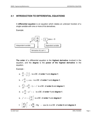
1. B5001- Engineering Mathematics DIFFERENTIAL EQUATION
4.1 INTRODUCTION TO DIFFERENTIAL EQUATIONS
A differential equation is an equation which relates an unknown function of a
single variable with one or more of its derivatives.
Example:
dy
x y cos x 0
dx
Independent variable Dependent variable
Derivative of y wrt x
The order of a differential equation is the highest derivative involved in the
equation, and the degree is the power of the highest derivative in the
equation.
Example :
dy 1 x
a. is a DE of order 1 and degree 1.
dx 1 y2
dy
b. x 2 y sin x is a DE of order 1 and degree 1.
dx
d2y dy
c. 4 2y x 2 is a DE of order 2 and degree 1.
dx 2 dx
dy
d. xy xy 2 x is a DE of order 1 and degree 1.
dx
2
2 dy
e. y 1 x is a DE of order 1 and degree 2
dx
2
d2 y dy
f. 2 10y cos 2x is a DE of order 2 and degree 2.
dx2 dx
Sa`adiah Saad JMSK, POLIMAS Page 1
2. B5001- Engineering Mathematics DIFFERENTIAL EQUATION
Example 1
State the dependent variable, the independent variable, the order and degree for each
differential equation.
ds s dm
i. ii. 2mn 0
dt t dn
2
dy 4 x ds
iii. iv. t2 sin t 0
dx x3 dt
dy dy
v. t2 1 yt vi. x xy y2 1
dt dx
d2y dy dv
vii. x 4 2 xy 0 viii. u3 1 uv2 u
dx 2 dx du
2
d2y dy d2y dy
ix. 3 2y 0 x. x 4 2 xy 0
dx 2 dx dx2 dx
Answer
Independent
Dependent Variable Order Degree
variable
i. s t 1 1
ii. m n 1 1
iii. y x 1 2
iv. s t 1 1
v. y t 1 1
vi. y x 1 1
vii. y x 2 1
viii. v u 1 1
ix. y x 2 2
x. y x 2 1
Sa`adiah Saad JMSK, POLIMAS Page 2
3. B5001- Engineering Mathematics DIFFERENTIAL EQUATION
4.2 Formation of Differential Equations
If y 10x2 A ; Differential Equation is formed when the arbitrary constant A
is eliminated from this equation.
Example 2
i. If y 10x2 A
Differentiate with respect to x,
dy
20 x
dx
dy
20x 0 Differential equation.
dx
ii. If y x Ax 2 ------
Differentiate with respect to x, gives,
dy
1 2 Ax -----
dx
y x
From , A 2
x
y x
Subtituting A 2
into
x
dy y x
Then, 1 2 2
x
dx x
y x
1 2
x
y
1 2 2
x
Multiply both sides with x.
dy
So, x x 2 y 2x
dx
dy
x 2y x
dx
Sa`adiah Saad JMSK, POLIMAS Page 3
4. B5001- Engineering Mathematics DIFFERENTIAL EQUATION
iii. If y Ax 2 Bx x -----
Differentiate with respect to x, gives,
dy
2 Ax B 1 -----
dx
dy
Differentiate with respect to x.
dx
d2y
2A -----
dx 2
1 d2y
From , A -----
2 dx 2
Substituting into to get B.
dy 1 d2y
2 x B 1
dx 2 dx2
d2y
x B 1
dx2
d2y dy
B x 1 -----
dx2 dx
Then, substitute and into .
1 d2y 2 d2y dy
y x x 2 1 x x
2 dx2 dx dx
1 2 d2y d2y dy
x x2 x x x
2 dx2 dx2 dx
1 2 d2y dy
x x
2 dx2 dx
Sa`adiah Saad JMSK, POLIMAS Page 4
5. B5001- Engineering Mathematics DIFFERENTIAL EQUATION
EXERCISE 1
Form differential equation of the following:
i. y x3 Ax 2 iv. y 4Bx A
ii. y Ax 2 7x v. y A sin 2 x B kos x
iii. y Dx 2 Ex vi. y Ce x
2 De x
Answer
dy dy
i. x2 3x 4 2( y x3 ) iv x 2 y 7x
dx dx
dy x2 d 2 y d2y
ii. y x v. 0
dx 2 dx2 dx2
d2y d2y
iii. 4y 0 vi y 0
dx 2 dx 2
4.3 SOLUTIONS OF FIRST ORDER DIFFERENTIAL EQUATIONS (DE)
We already know that DE is one that contains differential coefficient.
dy
Example: i. 4x - 1st order DE
dx
d2 y dy
ii.
2
2 4y 0 - 2nd order DE
dx dx
Sa`adiah Saad JMSK, POLIMAS Page 5
6. B5001- Engineering Mathematics DIFFERENTIAL EQUATION
dy
4.3.1 f(x) - Solve By Direct Integration; i.e. y f(x)dx
dx
dy
Example 3: Find the general solution of the DE 3x 2 sin2x
dx
Answer
dy cos2x
dx (3x 2 sin2x)dx so y = x3 c
dx 2
dy
Example 4: Find the particular solution of de 5 2x 3 , given the boundary
dx
2
conditions y 1 when x = 2 .
5
Answer
dy dy dy 3 2x 3 2x
5 2x 3 5 3 2x
dx dx dx 5 5 5
3 x2
Hence y x c
5 5
Substituting the boundary conditions;
7 3 22 7 6 4 7 6 4 5
(2) c c c= 1
5 5 5 5 5 5 5 5 5 5
3 x2
The particular solution, y x 1
5 5
Sa`adiah Saad JMSK, POLIMAS Page 6
7. B5001- Engineering Mathematics DIFFERENTIAL EQUATION
4.3.2 Solve By Variable Separable;
dy dy
4.3.2.1 f(y) - rearranged to give dx and then solve by direct
dx f(y)
dy
integration; i.e. dx
f(y)
dy
Example 5: Find the general solution of de 5 sin2 3y .
dx
Answer
dy dy
5 2
dx dx = 5
sin 3y sin2 3y
cot3y
x = 5 cosec 2 3y dy = 5[- ] +c
3
5
i.e. x = - cot3y +c
3
dy
Example 6: Find the particular solution of de (y 2 1) 3y given that y = 1 when
dx
x 13
6
Answer
(y 2 1) 1 y2 1 1 1
dy dx dx = dy dx = (y ) dy
3y 3 y 3 y
1 y2
x= ( - ln y) + c
3 2
Substituting y=1 and x 13 ;
6
Sa`adiah Saad JMSK, POLIMAS Page 7
8. B5001- Engineering Mathematics DIFFERENTIAL EQUATION
13 1 1 13 1
= ( - ln 1) + c c= - =2
6 3 2 6 6
1 2 1
The particular solution is x = y ln y 2
6 3
dy dy
4.3.2.2 f(x)g(y) - rearranged to give f(x)dx and then solve
dx g(y)
by direct integration
dy 2x3 1
Example 7: Solve
dx 3 2y
Answer
Separating the variables gives: (3 -2y)dy = (2x3 – 1)dx
x4
(3 2y)dy (2x 3 1)dx 3y - y 2 = x c
2
Example 8: The current in an electric circuit containing resistance R and inductance L
di
in series with a constant voltage source E is given by the de E L Ri .
dt
Solve the equation and find i in terms of time t given that when t = 0 and i
= 0.
Answer
di di 1
L E Ri dt
dt E-Ri L
Let u = E-Ri , du = -Rdi
1 du 1 1 1
- = dt - ln (E - Ri) = t c
R u L R L
Sa`adiah Saad JMSK, POLIMAS Page 8
9. B5001- Engineering Mathematics DIFFERENTIAL EQUATION
When t = 0, i= 0;
1 1
- ln E = c ; c=- ln E
R R
1 1 1
- ln (E - Ri) = t ln E
R L R
1 1 t
= ln E - ln (E - Ri) =
R R L
Rt Rt Rt
E Rt E E-Ri
ln ( )= eL e L E-Ri = Ee L
E-Ri L E-Ri E
Rt
E -
i = ( 1-e L )
R
Example 9: Solve the Des:
dy 2x xy dy y(2 3x)
a. 2
d.
dx y 1 dx x(1 3y)
ds s2 6s 9 dy 6t 2 2t 1
b. e.
dt t 2 dt cos y ey
dy sec h y
c.
dx 2 x
4.3.3 Homogeneneous First Order DEs
dy
An equation of the form P = Q , where P and Q are function of both x and y of the
dx
same degree – said to be homogenous in y and x.
Example;
Sa`adiah Saad JMSK, POLIMAS Page 9
10. B5001- Engineering Mathematics DIFFERENTIAL EQUATION
f(x,y) Homogeneous degree
1 x2 + 3xy + y2 yes 2
x 3y
2 yes 1
2x y
4 x 2 3y 2
3 yes 2
2 xy
x2 y y–1
4 no
2 x2 y2 x-2
dy
Procedure to solve DE of the form P =Q
dx
dy dy Q
i. Rearrange P = Q into the form =
dx dx P
dy dv
ii. Make the substitution y =vx, from = v (1) + x , by the product rule.
dx dx
dy dy Q
Substitute for both y and in the equation = . Simplify, by
iii. dx dx P
cancelling, and on equation result in which the variables are separable.
iv. Separate the variable and solve as direct integrating.
y
v. Substitute v = to solve in terms of the original variables.
x
dy
Example 10: Solve the DE y - x = x , given x = 1 when y = 2.
dx
Answer
dy y - x
i. Rearranging; =
dx x
dy dv
ii. Let y = vx, =v+x
dx dx
dy dv v x - x
iii. Substitute for both y and gives: v + x =
dx dx x
Sa`adiah Saad JMSK, POLIMAS Page 10
11. B5001- Engineering Mathematics DIFFERENTIAL EQUATION
dv x(v - 1) dv
v+x = x v-1-v
dx x dx
dv dx
x -1 dv=- v = - ln x +c
dx x
y
= - ln x +c Subtitute x =1 and y = 2
x
2
c c=2
1
y
= - ln x + 2 or y = - x ( ln x - 2 )
x
dy x2 y2
Example 11: Find the particular solution of DE; x given the boundary
dx y
conditions that y = 4 when x = 1.
Answer
dy x2 y2 dy x2 y2
i. Rearranging; x
dx y dx yx
dy dv
ii. Let y = vx, =v+x
dx dx
dv x2 + v 2 x2 x2 (1 + v 2 ) (1 + v 2 )
iii. v+x =
dx vx2 vx2 v
dv (1 + v 2 ) 1 + v2 v2 1
x v
dx v v v
1
vdv = dx
x
v2
= ln x + c
2
Sa`adiah Saad JMSK, POLIMAS Page 11
12. B5001- Engineering Mathematics DIFFERENTIAL EQUATION
y2
2
= ln x + c y2 2x 2 (ln x c)
2x
16
c c=8 y 2 = 2x 2
(lnx + 8)
2
4.3.4 Linear First Order DEs
dy
If P = P(x) and Q = Q(x) are functions of x only, then + Py = Q is called a linear
dx
differential equation order 1. We can solve these linear DEs using an integrating
factor. For linear DEs of order 1, the integrating factor is: e∫Pdx
The solution for the DE is given by multiplying y by the integrating factor (on the left)
and multiplying Q by the integrating factor (on the right) and integrating the right side
with respect to x, as follows:
y eò Q eò
Pdx Pdx
=
ò +K
dy 3
Example 12: Solve for - y = 7.
dx x
Answer
dy 3 3
- y = 7. then P(x) = - and Q(x) = 7
dx x x
Now for the integrating factor:
3 3
ò Pdx = e ò - x dx = e ò - x dx = e- 3 ln x = x- 3
IF= e
For the left hand side of the formula
Sa`adiah Saad JMSK, POLIMAS Page 12
13. B5001- Engineering Mathematics DIFFERENTIAL EQUATION
ye ò Qe ò
Pdx Pdx
=
ò dx
we have ye∫Pdx = yx-3
For the right hand of the formula, Q = 7 and the IF = x-3, so:
Qeò
Pdx - 3
= 7x
Qe ò
Pdx 7 -2
ò ò 7x
- 3
Applying the outer integral: dx = dx = - x +K
2
ye ò Qe ò
Pdx Pdx
Now, applying the whole formula; =
ò dx
- 3 7 -2
we have ; yx =- x +K
2
7 3
Multiplying throughout by x3 gives: y = - x + Kx
2
dy
Example 13: Solve + (cot x)y = cos x
dx
Answer
dy
+ (cot x)y = cos x
dx
Here, then P(x) = cot x and Q(x) = cos x
Determine
ò Pdx = ò cot xdx = lnsin x
IF = e
ò Pdx = eln sin x = sin x
ò Pdx = cos x sin x
Now Qe
Apply the formula:
ye ò Qe ò
Pdx cot xdx
=
ò dx
Sa`adiah Saad JMSK, POLIMAS Page 13
14. B5001- Engineering Mathematics DIFFERENTIAL EQUATION
y sin x =
ò cos x sin xdx
The integral needs a simple substitution: u = sin x, du = cos x dx
2
sin x
y sin x = +K
2
Divide throughout by sin x:
sinx K sinx
y= + = + K cosecx
2 sinx 2
- 3x
Example 14: Solve dy + 3ydx = e dx
Answer
Dividing throughout by dx to get the equation in the required form, we get:
dy - 3x
+ 3y = e
dx
In this example, P(x) = 3 and Q(x) = e-3x.
Now e∫Pdx = e∫3dx = e3x
and
Qe ò
Pdx
òe ò 1dx = x
- 3x 3x
= e dx =
ò Pdx
Qe ò
Pdx
Using ye =
ò dx + K , we have:
ye3x = x + K
or we could write it as:
x +K
y=
3x
e
Example 15: Solve 2(y - 4x2)dx + x dy = 0
Answer
Sa`adiah Saad JMSK, POLIMAS Page 14
15. B5001- Engineering Mathematics DIFFERENTIAL EQUATION
We need to get the equation in the form of a linear DE of order 1.
Expand the bracket and divide throughout by dx:
2 dy
2y - 8x + x = 0
dx
Rearrange:
dy 2
x + 2y = 8x
dx
Divide throughout by x:
dy 2
+ y = 8x
dx x
2
Here, P(x) = and Q(x) = 8x
x
2
ò Pdx ò x dx 2 ln x ln x
2
2
IF = e = e = e = e = x
Now Qe ò
Pdx 2 3
= 8xx = 8x
Applying the formula:
ye ò Qeò
Pdx Pdx
=
ò dx + K
ò
2 3 4
gives: yx = 8x dx + K = 2x + K
2 K
Divide throughout by x2: y = 2x +
2
x
dy 6 x
Example 16: Solve x - 4y = x e
dx
Answer
Divide throughout by x:
dy 4 5 x
- y= x e
dx x
4 5 x
Here, P(x) = - and Q(x) = x e
x
Sa`adiah Saad JMSK, POLIMAS Page 15
16. B5001- Engineering Mathematics DIFFERENTIAL EQUATION
4
ò - dx - 4
IF = e ò
P(x)dx ln x - 4
= e x = e = x
Now Qe
ò P(x)dx = x5 ex x- 4 = xex
ye ò Qeò
Pdx Pdx
Applying the formula: =
ò dx + K gives
ò
- 4 x
yx = xe dx + K
This requires integration by parts, with
x
u= x dv=e
x
du = dx v=e
- 4 x x
So yx = xe - e + K
5 x 4 x 4
Multiplying throughout by x4 gives: y = x e - x e +Kx
dy x
Example 17: Solve e 2y , x 0 , subject to the initial condition y = 2
dx
when x = 0
Answer
The differential equation can be expressed in the proper form by adding
2y to both sides:
dy x
2y e for x 0
dx
x
We have P(x) = 2 and Q(x) = e
P(x)dx 2dx
An integrating factor is given by IF = e e e2x for x 0
Sa`adiah Saad JMSK, POLIMAS Page 16
17. B5001- Engineering Mathematics DIFFERENTIAL EQUATION
Next, use the first-order linear differential equation theorem, where IF =
x
e 2 x and Q(x) = e , to find y:
1
y= 2x
e2x e x dx C
e
1
= 2x
ex C e x
e 2x
C for x 0
e
To find C, insert y = 2 when x = 0, to obtain C = 1
x 2x
Thus y = e e , x 0
dy 2xy
Example 18: Solve sin x with y = 1 when x = 0
dx 1 x2
Answer
2x
P(x) = ; Q(x) = sin x
1 x2
2x
dx
2 1)
IF = e 1 x2 = e ln(x x2 1
1
y= 2
(x 2 1)sin xdx C
1 x
1
= 2
x 2 sin xdx sin xdx C
1 x
1
= 2
2x sin x (2 x 2 )cos x cos x C
1 x
Sa`adiah Saad JMSK, POLIMAS Page 17
18. B5001- Engineering Mathematics DIFFERENTIAL EQUATION
1
= 2
2x sin x (1 x 2 )cos x C
1 x
Since y = 1 when x = 0,
1
1= 0 1 C implies C = 0
1
1
y= 2
2xsinx +(1- x 2 )cosx
1+ x
Example 19:
dy
a. Solve the DE = sec θ + y tan θ , given the boundary conditions y=1 when θ = 0.
dθ
[Ans: y = (θ + 1) sec θ]
dy 5 c
b. Solve the DE t -5 t = -y . [ ans: y t ]
dt 2 t
c. Consider a simple electric circuit with the resistance of 3 an inductance of 2H. If a
battery gives a constant voltage of 24V and the switch is closed when t = 0, the
current, I(t), after t seconds is given by
dI 4
+ t = 15, I(0) = 0
dt 3
4
45 t
i) Obtain I(t) [ans: I(t) (1 e 3 )]
4
ii) Determine the difference in the amount of current flowing through the circuit from
the fourth to eight seconds. Give your answer to 3 d.p.
[ans: 0.05 A]
iii) If the current is allowed to flow through the circuit for a very long period of time,
estimate I(t).
Sa`adiah Saad JMSK, POLIMAS Page 18
19. B5001- Engineering Mathematics DIFFERENTIAL EQUATION
45
[ans: A]
4
4.4 SECOND ORDER DIFFERENTIAL EQUATION
The general form of the second order differential equation with constant coefficients is
d2y dy
a +b + cy = Q( x )
dx 2 dx
where a, b, c are constants with a > 0 and Q(x) is a function of x only.
4.4.1 Homogeneous Equation
In this section, most of our examples are homogeneous 2nd order linear DEs (that is, with
Q(x) = 0):
d 2y dy
a +b + cy = 0 , where a, b, c are constants.
dx 2 dx
Method of Solution
The equation am2 + bm + c = 0 is called the Auxiliary Equation (A.E.) (or
Characteristic Equation)
The general solution of the differential equation depends on the solution of the A.E. To
find the general solution, we must determine the roots of the A.E. The roots of the A.E.
are given by the well-known quadratic formula:
m= -b ± b2 - 4ac
2a
Sa`adiah Saad JMSK, POLIMAS Page 19
20. B5001- Engineering Mathematics DIFFERENTIAL EQUATION
Summary:
If Differential Equation: ay'' + by' + c = 0 and Associated auxiliary equation is:
am2 + bm + c = 0
Nature of roots Condition General Solution
4.4.1. Real and distinct roots,
b2 − 4ac > 0 y = Aem1x + Bem2x
m1, m2
4.4.2. Real and equal roots, m b2 − 4ac = 0 y = emx(A + Bx)
4.4.3. Complex roots
m1 = α + jω b2 − 4ac < 0 y = eαx(A cos ωx + B sin ωx)
m1 = α − jω
Example 20
2
d i di
The current i flowing through a circuit is given by the equation + 60 + 500i = 0 ,
dt dt
Solve for the current i at time t > 0.
Answer
The auxiliary equation arising from the given differential equations is:
2
A.E.: m + 60m + 500 = 0 = (m + 50)(m + 10) = 0
So m = - 50 and m = - 10 and
1 2
We have 2 distinct real roots, so we need to use the first solution from the table above
(y = Aem1x + Bem2x), but we use i instead of y, and t instead of x.
Sa`adiah Saad JMSK, POLIMAS Page 20
21. B5001- Engineering Mathematics DIFFERENTIAL EQUATION
- 10t - 50t
So i = Ae + Be
- 10t - 50t
We could have written this as: i= C e + C e
1 2
Since we have 2 constants of integration. We would be able to find these constants if
we were given some initial conditions.
Example 21
Solve the following equation in which s is the displacement of a object at time t.
2
d s ds ds
- 4 + 4s = 0 , given that s = 1, = 3 when t = 0
2 dt dt
dt
(That is, the object's position is 1 unit and its velocity is 3 units at the beginning of the
motion.)
Answer
The auxiliary equation for our differential equation is:
2 2
A.E. m - 4m + 4 = 0 = (m - 2) = 0
In this case, we have: m = 2 (repeated root or real equal roots)
We need to use the second form from the table above (y = emx(A + Bx)), and once again
use the correct variables (t and i, instead of x and y).
2t
So S(t) = ( A + Bt )e .
Now to find the values of the constants:
s(0) = 1 Þ A = 1
2t
So we can write S(t) = (1+ Bt )e
' 2t 2t
S (t) = 2(1+Bt)e +Be
s '(0) = 3 Þ 2 + B = 3 Þ B = 1
Sa`adiah Saad JMSK, POLIMAS Page 21
22. B5001- Engineering Mathematics DIFFERENTIAL EQUATION
2t
So s t)
( =(1+ t )e
The graph of our solution is as follows:
Example 22
d 2y dy
Solve the equation - 2 + 4y = 0
2 dx
dx
Answer
2
This time the auxiliary equation is: m - 2m + 4 = 0
Solving for m, we find that the solutions are a complex conjugate pair:
m = 1- j 3 and m = 1 + j 3
1 2
The solution for our DE, using the 3rd type from the table above:
y = eαx(A cos ωx + B sin ωx)
x
we get: y(x) = e (Acos 3 x +Bsin 3 x)
Sa`adiah Saad JMSK, POLIMAS Page 22
23. B5001- Engineering Mathematics DIFFERENTIAL EQUATION
Example 23
In a RCL series circuit, R = 10 Ω, C = 0.02 F, L = 1 H and the voltage source is E = 100
V. Solve for the current i(t) in the circuit given that at time t = 0, the current in the circuit
is zero and the charge in the capacitor is 0.1 C.
[Note: Damping and the Natural Response in RLC Circuits
Consider a series RLC circuit (one that has a resistor, an inductor and a capacitor) with
a constant driving electro-motive force (emf) E. The current equation for the circuit is
di 1 di 1
L + Ri + ò idt = E or L + Ri + q = E
dt C dt C
Differentiating, we have
2
d i di 1
L +R + i = 0 ; This is a second order linear homogeneous equation.]
dt
2 dt C
Answer
d 2i + 10 di + 50i = 0
dt 2 dt
AE : m2 + 10m + 50 = 0 ,
Sa`adiah Saad JMSK, POLIMAS Page 23
24. B5001- Engineering Mathematics DIFFERENTIAL EQUATION
The factors are: m = - 5 - j5 and m = - 5 + j5
1 2
So, i = e- 5t ( Acos5t + B sin5t ) ; éù
i
êú
ëû
= A = 0 ; (This means at t = 0, i = A = 0 in this
t= 0
case.)
Then i = e- 5t B sin5t , We need to find the value of B.
Differentiating gives:
di - 5t - 5t - 5t
= e (5B cos5t ) + (B sin5t )(- 5e ) = 5Be (cos5t - sin5t )
dt
di
At t = 0, = 5B
dt
di
Returning to equation + 10i + 50q = 100
dt
di di
Now, at time t = 0, + 10(0) + 50(0.1) = 100 ; So = 95 = 5B , so B = 19.
dt t = 0 dt t = 0
-5t
Therefore, i = 19e sin5t
Sa`adiah Saad JMSK, POLIMAS Page 24