Downloaded 13 times
![Chapter 4
Multiple Integrals
4.1 Double Integral Over Rectangular Regions
4.1.1 Quick Review of the De…nite Integral
This review is intended more to introduce the notation we will use than to cover
the topic of the de…nite integral. It is assumed the student is already familiar
with it. If this is not the case, students should …rst review the de…nite integral
in any calculus book, or using my notes on the web site for the class.
The de…nite integral was de…ned when we were trying to solve the area
problem. Given a function y = f (x) de…ned for a x b, we wanted to …nd
the area between the graph of y = f (x), the x-axis, and the vertical lines x = a
and x = b. We begin by dividing the interval [a; b] into n subintervals [xi 1 ; xi ],
i = 1::n, of equal length. Let x denote the length of each subinterval. Clearly,
x = b na . In each subinterval [xi 1 ; xi ], we pick a point we denote xi . We
form the Riemann sum
Xn
f (xi ) x
i=1
The de…nite integral was de…ned to be
Zb n
X
f (x) dx = lim f (xi ) x
n!1
a i=1
In the case that f (x) 0 on [a; b], the integral corresponds to the area below
the graph (see …gure 4.1).
4.1.2 Double Integrals and Volumes
For the de…nite integrals we reviewed above, the function we were integrating
was a function of one variable. That is a function of the form f : R ! R. Hence,
its domain is either R or a subset of R. When we integrate, we also integrate
199](https://image.slidesharecdn.com/multipleintegrals-121215113224-phpapp02/85/Multiple-integrals-1-320.jpg)
![Chapter 4
Multiple Integrals
4.1 Double Integral Over Rectangular Regions
4.1.1 Quick Review of the De…nite Integral
This review is intended more to introduce the notation we will use than to cover
the topic of the de…nite integral. It is assumed the student is already familiar
with it. If this is not the case, students should …rst review the de…nite integral
in any calculus book, or using my notes on the web site for the class.
The de…nite integral was de…ned when we were trying to solve the area
problem. Given a function y = f (x) de…ned for a x b, we wanted to …nd
the area between the graph of y = f (x), the x-axis, and the vertical lines x = a
and x = b. We begin by dividing the interval [a; b] into n subintervals [xi 1 ; xi ],
i = 1::n, of equal length. Let x denote the length of each subinterval. Clearly,
x = b na . In each subinterval [xi 1 ; xi ], we pick a point we denote xi . We
form the Riemann sum
Xn
f (xi ) x
i=1
The de…nite integral was de…ned to be
Zb n
X
f (x) dx = lim f (xi ) x
n!1
a i=1
In the case that f (x) 0 on [a; b], the integral corresponds to the area below
the graph (see …gure 4.1).
4.1.2 Double Integrals and Volumes
For the de…nite integrals we reviewed above, the function we were integrating
was a function of one variable. That is a function of the form f : R ! R. Hence,
its domain is either R or a subset of R. When we integrate, we also integrate
199](https://image.slidesharecdn.com/multipleintegrals-121215113224-phpapp02/75/Multiple-integrals-1-2048.jpg)
![200 CHAPTER 4. MULTIPLE INTEGRALS
Figure 4.1: Approximating the area below a curve
over portions of its domain, most of the time over closed and bounded portions
of its domain, that is over intervals. The functions we are about to learn how
to integrate are functions of two variables or more. Let us focus on functions
on two variables for a while, that is on functions of the form f : R2 ! R.
The domain of such functions is a subset of R2 that is the plane. We will
be integrating over closed and bounded regions of the plane. The problem is
that there are many possibilities for such regions ranging from a square or a
rectangle to more complicated shapes. The region of integration is an added
di¢ culty when dealing with multiple integrals, a di¢ culty we do not have for
functions of one variable since we are always integrating over an interval. We
will …rst consider integrals over a rectangular region. These are very simple.
Then, we will look at more complicated regions.
In spite of this added di¢ culty, double integrals are de…ned in a manner
similar to that of de…nite integrals. Suppose that we are given a function f (x; y)
de…ned over a closed rectangle
R = (x; y) 2 R2 j a x b; c y d
= [a; b] [c; d]
As in the case of functions of one variable, we will …rst assume that f (x; y) 0
on R. Let S be the solid which lies above R and below the graph of f . In other
words,
S = (x; y; z) 2 R3 j 0 z f (x; y) ; (x; y) 2 R
We wish to …nd V , the volume of S (see …gure 4.2).
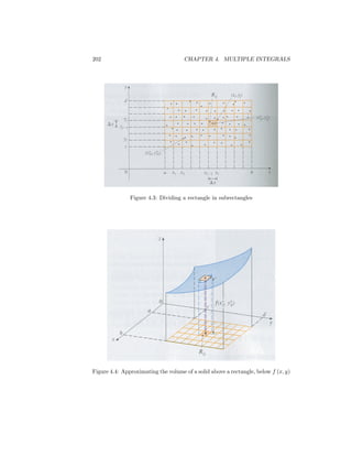
We begin by dividing R into subrectangles. For this, we divide the interval
[a; b] into m subintervals [xi 1 ; xi ], i = 1::m, of equal length x = bma . We also
divide the interval [c; d] into n subintervals [yj 1 ; yj ], j = 1::n, of equal length](https://image.slidesharecdn.com/multipleintegrals-121215113224-phpapp02/85/Multiple-integrals-2-320.jpg)
![4.1. DOUBLE INTEGRAL OVER RECTANGULAR REGIONS 201
Figure 4.2: Solid above R below f (x; y)
d c
y= n . This way, we obtain the subrectangles
Rij = (x; y) 2 R2 j xi 1 x xi ; yj 1 y yj
= [xi 1 ; xi ] [yj 1 ; yj ]
The area of each Rij is A = x y (see …gure 4.3).
Next, in each subrectangle Rij , we pick a point denoted xij ; yij . We form
the box with base Rij and height f xij ; yij . Its volume is f xij ; yij A (see
…gure 4.4).
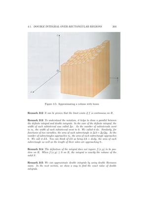
We can approximate the volume of S by adding the volume of each box
obtained (see …gure 4.5). In other words, we have
m n
XX
V t f xij ; yij A
i=1 j=1
Remark 310 The above sum is called a double Riemann sum.
As in the case of functions of one variable, our approximation should get
better the larger m and n are . We de…ne the double integral of f over R to be
De…nition 311 The double integral of f (x; y) over the rectangle R is:
ZZ m n
XX
f (x; y) dA = lim f xij ; yij A
m;n!1
R i=1 j=1
providing the limit exists.](https://image.slidesharecdn.com/multipleintegrals-121215113224-phpapp02/85/Multiple-integrals-3-320.jpg)
![204 CHAPTER 4. MULTIPLE INTEGRALS
4.2 Iterated Integrals Over Rectangular Regions
Let f (x; y) be a function which is continuous on R = [a; b] [c; d]. When we
Rd
write c f (x; y) dy, we mean that x is held as a constant and we integrate with
respect to y. This is similar to partial di¤erentiation with respect to y, in the
sense that x is held as a constant in both cases. This process is called partial
integration with respect to y.
R2
Example 316 Find 1 x2 ydy
Z 2 Z 2
x2 ydy = x2 ydy since x is a constant
1 1
" 2
#
2 y2
= x
2 1
1
= x2 2
2
3 2
= x
2
R
Example 317 Find 0
sin x sin ydy
Z Z
sin x sin ydy = sin x sin ydy
0 0
= sin x [ cos yj0 ]
= sin x [ cos + cos 0]
= 2 sin x
Rd
Remark 318 When we compute an integral of the form f (x; y) dy, we will c
Rd
be left with a function of x. Call it A (x). In other words, A (x) = c f (x; y) dy.
Rb
We can now integrate A (x) with respect to x between a and b. We get a A (x) dx.
In fact, we have
Z b Z b "Z d #
A (x) dx = f (x; y) dy dx (4.1)
a a c
De…nition 319 An integral like the one on the right side of equation 4.1 is
called an iterated integral.
Remark 320 Usually, we omit the bracket, thus
Z b "Z d # Z bZ d
f (x; y) dy dx = f (x; y) dydx (4.2)
a c a c
To compute it, we integrate in two steps. First, we evaluate the integral inside,
the one with respect to y; holding x as a constant. This will give us a function
of x. We then integrate that function with respect to x.](https://image.slidesharecdn.com/multipleintegrals-121215113224-phpapp02/85/Multiple-integrals-6-320.jpg)
![206 CHAPTER 4. MULTIPLE INTEGRALS
Theorem 324 (Fubini’ Theorem) Suppose that f (x; y) is continuous on
s
the rectangle R = [a; b] [c; d]. Then
ZZ Z bZ d Z dZ b
f (x; y) dA = f (x; y) dydx = f (x; y) dxdy
a c c a
R
Remark 325 Note that the order of integration does not matter. We can …rst
integrate with respect to y, then to x: We can also do the reverse. Make sure
you use the correct limits of integration. For the dx integral, the limits must be
for the x variable: For the dy integral, the limits must be for the y variable.
ZZ
Example 326 Compute x 3y 2 dA where R = (x; y) 2 R2 j 0 x 2; 1 y 2 .
R
Method 1: Using Fubini’ theorem, we get
s
ZZ Z 2 Z 2
x 3y 2 dA = x 3y 2 dxdy
1 0
R
Z " 2
#
2
x2
= 3xy 2 dy
1 2 0
Z 2
= 2 6y 2 dy
1
2
= 2y 2y 3 1
= (4 16) (2 2)
= 12
Method 2: We can also use Fubini’ theorem, but with the opposite order of
s
integration. We should get the same answer.
ZZ Z 2Z 2
2
x 3y dA = x 3y 2 dydx
0 1
R
Z 2 h i
2
= xy y3 1
dx
0
Z 2
= [(2x 8) (x 1)] dx
0
Z 2
= (x 7) dx
0
2
x2
= 7x
2 0
= 2 14
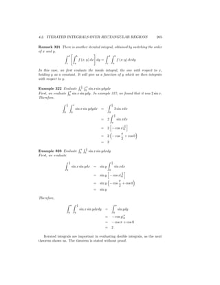
= 12](https://image.slidesharecdn.com/multipleintegrals-121215113224-phpapp02/85/Multiple-integrals-8-320.jpg)
![208 CHAPTER 4. MULTIPLE INTEGRALS
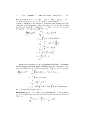
Figure 4.6: Graph of f (x; y) = x2 2y 2 + 16
R R
Example 329 Evaluate 02 0 sin x sin ydydx
From the proposition, we have
Z 2
Z Z 2
Z
sin x sin ydydx = sin xdx sin ydy
0 0
h0 i 0
= cos xj0 [ cos yj0 ]
2
= [1] [2]
= 2
4.2.1 Summary
We list important points covered in this section.
It is important to understand that in addition to …nding antiderivative, the
is an additional di¢ culty with multiple integrals: the region of integration.
For the de…nite integral, that is the integral of a function of one variable,
the region of integration was an interval. For multiple integrals, the region
of integration will be a subset of the plane for functions of two variables,
or a subset of space for functions of three variables. There are many more
possibilities of such regions. This section focused on rectangular regions.](https://image.slidesharecdn.com/multipleintegrals-121215113224-phpapp02/85/Multiple-integrals-10-320.jpg)
![4.2. ITERATED INTEGRALS OVER RECTANGULAR REGIONS 209
We learned to compute iterated integrals, that is integrals of the form
RbRd RdRb
a c
f (x; y) dydx or c a f (x; y) dxdy. Note there are two kinds, de-
pending on the order of integration.
We learned to compute double integrals over a rectangular region, that is
ZZ
integrals of the form f (x; y) dA where R = [a; b] [c; d].
R
A double integral is evaluated in terms of iterated integrals. More pre-
cisely, if R = [a; b] [c; d], then Fubini’ theorem tells us that
s
ZZ Z b Z d Z d Z b
f (x; y) dA = f (x; y) dydx = f (x; y) dxdy
a c c a
R
Note that we can switch the order of integration when the region is a
rectangle.
ZZ
If the graph of z = f (x; y) is above the xy-plane then f (x; y) dA is
R
the volume of the solid with cross section R, between the xy-plane and
z = f (x; y).
4.2.2 Assignment
Odd numbers 1-27 at the end of 12.1 in your book.](https://image.slidesharecdn.com/multipleintegrals-121215113224-phpapp02/85/Multiple-integrals-11-320.jpg)

This document discusses double integrals and their use in calculating volumes. It begins by introducing double integrals as a way to calculate the volume of a solid bounded above by a function f(x,y) over a rectangular region. It then discusses using iterated integrals to evaluate double integrals by first integrating with respect to one variable and then the other. Finally, it provides examples of using double integrals and iterated integrals to calculate volumes.