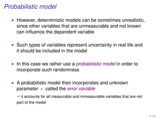
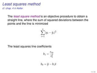
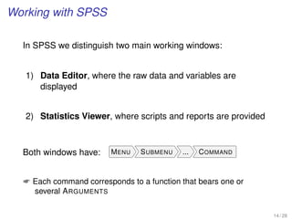
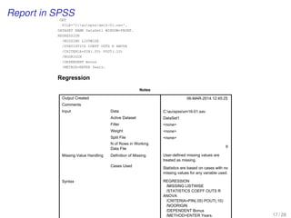
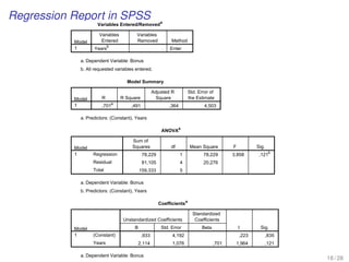
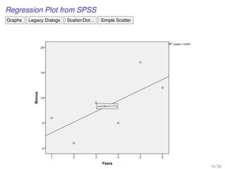
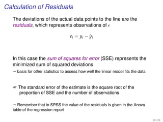
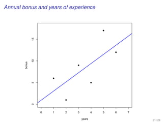
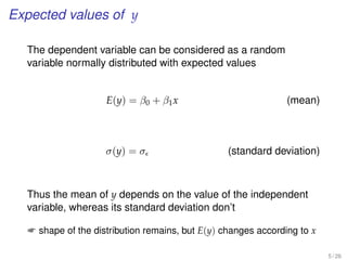
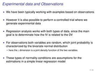
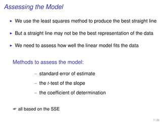
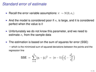
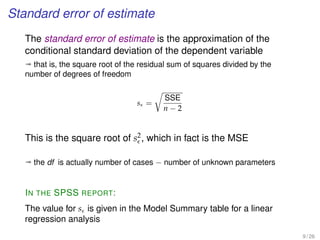
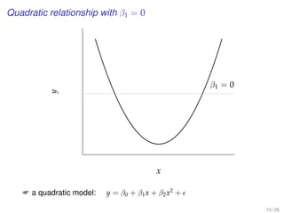
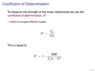
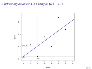
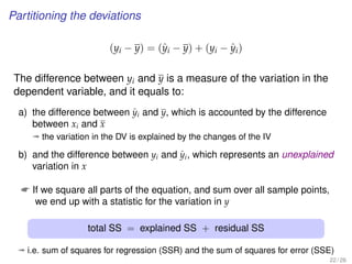
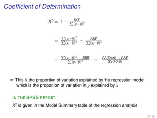
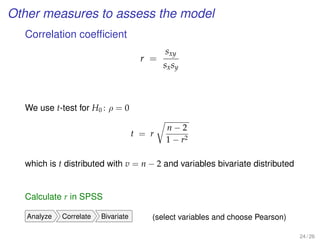
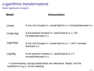
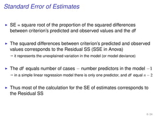
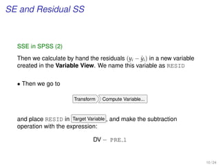
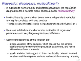
This document provides an overview of lectures for a Business Statistics II course between weeks 11-19. It covers topics like simple regression analysis, estimation in regression models, and assessing regression models. Key points include using least squares to estimate regression coefficients, calculating residuals, and evaluating fit using measures like the coefficient of determination and standard error of the estimate. Examples are provided to illustrate simple linear regression analysis.
![EXAMPLE-DO-IT-YOUR-SELF
[A predicted variable and a predictor variable]
We do examples with random numbers...
26 / 28](https://image.slidesharecdn.com/business-statistics-ii-aarhus-bss-170814111356/85/Business-statistics-ii-aarhus-bss-26-320.jpg)


![EXAMPLE-DO-IT-YOUR-SELF
[A predicted variable and a predictor variable]
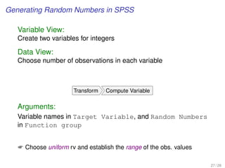
Data generation in SPSS
• Choose your DV and IV, and number of observations. Then generate
uniform random numbers:
Transform Compute Variable...
• Variable names in Target Variable , and Random Numbers in Function group
• Select Rv.Uniform in Functions and Special Variables , and then establish the
range of the observation values in Numeric Expression
9 / 31](https://image.slidesharecdn.com/business-statistics-ii-aarhus-bss-170814111356/85/Business-statistics-ii-aarhus-bss-63-320.jpg)
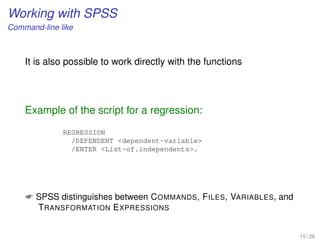
![EXAMPLE-DO-IT-YOUR-SELF
[A predicted variable and a predictor variable]
Confidence intervals of the regression model in SPSS
• We perform the linear regression analysis
Analyze Regression Linear
• Individual confidential intervals are given in this command, where in the
bottom Save we select in Prediction Intervals
– the Individual option for Prediction Interval
– the Mean option for the Confidential Interval Estimator
Both at the usual 95% value
10 / 31](https://image.slidesharecdn.com/business-statistics-ii-aarhus-bss-170814111356/85/Business-statistics-ii-aarhus-bss-64-320.jpg)
![EXAMPLE-DO-IT-YOUR-SELF
[A predicted variable and a predictor variable]
Confidence intervals of the regression model in SPSS (2)
• Since we have chosen Save , the confidential interval values are saved in
the Data Editor
ª here LMCI [UMCI] and LICI [UICI] stand respectively for Lower
[Upper] Mean and Individual Confidence Interval
The Variable View in the Data Editor gives the labels of the new variables
11 / 31](https://image.slidesharecdn.com/business-statistics-ii-aarhus-bss-170814111356/85/Business-statistics-ii-aarhus-bss-65-320.jpg)
![EXAMPLE-DO-IT-YOUR-SELF
[A predicted variable and a predictor variable]
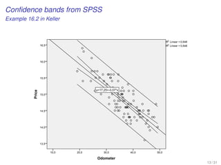
Visualizing confidence intervals in SPSS
• The visualization of both types of confidence intervals are possible after we
plotted the variables
Graphs Legacy Dialogs Scatter/Dot... Simple Scatter
• From Elements Fit Line at Total of the graph Chart Editor, we look in the
tab Fit Line (Properties) the options Mean and Individual in the
Confidential Intervals section for the two CI estimators
12 / 31](https://image.slidesharecdn.com/business-statistics-ii-aarhus-bss-170814111356/85/Business-statistics-ii-aarhus-bss-66-320.jpg)
![EXAMPLE-DO-IT-YOUR-SELF
[A predicted variable and a predictor variable]
Predict new observations in SPSS
• To forecast new observations, first we need to put the value in the
dependent variable of the Data Editor
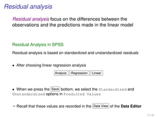
• Then we choose a linear regression analysis
Analyze Regression Linear
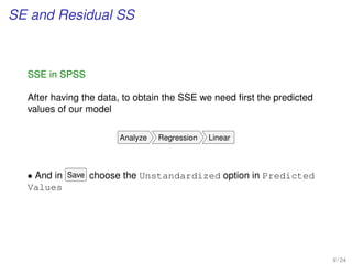
• And, after we press the Save bottom, we select the Unstandardized
option in Predicted Values
14 / 31](https://image.slidesharecdn.com/business-statistics-ii-aarhus-bss-170814111356/85/Business-statistics-ii-aarhus-bss-68-320.jpg)

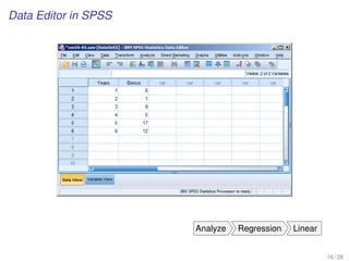
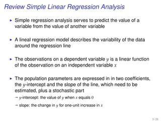
![Step-by-step simple linear regression analysis
EXAMPLE
[Population and avg. Household Size in Global Cities]
Be aware that in this case the model is chosen in advance, and
we adopt a linear relationship between two variables
18 / 24](https://image.slidesharecdn.com/business-statistics-ii-aarhus-bss-170814111356/85/Business-statistics-ii-aarhus-bss-103-320.jpg)
![Step-by-step simple linear regression analysis
EXAMPLE
[Population and avg. Household Size in Global Cities]
1. Determine the response and the explanatory variables
2. Visualize the data through a scatter plot
3. Perform basic descriptive statistics
19 / 24](https://image.slidesharecdn.com/business-statistics-ii-aarhus-bss-170814111356/85/Business-statistics-ii-aarhus-bss-104-320.jpg)
![Step-by-step simple linear regression analysis
EXAMPLE
[Population and avg. Household Size in Global Cities]
4. Estimate the coefficients (intercept and slope)
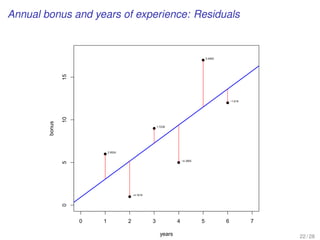
5. Compute the fitted values and the residuals
6. Obtain the sum of squares for errors (Residual SS)
20 / 24](https://image.slidesharecdn.com/business-statistics-ii-aarhus-bss-170814111356/85/Business-statistics-ii-aarhus-bss-105-320.jpg)
![Step-by-step simple linear regression analysis
EXAMPLE
[Population and avg. Household Size in Global Cities]
7. Estimate the coefficients (intercept and slope)
a) standard error of estimate
b) test of the slope
c) coefficient of determination
21 / 24](https://image.slidesharecdn.com/business-statistics-ii-aarhus-bss-170814111356/85/Business-statistics-ii-aarhus-bss-106-320.jpg)
![Step-by-step simple linear regression analysis
EXAMPLE
[Population and avg. Household Size in Global Cities]
8. Perform the regression diagnostics
a) confidence regions for individual prediction intervals
b) confidence regions for the average prediction interval
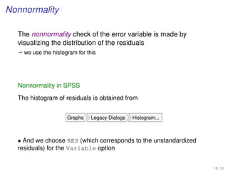
9. Make a residual analysis
a) nonnormality, heteroskedasticity, nonindependence errors
22 / 24](https://image.slidesharecdn.com/business-statistics-ii-aarhus-bss-170814111356/85/Business-statistics-ii-aarhus-bss-107-320.jpg)
![Step-by-step simple linear regression analysis
EXAMPLE
[Population and avg. Household Size in Global Cities]
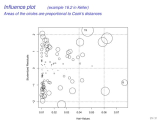
10. Detect outliers and influential observations
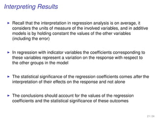
11. Interpret the results
12. Draw the conclusions
23 / 24](https://image.slidesharecdn.com/business-statistics-ii-aarhus-bss-170814111356/85/Business-statistics-ii-aarhus-bss-108-320.jpg)

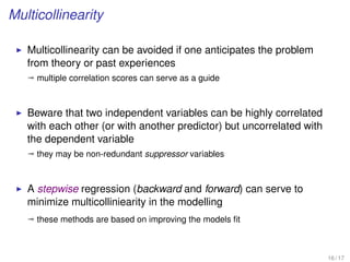
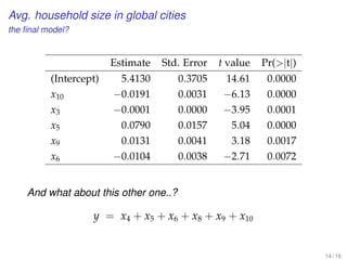
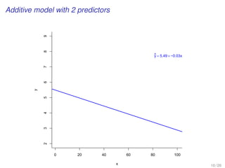
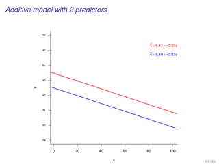
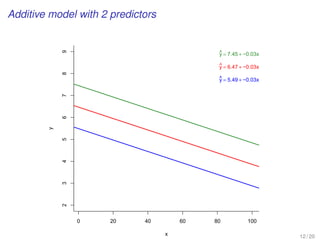
![Multiple regression analysis
WORKING EXAMPLE
[Prediction of avg. Household Size in Global Cities]
Multiple regression analysis using globalcity-multiple.sav
17 / 17](https://image.slidesharecdn.com/business-statistics-ii-aarhus-bss-170814111356/85/Business-statistics-ii-aarhus-bss-125-320.jpg)

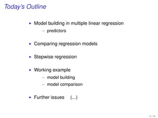
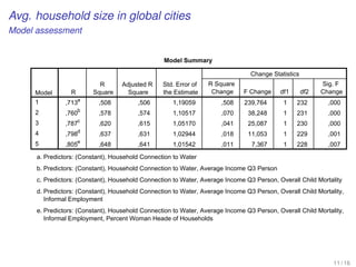
![WORKING EXAMPLE
[Average Household Size in Global Cities]
Model Building
(Data in globalcity-multiple.sav)
10 / 16](https://image.slidesharecdn.com/business-statistics-ii-aarhus-bss-170814111356/85/Business-statistics-ii-aarhus-bss-135-320.jpg)
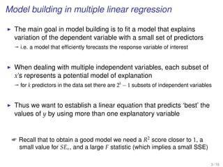
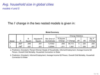
![WORKING EXAMPLE
[Average Household Size in Global Cities]
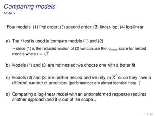
Comparing nested models
12 / 16](https://image.slidesharecdn.com/business-statistics-ii-aarhus-bss-170814111356/85/Business-statistics-ii-aarhus-bss-137-320.jpg)
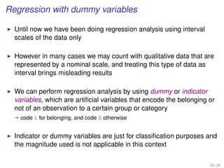
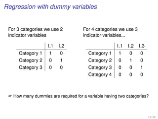
![Dummies with command-line
We need to create a number of dummy variables according to
the existing number of categories.
Syntax in SPSS:
RECODE varlist_1 (oldvalue=newvalue) ... (oldvalue=newvalue)
[INTO varlist_2].
[/varlist_n].
EXECUTE.
20 / 20](https://image.slidesharecdn.com/business-statistics-ii-aarhus-bss-170814111356/85/Business-statistics-ii-aarhus-bss-161-320.jpg)

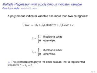
![EXERCISE: MULTIPLE REGRESSION WITH A
POLYTOMOUS INDICATOR VARIABLE
[MBA data from Keller xm18-00.sav]
20 / 24](https://image.slidesharecdn.com/business-statistics-ii-aarhus-bss-170814111356/85/Business-statistics-ii-aarhus-bss-181-320.jpg)