Educational Statistics with Software Application

1. EDUCATIONAL
STATISTICS WITH
SOFTWARE
APPLICATION
REPORTER: MARIETTA A. PAJE

2.  Statistics is the science
of collecting, organizing,
analyzing, and interpreting
numerical facts, which we
call data.
 It is a set of tools used
to organize and analyze
data.
 It helps us make
informed decisions by
identifying patterns, trends,
and relationships within

3. Why is Statistics
important to
Education?

4. Importance of
Statistics to
Education:
Tracking Student
Performance:
Data helps
educators
understand student
strengths and
weaknesses,
guiding curriculum
improvements and
teaching strategies.
Education Policy
& Planning:
Governments use
statistics to
allocate resources,
identify gaps, and
design policies for
better educational
access and quality.
Assessment &
Evaluation:
Standardized
tests and
academic
assessments rely
on statistical
analysis to
measure
educational
effectiveness.
Identifying
Trends &
Challenges:
Statistics highlight
issues like dropout
rates, literacy
levels, and
disparities in
access to
education,
enabling targeted
solutions.
Enhancing
Teaching Methods:
Research-backed
teaching
approaches, such as
adaptive learning
technologies,
depend on statistical
analysis to refine
methodologies.

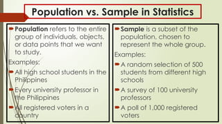
5. Population vs. Sample in Statistics
Population refers to the entire
group of individuals, objects,
or data points that we want
to study.
Examples:
All high school students in the
Philippines
Every university professor in
the Philippines
All registered voters in a
country
Sample is a subset of the
population, chosen to
represent the whole group.
Examples:
A random selection of 500
students from different high
schools
A survey of 100 university
professors
A poll of 1,000 registered
voters

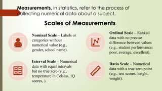
6. Measurements, in statistics, refer to the process of
collecting numerical data about a subject.
Scales of Measurements
Nominal Scale – Labels or
categories without
numerical value (e.g.,
gender, school name).
Ordinal Scale – Ranked
data with no precise
difference between values
(e.g., student performance:
poor, average, excellent).
Interval Scale – Numerical
data with equal intervals
but no true zero (e.g.,
temperature in Celsius, IQ
scores, ).
Ratio Scale – Numerical
data with a true zero point
(e.g., test scores, height,
weight).

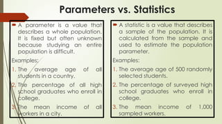
7. Parameters vs. Statistics
 A parameter is a value that
describes a whole population.
It is fixed but often unknown
because studying an entire
population is difficult.
Examples:
1. The average age of all
students in a country.
2. The percentage of all high
school graduates who enroll in
college.
3. The mean income of all
workers in a city.
 A statistic is a value that describes
a sample of the population. It is
calculated from the sample and
used to estimate the population
parameter.
Examples:
1. The average age of 500 randomly
selected students.
2. The percentage of surveyed high
school graduates who enroll in
college.
3. The mean income of 1,000
sampled workers.

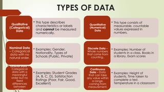
8. TYPES OF DATA
• This type describes
characteristics or labels
and cannot be measured
numerically.
Qualitative
(Categorical)
Data
• Examples: Gender,
Nationality, Types of
Schools (Public, Private)
Nominal Data
– Categorical
data with no
natural order.
• Examples: Student Grades
(A, B, C, D), Satisfaction
Ratings (Poor, Fair, Good,
Excellent)
Ordinal Data –
Categorical
data with a
meaningful
order but no
fixed
differences
between
values.
• This type consists of
measurable, countable
values expressed in
numbers.
Quantitative
(Numerical)
Data
• Examples: Number of
students in a class, Books in
a library, Exam scores
Discrete Data –
Whole numbers
that come from
counting..
• Examples: Height of
students, Time taken to
complete a test,
Temperature in a classroom
Continuous
Data – Data
that can take
any value within
a range,
coming from
measurement.

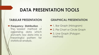
9. DATA PRESENTATION TOOLS
 Frequency Distribution -
The easiest method of
organizing data which
converts raw data into a
meaningful pattern for
statistical analysis.
GRAPHICAL PRESENTATION
 1. Bar Graph (Histogram)
 2. Pie Chart or Circle Graph
 3. Line Graph (Polygon
Method)
TABULAR PRESENTATION

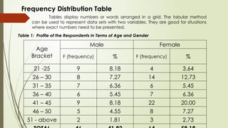
10. Frequency Distribution Table
Tables display numbers or words arranged in a grid. The tabular method
can be used to represent data sets with two variables. They are good for situations
where exact numbers need to be presented.
Table 1: Profile of the Respondents in Terms of Age and Gender
Age
Bracket
Male Female
F (frequency) % F (frequency) %
21 -25 9 8.18 4 3.64
26 – 30 8 7.27 14 12.73
31 – 35 7 6.36 6 5.45
36 – 40 6 5.45 7 6.36
41 – 45 9 8.18 22 20.00
46 – 50 5 4.55 8 7.27
51 - above 2 1.81 3 2.73

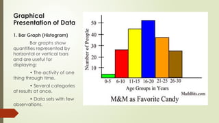
11. Graphical
Presentation of Data
1. Bar Graph (Histogram)
Bar graphs show
quantities represented by
horizontal or vertical bars
and are useful for
displaying:
• The activity of one
thing through time.
• Several categories
of results at once.
• Data sets with few
observations.

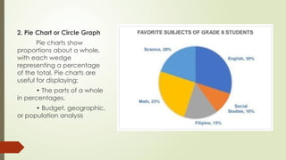
12. 2. Pie Chart or Circle Graph
Pie charts show
proportions about a whole,
with each wedge
representing a percentage
of the total. Pie charts are
useful for displaying:
• The parts of a whole
in percentages.
• Budget, geographic,
or population analysis

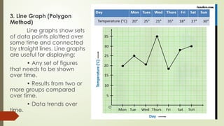
13. 3. Line Graph (Polygon
Method)
Line graphs show sets
of data points plotted over
some time and connected
by straight lines. Line graphs
are useful for displaying:
• Any set of figures
that needs to be shown
over time.
• Results from two or
more groups compared
over time.
• Data trends over
time.

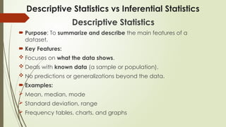
14. Descriptive Statistics vs Inferential Statistics
Descriptive Statistics
 Purpose: To summarize and describe the main features of a
dataset.
 Key Features:
 Focuses on what the data shows.
 Deals with known data (a sample or population).
 No predictions or generalizations beyond the data.
 Examples:
 Mean, median, mode
 Standard deviation, range
 Frequency tables, charts, and graphs

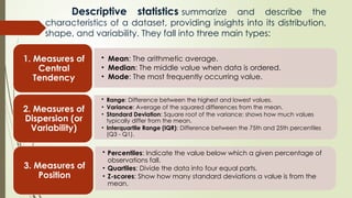
15. Descriptive statistics summarize and describe the
characteristics of a dataset, providing insights into its distribution,
shape, and variability. They fall into three main types:
• Mean: The arithmetic average.
• Median: The middle value when data is ordered.
• Mode: The most frequently occurring value.
1. Measures of
Central
Tendency
• Range: Difference between the highest and lowest values.
• Variance: Average of the squared differences from the mean.
• Standard Deviation: Square root of the variance; shows how much values
typically differ from the mean.
• Interquartile Range (IQR): Difference between the 75th and 25th percentiles
(Q3 - Q1).
2. Measures of
Dispersion (or
Variability)
• Percentiles: Indicate the value below which a given percentage of
observations fall.
• Quartiles: Divide the data into four equal parts.
• Z-scores: Show how many standard deviations a value is from the
mean.
3. Measures of
Position

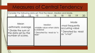
16. Measures of Central Tendency
Mean
-arithmetic average
* Divide the sum of
the data set by the
number of scores.
Median
-middle value when data
is ordered
* Denoted by read as “x
tilde”
Mode
-most frequently
occurring value
* Denoted by read
as “x hat”
Consider the following data set: Find the Mean, Median and Mode.
8 12 15 15 16 18 18 18 19 20

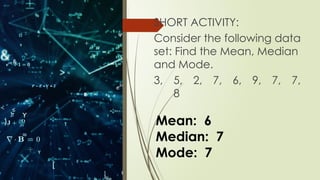
17. SHORT ACTIVITY:
Consider the following data
set: Find the Mean, Median
and Mode.
3, 5, 2, 7, 6, 9, 7, 7,
8
Mean: 6
Median: 7
Mode: 7

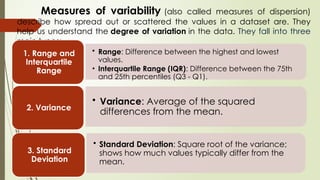
18. Measures of variability (also called measures of dispersion)
describe how spread out or scattered the values in a dataset are. They
help us understand the degree of variation in the data. They fall into three
main types:
• Range: Difference between the highest and lowest
values.
• Interquartile Range (IQR): Difference between the 75th
and 25th percentiles (Q3 - Q1).
1. Range and
Interquartile
Range
• Variance: Average of the squared
differences from the mean.
2. Variance
• Standard Deviation: Square root of the variance;
shows how much values typically differ from the
mean.
3. Standard
Deviation

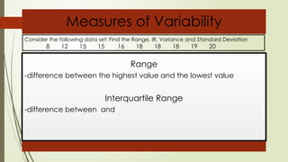
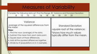
19. Measures of Variability
Range
-difference between the highest value and the lowest value
Interquartile Range
-difference between and
Consider the following data set: Find the Range, IR, Variance and Standard Deviation
8 12 15 15 16 18 18 18 19 20

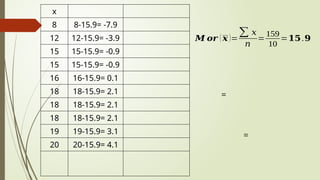
20. Measures of Variability
Variance
-average of the squared differences from
the mean
Steps:
1. Find the mean (average) of the data.
2. Subtract the mean from each data point.
3. Square each of those differences.
4. Add all the squared differences together.
5. Divide by N (population) or (n-1) (sample).
Standard Deviation
-square root of the variance;
*shows how much values
typically differ from the mean.
Consider the following data set: Find the Range, IR, Variance and Standard Deviation
8 12 15 15 16 18 18 18 19 20

21. x
8 8-15.9= -7.9
12 12-15.9= -3.9
15 15-15.9= -0.9
15 15-15.9= -0.9
16 16-15.9= 0.1
18 18-15.9= 2.1
18 18-15.9= 2.1
18 18-15.9= 2.1
19 19-15.9= 3.1
20 20-15.9= 4.1
𝑴 𝒐𝒓 ( 𝒙 )=
∑ 𝑥
𝑛
=
159
10
=𝟏𝟓.𝟗
=
=

22. Importance
of
Descriptive
Statistics
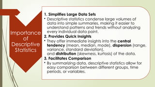
1. Simplifies Large Data Sets
• Descriptive statistics condense large volumes of
data into simple summaries, making it easier to
understand patterns and trends without analyzing
every individual data point.
2. Provides Quick Insights
• They offer immediate insights into the central
tendency (mean, median, mode), dispersion (range,
variance, standard deviation),
and distribution (skewness, kurtosis) of the data.
3. Facilitates Comparison
• By summarizing data, descriptive statistics allow for
easy comparison between different groups, time
periods, or variables.

23. Importance
of
Descriptive
Statistics
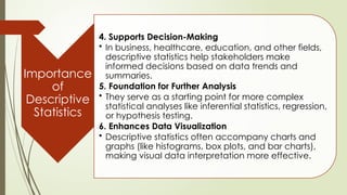
4. Supports Decision-Making
• In business, healthcare, education, and other fields,
descriptive statistics help stakeholders make
informed decisions based on data trends and
summaries.
5. Foundation for Further Analysis
• They serve as a starting point for more complex
statistical analyses like inferential statistics, regression,
or hypothesis testing.
6. Enhances Data Visualization
• Descriptive statistics often accompany charts and
graphs (like histograms, box plots, and bar charts),
making visual data interpretation more effective.

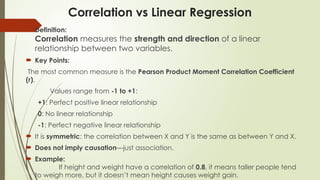
24. Correlation vs Linear Regression
 Definition:
Correlation measures the strength and direction of a linear
relationship between two variables.
 Key Points:
The most common measure is the Pearson Product Moment Correlation Coefficient
(r).
Values range from -1 to +1:
+1: Perfect positive linear relationship
0: No linear relationship
-1: Perfect negative linear relationship
 It is symmetric: the correlation between X and Y is the same as between Y and X.
 Does not imply causation—just association.
 Example:
If height and weight have a correlation of 0.8, it means taller people tend
to weigh more, but it doesn’t mean height causes weight gain.

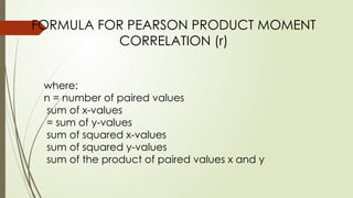
25. FORMULA FOR PEARSON PRODUCT MOMENT
CORRELATION (r)
where:
n = number of paired values
sum of x-values
= sum of y-values
sum of squared x-values
sum of squared y-values
sum of the product of paired values x and y

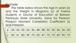
26. Example:
The table below shows the Age in years (x)
and the Weight in kilograms (y) of twelve
students in Doctor of Education at Bataan
Peninsula State University. Solve for Pearson
Product Moment Correlation Coefficient (r)
and interpret.
x 34 55 33 26 36 48 38 32 30 36 36 35
y 50 51 83 59 70 53 47 75 75 69 90 72

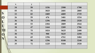
27. S
O
L
U
TI
O
N
x y
34 50 1156 2500 1700
55 51 3025 2601 2805
33 83 1089 6889 2739
26 59 676 3481 1534
36 70 1296 4900 2520
48 53 2304 2809 2544
38 47 1444 2209 1786
32 75 1024 5625 2400
30 75 900 5625 2250
36 69 1296 4761 2484
36 90 1296 8100 3240
35 72 1225 5184 2520

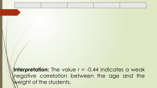
28. Interpretation: The value r = -0.44 indicates a weak
negative correlation between the age and the
weight of the students.

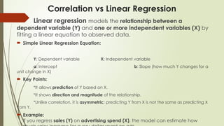
29. Correlation vs Linear Regression
Linear regression models the relationship between a
dependent variable (Y) and one or more independent variables (X) by
fitting a linear equation to observed data.
 Simple Linear Regression Equation:
Y: Dependent variable X: Independent variable
a: Intercept b: Slope (how much Y changes for a
unit change in X)
 Key Points:
*It allows prediction of Y based on X.
*It shows direction and magnitude of the relationship.
*Unlike correlation, it is asymmetric: predicting Y from X is not the same as predicting X
from Y.
 Example:
If you regress sales (Y) on advertising spend (X), the model can estimate how

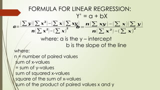
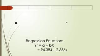
30. FORMULA FOR LINEAR REGRESSION:
Y’ = a + bX
𝒂=
(∑ 𝒚 )(∑ 𝒙𝟐
)−(∑ 𝒙)(∑ 𝒙𝒚 )
𝒏(∑ 𝒙
𝟐
)−(∑ 𝒙)
𝟐 𝒃=
𝒏(∑ 𝒙𝒚 )−(∑ 𝒙 )(∑ 𝒚 )
𝒏(∑ 𝒙𝟐
)−(∑ 𝒙)
𝟐
where: a is the y – intercept
b is the slope of the line
where:
n = number of paired values
sum of x-values
= sum of y-values
sum of squared x-values
square of the sum of x-values
sum of the product of paired values x and y

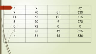
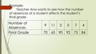
31. Example:
Teacher Ana wants to see how the number
of absences of a student affects the student’s
final grade.
Number of
Absences
9 11 3 0 7 4
Final Grade 70 65 90 92 75 84

32. x y xy
9 70 81 630
11 65 121 715
3 90 9 270
0 92 0 0
7 75 49 525
4 84 16 336

33. = =
Regression Equation:
Y’ = a + bX
= 94.384 – 2.656x

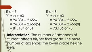
34. If x = 5
Y’ = a + bX
= 94.384 – 2.656x
= 94.384 – 2.656(5)
= 81. 104 or 81
If x = 8
Y’ = a + bX
= 94.384 – 2.656x
= 94.384 – 2.656(8)
= 73.136 or 73
Interpretation: The number of absences of
student affects his/her final grade. The more
number of absences the lower grade he/she
gets.

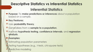
35. Descriptive Statistics vs Inferential Statistics
Inferential Statistics
 Purpose: To make predictions or inferences about a population
based on a sample.
 Key Features:
 Uses probability theory.
 Generalizes from a sample to a population.
 Involves hypothesis testing, confidence intervals, and regression
analysis.
 Examples:
 Estimating population parameters
 Testing hypotheses (e.g., t-tests, chi-square tests)
 Predictive modeling

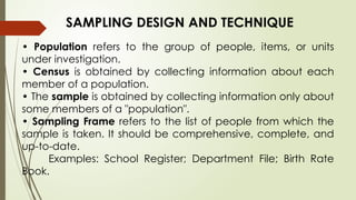
36. SAMPLING DESIGN AND TECHNIQUE
• Population refers to the group of people, items, or units
under investigation.
• Census is obtained by collecting information about each
member of a population.
• The sample is obtained by collecting information only about
some members of a "population".
• Sampling Frame refers to the list of people from which the
sample is taken. It should be comprehensive, complete, and
up-to-date.
Examples: School Register; Department File; Birth Rate
Book.

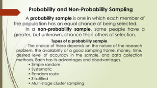
37. Probability and Non-Probability Sampling
A probability sample is one in which each member of
the population has an equal chance of being selected.
In a non-probability sample, some people have a
greater, but unknown, chance than others of selection.
Types of a probability sample
The choice of these depends on the nature of the research
problem, the availability of a good sampling frame, money, time,
desired level of accuracy in the sample, and data collection
methods. Each has its advantages and disadvantages.
• Simple random
• Systematic
• Random route
• Stratified
• Multi-stage cluster sampling

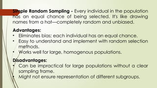
38. Simple Random Sampling - Every individual in the population
has an equal chance of being selected. It's like drawing
names from a hat—completely random and unbiased.
Advantages:
• Eliminates bias; each individual has an equal chance.
• Easy to understand and implement with random selection
methods.
• Works well for large, homogenous populations.
Disadvantages:
• Can be impractical for large populations without a clear
sampling frame.
• Might not ensure representation of different subgroups.

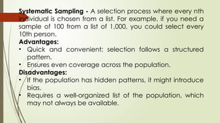
39. Systematic Sampling - A selection process where every nth
individual is chosen from a list. For example, if you need a
sample of 100 from a list of 1,000, you could select every
10th person.
Advantages:
• Quick and convenient; selection follows a structured
pattern.
• Ensures even coverage across the population.
Disadvantages:
• If the population has hidden patterns, it might introduce
bias.
• Requires a well-organized list of the population, which
may not always be available.

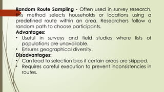
40. Random Route Sampling - Often used in survey research,
this method selects households or locations using a
predefined route within an area. Researchers follow a
random path to choose participants.
Advantages:
• Useful in surveys and field studies where lists of
populations are unavailable.
• Ensures geographical diversity.
Disadvantages:
• Can lead to selection bias if certain areas are skipped.
• Requires careful execution to prevent inconsistencies in
routes.

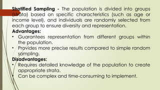
41. Stratified Sampling - The population is divided into groups
(strata) based on specific characteristics (such as age or
income level), and individuals are randomly selected from
each group to ensure diversity and representation.
Advantages:
• Guarantees representation from different groups within
the population.
• Provides more precise results compared to simple random
sampling.
Disadvantages:
• Requires detailed knowledge of the population to create
appropriate strata.
• Can be complex and time-consuming to implement.

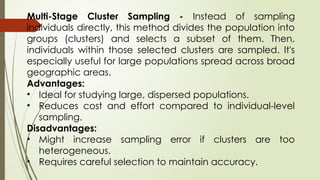
42. Multi-Stage Cluster Sampling - Instead of sampling
individuals directly, this method divides the population into
groups (clusters) and selects a subset of them. Then,
individuals within those selected clusters are sampled. It's
especially useful for large populations spread across broad
geographic areas.
Advantages:
• Ideal for studying large, dispersed populations.
• Reduces cost and effort compared to individual-level
sampling.
Disadvantages:
• Might increase sampling error if clusters are too
heterogeneous.
• Requires careful selection to maintain accuracy.

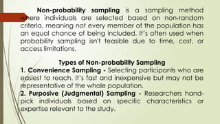
43. Non-probability sampling is a sampling method
where individuals are selected based on non-random
criteria, meaning not every member of the population has
an equal chance of being included. It’s often used when
probability sampling isn't feasible due to time, cost, or
access limitations.
Types of Non-probability Sampling
1. Convenience Sampling - Selecting participants who are
easiest to reach. It’s fast and inexpensive but may not be
representative of the whole population.
2. Purposive (Judgmental) Sampling - Researchers hand-
pick individuals based on specific characteristics or
expertise relevant to the study.

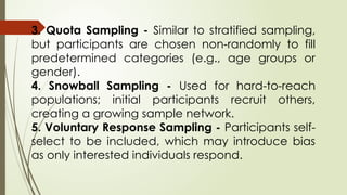
44. 3. Quota Sampling - Similar to stratified sampling,
but participants are chosen non-randomly to fill
predetermined categories (e.g., age groups or
gender).
4. Snowball Sampling - Used for hard-to-reach
populations; initial participants recruit others,
creating a growing sample network.
5. Voluntary Response Sampling - Participants self-
select to be included, which may introduce bias
as only interested individuals respond.

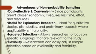
45. Advantages of Non-probability Sampling
•Cost-effective & Convenient – Since participants
aren’t chosen randomly, it requires less time, effort,
and resources.
•Useful for Exploratory Research – Ideal for qualitative
studies, pilot studies, and preliminary research where
applicability isn’t a priority.
•Targeted Selection – Allows researchers to focus on
specific subgroups that are relevant to the study.
•Flexibility – Researchers can easily adjust sample
selection based on availability and feasibility.

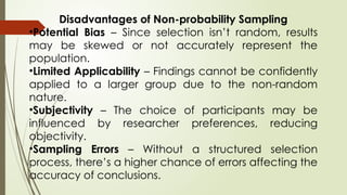
46. Disadvantages of Non-probability Sampling
•Potential Bias – Since selection isn’t random, results
may be skewed or not accurately represent the
population.
•Limited Applicability – Findings cannot be confidently
applied to a larger group due to the non-random
nature.
•Subjectivity – The choice of participants may be
influenced by researcher preferences, reducing
objectivity.
•Sampling Errors – Without a structured selection
process, there’s a higher chance of errors affecting the
accuracy of conclusions.

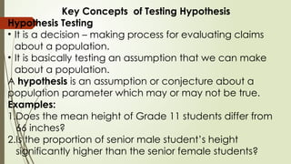
47. Key Concepts of Testing Hypothesis
Hypothesis Testing
• It is a decision – making process for evaluating claims
about a population.
• It is basically testing an assumption that we can make
about a population.
A hypothesis is an assumption or conjecture about a
population parameter which may or may not be true.
Examples:
1.Does the mean height of Grade 11 students differ from
66 inches?
2.Is the proportion of senior male student’s height
significantly higher than the senior female students?

48. The Null and Alternative Hypothesis
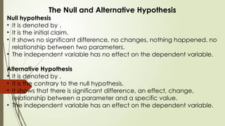
Null hypothesis
• It is denoted by .
• It is the initial claim.
• It shows no significant difference, no changes, nothing happened, no
relationship between two parameters.
• The independent variable has no effect on the dependent variable.
Alternative Hypothesis
• It is denoted by .
• It is the contrary to the null hypothesis.
• It shows that there is significant difference, an effect, change,
relationship between a parameter and a specific value.
• The independent variable has an effect on the dependent variable.

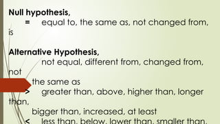
49. Null hypothesis,
= equal to, the same as, not changed from,
is
Alternative Hypothesis,
not equal, different from, changed from,
not
the same as
> greater than, above, higher than, longer
than,
bigger than, increased, at least

50. Estimation of a One-Sample Mean
It is a statistical technique used to infer
the population mean based on a sample.
Since we rarely have access to entire
populations, we use sample data to
estimate characteristics with some level of
confidence.

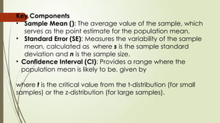
51. Key Components
• Sample Mean (): The average value of the sample, which
serves as the point estimate for the population mean.
• Standard Error (SE): Measures the variability of the sample
mean, calculated as where s is the sample standard
deviation and n is the sample size.
• Confidence Interval (CI): Provides a range where the
population mean is likely to be, given by
where t is the critical value from the t-distribution (for small
samples) or the z-distribution (for large samples).

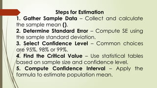
52. Steps for Estimation
1. Gather Sample Data – Collect and calculate
the sample mean ().
2. Determine Standard Error – Compute SE using
the sample standard deviation.
3. Select Confidence Level – Common choices
are 95%, 98% or 99%.
4. Find the Critical Value – Use statistical tables
based on sample size and confidence level.
5. Compute Confidence Interval – Apply the
formula to estimate population mean.

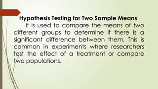
53. Hypothesis Testing for Two Sample Means
It is used to compare the means of two
different groups to determine if there is a
significant difference between them. This is
common in experiments where researchers
test the effect of a treatment or compare
two populations.

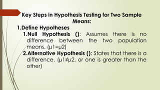
54. Key Steps in Hypothesis Testing for Two Sample
Means:
1.Define Hypotheses
1.Null Hypothesis (): Assumes there is no
difference between the two population
means. (μ1=μ2)
2.Alternative Hypothesis (): States that there is a
difference. (μ1≠μ2, or one is greater than the
other)

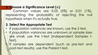
55. 2. Choose a Significance Level ( )
𝛼
Common values are 0.05 (5%) or 0.01 (1%),
representing the probability of rejecting the null
hypothesis when it's actually true.
3. Select the Appropriate Test
• If population variances are known, use the Z-test.
• If population variances are unknown or sample sizes
are small, use the t-test (Independent Samples t-
test).
• If samples are dependent (such as pre-test and
post-test results), use the Paired t-test.

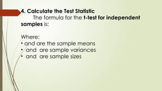
56. 4. Calculate the Test Statistic
The formula for the t-test for independent
samples is:
Where:
• and are the sample means
• and are sample variances
• and are sample sizes

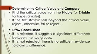
57. 5. Determine the Critical Value and Compare
• Find the critical value from the t-table (or Z-table
for large samples).
• If the test statistic falls beyond the critical value,
reject , otherwise, fail to reject .
6. Draw Conclusions
• If is rejected, it suggests a significant difference
between the two groups.
• If is not rejected, there is no sufficient evidence
to claim a difference.

58. Power and Sample Size are crucial aspects of
statistical analysis, especially in hypothesis testing.
They help determine the reliability and validity of a
study.
Statistical Power
•Power refers to the probability of correctly rejecting
a false null hypothesis ().
•A study with high power means it can detect an
effect when one truly exists.

59. Power is influenced by:
• Sample size – Larger samples provide more
accurate estimates.
• Effect size – Larger differences are easier to
detect.
• Significance level () – Typically set at 0.05.
• Variance – Lower variability improves
detection of effects.

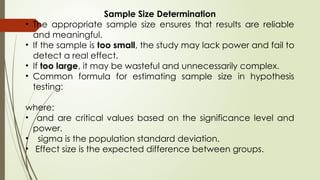
60. Sample Size Determination
• The appropriate sample size ensures that results are reliable
and meaningful.
• If the sample is too small, the study may lack power and fail to
detect a real effect.
• If too large, it may be wasteful and unnecessarily complex.
• Common formula for estimating sample size in hypothesis
testing:
where:
• and are critical values based on the significance level and
power.
• sigma is the population standard deviation.
• Effect size is the expected difference between groups.

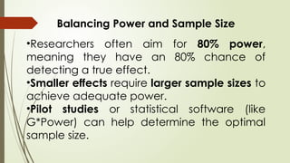
61. Balancing Power and Sample Size
•Researchers often aim for 80% power,
meaning they have an 80% chance of
detecting a true effect.
•Smaller effects require larger sample sizes to
achieve adequate power.
•Pilot studies or statistical software (like
G*Power) can help determine the optimal
sample size.

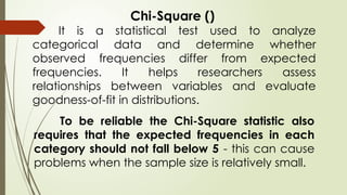
62. Chi-Square ()
It is a statistical test used to analyze
categorical data and determine whether
observed frequencies differ from expected
frequencies. It helps researchers assess
relationships between variables and evaluate
goodness-of-fit in distributions.
To be reliable the Chi-Square statistic also
requires that the expected frequencies in each
category should not fall below 5 - this can cause
problems when the sample size is relatively small.

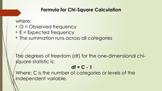
63. The degrees of freedom (df) for the one-dimensional chi-
square statistic is:
df = C - 1
Where: C is the number of categories or levels of the
independent variable.
Formula for Chi-Square Calculation
where:
• O = Observed frequency
• E = Expected frequency
• The summation runs across all categories

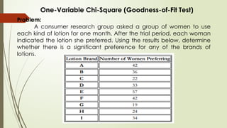
64. One-Variable Chi-Square (Goodness-of-Fit Test)
Problem:
A consumer research group asked a group of women to use
each kind of lotion for one month. After the trial period, each woman
indicated the lotion she preferred. Using the results below, determine
whether there is a significant preference for any of the brands of
lotions.

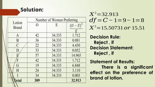
65. Lotion
Brand
Number of Women Preferring
O E
A 42 34.333 1.712
B 36 34.333 0.081
C 22 34.333 4.430
D 33 34.333 0.052
E 57 34.333 14.965
F 42 34.333 1.712
G 19 34.333 6.848
H 24 34.333 3.110
I 34 34.333 0.003
Total 309 32.913
Solution:
𝑋2
=32.913
𝑑𝑓 =𝐶− 1=9− 1=8
𝑋2
=15.50731 𝑜𝑟 15.51
Decision Rule:
Reject , if
Decision Statement:
Reject , if
Statement of Results:
There is a significant
effect on the preference of
brand of lotion.

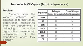
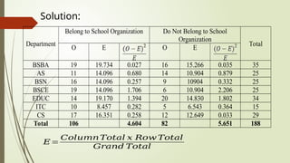
67. Two-Variable Chi-Square (Test of Independence)
Problem:
Students from the
various colleges are
classified as to their school
organization membership
and their department. Is
belonging to a school
organization membership
independent of the
department where they
belong?

68. Department
Belong to School Organization Do Not Belong to School
Organization
Total
O E O E
BSBA 19 19.734 0.027 16 15.266 0.035 35
AS 11 14.096 0.680 14 10.904 0.879 25
BSN 16 14.096 0.257 9 10904 0.332 25
BSCE 19 14.096 1.706 6 10.904 2.206 25
EDUC 14 19.170 1.394 20 14.830 1.802 34
ITC 10 8.457 0.282 5 6.543 0.364 15
CS 17 16.351 0.258 12 12.649 0.033 29
Total 106 4.604 82 5.651 188
Solution:
𝐸=
𝐶𝑜𝑙𝑢𝑚𝑛𝑇𝑜𝑡𝑎𝑙 𝑥 𝑅𝑜𝑤 𝑇𝑜𝑡𝑎𝑙
𝐺𝑟𝑎𝑛𝑑 𝑇𝑜𝑡𝑎𝑙

69. Alpha Level:
Calculated Value:

70. Decision Rule:
Reject , if
Decision Statement:
Fail to reject .
Statement of Results:
There is no significant relationship
between belonging and not belonging to
a school organization among college
students in every department.

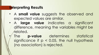
71. Interpreting Results
• A small value suggests the observed and
expected values are similar.
• A large value indicates a significant
difference, meaning the variables might be
related.
• The p-value determines statistical
significance if p < 0.05, the null hypothesis
(no association) is rejected.

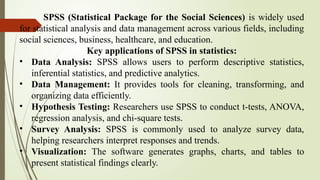
72. SPSS (Statistical Package for the Social Sciences) is widely used
for statistical analysis and data management across various fields, including
social sciences, business, healthcare, and education.
Key applications of SPSS in statistics:
• Data Analysis: SPSS allows users to perform descriptive statistics,
inferential statistics, and predictive analytics.
• Data Management: It provides tools for cleaning, transforming, and
organizing data efficiently.
• Hypothesis Testing: Researchers use SPSS to conduct t-tests, ANOVA,
regression analysis, and chi-square tests.
• Survey Analysis: SPSS is commonly used to analyze survey data,
helping researchers interpret responses and trends.
• Visualization: The software generates graphs, charts, and tables to
present statistical findings clearly.