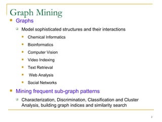
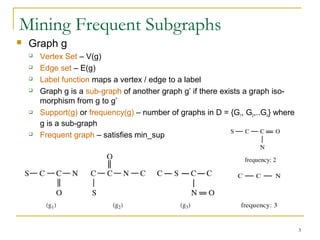
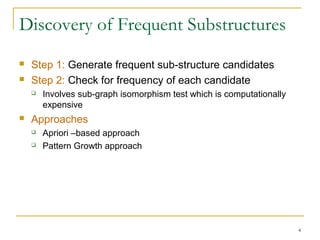
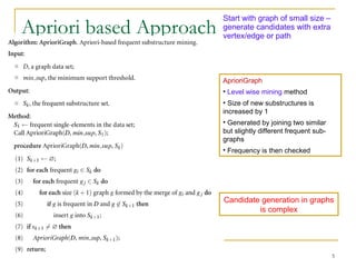
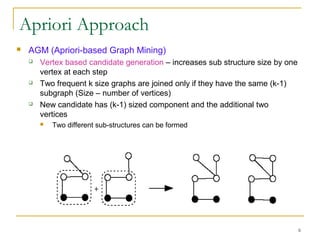
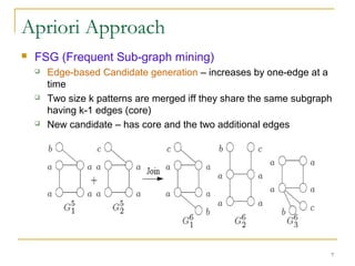
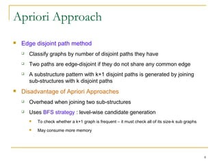
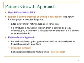
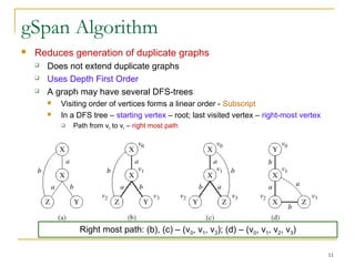
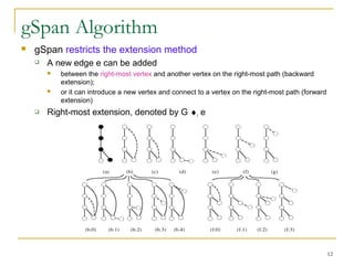
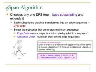
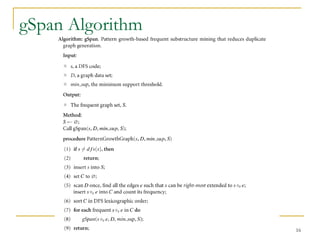
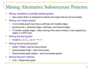
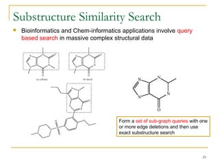
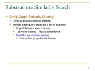
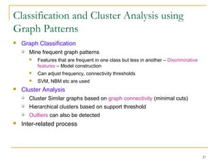
Graph mining involves discovering frequent subgraphs, patterns, or substructures from a graph database. It has applications in domains like cheminformatics, bioinformatics, social network analysis, and knowledge discovery. There are two main approaches for frequent subgraph mining - Apriori-based approaches that generate candidates level-wise and pattern growth approaches that extend frequent subgraphs. The gSpan algorithm reduces redundant searching by using a depth-first search ordering of the graphs. Mining closed, maximal or dense frequent subgraphs can further reduce the number of patterns discovered. Applications include graph indexing, substructure similarity search, and graph classification or clustering.

1. Graph Mining
1

2. Graph Mining
 Graphs
 Model sophisticated structures and their interactions
 Chemical Informatics
 Bioinformatics
 Computer Vision
 Video Indexing
 Text Retrieval
 Web Analysis
 Social Networks
 Mining frequent sub-graph patterns
 Characterization, Discrimination, Classification and Cluster
Analysis, building graph indices and similarity search
2

3. Mining Frequent Subgraphs
 Graph g
 Vertex Set – V(g)
 Edge set – E(g)
 Label function maps a vertex / edge to a label
 Graph g is a sub-graph of another graph g’ if there exists a graph iso-
morphism from g to g’
 Support(g) or frequency(g) – number of graphs in D = {G1, G2,..Gn} where
g is a sub-graph
 Frequent graph – satisfies min_sup
3

4. Discovery of Frequent Substructures
 Step 1: Generate frequent sub-structure candidates
 Step 2: Check for frequency of each candidate
 Involves sub-graph isomorphism test which is computationally
expensive
 Approaches
 Apriori –based approach
 Pattern Growth approach
4

5. Apriori based Approach
5
Start with graph of small size –
generate candidates with extra
vertex/edge or path
AprioriGraph
• Level wise mining method
• Size of new substructures is
increased by 1
• Generated by joining two similar
but slightly different frequent sub-
graphs
• Frequency is then checked
Candidate generation in graphs
is complex

6. Apriori Approach
 AGM (Apriori-based Graph Mining)
 Vertex based candidate generation – increases sub structure size by one
vertex at each step
 Two frequent k size graphs are joined only if they have the same (k-1)
subgraph (Size – number of vertices)
 New candidate has (k-1) sized component and the additional two
vertices
 Two different sub-structures can be formed
6

7. Apriori Approach
 FSG (Frequent Sub-graph mining)
 Edge-based Candidate generation – increases by one-edge at a
time
 Two size k patterns are merged iff they share the same subgraph
having k-1 edges (core)
 New candidate – has core and the two additional edges
7

8. Apriori Approach
 Edge disjoint path method
 Classify graphs by number of disjoint paths they have
 Two paths are edge-disjoint if they do not share any common edge
 A substructure pattern with k+1 disjoint paths is generated by joining
sub-structures with k disjoint paths
 Disadvantage of Apriori Approaches
 Overhead when joining two sub-structures
 Uses BFS strategy : level-wise candidate generation
 To check whether a k+1 graph is frequent – it must check all of its size-k sub graphs
 May consume more memory
8

9. Pattern-Growth Approach
 Uses BFS as well as DFS
 A graph g can be extended by adding a new edge e. The newly
formed graph is denoted by g ♦x e.
 Edge e may or may not introduce a new vertex to g.
 If e introduces a new vertex, the new graph is denoted by g ♦xf e,
otherwise, g ♦xb e, where f or b indicates that the extension is in a forward
or backward direction.
 Pattern Growth Approach
 For each discovered graph g performs extensions recursively until all
frequent graphs with g are found
 Simple but inefficient
 Same graph is discovered multiple times – duplicate graph
9

10. Pattern Growth
10

11. gSpan Algorithm
 Reduces generation of duplicate graphs
 Does not extend duplicate graphs
 Uses Depth First Order
 A graph may have several DFS-trees
 Visiting order of vertices forms a linear order - Subscript
 In a DFS tree – starting vertex – root; last visited vertex – right-most vertex
 Path from v0 to vn – right most path
11
Right most path: (b), (c) – (v0, v1, v3); (d) – (v0, v1, v2, v3)

12. gSpan Algorithm
 gSpan restricts the extension method
 A new edge e can be added
 between the right-most vertex and another vertex on the right-most path (backward
extension);
 or it can introduce a new vertex and connect to a vertex on the right-most path (forward
extension)
 Right-most extension, denoted by G ♦r e
12

13. gSpan Algorithm
 Chooses any one DFS tree – base subscripting and
extends it
 Each subscripted graph is transformed into an edge sequence –
DFS code
 Select the subscript that generates minimum sequence
 Edge Order – maps edges in a subscripted graph into a sequence
 Sequence Order – builds an order among edge sequences
13
Introduce backward edges:
Given a vertex v all of its backward edges should appear before
its forward edges (if any); If there are two backward edges (i,j1)
appears before (i,j2)
Order of forward edges: (0,1) (1,2) (1,3)
Complete sequence: (0,1) (1,2) (2,0) (1,3)

14. gSpan Algorithm
14
DFS Lexicographic Ordering: Edge order, First Vertex label, Edge label, Second Vertex label
Here γ0 < γ1 < γ2
γ0 – Minimum DFS Code
Corresponding subscript – Base
Subscripting
gSpan – carries out right most
extension on the minimum
DFS code
gSpan – carries out right most
extension on the minimum
DFS code

15. gSpan Algorithm
 Root – Empty code
 Each node is a DFS code encoding a graph
 Each edge – rightmost extension from a (k-1) length DFS code to a
k-length DFS code
 If codes s and s’ encode the same graph – search space s’ can be safely
pruned
15

16. gSpan Algorithm
16

17. Mining Closed Frequent Substructures
 Helps to overcome the problem of pattern explosion
 A frequent graph G is closed if and only if there is no proper super graph G0
that has the same support as G.
 Closegraph Algorithm
 A frequent pattern G is maximal if and only if there is no frequent super-
pattern of G.
 Maximal pattern set is a subset of the closed pattern set.
 But cannot be used to reconstruct entire set of frequent patterns
17

18. Mining Alternative Substructure Patterns
 Mining unlabeled or partially labeled graphs
 New empty label φ is assigned to vertices and edges that do not have labels
 Mining non-simple graphs
 A non simple graph may have a self-loop and multiple edges
 growing order - backward edges, self-loops, and forward edges
 To handle multiple edges - allow sharing of the same vertices in two neighboring
edges in a DFS code
 Mining directed graphs
 6-tuple (i; j; d; li; l(i; j) ; lj ); d = +1 / -1
 Mining disconnected graphs
 Graph / Pattern may be disconnected
 Disconnected Graph – Add virtual vertex
 Disconnected graph pattern – set of connected graphs
 Mining frequent subtrees
 Tree – Degenerate graph
18

19. Constraint based Mining of Substructure
Patterns
 Element, set, or subgraph containment constraint
 user requires that the mined patterns contain a particular set of
subgraphs - Succinct constraint
 Geometric constraint
 A geometric constraint can be that the angle between each pair of
connected edges must be within a range – Anti-monotonic constraint
 Value-sum constraint
 the sum_of (positive) weights on the edges, must be within a range low
and high – (sum > low) Monotonic / Anti-monotonic (sum < high)
 Multiple categories of constraints may also be enforced
19

20. Mining Approximate Frequent Substructures
 Approximate frequent substructures allow slight structural variations
 Several slightly different frequent substructures can be represented
using one approximate substructure
 SUBDUE – Substructure discovery system
 based on the Minimum Description Length (MDL) principle
 adopts a constrained beam search
 SUBDUE performs approximate matching
20

21. Mining Coherent and Dense Sub structures
 A frequent substructure G is a coherent sub graph if the mutual information
between G and each of its own sub graphs is above some threshold
 Reduces number of patterns mined
 Application: coherent substructure mining selects a small subset of features that have high
distinguishing power between protein classes.
 Relational graph –each label is used only once
 Frequent highly connected or dense subgraph mining
 People with strong associations in OSNs
 Set of genes within the same functional module
 Cannot judge based on average degree or minimal degree
 Must ensure connectedness
 Example: Average degree: 3.25
Minimum degree 3
21

22. Mining Dense Substructures
 Dense graphs defined in terms of Edge Connectivity
 Given a graph G, an edge cut is a set of edges Ec such that E(G) - Ec is
disconnected.
 A minimum cut is the smallest set in all edge cuts.
 The edge connectivity of G is the size of a minimum cut.
 A graph is dense if its edge connectivity is no less than a specified minimum cut
threshold
 Mining Dense substructures
 Pattern-growth approach called Close-Cut (Scalable)
 starts with a small frequent candidate graph and extends it until it finds the largest super graph with the
same support
 Pattern-reduction approach called Splat (High performance)
 directly intersects relational graphs to obtain highly connected graphs
 A pattern g discovered in a set is progressively intersected with subsequent components to give g’
 Some edges in g may be removed
 The size of candidate graphs is reduced by intersection and decomposition operations.
22

23. Applications – Graph Indexing
 Indexing is essential for efficient search and query processing
 Traditional approaches are not feasible for graphs
 Indexing based on nodes / edges / sub-graphs
 Path based Indexing approach
 Enumerate all the paths in a database up to maxL length and index them
 Index is used to identify all graphs with the paths in query
 Not suitable for complex graph queries
 Structural information is lost when a query graph is broken apart
 Many false positives maybe returned
 gIndex – considers frequent and discriminative substructures as index features
 A frequent substructure is discriminative if its support cannot be approximated by the intersection of the
graph sets
 Achieves good performance at less cost
23

24. Graph Indexing
24
Only (c) is an exact match, but
others are also reported due to the
presence of sub-structures

25. Substructure Similarity Search
 Bioinformatics and Chem-informatics applications involve query
based search in massive complex structural data
25
Form a set of sub-graph queries with one
or more edge deletions and then use
exact substructure search

26. Substructure Similarity Search
 Grafil (Graph Similarity Filtering)
 Feature based structural filtering
 Models each query graph as a set of features
 Edge deletions – feature misses
 Too many features – reduce performance
 Multi-filter composition strategy
 Feature Set - group of similar features
26

27. Classification and Cluster Analysis using
Graph Patterns
 Graph Classification
 Mine frequent graph patterns
 Features that are frequent in one class but less in another – Discriminative
features – Model construction
 Can adjust frequency, connectivity thresholds
 SVM, NBM etc are used
 Cluster Analysis
 Cluster Similar graphs based on graph connectivity (minimal cuts)
 Hierarchical clusters based on support threshold
 Outliers can also be detected
 Inter-related process
27