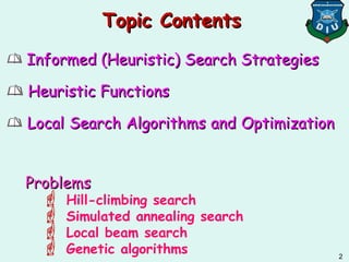
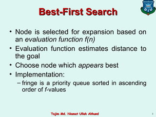
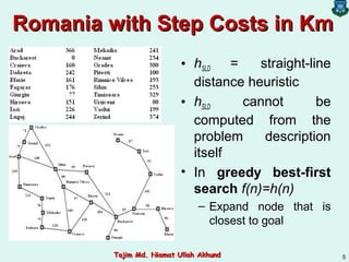
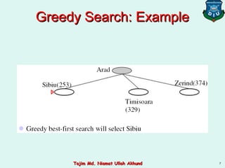
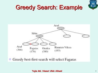
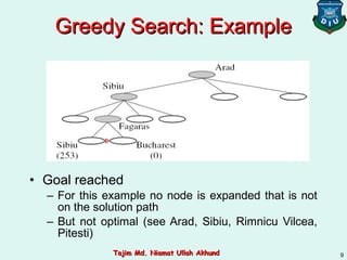
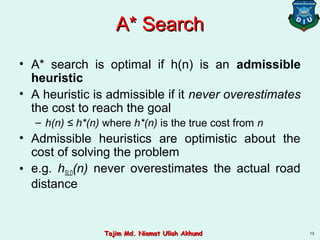
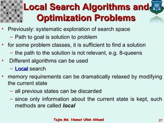
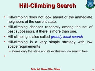
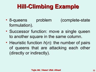
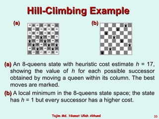
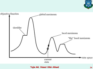
This document discusses informed search strategies and local search algorithms for optimization problems. It covers best-first search, greedy search, A* search, heuristic functions, hill-climbing search, and escaping local optima. Specifically, it provides examples of applying greedy search, A* search, and hill-climbing to solve the 8-puzzle problem and discusses the drawbacks of hill-climbing getting stuck at local maxima.


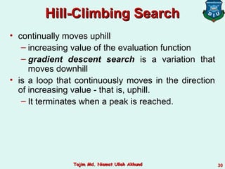

![Hill-Climbing SearchHill-Climbing Search
function HILL-CLIMBING( problem) return a state that is a local maximum
input: problem, a problem
local variables: current, a node.
neighbor, a node.
current ← MAKE-NODE(INITIAL-STATE[problem])
loop do
neighbor ← a highest valued successor of current
if VALUE [neighbor] ≤ VALUE[current] then return STATE[current]
current ← neighbor
39Tajim Md. Niamat Ullah AkhundTajim Md. Niamat Ullah Akhund](https://image.slidesharecdn.com/topic-4informedsearchandexploration-190426041240/85/AI-Lecture-4-informed-search-and-exploration-39-320.jpg)

![function SIMULATED-ANNEALING( problem, schedule) return a solution state
input: problem, a problem
schedule, a mapping from time to temperature
local variables: current, a node.
next, a node.
T, a “temperature” controlling the probability of downward steps
current ← MAKE-NODE(INITIAL-STATE[problem])
for t ← 1 to ∞ do
T ← schedule[t]
if T = 0 then return current
next ← a randomly selected successor of current
∆E ← VALUE[next] - VALUE[current]
if ∆E > 0 then current ← next
else current ← next only with probability e∆E /T
Simulated AnnealingSimulated Annealing
42Tajim Md. Niamat Ullah AkhundTajim Md. Niamat Ullah Akhund](https://image.slidesharecdn.com/topic-4informedsearchandexploration-190426041240/85/AI-Lecture-4-informed-search-and-exploration-42-320.jpg)