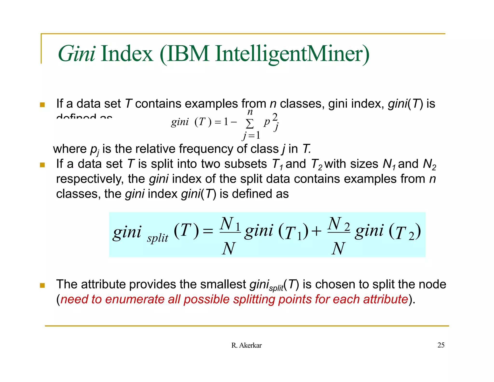
Here are the steps to construct the decision tree using the Gini index approach: 1. Calculate the Gini index for the total dataset: Gini(Total) = 1 - (19/40)2 - (21/40)2 = 0.5 2. Calculate the Gini index for age <= 50 split: Gini(S1) = 1 - (8/19)2 - (11/19)2 = 0.3789 Gini(S2) = 1 - (11/21)2 - (10/21)2 = 0.4762 3. Calculate the Gini index for the split: Gini(Split) = (19

1. Decision Tree
R. Akerkar
TMRF, Kolhapur, India
1
R. Akerkar

2. Introduction
 A classification scheme which generates a tree and
a set of rules from given data set.
 The set of records available for developing
classification methods is divided into two disjoint
subsets – a training set and a test set.
 The attributes of the records are categorise into two
types:
 Attributes whose domain is numerical are called numerical
attributes.
 Attributes whose domain is not numerical are called the
categorical attributes.
2
R. Akerkar

3. Introduction
 A decision tree is a tree with the following properties:
 An inner node represents an attribute.
 An edge represents a test on the attribute of the father
node.
 A leaf represents one of the classes.
 Construction of a decision tree
 Based on the training data
 Top-Down strategy
3
R. Akerkar

4. Decision Tree
Example
 The data set has five attributes.
 There is a special attribute: the attribute class is the class label.
 The attributes, temp (temperature) and humidity are numerical
attributes
 Other attributes are categorical, that is, they cannot be ordered.
 Based on the training data set, we want to find a set of rules to
know what values of outlook, temperature, humidity and wind,
determine whether or not to play golf.
4
R. Akerkar

5. Decision Tree
Example
 We have five leaf nodes.
 In a decision tree, each leaf node represents a rule.
 We have the following rules corresponding to the tree given in
Figure.
 RULE 1
 RULE 2
 RULE 3
 RULE 4
 RULE 5
If it is sunny and the humidity is not above 75%, then play.
If it is sunny and the humidity is above 75%, then do not play.
If it is overcast, then play.
If it is rainy and not windy, then play.
If it is rainy and windy, then don't play.
5
R. Akerkar

6. Classification
 The classification of an unknown input vector is done by
traversing the tree from the root node to a leaf node.
 A record enters the tree at the root node.
 At the root, a test is applied to determine which child
node the record will encounter next.
 This process is repeated until the record arrives at a leaf
node.
 All the records that end up at a given leaf of the tree are
classified in the same way.
 There is a unique path from the root to each leaf.
 The path is a rule which is used to classify the records.
6
R. Akerkar

7.  In our tree, we can carry out the classification
for an unknown record as follows.
 Let us assume, for the record, that we know
the values of the first four attributes (but we
do not know the value of class attribute) as
 outlook= rain; temp = 70; humidity = 65; and
windy= true.
7
R. Akerkar

8.  We start from the root node to check the value of the attribute
associated at the root node.
 This attribute is the splitting attribute at this node.
 For a decision tree, at every node there is an attribute associated
with the node called the splitting attribute.
 In our example, outlook is the splitting attribute at root.
 Since for the given record, outlook = rain, we move to the right-
most child node of the root.
 At this node, the splitting attribute is windy and we find that for
the record we want classify, windy = true.
 Hence, we move to the left child node to conclude that the class
label Is "no play".
8
R. Akerkar

9.  The accuracy of the classifier is determined by the percentage of the
test data set that is correctly classified.
 We can see that for Rule 1 there are two records of the test data set
satisfying outlook= sunny and humidity < 75, and only one of these
is correctly classified as play.
 Thus, the accuracy of this rule is 0.5 (or 50%). Similarly, the
accuracy of Rule 2 is also 0.5 (or 50%). The accuracy of Rule 3 is
0.66.
RULE 1
If it is sunny and the humidity
is not above 75%, then play.
9
R. Akerkar

10. Concept of Categorical Attributes
 Consider the following training
data set.
 There are three attributes,
namely, age, pincode and class.
 The attribute class is used for
class label.
The attribute age is a numeric attribute, whereas pincode is a categorical
one.
Though the domain of pincode is numeric, no ordering can be defined
among pincode values.
You cannot derive any useful information if one pin-code is greater than
another pincode.
10
R. Akerkar

11.  Figure gives a decision tree for the
training data.
 The splitting attribute at the root is
pincode and the splitting criterion
here is pincode = 500 046.
 Similarly, for the left child node, the
splitting criterion is age < 48 (the
splitting attribute is age).
 Although the right child node has
the same attribute as the splitting
attribute, the splitting criterion is
different.
At root level, we have 9 records.
The associated splitting criterion is
pincode = 500 046.
As a result, we split the records
into two subsets. Records 1, 2, 4, 8,
and 9 are to the left child note and
remaining to the right node.
The process is repeated at every
node.
11
R. Akerkar

12. Advantages and Shortcomings of Decision
Tree Classifications
 A decision tree construction process is concerned with identifying
the splitting attributes and splitting criterion at every level of the tree.
 Major strengths are:
 Decision tree able to generate understandable rules.
 They are able to handle both numerical and categorical attributes.
 They provide clear indication of which fields are most important for
prediction or classification.
 Weaknesses are:
 The process of growing a decision tree is computationally expensive. At
each node, each candidate splitting field is examined before its best split
can be found.
 Some decision tree can only deal with binary-valued target classes.
12
R. Akerkar

13. Iterative Dichotomizer (ID3)
 Quinlan (1986)
 Each node corresponds to a splitting attribute
 Each arc is a possible value of that attribute.
 At each node the splitting attribute is selected to be the most
informative among the attributes not yet considered in the path from
the root.
 Entropy is used to measure how informative is a node.
 The algorithm uses the criterion of information gain to determine the
goodness of a split.
 The attribute with the greatest information gain is taken as
the splitting attribute, and the data set is split for all distinct
values of the attribute.
13
R. Akerkar

14. Training Dataset
This follows an example from Quinlan’s ID3
The class label attribute,
buys_computer, has two distinct
values.
Thus there are two distinct
classes. (m =2)
Class C1 corresponds to yes
and class C2 corresponds to no.
There are 9 samples of class yes
and 5 samples of class no.
age income student credit_rating buys_computer
<=30 high no fair no
<=30 high no excellent no
31…40 high no fair yes
>40 medium no fair yes
>40 low yes fair yes
>40 low yes excellent no
31…40 low yes excellent yes
<=30 medium no fair no
<=30 low yes fair yes
>40 medium yes fair yes
<=30 medium yes excellent yes
31…40 medium no excellent yes
31…40 high yes fair yes
>4 medium n excellent n
14
R. Akerkar

15. Extracting Classification Rules from Trees
 Represent the knowledge in
the form of IF-THEN rules
 One rule is created for each
path from the root to a leaf
 Each attribute-value pair
along a path forms a
conjunction
 The leaf node holds the class
prediction
 Rules are easier for humans
to understand
What are the rules?
15
R. Akerkar

16. Solution (Rules)
IF age = “<=30” AND student = “no” THEN buys_computer = “no”
IF age = “<=30” AND student = “yes” THEN buys_computer = “yes”
IF age = “31…40” THEN buys_computer = “yes”
IF age = “>40” AND credit_rating = “excellent” THEN
buys_computer = “yes”
IF age = “<=30” AND credit_rating = “fair” THEN buys_computer =
“no”
16
R. Akerkar

17. Algorithm for Decision Tree Induction
 Basic algorithm (a greedy algorithm)
 Tree is constructed in a top-down recursive divide-and-conquer
manner
 At start, all the training examples are at the root
 Attributes are categorical (if continuous-valued, they are
discretized in advance)
 Examples are partitioned recursively based on selected attributes
 Test attributes are selected on the basis of a heuristic or
statistical measure (e.g., information gain)
 Conditions for stopping partitioning
 All samples for a given node belong to the same class
 There are no remaining attributes for further partitioning –
majority voting is employed for classifying the leaf
 There are no samples left
17
R. Akerkar

18. Attribute Selection Measure: Information
Gain (ID3/C4.5)
 Select the attribute with the highest information gain
 S contains si tuples of class Ci for i = {1, …, m}
 information measures info required to classify any
arbitrary tuple
 ….information is encoded in bits.
s s
si
log 2
si
i1
m
I( s1,s2,...,sm )  

 entropy of attribute A with values {a1,a2,…,av}
s
I(s1j,...,smj )
s1j ...smj
v
E(A)
j1
18
R. Akerkar
 information gained by branching on attribute A
Gain(A)  I(s 1,s 2,...,sm) E(A)

19. Entropy
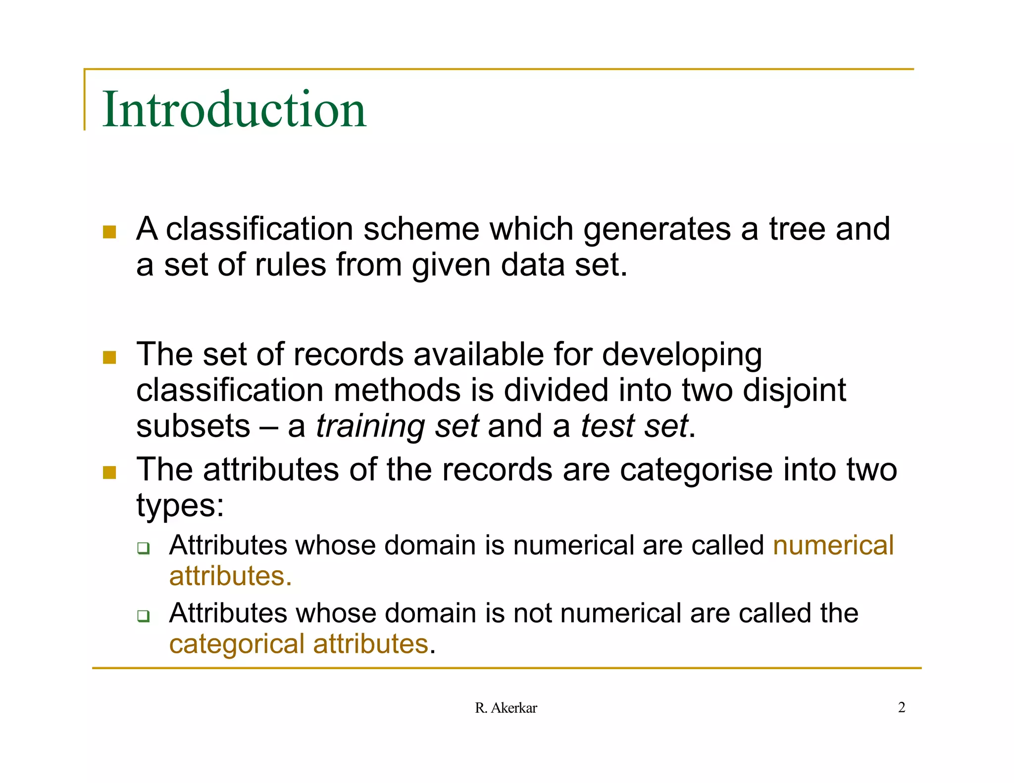
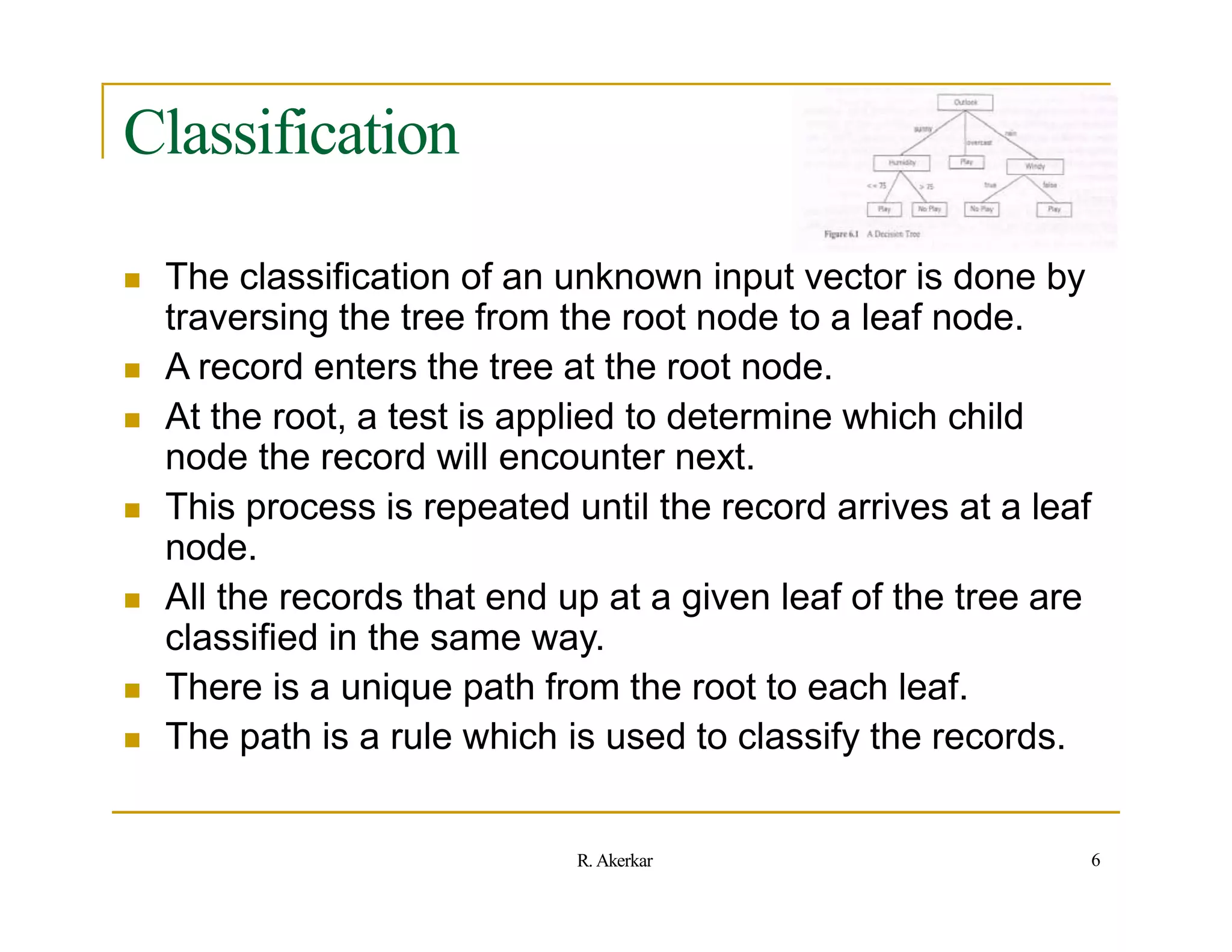
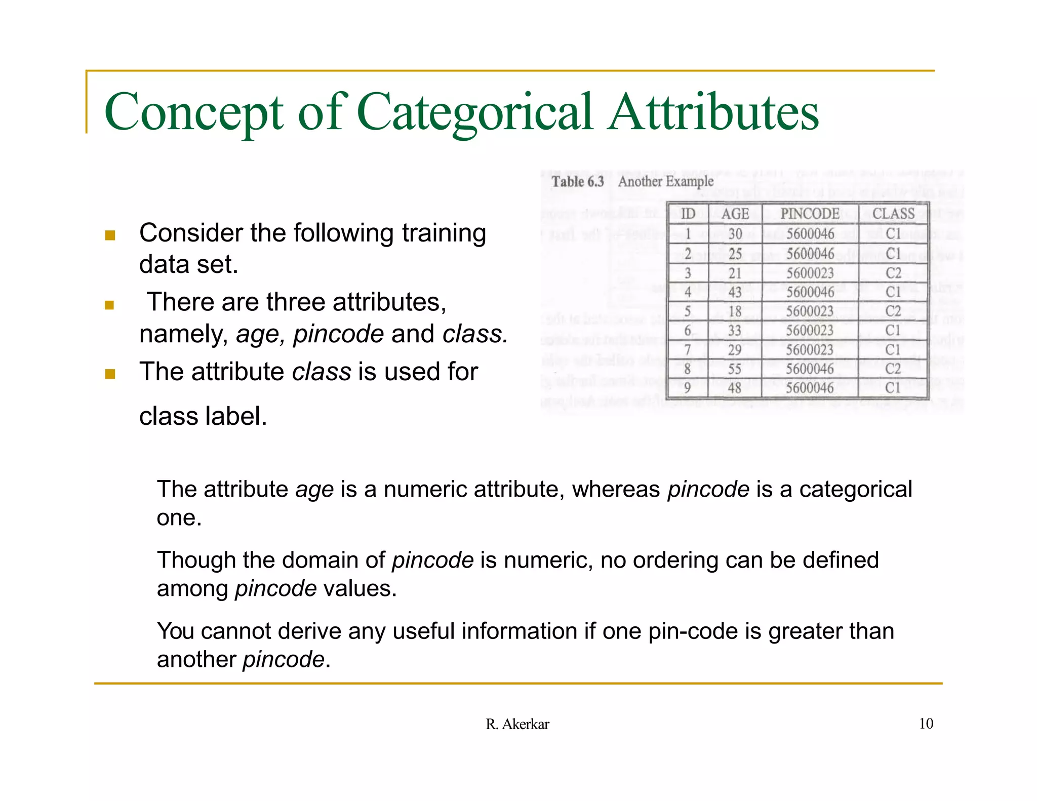
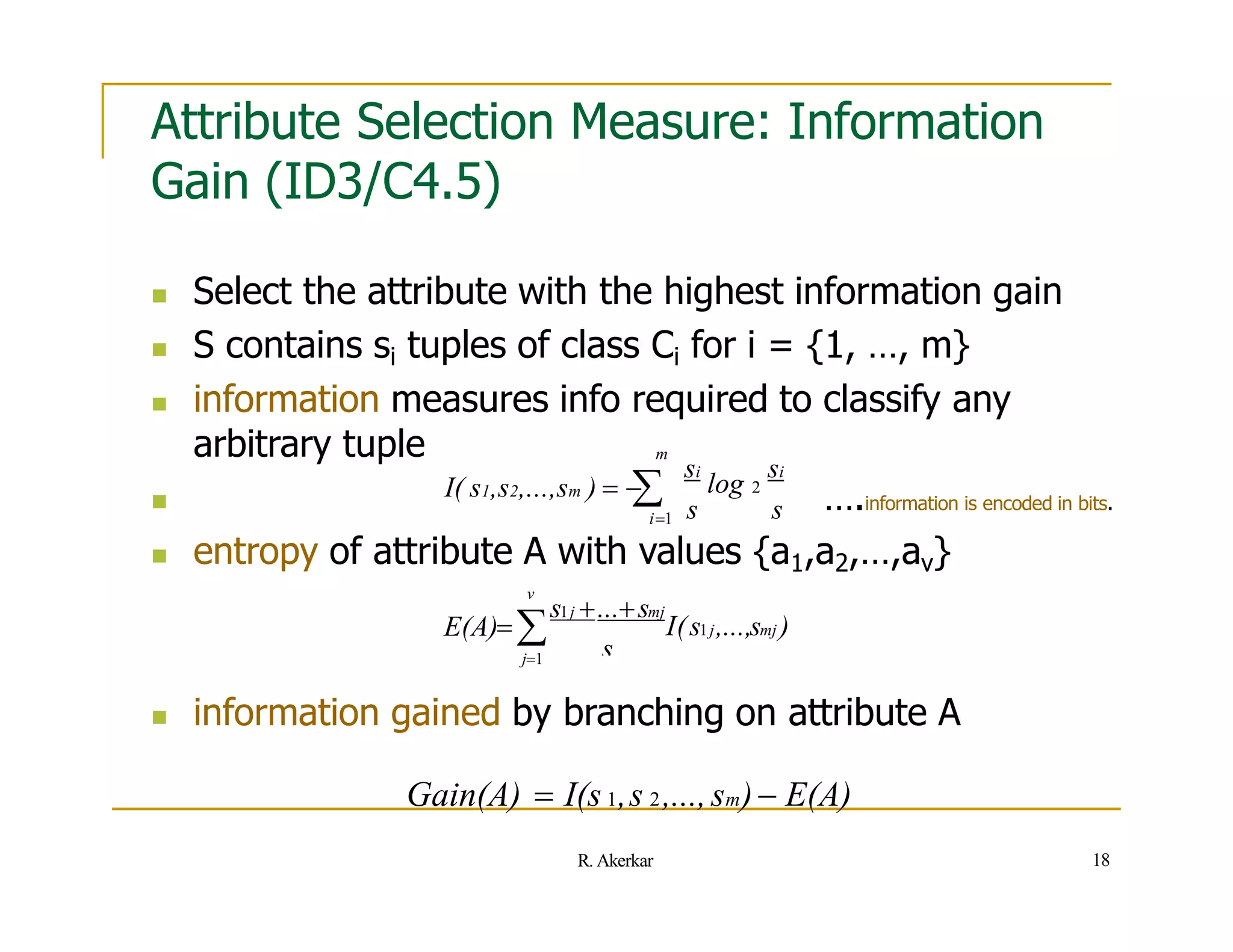
 Entropy measures the homogeneity (purity) of a set of examples.
 It gives the information content of the set in terms of the class labels of
the examples.
 Consider that you have a set of examples, S with two classes, P and N. Let
the set have p instances for the class P and n instances for the class N.
 So the total number of instances we have is t = p + n. The view [p, n] can
be seen as a class distribution of S.
The entropy for S is defined as
 Entropy(S) = - (p/t).log2(p/t) - (n/t).log2(n/t)
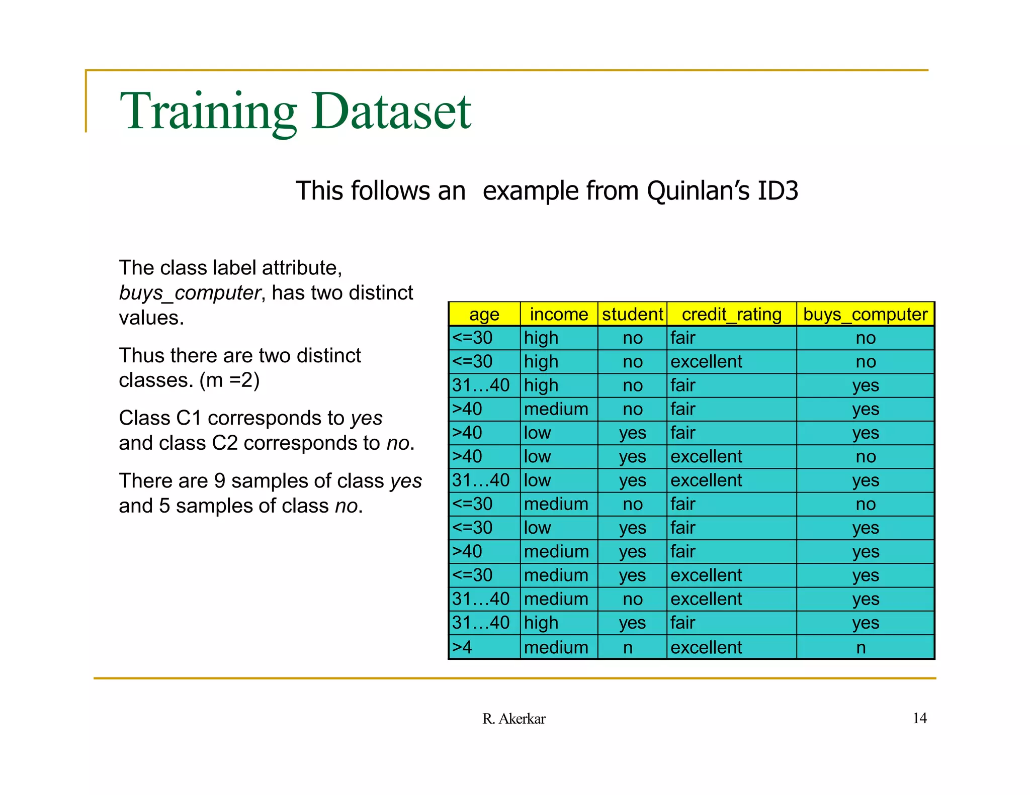
 Example: Let a set of examples consists of 9 instances for class positive,
and 5 instances for class negative.
 Answer: p = 9 and n = 5.
 So Entropy(S) = - (9/14).log2(9/14) - (5/14).log2(5/14)



= -(0.64286)(-0.6375) - (0.35714)(-1.48557)
= (0.40982) + (0.53056)
= 0.940
19
R. Akerkar

20. Entropy
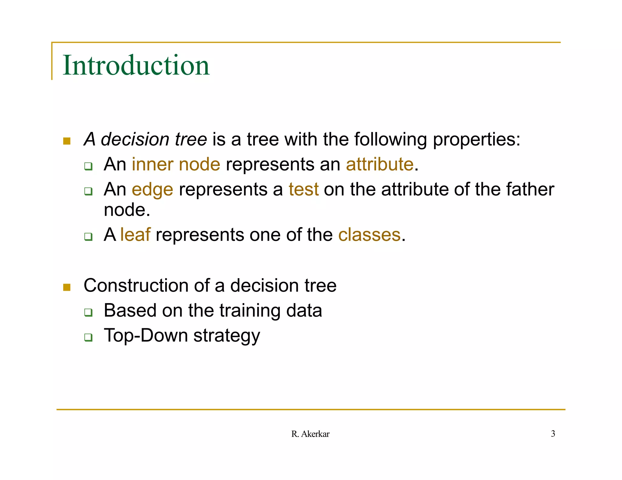
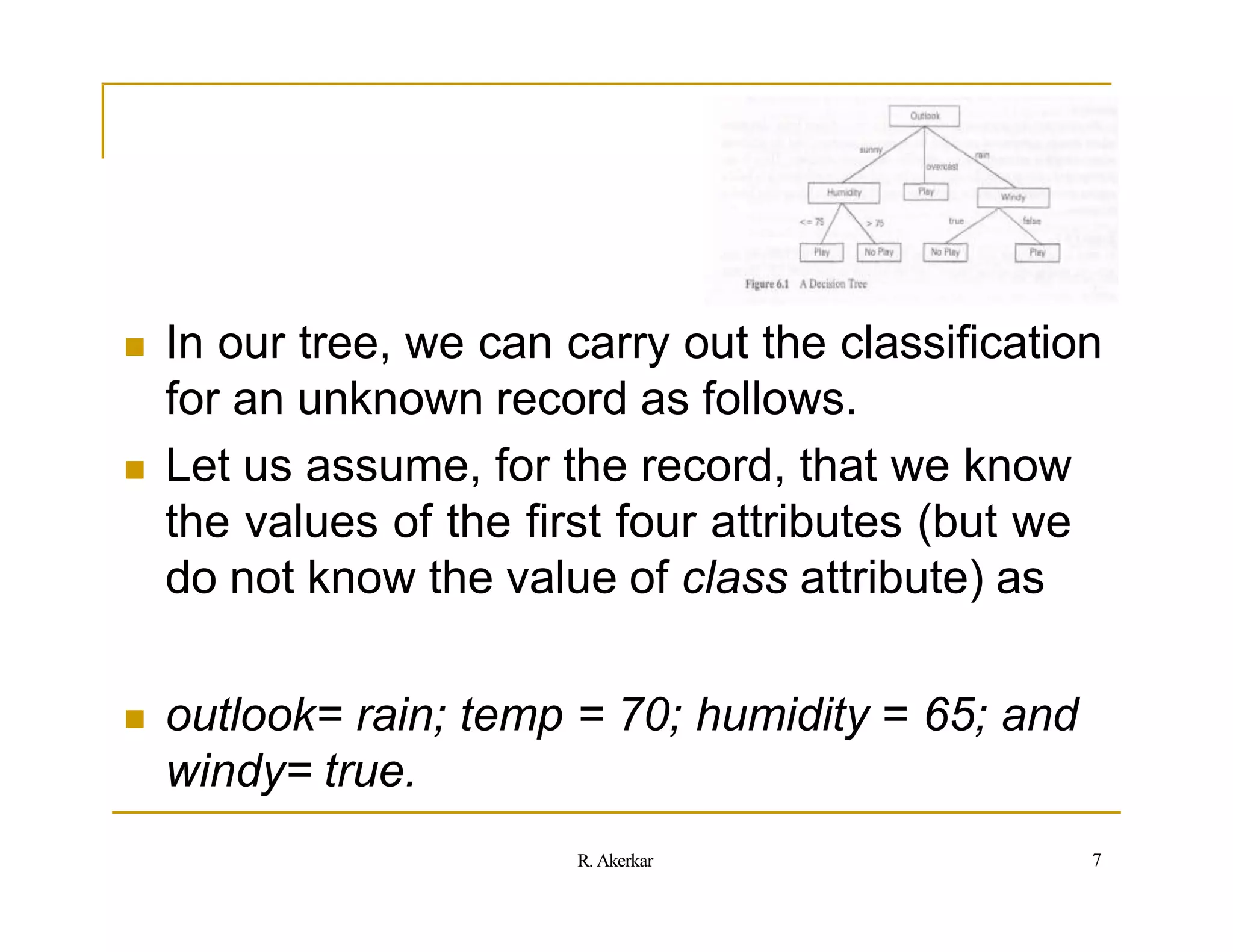
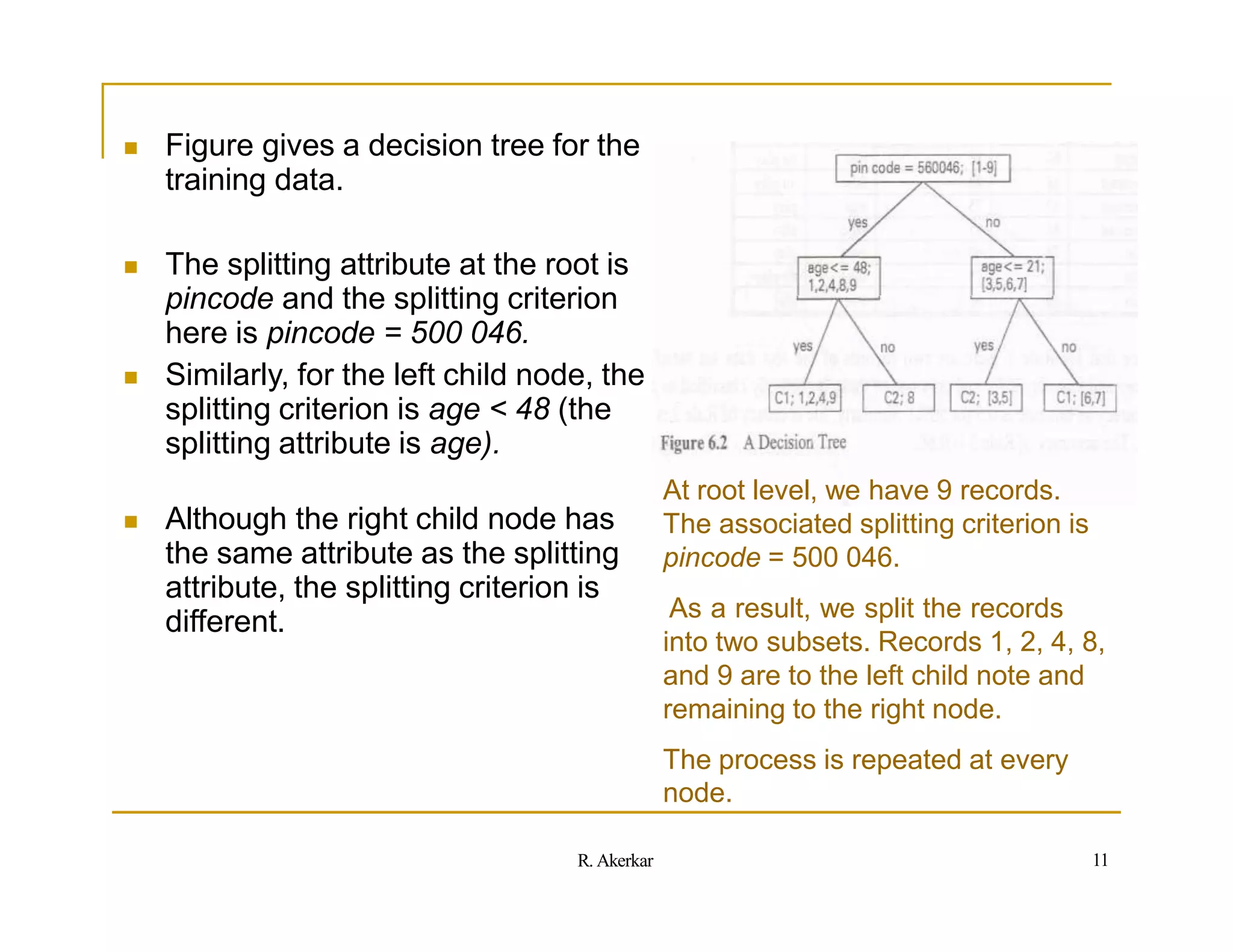
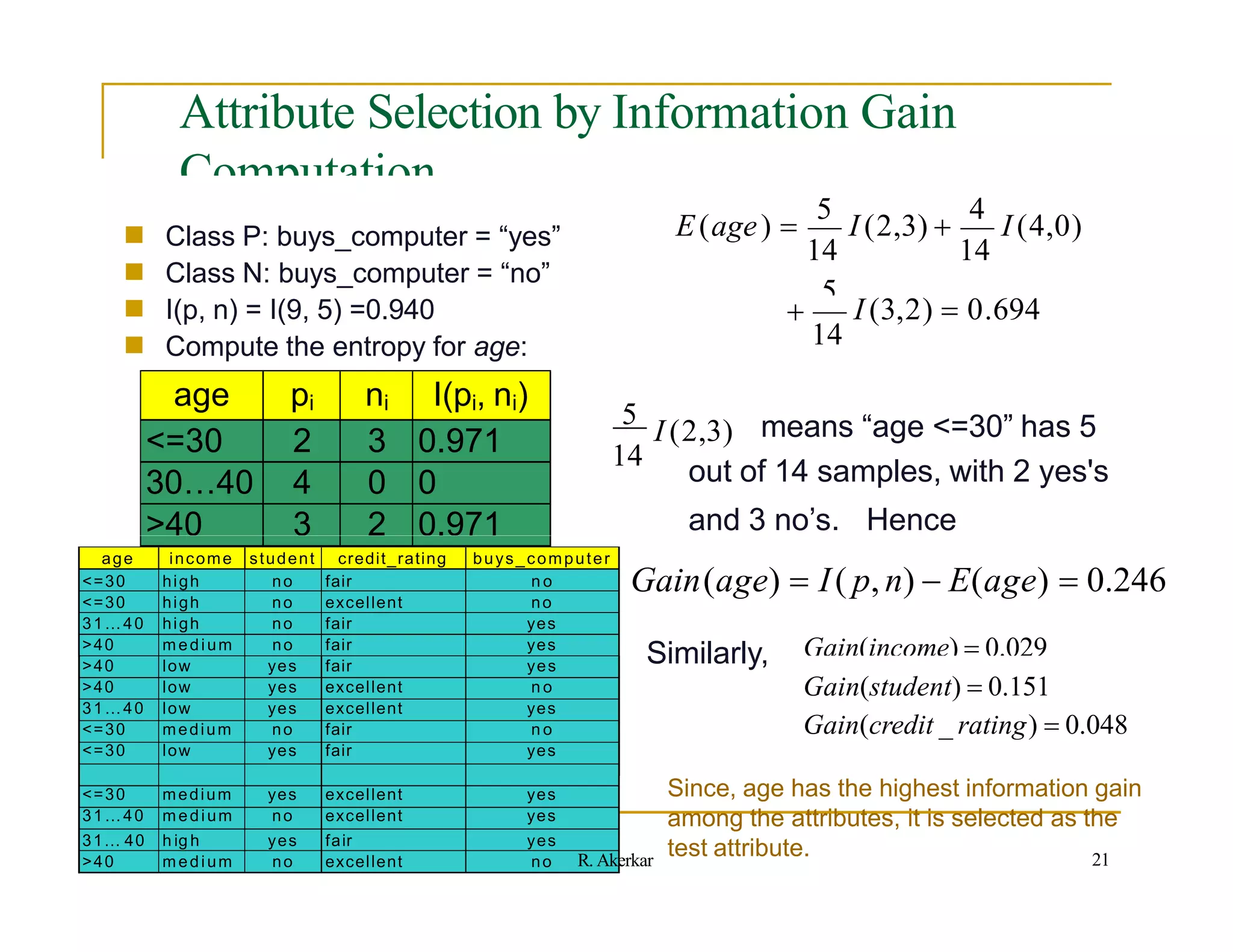
The entropy for a completely pure set is 0 and is 1 for a set with
equal occurrences for both the classes.
i.e. Entropy[14,0] = - (14/14).log2(14/14) - (0/14).log2(0/14)
= -1.log2(1) - 0.log2(0)
= -1.0 - 0
= 0
i.e. Entropy[7,7] = - (7/14).log2(7/14) - (7/14).log2(7/14)
= - (0.5).log2(0.5) - (0.5).log2(0.5)
= - (0.5).(-1) - (0.5).(-1)
= 0.5 + 0.5
= 1
20
R. Akerkar

21. Attribute Selection by Information Gain
Computation
14
5
E(age) 
5
I (2,3) 
4
I (4,0)
14

14
I (3,2)  0.694
means “age <=30” has 5
out of 14 samples, with 2 yes's
and 3 no’s. Hence
 Class P: buys_computer = “yes”
 Class N: buys_computer = “no”
 I(p, n) = I(9, 5) =0.940
 Compute the entropy for age:
age pi ni I(pi, ni)
<=30 2 3 0.971
30…40 4 0 0
>40 3 2 0.971
14
5
I (2,3)
Gain(income)  0.029
Gain(age)  I( p, n)  E(age)  0.246
Similarly,
Gain(student)  0.151
Gain(credit _ rating)  0.048
age income student credit_rating buys_computer
<=30 high no fair n o
<=30 high no excellent no
31…40 high no fair yes
>40 medium no fair yes
>40 low yes fair yes
>40 low yes excellent n o
31…40 low yes excellent yes
<=30 medium no fair n o
<=30 low yes fair yes
<=30 medium yes excellent yes
31…40 medium no excellent yes
31… 40 h ig h yes fair yes
>40 medium no excellent no
Since, age has the highest information gain
among the attributes, it is selected as the
test attribute. 21
R. Akerkar

22. Exercise 1
 The following table consists of training data from an employee
database.
 Let status be the class attribute. Use the ID3 algorithm to construct a
decision tree from the given data.
22
R. Akerkar

23. Solution 1
23
R. Akerkar

24. Other Attribute Selection Measures
 Gini index (CART, IBM IntelligentMiner)
 All attributes are assumed continuous-valued
 Assume there exist several possible split values for each
attribute
 May need other tools, such as clustering, to get the
possible split values
 Can be modified for categorical attributes
24
R. Akerkar

25. Gini Index (IBM IntelligentMiner)
 If a data set T contains examples from n classes, gini index, gini(T) is
defined as
n
 p 2
j
gini (T )  1 
j 1
where pj is the relative frequency of class j in T.
 If a data set T is split into two subsets T1 and T2 with sizes N1 and N2
respectively, the gini index of the split data contains examples from n
classes, the gini index gini(T) is defined as
gini split (T )  N 1 gini (T1) N 2 gini (T 2)
N N
 The attribute provides the smallest ginisplit(T) is chosen to split the node
(need to enumerate all possible splitting points for each attribute).
25
R. Akerkar

26. Exercise 2
26
R. Akerkar

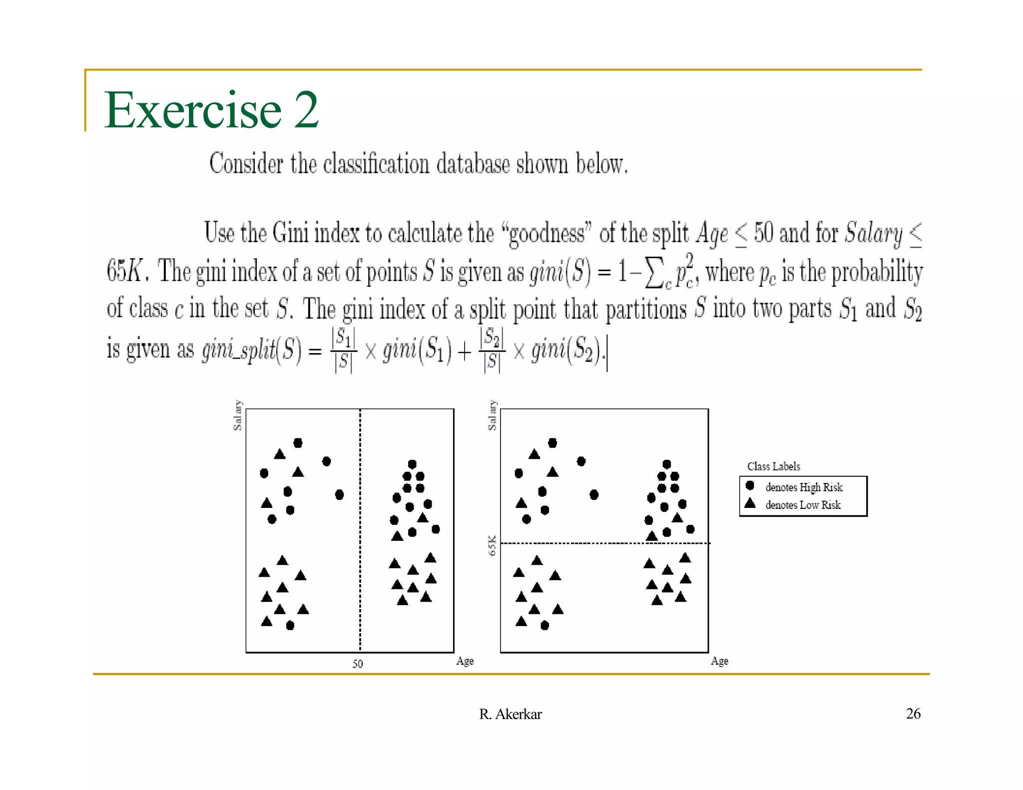
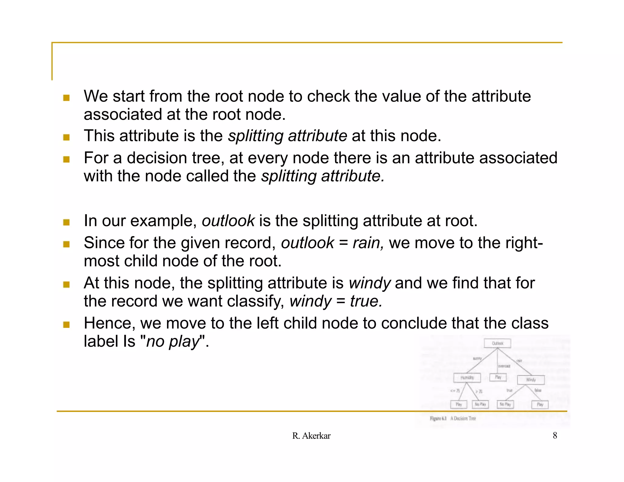
27. Solution 2
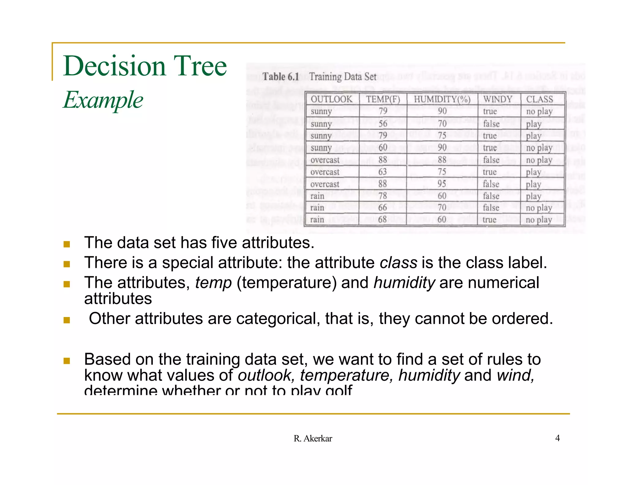
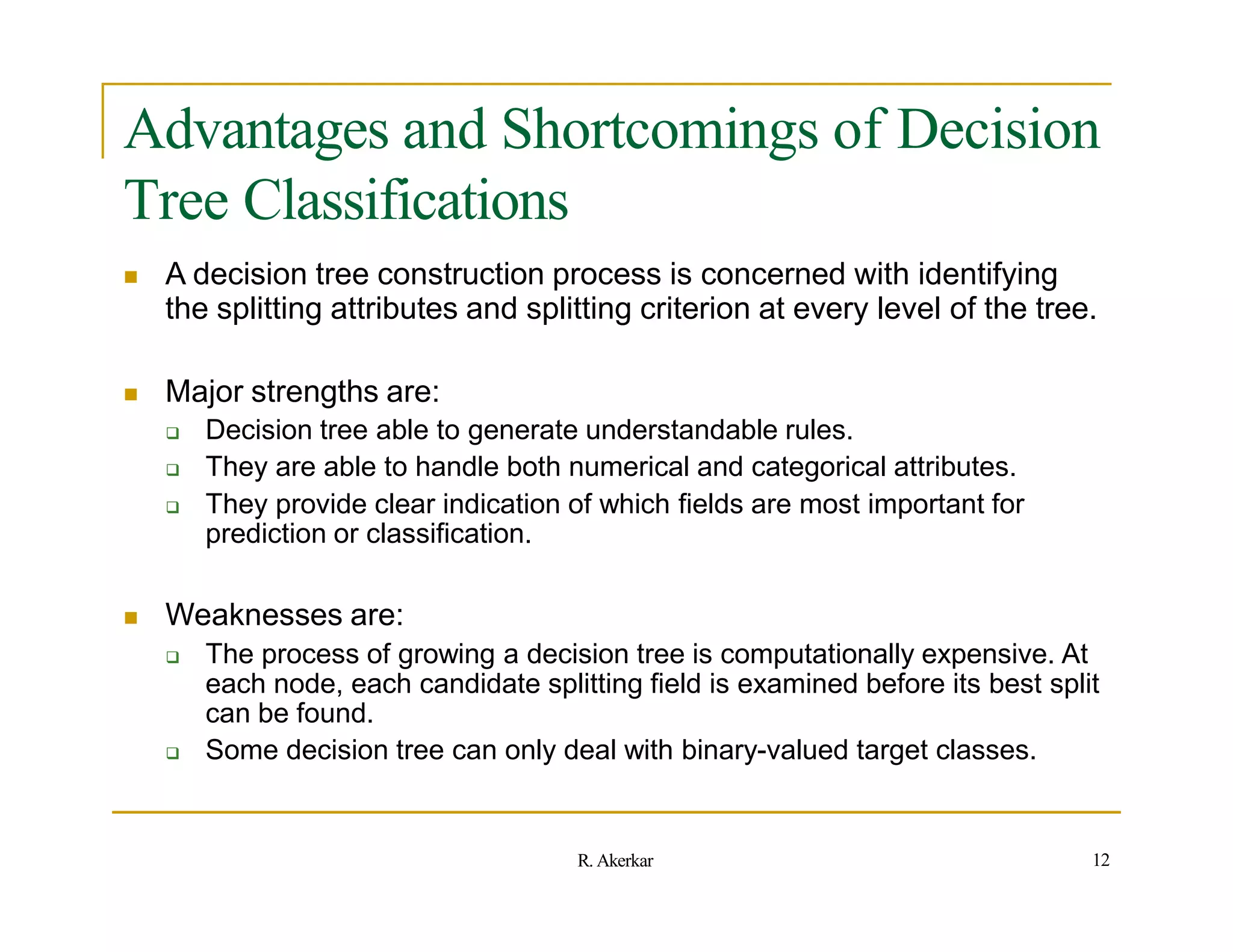
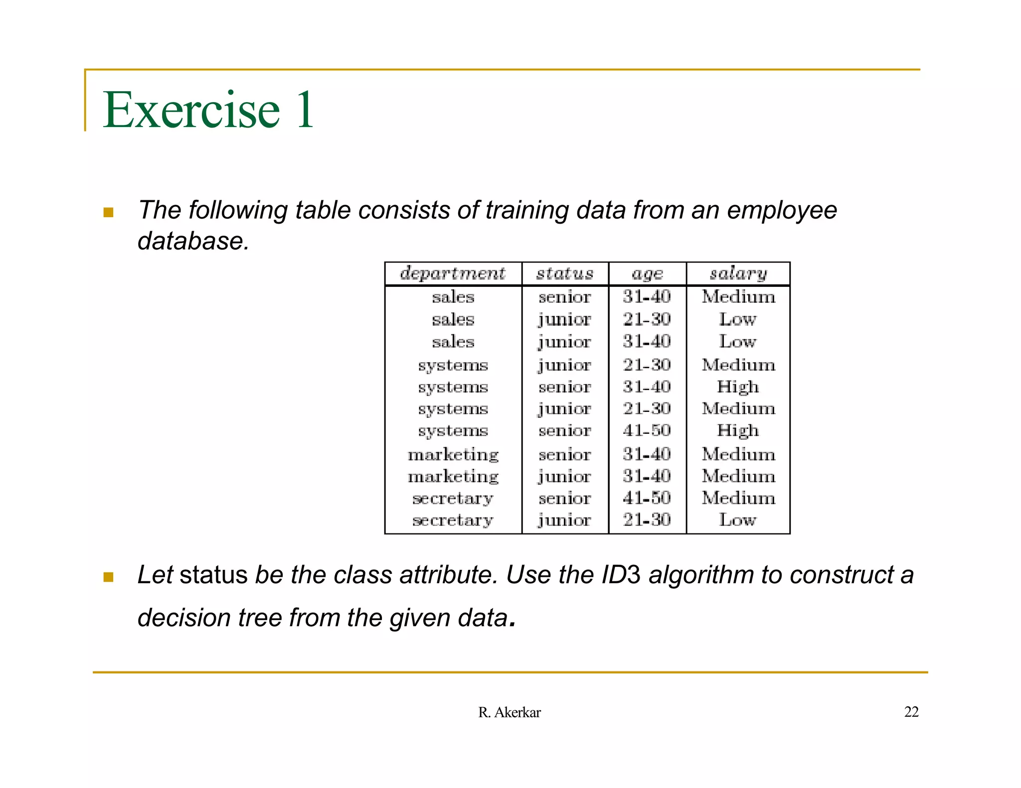
 SPLIT: Age <= 50
 ----------------------
 | High | Low | Total
 --------------------
 S1 (left) | 8 | 11 | 19
 S2 (right) | 11 | 10 | 21

 For S1: P(high) = 8/19 = 0.42 and P(low) = 11/19 = 0.58
 For S2: P(high) = 11/21 = 0.52 and P(low) = 10/21 = 0.48
 Gini(S1) = 1-[0.42x0.42 + 0.58x0.58] = 1-[0.18+0.34] = 1-0.52 = 0.48
 Gini(S2) = 1-[0.52x0.52 + 0.48x0.48] = 1-[0.27+0.23] = 1-0.5 = 0.5
 Gini-Split(Age<=50) = 19/40 x 0.48 + 21/40 x 0.5 = 0.23 + 0.26 = 0.49
 SPLIT: Salary <= 65K
 ----------------------
 | High | Low | Total
 --------------------
 S1 (top) | 18 | 5 | 23
 S2 (bottom) | 1 | 16 | 17
 --------------------
 For S1: P(high) = 18/23 = 0.78 and P(low) = 5/23 = 0.22
 For S2: P(high) = 1/17 = 0.06 and P(low) = 16/17 = 0.94
 Gini(S1) = 1-[0.78x0.78 + 0.22x0.22] = 1-[0.61+0.05] = 1-0.66 = 0.34
 Gini(S2) = 1-[0.06x0.06 + 0.94x0.94] = 1-[0.004+0.884] = 1-0.89 = 0.11
 Gini-Split(Age<=50) = 23/40 x 0.34 + 17/40 x 0.11 = 0.20 + 0.05 = 0.25
27
R. Akerkar

28. Exercise 3
 In previous exercise, which is a better split of
the data among the two split points? Why?
28
R. Akerkar

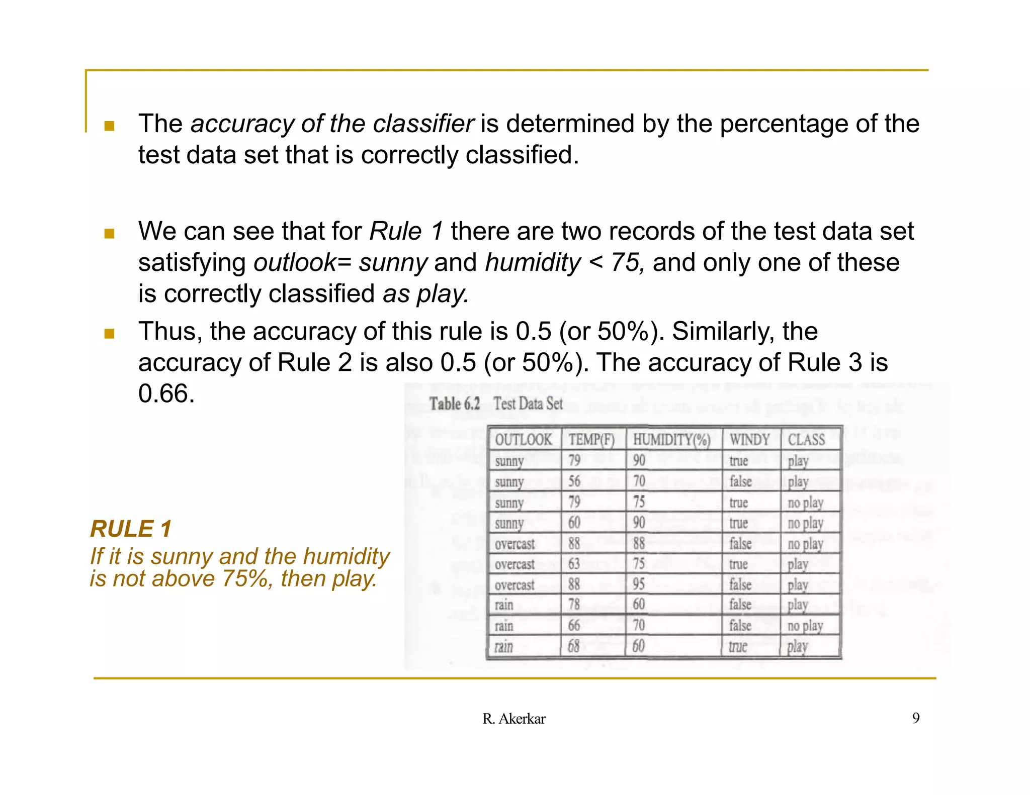
29. Solution 3
``
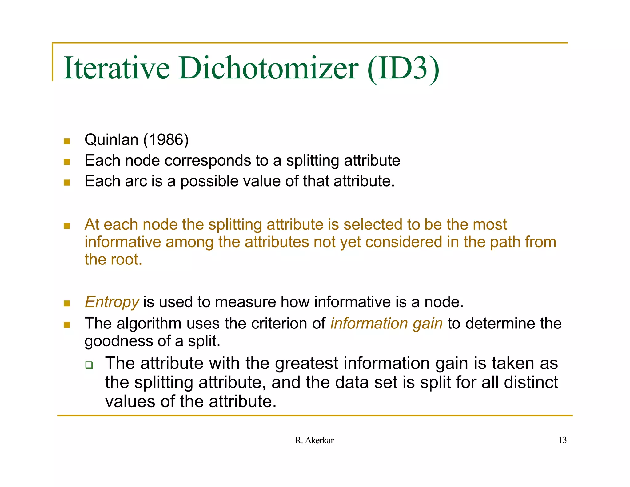
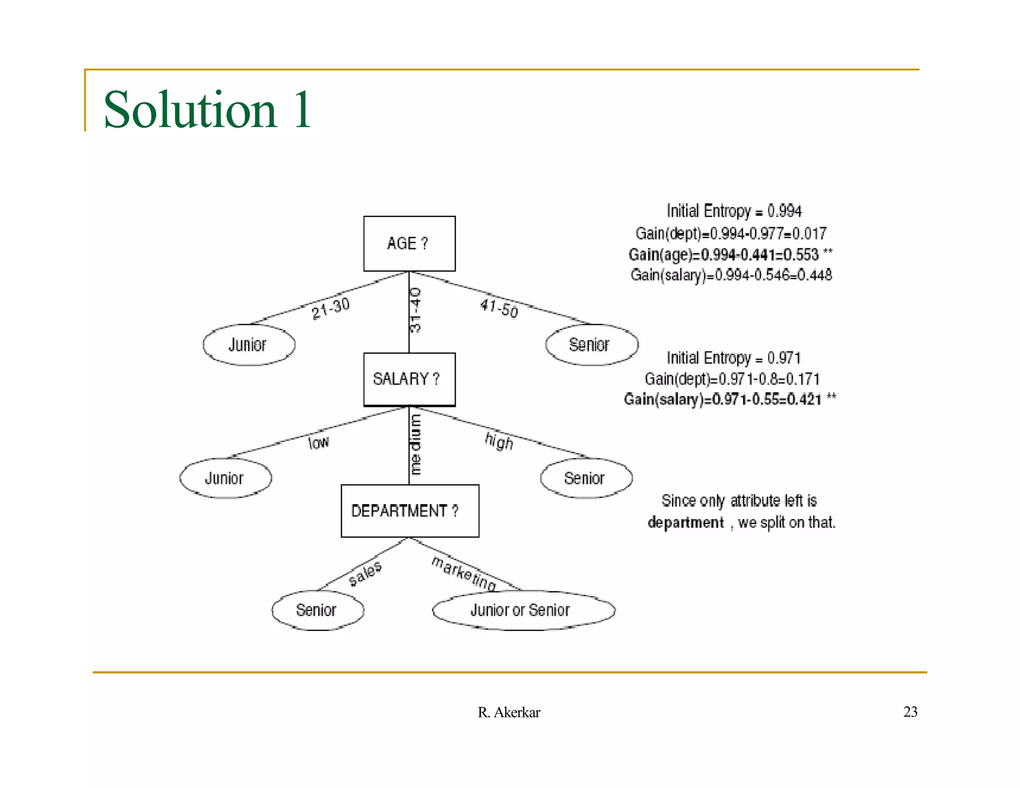
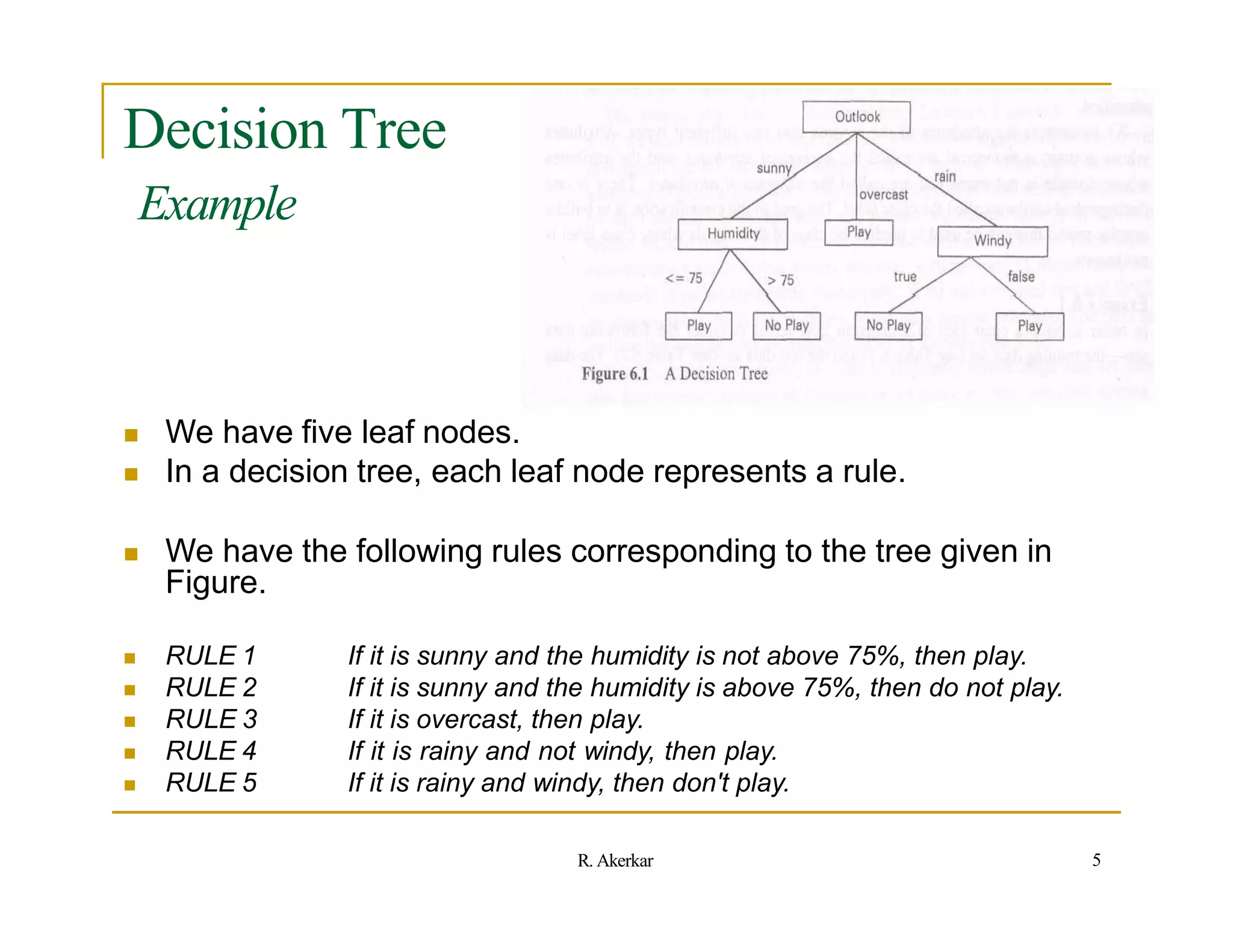
 Intuitively Salary <= 65K is a better split point since it produces
relatively pure'' partitions as opposed to Age <= 50, which
results in more mixed partitions (i.e., just look at the distribution
of Highs and Lows in S1 and S2).
 More formally, let us consider the properties of the Gini index.
If a partition is totally pure, i.e., has all elements from the same
class, then gini(S) = 1-[1x1+0x0] = 1-1 = 0 (for two classes).
On the other hand if the classes are totally mixed, i.e., both
classes have equal probability then
gini(S) = 1 - [0.5x0.5 + 0.5x0.5] = 1-[0.25+0.25] = 0.5.
In other words the closer the gini value is to 0, the better the
partition is. Since Salary has lower gini it is a better split.
29
R. Akerkar

30. Avoid Overfitting in Classification
 Overfitting: An induced tree may overfit the training data
 Too many branches, some may reflect anomalies due to noise
or outliers
 Poor accuracy for unseen samples
 Two approaches to avoid overfitting
 Prepruning: Halt tree construction early—do not split a node if
this would result in the goodness measure falling below a
threshold
 Difficult to choose an appropriate threshold
 Postpruning: Remove branches from a “fully grown” tree—get a
sequence of progressively pruned trees
 Use a set of data different from the training data to decide
which is the “best pruned tree”
30
R. Akerkar