CPM and PERT are project management techniques that use network diagrams to analyze the tasks, schedule, and dependencies of a project. They determine the critical path, which is the longest sequence of tasks that determines the minimum time to complete the project. PERT further accounts for uncertainty in task durations by using three time estimates to calculate the expected duration and variance for each task. This allows calculating the probability of completing the project by a given date.
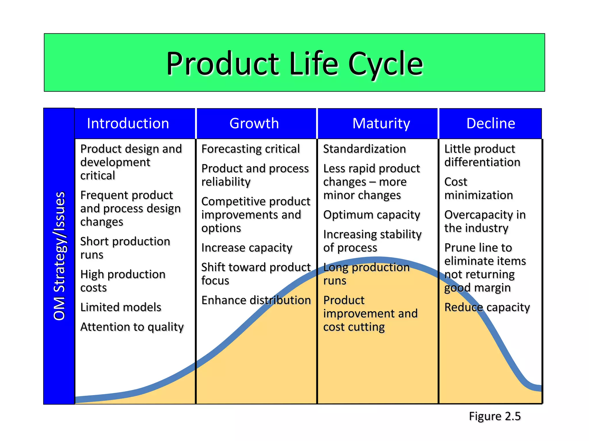
Discusses the stages of Product Life Cycle: Introduction, Growth, Maturity, Decline; strategies for market share, cost control, and design changes.
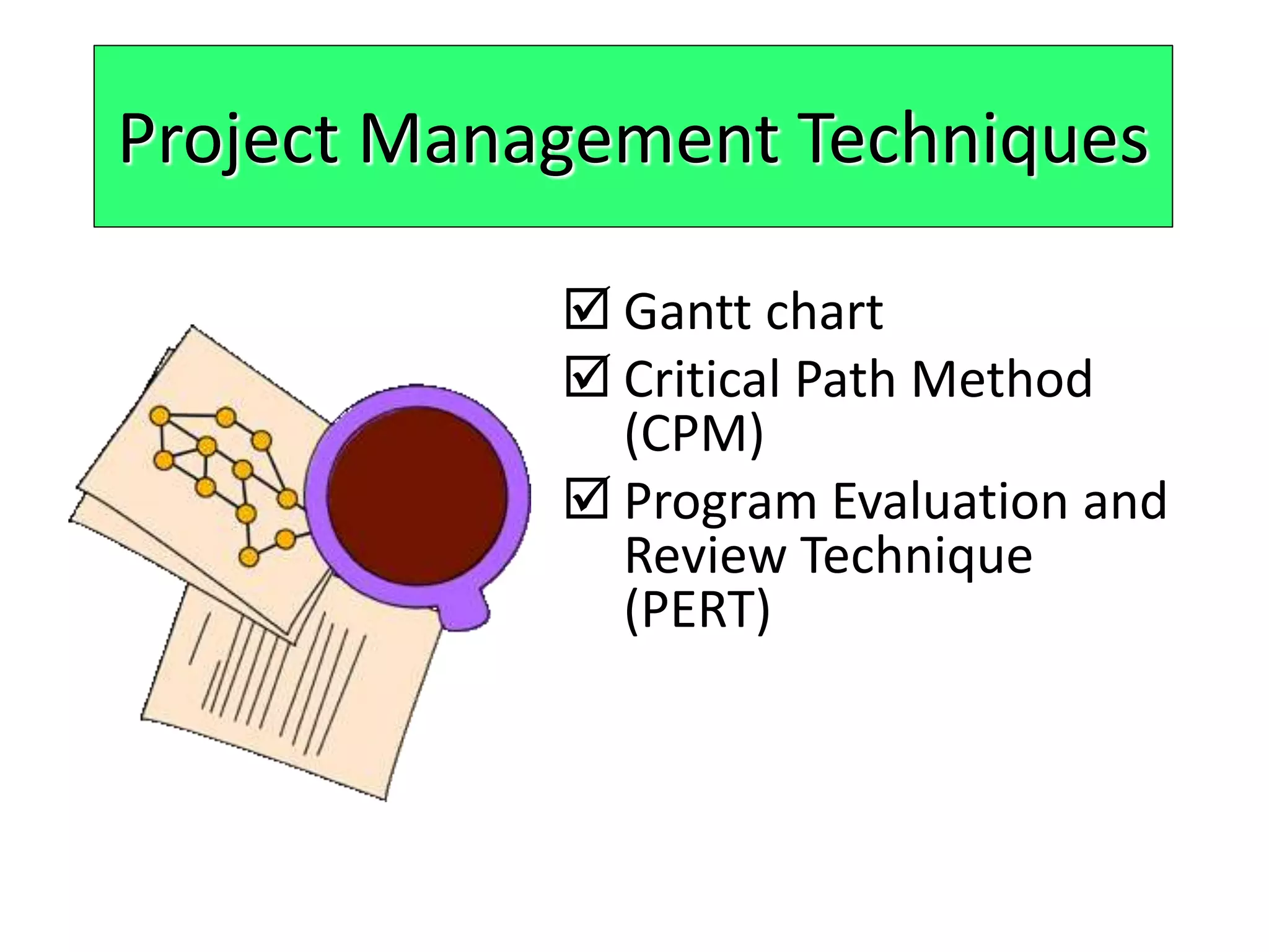
Introduces Gantt charts, CPM and PERT; discusses their development history and use in project management.
Details six steps to implement PERT and CPM for project management including defining the project, estimating time/cost, and critical path analysis.
Identifies important questions that CPM and PERT can answer regarding project timing, resource allocation, and budget management.
Focuses on critical path analysis, defines terms like earliest start/finish and latest start/finish, and provides an example of project activity timeline.
Explains forward pass method; calculating earliest start and finish times for project activities.
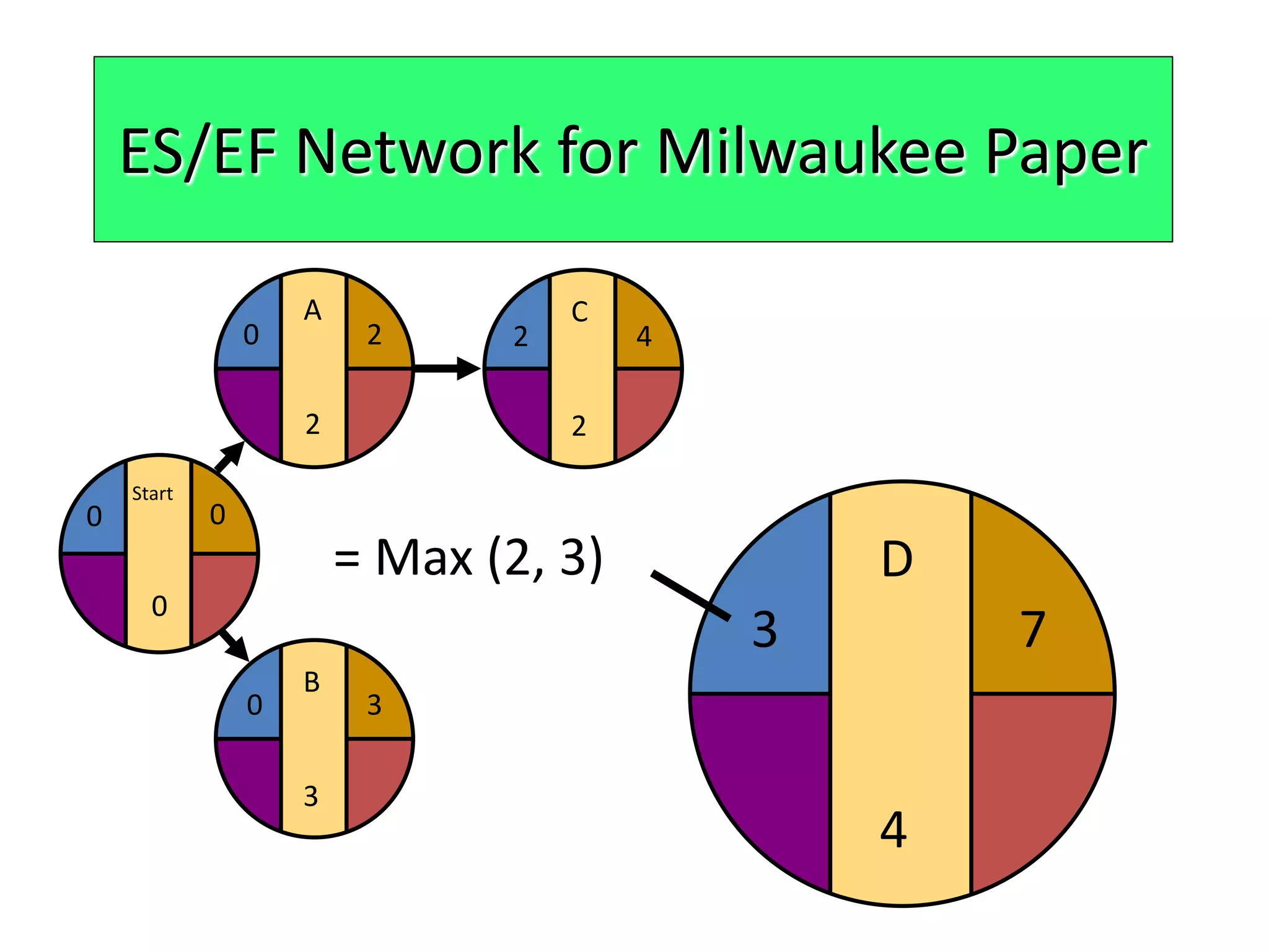
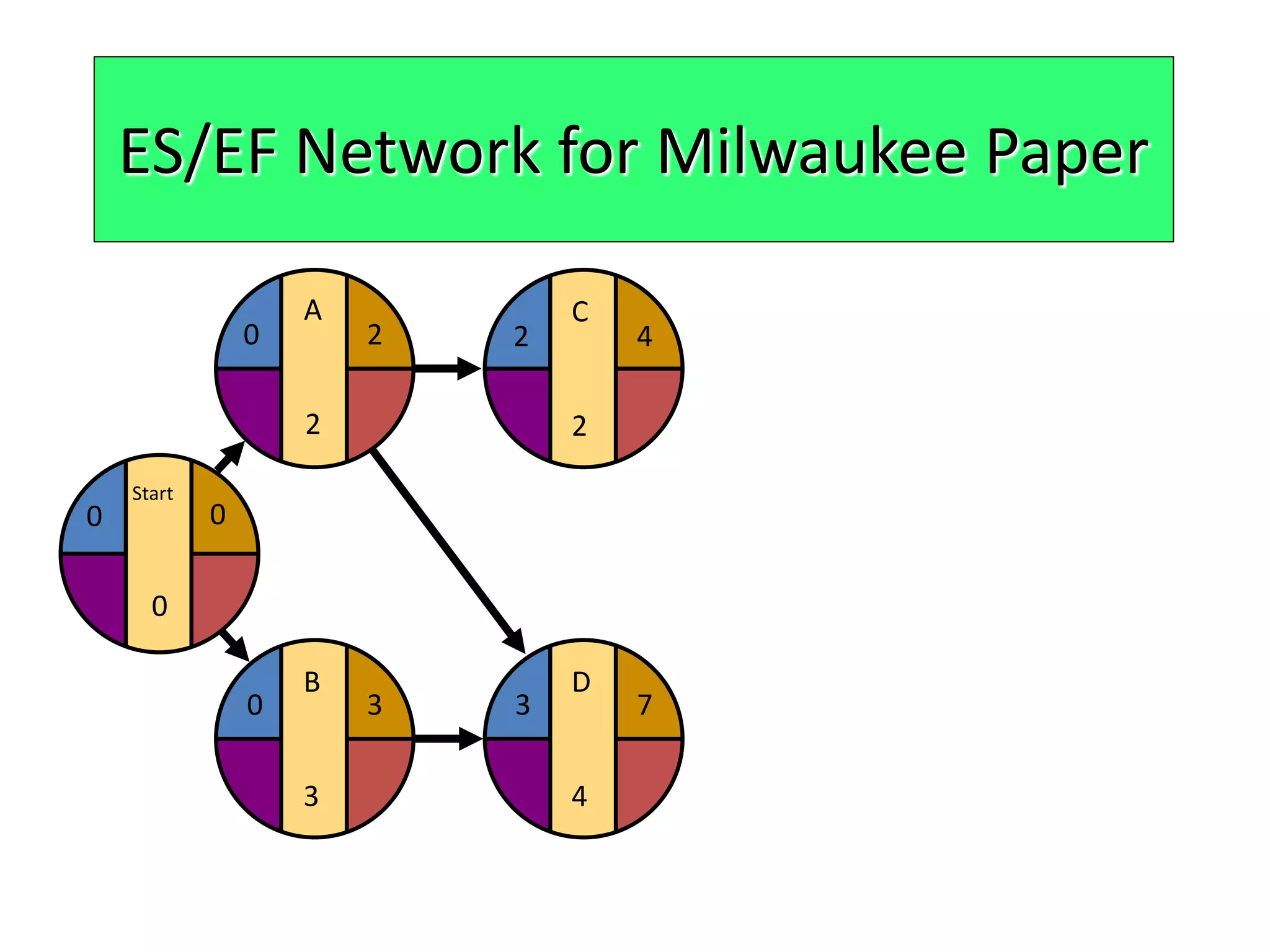
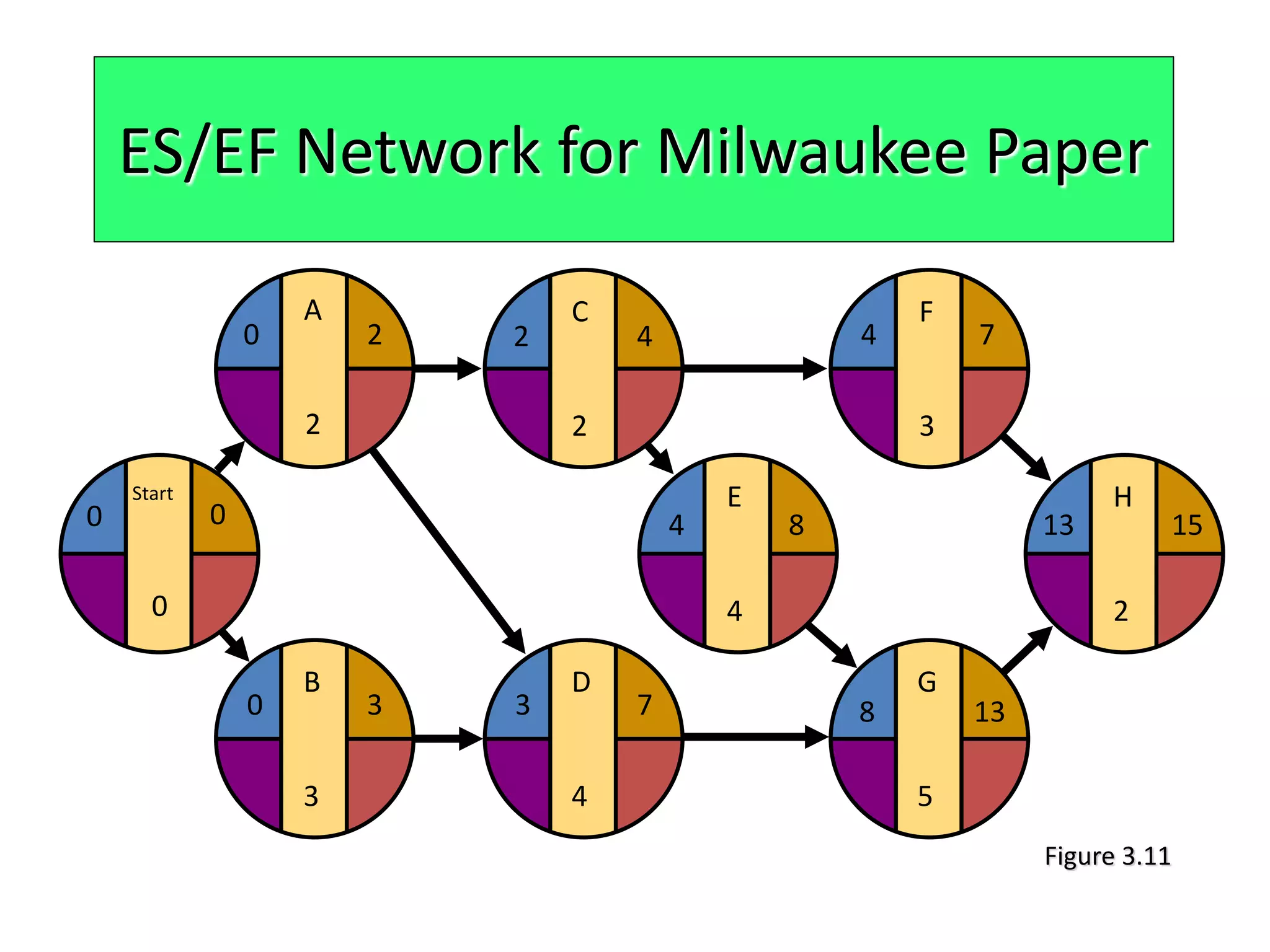
Illustrates ES/EF calculations for activities in a project network diagram related to a Milwaukee Paper project.
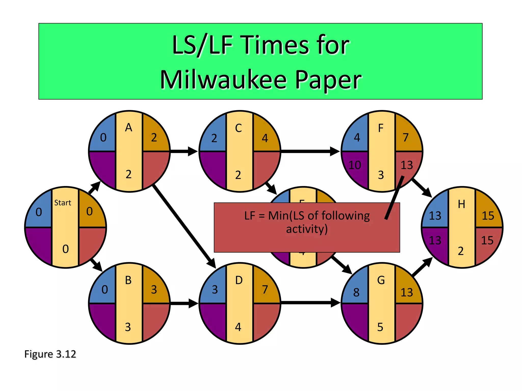
Details backward pass method; calculations for latest finish and start times, as well as their implications for project scheduling.
Presents LS and LF calculations for project activities; analyzes the relationships between these calculations and project duration.
Defines slack time and provides a table for calculating slack, showcasing critical and non-critical paths.
Illustrates the critical path for Milwaukee Paper project; summarizes dependencies and scheduling for activities.
Contrasts CPM and PERT; describes how variability affects project timelines and the need for multiple time estimates.
Explains the statistical approach to estimating project durations using a beta distribution and evaluates project probabilities.
Calculates project variance and standard deviation using critical path activities to assess project completion probability.
Discusses the benefits of PERT/CPM for project management, while acknowledging limitations that may affect accuracy.
Product Life Cycle
Bestperiod to
increase market share
R&D engineering is
critical
Practical to change
price or quality image
Strengthen niche
Poor time to change
image, price, or quality
Competitive costs
become critical
Defend market
position
Cost control critical
Introduction Growth Maturity Decline
CompanyStrategy/Issues
Internet
Flat-screen
monitors
Sales
DVD
CD-ROM
Drive-through
restaurants
Fax machines
3 1/2”
Floppy
disks
Color printers
Figure 2.5
3.
Product Life Cycle
Productdesign and
development
critical
Frequent product
and process design
changes
Short production
runs
High production
costs
Limited models
Attention to quality
Introduction Growth Maturity Decline
OMStrategy/Issues
Forecasting critical
Product and process
reliability
Competitive product
improvements and
options
Increase capacity
Shift toward product
focus
Enhance distribution
Standardization
Less rapid product
changes – more
minor changes
Optimum capacity
Increasing stability
of process
Long production
runs
Product
improvement and
cost cutting
Little product
differentiation
Cost
minimization
Overcapacity in
the industry
Prune line to
eliminate items
not returning
good margin
Reduce capacity
Figure 2.5
4.
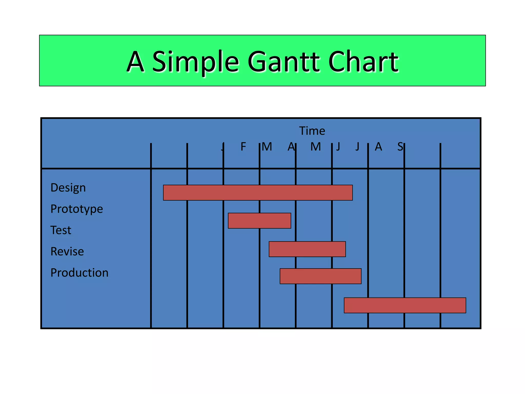
Gantt chart
Critical Path Method
(CPM)
Program Evaluation and
Review Technique
(PERT)
Project Management Techniques
5.
A Simple GanttChart
Time
J F M A M J J A S
Design
Prototype
Test
Revise
Production
6.
Network techniques
Developed in 1950’s
CPM by DuPont for chemical plants (1957)
PERT by Booz, Allen & Hamilton with the U.S.
Navy, for Polaris missile (1958)
Consider precedence relationships and
interdependencies
Each uses a different estimate of activity times
PERT and CPM
7.
Six Steps PERT& CPM
1. Define the project and prepare the work
breakdown structure
2. Develop relationships among the activities
- decide which activities must precede and
which must follow others
3. Draw the network connecting all of the
activities
8.
Six Steps PERT& CPM
4. Assign time and/or cost estimates to each
activity
5. Compute the longest time path through
the network – this is called the critical
path
6. Use the network to help plan, schedule,
monitor, and control the project
9.
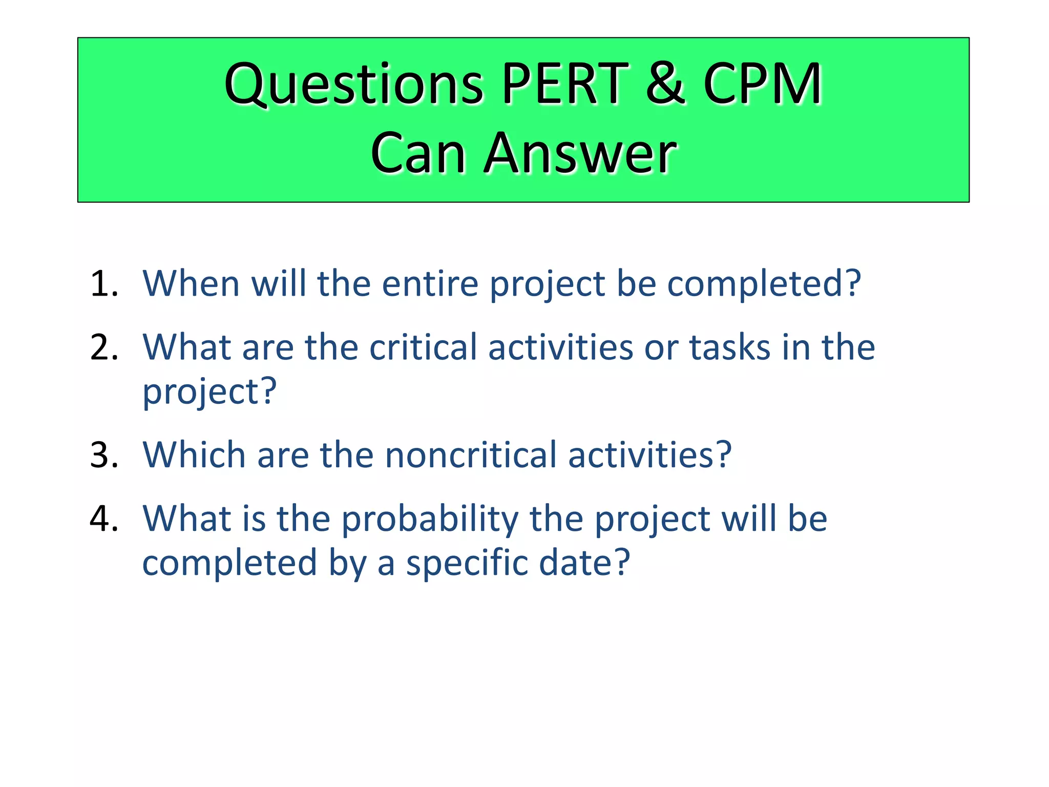
1. When willthe entire project be completed?
2. What are the critical activities or tasks in the
project?
3. Which are the noncritical activities?
4. What is the probability the project will be
completed by a specific date?
Questions PERT & CPM
Can Answer
10.
5. Is theproject on schedule, behind schedule, or
ahead of schedule?
6. Is the money spent equal to, less than, or greater
than the budget?
7. Are there enough resources available to finish
the project on time?
8. If the project must be finished in a shorter time,
what is the way to accomplish this at least cost?
Questions PERT & CPM
Can Answer
11.
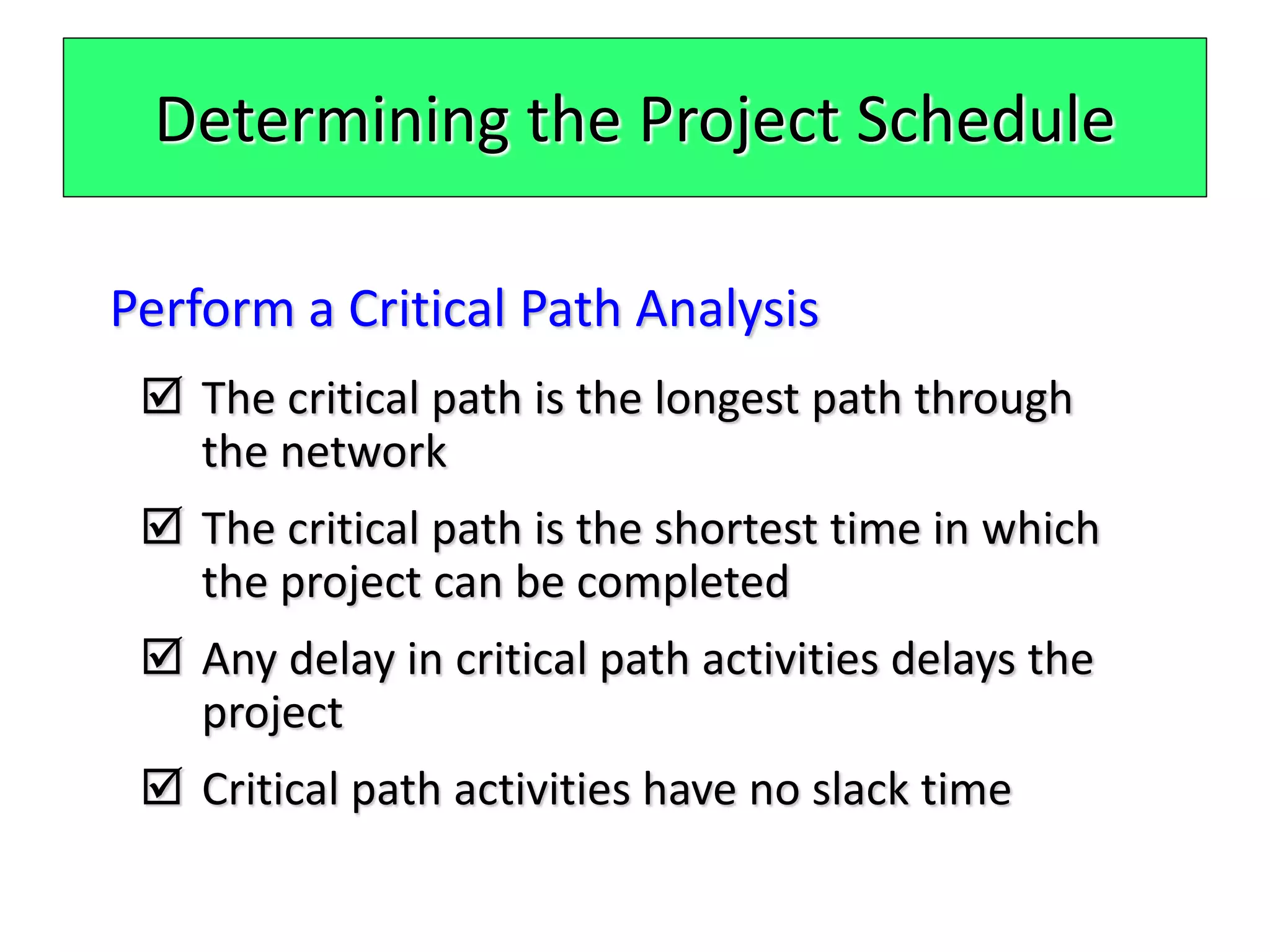
Determining the ProjectSchedule
Perform a Critical Path Analysis
The critical path is the longest path through
the network
The critical path is the shortest time in which
the project can be completed
Any delay in critical path activities delays the
project
Critical path activities have no slack time
12.
Determining the ProjectSchedule
Perform a Critical Path Analysis
Activity Description Time (weeks)
A Build internal components 2
B Modify roof and floor 3
C Construct collection stack 2
D Pour concrete and install frame 4
E Build high-temperature burner 4
F Install pollution control system 3
G Install air pollution device 5
H Inspect and test 2
Total Time (weeks) 25
Table 3.2
13.
Determining the ProjectSchedule
Perform a Critical Path Analysis
Table 3.2
Activity Description Time (weeks)
A Build internal components 2
B Modify roof and floor 3
C Construct collection stack 2
D Pour concrete and install frame 4
E Build high-temperature burner 4
F Install pollution control system 3
G Install air pollution device 5
H Inspect and test 2
Total Time (weeks) 25
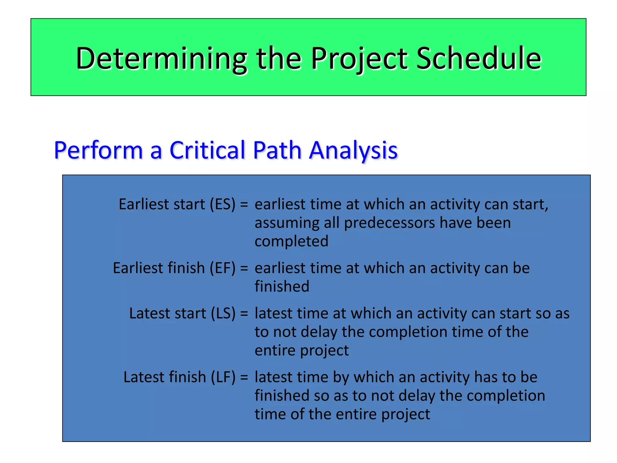
Earliest start (ES) = earliest time at which an activity can start,
assuming all predecessors have been
completed
Earliest finish (EF) = earliest time at which an activity can be
finished
Latest start (LS) = latest time at which an activity can start so as
to not delay the completion time of the
entire project
Latest finish (LF) = latest time by which an activity has to be
finished so as to not delay the completion
time of the entire project
14.
Determining the ProjectSchedule
Perform a Critical Path Analysis
Figure 3.10
A
Activity Name or
Symbol
Earliest Start
ES
Earliest Finish
EF
Latest Start LS Latest FinishLF
Activity Duration
2
15.
Forward Pass
Begin atstarting event and work forward
Earliest Start Time Rule:
If an activity has only one immediate predecessor, its ES equals
the EF of the predecessor
If an activity has multiple immediate predecessors, its ES is the
maximum of all the EF values of its predecessors
ES = Max (EF of all immediate predecessors)
16.
Forward Pass
Begin atstarting event and work forward
Earliest Finish Time Rule:
The earliest finish time (EF) of an activity is the sum of its
earliest start time (ES) and its activity time
EF = ES + Activity time
17.
ES/EF Network forMilwaukee Paper
Start
0
0
ES
0
EF = ES + Activity time
18.
ES/EF Network forMilwaukee Paper
Start
0
0
0
A
2
2
EF of A =
ES of A + 2
0
ES
of A
19.
B
3
ES/EF Network forMilwaukee Paper
Start
0
0
0
A
2
20
3
EF of B =
ES of B + 3
0
ES
of B
E
4
F
3
G
5
H
2
4 8 1315
4
8 13
7
D
4
3 7
C
2
2 4
ES/EF Network for Milwaukee Paper
B
3
0 3
Start
0
0
0
A
2
20
Figure 3.11
24.
Backward Pass
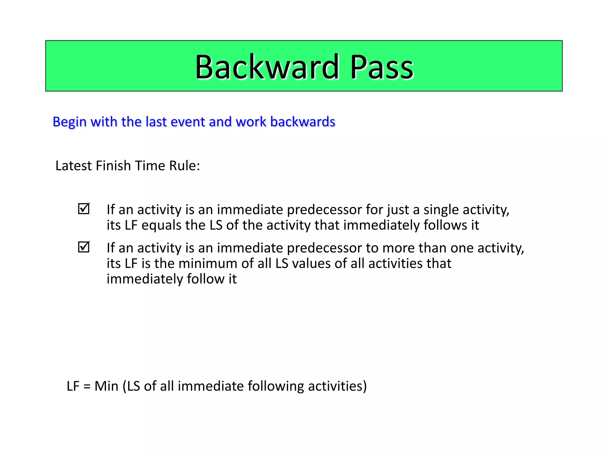
Begin withthe last event and work backwards
Latest Finish Time Rule:
If an activity is an immediate predecessor for just a single activity,
its LF equals the LS of the activity that immediately follows it
If an activity is an immediate predecessor to more than one activity,
its LF is the minimum of all LS values of all activities that
immediately follow it
LF = Min (LS of all immediate following activities)
25.
Backward Pass
Begin withthe last event and work backwards
Latest Start Time Rule:
The latest start time (LS) of an activity is the difference of its latest
finish time (LF) and its activity time
LS = LF – Activity time
26.
LS/LF Times for
MilwaukeePaper
E
4
F
3
G
5
H
2
4 8 13 15
4
8 13
7
D
4
3 7
C
2
2 4
B
3
0 3
Start
0
0
0
A
2
20
Figure 3.12
LF = EF
of Project
1513
LS = LF – Activity time
27.
LS/LF Times for
MilwaukeePaper
E
4
F
3
G
5
H
2
4 8 13 15
4
8 13
7
13 15
D
4
3 7
C
2
2 4
B
3
0 3
Start
0
0
0
A
2
20
LF = Min(LS of following
activity)
10 13
Figure 3.12
28.
LS/LF Times for
MilwaukeePaper
E
4
F
3
G
5
H
2
4 8 13 15
4
8 13
7
13 15
10 13
8 13
4 8
D
4
3 7
C
2
2 4
B
3
0 3
Start
0
0
0
A
2
20
LF = Min(4, 10)
42
Figure 3.12
29.
LS/LF Times for
MilwaukeePaper
E
4
F
3
G
5
H
2
4 8 13 15
4
8 13
7
13 15
10 13
8 13
4 8
D
4
3 7
C
2
2 4
B
3
0 3
Start
0
0
0
A
2
20
42
84
20
41
00
Figure 3.12
30.
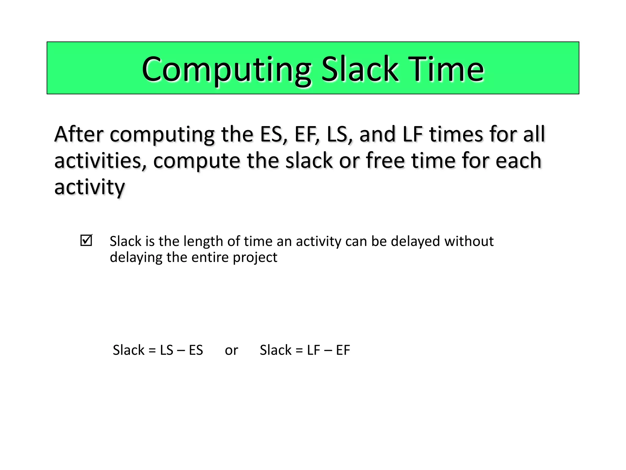
Computing Slack Time
Aftercomputing the ES, EF, LS, and LF times for all
activities, compute the slack or free time for each
activity
Slack is the length of time an activity can be delayed without
delaying the entire project
Slack = LS – ES or Slack = LF – EF
31.
Computing Slack Time
EarliestEarliest Latest Latest On
Start Finish Start Finish Slack Critical
Activity ES EF LS LF LS – ES Path
A 0 2 0 2 0 Yes
B 0 3 1 4 1 No
C 2 4 2 4 0 Yes
D 3 7 4 8 1 No
E 4 8 4 8 0 Yes
F 4 7 10 13 6 No
G 8 13 8 13 0 Yes
H 13 15 13 15 0 Yes
Table 3.3
32.
Critical Path for
MilwaukeePaper
Figure 3.13
E
4
F
3
G
5
H
2
4 8 13 15
4
8 13
7
13 15
10 13
8 13
4 8
D
4
3 7
C
2
2 4
B
3
0 3
Start
0
0
0
A
2
20
42
84
20
41
00
33.
CPM assumeswe know a fixed time
estimate for each activity and there is no
variability in activity times
PERT uses a probability distribution for
activity times to allow for variability
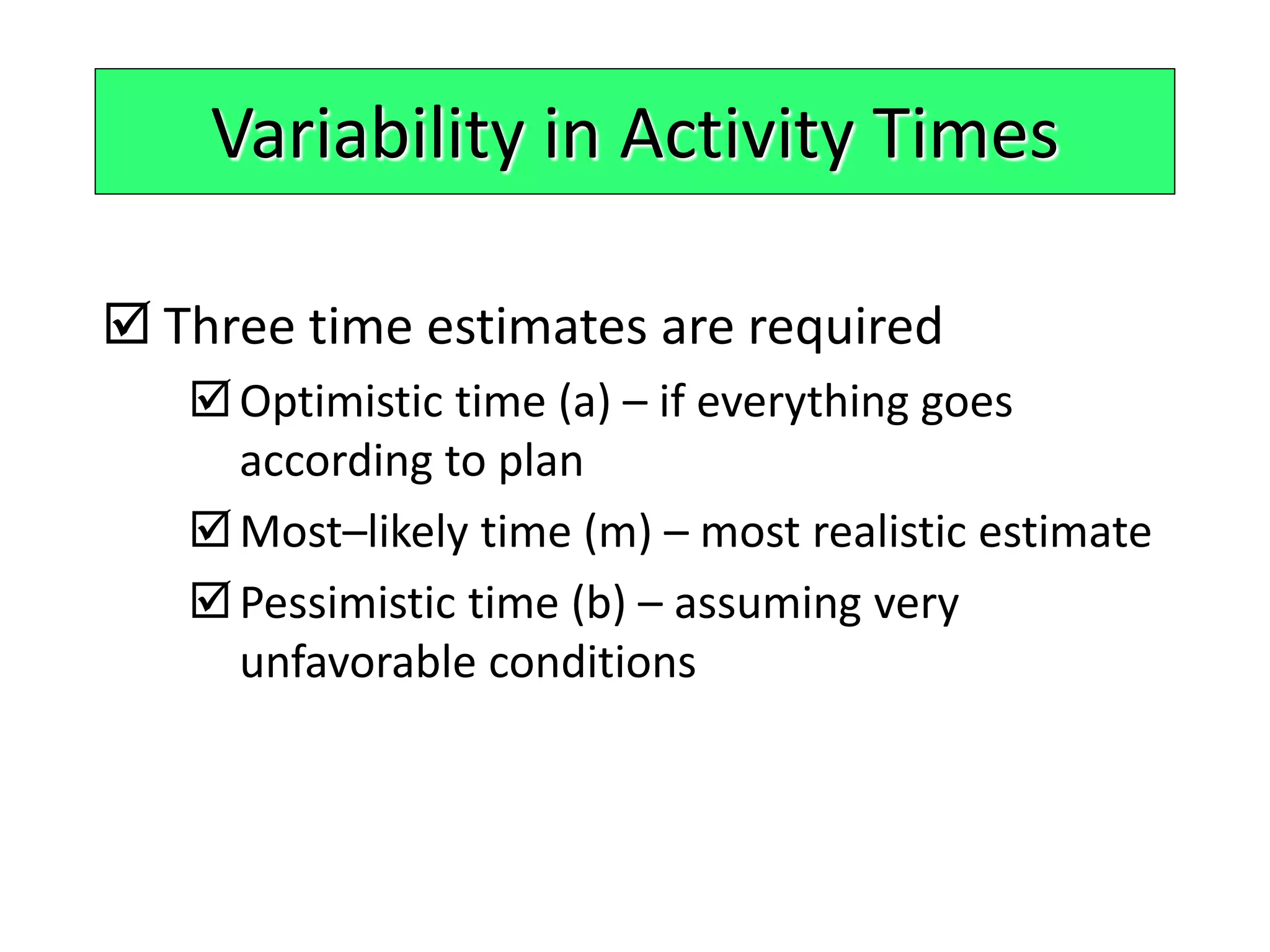
Variability in Activity Times
34.
Three timeestimates are required
Optimistic time (a) – if everything goes
according to plan
Most–likely time (m) – most realistic estimate
Pessimistic time (b) – assuming very
unfavorable conditions
Variability in Activity Times
35.
Estimate follows betadistribution
Variability in Activity Times
Expected time:
Variance of times:
t = (a + 4m + b)/6
v = [(b – a)/6]2
36.
Estimate follows betadistribution
Variability in Activity Times
Expected time:
Variance of times:
t = (a + 4m + b)/6
v = [(b − a)/6]2
Probability of 1
in 100 of > b
occurring
Probability of 1
in 100 of
< a occurring
Probability
Optimistic Time
(a)
Most Likely Time
(m)
Pessimistic Time
(b)
Activity
Time
37.
Computing Variance
Most Expected
OptimisticLikely Pessimistic Time Variance
Activity a m b t = (a + 4m + b)/6 [(b – a)/6]2
A 1 2 3 2 .11
B 2 3 4 3 .11
C 1 2 3 2 .11
D 2 4 6 4 .44
E 1 4 7 4 1.00
F 1 2 9 3 1.78
G 3 4 11 5 1.78
H 1 2 3 2 .11
Table 3.4
38.
Probability of ProjectCompletion
Project variance is computed by
summing the variances of critical
activities
s2 = Project variance
= (variances of activities
on critical path)
p
39.
Probability of ProjectCompletion
Project variance is computed by
summing the variances of critical
activities
Project variance
s2 = .11 + .11 + 1.00 + 1.78 + .11 = 3.11
Project standard deviation
sp = Project variance
= 3.11 = 1.76 weeks
p
40.
Advantages of PERT/CPM
5.Project documentation and graphics point out
who is responsible for various activities
6. Applicable to a wide variety of projects
7. Useful in monitoring not only schedules but
costs as well
41.
1. Project activitieshave to be clearly defined,
independent, and stable in their relationships
2. Precedence relationships must be specified and
networked together
3. Time estimates tend to be subjective and are
subject to fudging by managers
4. There is an inherent danger of too much
emphasis being placed on the longest, or critical,
path
Limitations of PERT/CPM


![Estimate follows beta distribution
Variability in Activity Times
Expected time:
Variance of times:
t = (a + 4m + b)/6
v = [(b – a)/6]2](https://image.slidesharecdn.com/cpmandpert-170521053116/75/Cpm-and-pert-35-2048.jpg)
![Estimate follows beta distribution
Variability in Activity Times
Expected time:
Variance of times:
t = (a + 4m + b)/6
v = [(b − a)/6]2
Probability of 1
in 100 of > b
occurring
Probability of 1
in 100 of
< a occurring
Probability
Optimistic Time
(a)
Most Likely Time
(m)
Pessimistic Time
(b)
Activity
Time](https://image.slidesharecdn.com/cpmandpert-170521053116/75/Cpm-and-pert-36-2048.jpg)
![Computing Variance
Most Expected
Optimistic Likely Pessimistic Time Variance
Activity a m b t = (a + 4m + b)/6 [(b – a)/6]2
A 1 2 3 2 .11
B 2 3 4 3 .11
C 1 2 3 2 .11
D 2 4 6 4 .44
E 1 4 7 4 1.00
F 1 2 9 3 1.78
G 3 4 11 5 1.78
H 1 2 3 2 .11
Table 3.4](https://image.slidesharecdn.com/cpmandpert-170521053116/75/Cpm-and-pert-37-2048.jpg)