The handout of biostatistics

1. Basic Biostatistics
Haramaya University
Collage of Health and Medicine Sciences
School of Public Health
Continuous Data Analysis
By Adisu Birhanu (Assistant prof. of Biostatistics)
Feb 2025

2. Session Objectives
Describe Continuous variable and method of analyses
Describe relationship between continuous variables
Interpret the outputs from linear regression models

3. Analysis of Continuous Data
A continuous variable is one which can take on infinity many,
uncountable possible values in the range of real numbers.
Data analysis methods such as scatter plot, line graphs and
histogram are applicable for describing numerical data.
More advanced methods for inferential analysis of continuous data
include correlation, t-test, ANOVA and linear regression.

4. Comparison of the means
t-test is appropriate to compare two means from two population
There are three different t-tests
One sample t-test
Two independent sample t-test
Paired sample t-test
ANOVA is used for IV with more than two groups
BY ADISU B.

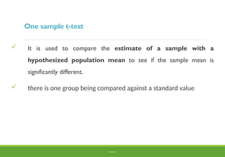
5. One sample t-test
 It is used to compare the estimate of a sample with a
hypothesized population mean to see if the sample mean is
significantly different.
 there is one group being compared against a standard value
BY ADISU B.

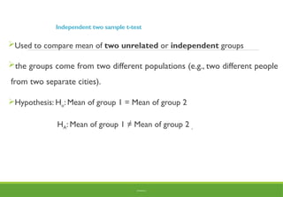
6. Independent two sample t-test
Used to compare mean of two unrelated or independent groups
the groups come from two different populations (e.g., two different people
from two separate cities).
Hypothesis: Ho: Mean of group 1 = Mean of group 2
HA: Mean of group 1 ≠ Mean of group 2 ,
BY ADISU B.

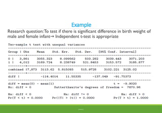
7. Example
Research question:To test if there is significant difference in birth weight of
male and female infant Independent t-test is appropriate
→
BY ADISU B.

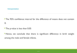
8. Interpretation
The 95% confidence interval for the difference of means does not contain
0.
The p-value is less than 0.05
Hence, we conclude that there is significant difference in birth weight
among the male and female infants.
BY ADISU B.

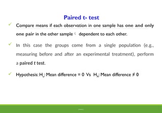
9. Paired t- test
 Compare means if each observation in one sample has one and only
one pair in the other sample dependent to each other.
 In this case the groups come from a single population (e.g.,
measuring before and after an experimental treatment), perform
a paired t test.
 Hypothesis: Ho: Mean difference = 0 Vs HA: Mean difference ≠ 0
BY ADISU B.

10. One wayANOVA (Analysis ofVariance)
For two normal distributions the two sample means are compared by
t-test.
The means of more than two distributions need to be compared.
BY ADISU B.

11. One way ANOVA…
The t-test methodology generalizes to the one-way analysis of variance
(ANOVA) for categorical variables with more than two categories.
ANOVA do not tell you which group is different, but only whether a
difference exists.
To know which group is different, we used post hoc tests (bonferroni,
Tuckey, scheffe).
BY ADISU B.

12. One way ANOVA…
For K means (K> 3).
Ho : µ1 = µ2 = : : : =µ k ,
HA : at least one of the means is different.
There is one factor of grouping (one way ANOVA)
BY ADISU B.

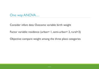
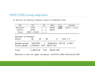
13. One wayANOVA…
Consider infant data: Outcome variable: birth weight
Factor variable: residence (urban= 1, semi-urban= 2, rural=3)
Objective: compare weight among the three place categories
BY ADISU B.

14. STATA CODE:oneway weight place
BY ADISU B.

15. One way ANOVA…
We reject the null hypothesis (p value < 0.05) and
We can conclude that at least one of the groups' means differ on body weight.
Now the question is: which groups are different?
Answering this question requires multiple comparisons (post hoc tests).
Bonferroni,Tukey and scheffe are commonly used methods.
Bonferroni method corrects probability of Type I error for the number of
tests.
BY ADISU B.

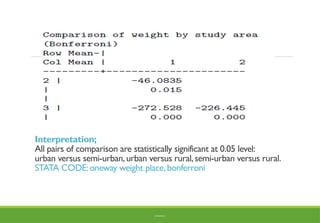
16. Interpretation;
All pairs of comparison are statistically significant at 0.05 level:
urban versus semi-urban,urban versus rural,semi-urban versus rural.
STATA CODE:oneway weight place,bonferroni
BY ADISU B.

17. Correlation
Correlation is used to quantify the degree to which two
continuous random variables are related,
Common correlation measure
Pearson Correlation Coefficient: for linear relationship
between two variables

18. Scatterplot
Helpful tool in exploring relationship between two variables
If No relationship between proposed explanatory and dependent
variables
 Then fitting a linear regression model to data probably will
not provide a useful model
Before attempting to fit a linear model to observed data, a
modeler should first determine whether or not there is a
relationship between the variables of interest
 This does not necessarily imply that one variable causes the
other, but that there is some significant association between the
two variables

19. Scatter plot and correlation of two data

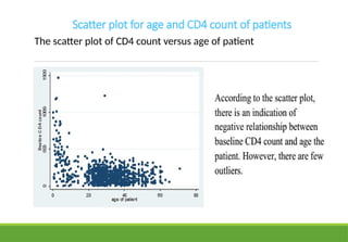
20. Scatter plot for age and CD4 count of patients
The scatter plot of CD4 count versus age of patient

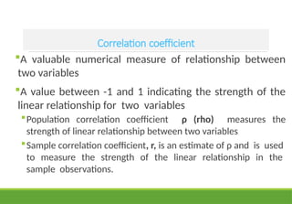
21. Correlation coefficient
A valuable numerical measure of relationship between
two variables
A value between -1 and 1 indicating the strength of the
linear relationship for two variables
Population correlation coefficient ρ (rho) measures the
strength of linear relationship between two variables
Sample correlation coefficient, r, is an estimate of ρ and is used
to measure the strength of the linear relationship in the
sample observations.

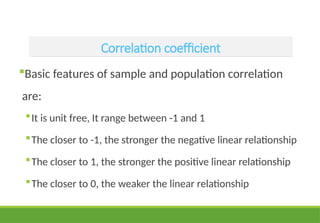
22. Correlation coefficient
Basic features of sample and population correlation
are:
It is unit free, It range between -1 and 1
The closer to -1, the stronger the negative linear relationship
The closer to 1, the stronger the positive linear relationship
The closer to 0, the weaker the linear relationship

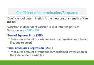
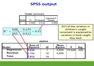
23. Coefficient of determination/R squared
Coefficient of determination is the measure of strength of the
model
Variation in dependent variable is split into two parts as
Variation in y = SSE + SSR
Sum of Squares Error (SSE):
 Measures amount of variation in y that remains unexplained
(i.e. due to error)
Sum of Squares Regression (SSR) :
 Measures amount of variation in y explained by variation in
the independent variable x

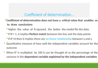
24. Coefficient of determination does not have a critical value that enables us
to draw conclusions
Higher the value of R squared, the better the model fits the data
If R2
= 1, it implies Perfect match between the line and the data points
If R2
=0 then it implies there are no linear relationship between x and y
 Quantitative measure of how well the independent variables account for the
outcome
 When R2
is multiplied by 100 it can be thought of as the percentage of the
variance in the dependent variable explained by the independent variables
Coefficient of determination…

25. Linear Regression
We frequently measure two or more variables on the same individual
to explore the nature of the relationship among these variables.
Regression analysis is a form of predictive modelling technique which
investigates the relationship between a dependent and independent
variable.
Questions to be answered
What is the relationship between Y and X?
How can changes in Y be explained by changes in X?

26. Linear regression (#2)
Linear regression attempts to model the relationship
between two variables by fitting a linear equation to
observed data
Explanatory variable (X): can be any types of variables
Dependent variable: Y
Dependent variable for linear regression should be
numeric (continuous)

27. Linear regression (#3)
Goal of linear regression is to find the line that best
predicts dependent variable from independent variables
 Linear regression does this by finding the line that
minimizes the sum of the squares of the vertical distances
of the points from the line

28. How linear regression works?
Least-squares methods (OLS)
Calculates the best-fitting line for the observed data by
minimizing the sum of the squares of the vertical deviations from
each data point to the line
If a point lies on the fitted line exactly, then its vertical deviation is 0
Goal of regression is to minimize the sum of the squares of the
vertical distances of the points from the line

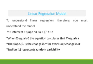
29. Linear Regression Model
To understand linear regression, therefore, you must
understand the model
Y = intercept + slope *X =a + β *X+ ε
When X equals 0 the equation calculates that Y equals a
The slope, β, is the change in Y for every unit change in X
Epsilon (ε) represents random variability

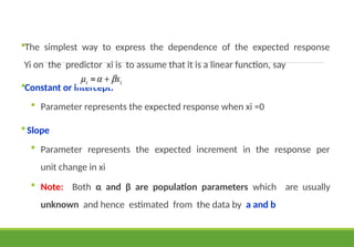
30. The simplest way to express the dependence of the expected response
Yi on the predictor xi is to assume that it is a linear function, say
Constant or intercept:
 Parameter represents the expected response when xi =0
Slope
 Parameter represents the expected increment in the response per
unit change in xi
 Note: Both α and β are population parameters which are usually
unknown and hence estimated from the data by a and b

33. Assumptions of linear regression
Linearity :- Relationship between independent and dependent variable is
linear
To check this assumptions we draw a scatter plot of residuals and y
values
If the scatter plot follows a linear pattern (i.e. not a curvilinear pattern)
that shows that linearity assumption is met

34. Linear Regression Assumptions
Normality (Normally Distributed Error Terms): - Error terms follow
the normal distribution. We can use `qnorm' and `pnorm' to check
the normality of the residuals.
Shapirowilk test can also be used

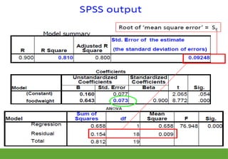
35. Homoscedasticity of Residuals
Homoscedasticity: - Variance of the error terms is constant.
Is about homogeneity of variance of the residuals.
If the model is well-fitted, there should be no pattern to the
residuals plotted against the fitted values.
If the variance of the residuals is non-constant. it is heteroscedastic.

36. Homoscedasticity …
The Breusch-Pagan test is used.
p-value < 0.05, reject the hypothesis that states that
variance is homogenous.

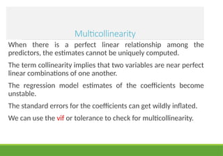
37. Multicollinearity
When there is a perfect linear relationship among the
predictors, the estimates cannot be uniquely computed.
The term collinearity implies that two variables are near perfect
linear combinations of one another.
The regression model estimates of the coefficients become
unstable.
The standard errors for the coefficients can get wildly inflated.
We can use the vif or tolerance to check for multicollinearity.

38. Multicollinearity…
As a rule of thumb, a variable whose VIF are greater than 5
may need further investigation.
Tolerance, defined as 1/VIF, is used by many researchers to
check on the degree of collinearity.

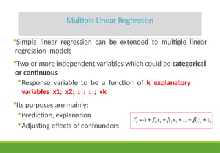
39. Multiple Linear Regression
Simple linear regression can be extended to multiple linear
regression models
Two or more independent variables which could be categorical
or continuous
Response variable to be a function of k explanatory
variables x1; x2; : : : ; xk
Its purposes are mainly:
Prediction, explanation
Adjusting effects of confounders

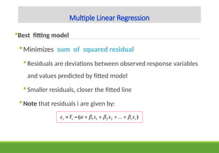
40. Multiple Linear Regression
Best fitting model
Minimizes sum of squared residual
Residuals are deviations between observed response variables
and values predicted by fitted model
Smaller residuals, closer the fitted line
Note that residuals i are given by:

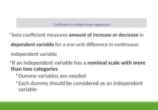
42. Coefficient in multiple linear regressions
beta coefficient measures amount of increase or decrease in
dependent variable for a one-unit difference in continuous
independent variable
If an independent variable has a nominal scale with more
than two categories
Dummy variables are needed
Each dummy should be considered as an independent
variable

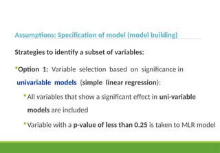
43. Assumptions: Specification of model (model building)
Strategies to identify a subset of variables:
Option 1: Variable selection based on significance in
univariable models (simple linear regression):
All variables that show a significant effect in uni-variable
models are included
Variable with a p-value of less than 0.25 is taken to MLR model

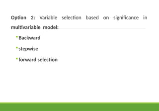
44. Option 2: Variable selection based on significance in
multivariable model:
Backward
stepwise
forward selection

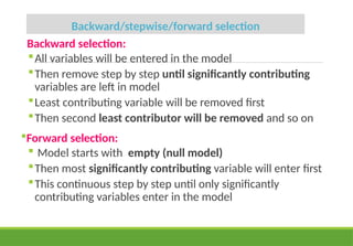
45. Backward/stepwise/forward selection
Backward selection:
All variables will be entered in the model
Then remove step by step until significantly contributing
variables are left in model
Least contributing variable will be removed first
Then second least contributor will be removed and so on
Forward selection:
 Model starts with empty (null model)
Then most significantly contributing variable will enter first
This continuous step by step until only significantly
contributing variables enter in the model

46. Stepwise selection
Same as forward selection
Even if a variable is included in the model its contribution
will be tested after inclusion of other variable/s
Variables are added but can subsequently be removed if
they no longer contribute to the prediction

47. Option 3: Variable selection based on subject matter
knowledge:
Best way to select variables, as it is not data-driven and it is
therefore considered as yielding unbiased results

48. Practical session for Multiple linear
regression using STATA

49. Thank you!!