Chapter 3
Convolution Representation
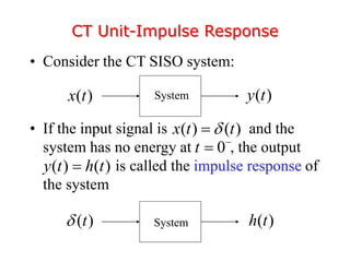
• Consider the CT SISO system:
• If the input signal is and the
system has no energy at , the output
is called the impulse response of
the system
CT Unit-Impulse Response
( )
h t
( )
t

( ) ( )
x t t


( ) ( )
y t h t

( )
y t
( )
x t System
System
0
t 

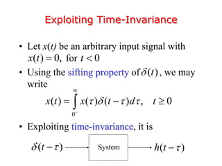
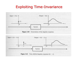
• Let x(t) be an arbitrary input signal with
for
• Using the sifting property of , we may
write
• Exploiting time-invariance, it is
Exploiting Time-Invariance
( ) 0, 0
x t t
 
( )
t

0
( ) ( ) ( ) , 0
x t x t d t
   


  

( )
h t 

( )
t
 
 System
Exploiting Time-Invariance
• Exploiting linearity, it is
• If the integrand does not contain
an impulse located at , the lower limit of
the integral can be taken to be 0,i.e.,
Exploiting Linearity
0
( ) ( ) ( ) , 0
y t x h t d t
  


  

( ) ( )
x h t
 

0
 
0
( ) ( ) ( ) , 0
y t x h t d t
  

  

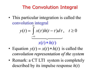
• This particular integration is called the
convolution integral
• Equation is called the
convolution representation of the system
• Remark: a CT LTI system is completely
described by its impulse response h(t)
The Convolution Integral
( ) ( )
x t h t

( ) ( ) ( )
y t x t h t
 
( ) ( ) ( ) , 0
y t x h t d t
  


  

• Since the impulse response h(t) provides the
complete description of a CT LTI system,
we write
Block Diagram Representation
of CT LTI Systems
( )
y t
( )
x t ( )
h t
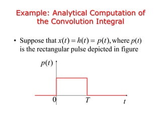
• Suppose that where p(t)
is the rectangular pulse depicted in figure
Example: Analytical Computation of
the Convolution Integral
( ) ( ) ( ),
x t h t p t
 
( )
p t
t
T
0
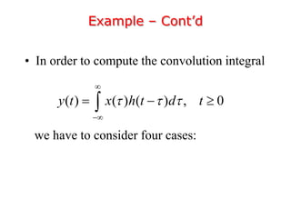
• In order to compute the convolution integral
we have to consider four cases:
Example – Cont’d
( ) ( ) ( ) , 0
y t x h t d t
  


  

Example – Cont’d
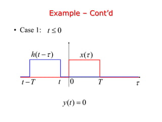
• Case 1: 0
t 
( )
x 

T
0
( )
h t 

t T
 t
( ) 0
y t 
Example – Cont’d
• Case 2: 0 t T
 
( )
x 

T
0
( )
h t 

t T
 t
0
( )
t
y t d t

 

Example – Cont’d
• Case 3:
( )
x 

T
0
( )
h t 

t T
 t
( ) ( ) 2
T
t T
y t d T t T T t


     

0 2
t T T T t T
     
Example – Cont’d
• Case 4:
( ) 0
y t 
( )
x 

T
0
( )
h t 

t T
 t
2
T t T T t
   
Example – Cont’d
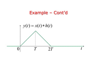
( ) ( ) ( )
y t x t h t
 
T
0 t
2T
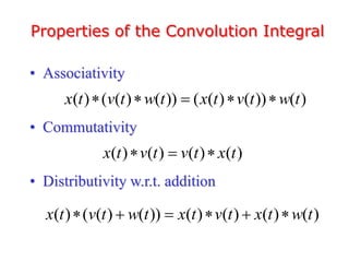
• Associativity
• Commutativity
• Distributivity w.r.t. addition
Properties of the Convolution Integral
( ) ( ( ) ( )) ( ( ) ( )) ( )
x t v t w t x t v t w t
    
( ) ( ) ( ) ( )
x t v t v t x t
  
( ) ( ( ) ( )) ( ) ( ) ( ) ( )
x t v t w t x t v t x t w t
     
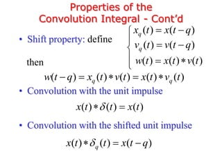
• Shift property: define
• Convolution with the unit impulse
• Convolution with the shifted unit impulse
Properties of the
Convolution Integral - Cont’d
( ) ( ) ( )
w t x t v t
 
( ) ( ) ( ) ( ) ( )
q q
w t q x t v t x t v t
    
( ) ( )
q
x t x t q
 
( ) ( )
q
v t v t q
 
then





( ) ( ) ( )
x t t x t

 
( ) ( ) ( )
q
x t t x t q

  
• Derivative property: if the signal x(t) is
differentiable, then it is
• If both x(t) and v(t) are differentiable, then it
is also
Properties of the
Convolution Integral - Cont’d
 
( )
( ) ( ) ( )
d dx t
x t v t v t
dt dt
  
 
2
2
( ) ( )
( ) ( )
d dx t dv t
x t v t
dt dt dt
  
Properties of the
Convolution Integral - Cont’d
• Integration property: define
( 1)
( 1)
( ) ( )
( ) ( )
t
t
x t x d
v t v d
 
 













then
( 1) ( 1) ( 1)
( ) ( ) ( ) ( ) ( ) ( )
x v t x t v t x t v t
  
    
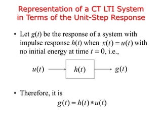
• Let g(t) be the response of a system with
impulse response h(t) when with
no initial energy at time , i.e.,
• Therefore, it is
Representation of a CT LTI System
in Terms of the Unit-Step Response
( )
g t
( )
u t
( ) ( )
x t u t

0
t 
( ) ( ) ( )
g t h t u t
 
( )
h t
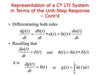
• Differentiating both sides
• Recalling that
it is
Representation of a CT LTI System
in Terms of the Unit-Step Response
– Cont’d
( ) ( ) ( )
( ) ( )
dg t dh t du t
u t h t
dt dt dt
   
( )
( )
du t
t
dt

 ( ) ( ) ( )
h t h t t

 
( )
( )
dg t
h t
dt

and
0
( ) ( )
t
g t h d
 
 
or

Convolution representation impulse response

  • 1.
  • 2.
    • Consider theCT SISO system: • If the input signal is and the system has no energy at , the output is called the impulse response of the system CT Unit-Impulse Response ( ) h t ( ) t  ( ) ( ) x t t   ( ) ( ) y t h t  ( ) y t ( ) x t System System 0 t  
  • 3.
    • Let x(t)be an arbitrary input signal with for • Using the sifting property of , we may write • Exploiting time-invariance, it is Exploiting Time-Invariance ( ) 0, 0 x t t   ( ) t  0 ( ) ( ) ( ) , 0 x t x t d t           ( ) h t   ( ) t    System
  • 4.
  • 5.
    • Exploiting linearity,it is • If the integrand does not contain an impulse located at , the lower limit of the integral can be taken to be 0,i.e., Exploiting Linearity 0 ( ) ( ) ( ) , 0 y t x h t d t          ( ) ( ) x h t    0   0 ( ) ( ) ( ) , 0 y t x h t d t        
  • 6.
    • This particularintegration is called the convolution integral • Equation is called the convolution representation of the system • Remark: a CT LTI system is completely described by its impulse response h(t) The Convolution Integral ( ) ( ) x t h t  ( ) ( ) ( ) y t x t h t   ( ) ( ) ( ) , 0 y t x h t d t         
  • 7.
    • Since theimpulse response h(t) provides the complete description of a CT LTI system, we write Block Diagram Representation of CT LTI Systems ( ) y t ( ) x t ( ) h t
  • 8.
    • Suppose thatwhere p(t) is the rectangular pulse depicted in figure Example: Analytical Computation of the Convolution Integral ( ) ( ) ( ), x t h t p t   ( ) p t t T 0
  • 9.
    • In orderto compute the convolution integral we have to consider four cases: Example – Cont’d ( ) ( ) ( ) , 0 y t x h t d t         
  • 10.
    Example – Cont’d •Case 1: 0 t  ( ) x   T 0 ( ) h t   t T  t ( ) 0 y t 
  • 11.
    Example – Cont’d •Case 2: 0 t T   ( ) x   T 0 ( ) h t   t T  t 0 ( ) t y t d t    
  • 12.
    Example – Cont’d •Case 3: ( ) x   T 0 ( ) h t   t T  t ( ) ( ) 2 T t T y t d T t T T t          0 2 t T T T t T      
  • 13.
    Example – Cont’d •Case 4: ( ) 0 y t  ( ) x   T 0 ( ) h t   t T  t 2 T t T T t    
  • 14.
    Example – Cont’d () ( ) ( ) y t x t h t   T 0 t 2T
  • 15.
    • Associativity • Commutativity •Distributivity w.r.t. addition Properties of the Convolution Integral ( ) ( ( ) ( )) ( ( ) ( )) ( ) x t v t w t x t v t w t      ( ) ( ) ( ) ( ) x t v t v t x t    ( ) ( ( ) ( )) ( ) ( ) ( ) ( ) x t v t w t x t v t x t w t      
  • 16.
    • Shift property:define • Convolution with the unit impulse • Convolution with the shifted unit impulse Properties of the Convolution Integral - Cont’d ( ) ( ) ( ) w t x t v t   ( ) ( ) ( ) ( ) ( ) q q w t q x t v t x t v t      ( ) ( ) q x t x t q   ( ) ( ) q v t v t q   then      ( ) ( ) ( ) x t t x t    ( ) ( ) ( ) q x t t x t q    
  • 17.
    • Derivative property:if the signal x(t) is differentiable, then it is • If both x(t) and v(t) are differentiable, then it is also Properties of the Convolution Integral - Cont’d   ( ) ( ) ( ) ( ) d dx t x t v t v t dt dt      2 2 ( ) ( ) ( ) ( ) d dx t dv t x t v t dt dt dt   
  • 18.
    Properties of the ConvolutionIntegral - Cont’d • Integration property: define ( 1) ( 1) ( ) ( ) ( ) ( ) t t x t x d v t v d                  then ( 1) ( 1) ( 1) ( ) ( ) ( ) ( ) ( ) ( ) x v t x t v t x t v t        
  • 19.
    • Let g(t)be the response of a system with impulse response h(t) when with no initial energy at time , i.e., • Therefore, it is Representation of a CT LTI System in Terms of the Unit-Step Response ( ) g t ( ) u t ( ) ( ) x t u t  0 t  ( ) ( ) ( ) g t h t u t   ( ) h t
  • 20.
    • Differentiating bothsides • Recalling that it is Representation of a CT LTI System in Terms of the Unit-Step Response – Cont’d ( ) ( ) ( ) ( ) ( ) dg t dh t du t u t h t dt dt dt     ( ) ( ) du t t dt   ( ) ( ) ( ) h t h t t    ( ) ( ) dg t h t dt  and 0 ( ) ( ) t g t h d     or