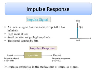
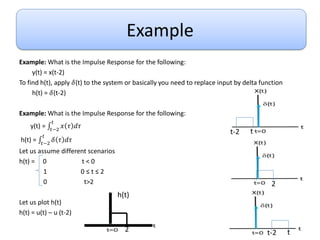
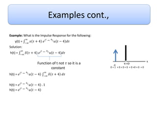
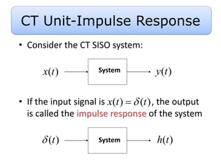
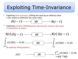
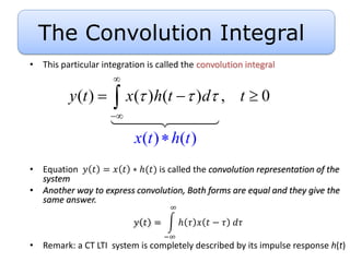
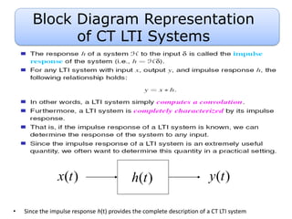
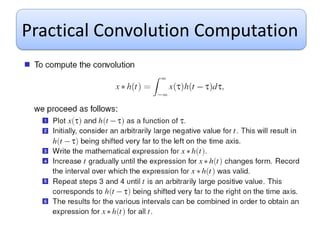
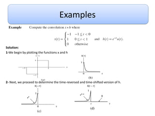
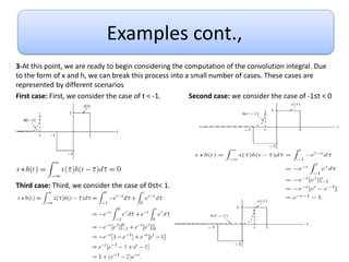
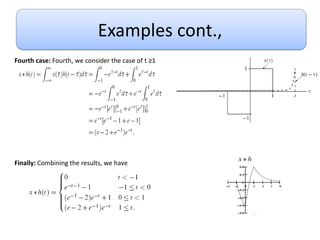
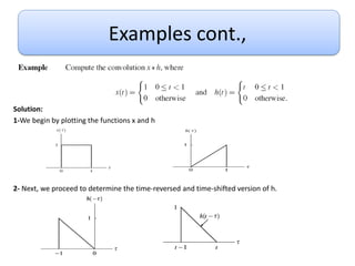
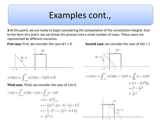
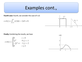
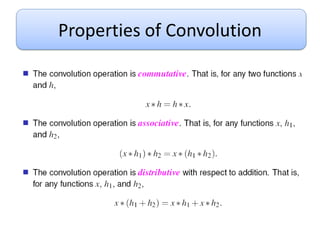
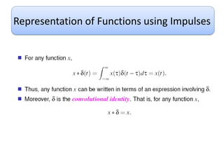
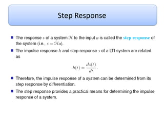
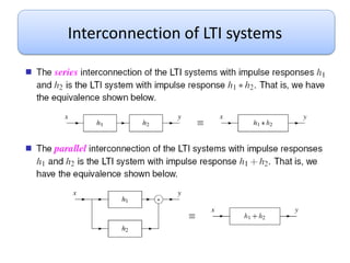
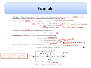
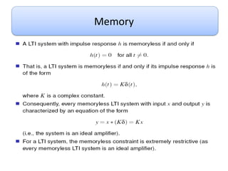
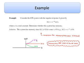
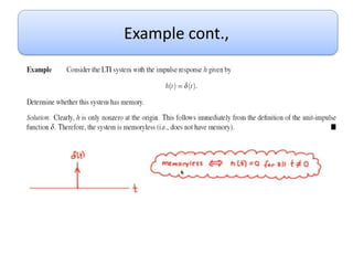
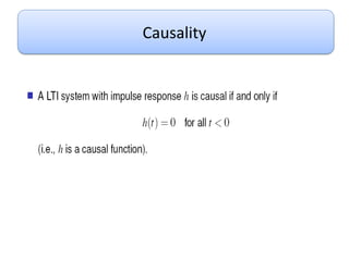
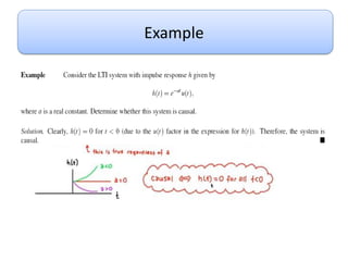
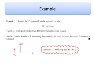
This document discusses convolution and linear time-invariant (LTI) systems. It begins by defining the impulse response of a system and representing convolution using integral forms. Properties of convolution like time-invariance and linearity are described. The step response of LTI systems is introduced. Examples are provided to demonstrate calculating the convolution of inputs and impulse responses by breaking it into cases. Properties of LTI systems discussed include causality, stability, invertibility, and interconnecting multiple LTI systems.

1. Convolution and Linear
Time Invariant Systems
Presented by
Dr. Amany AbdElSamea
1

2. Outline
• Impulse Response
• Convolution Integrals
• Properties of Convolution
• Convolution and LTI systems
• Step Response
• Properties of LTI systems
2

3. Impulse Response

4. Example
Example: What is the Impulse Response for the following:
y(t) = x(t-2)
To find h(t), apply 𝛿(t) to the system or basically you need to replace input by delta function
h(t) = 𝛿(t-2)
Example: What is the Impulse Response for the following:
y(t) = 𝑡−2
𝑡
𝑥 𝜏 𝑑𝜏
h(t) = 𝑡−2
𝑡
𝛿 𝜏 𝑑𝜏
Let us assume different scenarios
h(t) = 0 t < 0
1 0 ≤ t ≤ 2
0 t>2
Let us plot h(t)
h(t) = u(t) – u (t-2)
2
t-2 t
2
h(t)
t-2 t

5. Examples cont.,
Example: What is the Impulse Response for the following:
y(t) = −∞
∞
𝑥 𝜏 + 4 𝑒
𝑡 − 4
𝑢 𝑡 − 4 𝑑𝜏
Solution:
h(t) = −∞
∞
𝛿 𝜏 + 4 𝑒
𝑡 − 4
𝑢 𝑡 − 4 𝑑𝜏
h(t) = 𝑒
𝑡 − 4
𝑢 𝑡 − 4 −∞
∞
𝛿 𝜏 + 4 𝑑𝜏
h(t) = 𝑒
𝑡 − 4
𝑢 𝑡 − 4 . 1
h(t) = 𝑒
𝑡 − 4
𝑢 𝑡 − 4
Function of t not 𝜏 so it is a
constant
-4
0 + 1 + 0 + 0 + 0 + 0 +0 + 0 + 0

6. • Consider the CT SISO system:
• If the input signal is , the output
is called the impulse response of the system
( )
h t
( )
t

( ) ( )
x t t


( )
y t
( )
x t System
System
CT Unit-Impulse Response

7. • Exploiting time-invariance, shifting the input by an arbitrary value
𝜏, the output is shifted by the same value
• Exploiting Linearity, Multiplying the input by x(𝜏), results in the same
multiplication at output.
• By applying sifting property
( )
h t 

( )
t
 
 LTI
( )
h t 

( )
t
 
 LTI
X(𝜏) X(𝜏)
LTI
−∞
∞
𝑥 𝜏 𝛿 𝑡 − 𝜏 𝑑𝜏
−∞
∞
𝑥 𝜏 ℎ 𝑡 − 𝜏 𝑑𝜏
LTI
𝑥 𝑡 −∞
∞
𝑥 𝜏 ℎ 𝑡 − 𝜏 𝑑𝜏
= x(t) * h(t)
Exploiting Time-Invariance

8. • This particular integration is called the convolution integral
• Equation 𝑦 𝑡 = 𝑥 𝑡 ∗ ℎ(𝑡) is called the convolution representation of the
system
• Another way to express convolution, Both forms are equal and they give the
same answer.
𝑦 𝑡 =
−∞
∞
ℎ 𝜏 𝑥 𝑡 − 𝜏 𝑑𝜏
• Remark: a CT LTI system is completely described by its impulse response h(t)
( ) ( )
x t h t

( ) ( ) ( ) , 0
y t x h t d t
  


  

The Convolution Integral

9. • Since the impulse response h(t) provides the complete description of a CT LTI system
( )
y t
( )
x t ( )
h t
Block Diagram Representation
of CT LTI Systems

10. Practical Convolution Computation

11. Examples
Solution:
1-We begin by plotting the functions x and h
2- Next, we proceed to determine the time-reversed and time-shifted version of h.

12. Examples cont.,
3-At this point, we are ready to begin considering the computation of the convolution integral. Due
to the form of x and h, we can break this process into a small number of cases. These cases are
represented by different scenarios
First case: First, we consider the case of t < -1. Second case: we consider the case of -1≤t < 0
Third case: Third, we consider the case of 0≤t< 1.

13. Examples cont.,
Fourth case: Fourth, we consider the case of t ≥1
Finally: Combining the results, we have

14. Examples cont.,
Solution:
1-We begin by plotting the functions x and h
2- Next, we proceed to determine the time-reversed and time-shifted version of h.

15. Examples cont.,
3-At this point, we are ready to begin considering the computation of the convolution integral. Due
to the form of x and h, we can break this process into a small number of cases. These cases are
represented by different scenarios
First case: First, we consider the case of t < 0. Second case: we consider the case of 0≤t < 1
Third case: Third, we consider the case of 1≤t<2.

16. Examples cont.,
Fourth case: Fourth, we consider the case of t ≥2
Finally: Combining the results, we have

17. Examples cont.,
Solution:
1-We begin by plotting the functions x and h
2- Next, we proceed to determine the time-reversed and time-shifted version of h.

18. Examples cont.,
3-At this point, we are ready to begin considering the computation of the convolution integral. Due
to the form of x and h, we can break this process into a small number of cases. These cases are
represented by different scenarios
First case: First, we consider the case of t < 0. Second case: we consider the case of 0≤t < 1
Third case: Third, we consider the case of 1≤t<2.

19. Examples cont.,
Fourth case: Fourth, we consider the case 2 ≤ t < 3.
Fifth case: we consider the case t ≥ 3
Finally: Combining the results, we have

20. Properties of Convolution

21. Representation of Functions using Impulses

22. Step Response

23. Interconnection of LTI systems

24. Example

25. Example

26. Memory

27. Example

28. Example cont.,

29. Causality

30. Example

31. Example

32. BIBO Stability

33. Example

34. Invertibility

35. Questions