Continuous-Time Convolution
EE 313 Linear Systems and Signals Fall 2010
Initial conversion of content to PowerPoint
by Dr. Wade C. Schwartzkopf
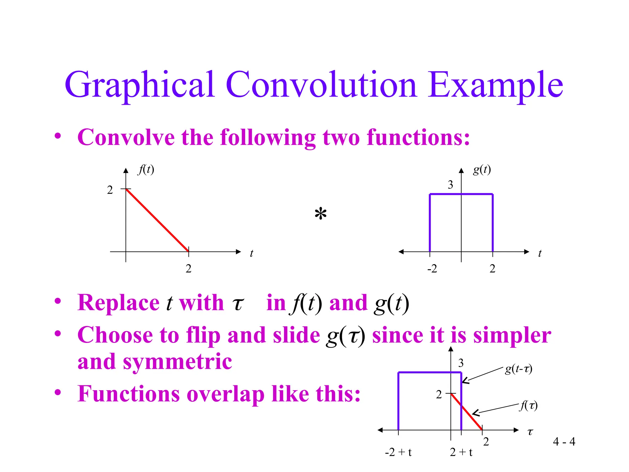
Prof. Brian L. Evans
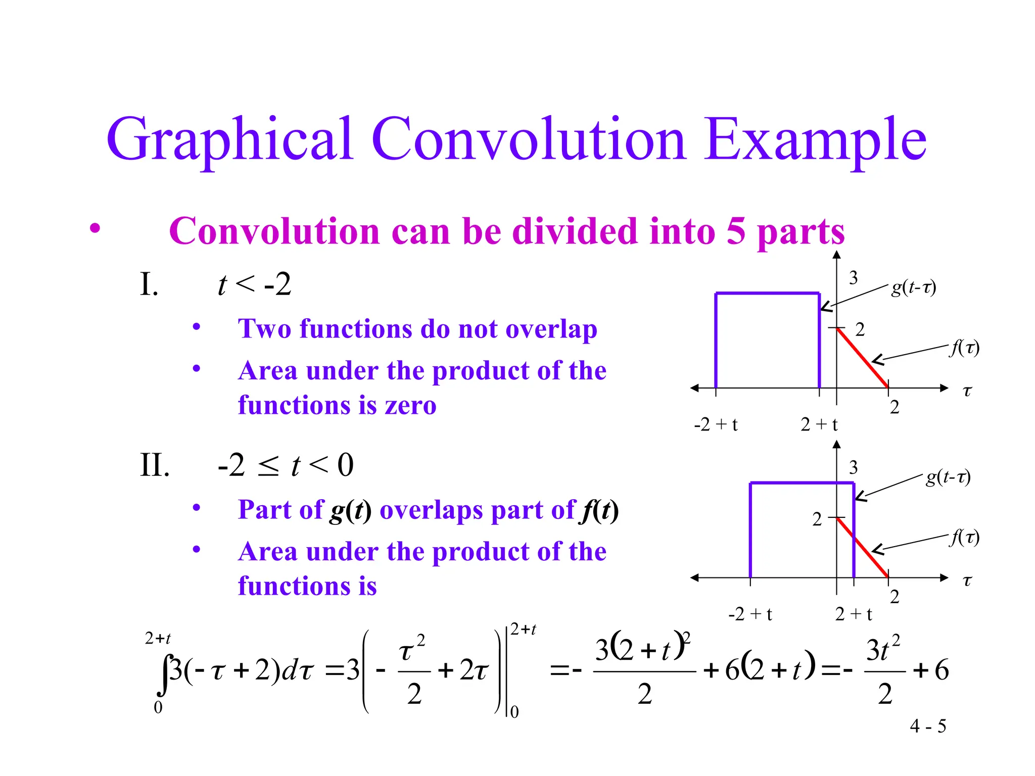
Dept. of Electrical and Computer Engineering
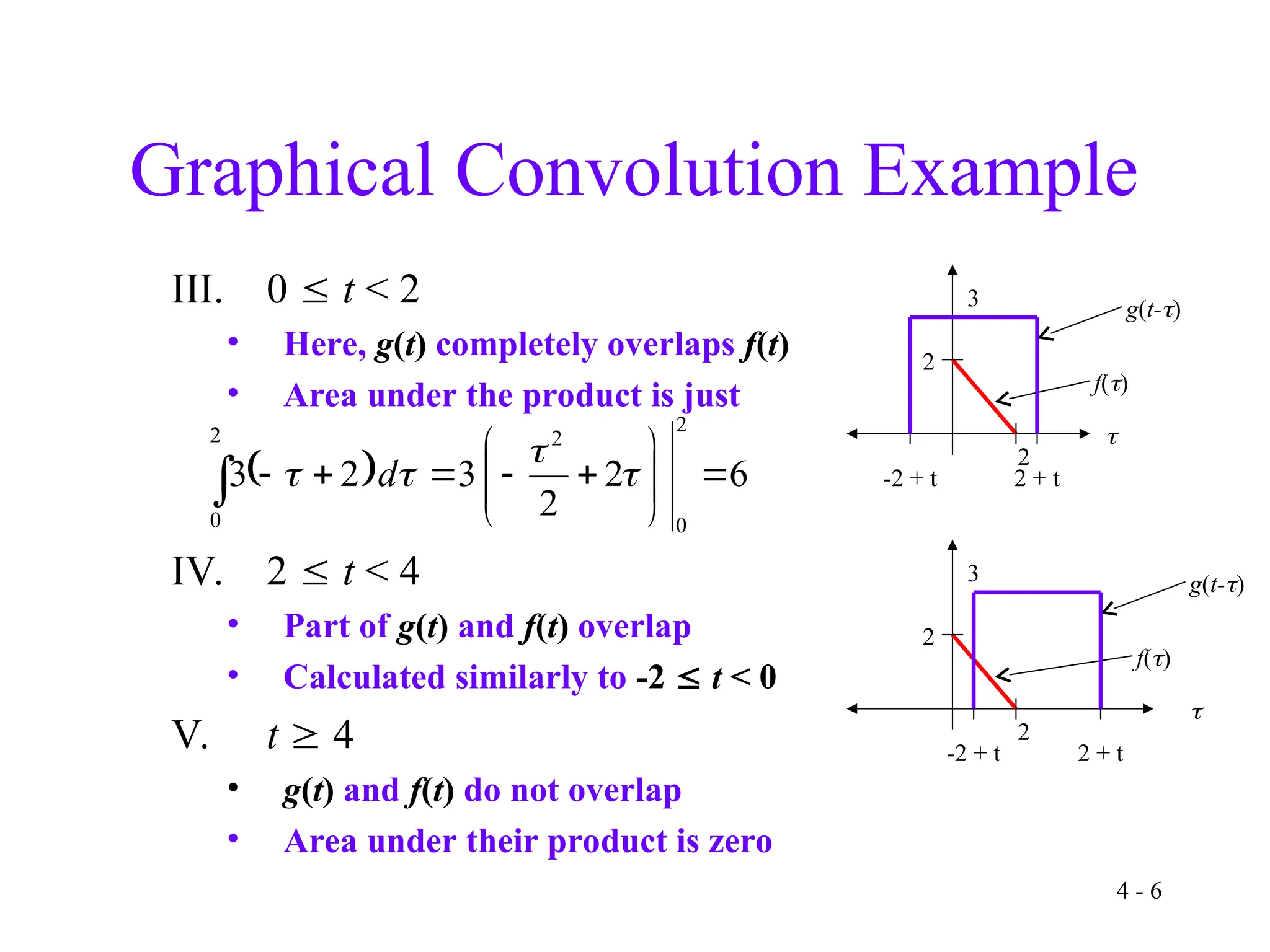
The University of Texas at Austin
4 - 2
        

 d
t
f
f
t
f
t
f 2
1
2
1 






Convolution Integral
• Commonly used in engineering, science, math
• Convolution properties
– Commutative: f1(t) * f2(t) = f2(t) * f1(t)
– Distributive: f1(t) * [f2(t) + f3(t)] = f1(t) * f2(t) + f1(t) * f3(t)
– Associative: f1(t) * [f2(t) * f3(t)] = [f1(t) * f2(t)] * f3(t)
– Shift: If f1(t) * f2(t) = c(t), then
f1(t) * f2(t - T) = f1(t - T) * f2(t) = c(t - T).
– Convolution with impulse, f(t) * (t) = f(t)
– Convolution with shifted impulse, f(t) * (t-T) = f(t-T)
important later in modulation
4 - 3
Graphical Convolution Methods
• From the convolution integral, convolution is
equivalent to
– Rotating one of the functions about the y axis
– Shifting it by t
– Multiplying this flipped, shifted function with the other
function
– Calculating the area under this product
– Assigning this value to f1(t) * f2(t) at t
        

 d
t
f
f
t
f
t
f 

 



2
1
2
1
4 - 4
3

2
f()
2
-2 + t 2 + t
g(t-)
*
2
2
t
f(t)
-2 2
3
t
g(t)
Graphical Convolution Example
• Convolve the following two functions:
• Replace t with in f(t) and g(t)
• Choose to flip and slide g() since it is simpler
and symmetric
• Functions overlap like this:
4 - 5
    6
2
3
2
6
2
2
3
2
2
3
)
2
(
3
2
2
2
0
2
2
0
























t
t
t
d
t
t




3

2
f()
2
-2 + t 2 + t
g(t-)
3

2
f()
2
-2 + t 2 + t
g(t-)
Graphical Convolution Example
• Convolution can be divided into 5 parts
I. t < -2
• Two functions do not overlap
• Area under the product of the
functions is zero
II. -2  t < 0
• Part of g(t) overlaps part of f(t)
• Area under the product of the
functions is
4 - 6
Graphical Convolution Example
III. 0  t < 2
• Here, g(t) completely overlaps f(t)
• Area under the product is just
IV. 2  t < 4
• Part of g(t) and f(t) overlap
• Calculated similarly to -2  t < 0
V. t  4
• g(t) and f(t) do not overlap
• Area under their product is zero
  6
2
2
3
2
3
2
0
2
2
0














 


 d
3

2
f()
2
-2 + t 2 + t
g(t-)
3

2
f()
2
-2 + t 2 + t
g(t-)
4 - 7
Graphical Convolution Example
• Result of convolution (5 intervals of interest):



























4
for
0
4
2
for
24
12
2
3
2
0
for
6
0
2
for
6
2
3
2
for
0
)
(
*
)
(
)
(
2
2
t
t
t
t
t
t
t
t
t
g
t
f
t
y
t
y(t)
0 2 4
-2
6
4 - 8
Convolution Demos
• Johns Hopkins University Demonstrations
http://www.jhu.edu/~signals
Convolution applet to animate convolution of simple
signals and hand-sketched signals
Convolve two rectangular pulses of same width gives a
triangle (see handout E)
• Some conclusions from the animations
Convolution of two causal signals gives a causal result
Non-zero duration (called extent) of convolution is the
sum of extents of the two signals being convolved
4 - 9
Transmit One Bit
• Transmission over communication channel (e.g.
telephone line) is analog
h t
)
(t
h
1
p t
)
(
1 t
x
A
‘1’ bit
t
p
)
(
0 t
x
-A
‘0’ bit
Model channel as
LTI system with
impulse response
h(t)
Communication
Channel
input output
x(t) y(t)
t
t
)
(
1 t
y receive
‘1’ bit
)
(
0 t
y
-A Th
receive
‘0’ bit
h+p
t
h+p
h
h
Assume that Th < Tp
A Th
4 - 10
Transmit Two Bits (Interference)
• Transmitting two bits (pulses) back-to-back
will cause overlap (interference) at the receiver
• How do we prevent intersymbol
interference at the receiver?
h t
)
(t
h
1
Assume that Th < Tp
t
p
)
(t
x
A
‘1’ bit ‘0’ bit
p
* =
)
(t
y
-A Th
t
p
‘1’ bit ‘0’ bit
h+p
intersymbol
interference
4 - 11
Transmit Two Bits (No Interference)
• Prevent intersymbol interference by waiting Th
seconds between pulses (called a guard period)
• Disadvantages?
h t
)
(t
h
1
Assume that Th < Tp
* =
t
p
)
(t
x
A
‘1’ bit ‘0’ bit
h+p
t
)
(t
y
-A Th
p
‘1’ bit ‘0’ bit
h+p
h
4 - 12






m
m
n
x
m
h
n
y ]
[
]
[
]
[       

 d
t
x
h
t
y 




h[n] y[n]
x[n]
LTI system
represented
by its impulse
response
h(t) y(t)
x(t)
LTI system
represented
by its impulse
response
Discrete-time Convolution Preview
• Discrete-time
convolution
• For every value of n,
we compute a new
summation
• Continuous-time
convolution
• For every value of t,
we compute a new
integral
4 - 13





1
0
]
[
]
[
]
[
N
m
m
n
x
m
h
n
y
z-1
z-1
z-1
…
…
x[n]
 y[n]
h[0] h[1] h[2] h[N-1]
Discrete-time Convolution Preview
• Assuming that h[n] has finite
duration from n = 0, …, N-1
• Block diagram of an implementation (finite
impulse response digital filter): see slide 2-4
4 - 14
Philosophy
• Pillars of electrical
engineering (related)
Fourier analysis
Probability and
random processes
• Pillars of computer
engineering (related)
System state
Complexity
• Finite-state machines
for digital input/output
Finite number of states
Models all possible input-
output combinations
Can two outputs be true at
the same time?
• Given output observation, work
backwards to inputs to see if output
is possible
• This is called observability
EE 313 is pre-requisite for EE 351K
4 - 15
Corporate Technical Ladder
• Test Engineer
BS degree
Test other people’s designs
Starting salary: $65,000
• Design Engineer
MS degree, or BS degree plus
2 years experience and
design short courses
Design new products
Starting salary: $75,000
• What about the Ph.D.?
¾ of Ph.D.’s to industry
¼ of Ph.D.’s to academia BSEE Tech.
BSEE
MSEE
PhDEE1
PhDEE2
Technician
Test Eng.
Design Eng.
Proj.
Management
Technical
Staff (R&D)
VP, Eng.
CTO
Director Eng.
(1) Ph.D. based on system prototyping
(2) Ph.D. with significant theoretical results

Continuous-Time Convolution in Linear Systems and Signals

  • 1.
    Continuous-Time Convolution EE 313Linear Systems and Signals Fall 2010 Initial conversion of content to PowerPoint by Dr. Wade C. Schwartzkopf Prof. Brian L. Evans Dept. of Electrical and Computer Engineering The University of Texas at Austin
  • 2.
    4 - 2           d t f f t f t f 2 1 2 1        Convolution Integral • Commonly used in engineering, science, math • Convolution properties – Commutative: f1(t) * f2(t) = f2(t) * f1(t) – Distributive: f1(t) * [f2(t) + f3(t)] = f1(t) * f2(t) + f1(t) * f3(t) – Associative: f1(t) * [f2(t) * f3(t)] = [f1(t) * f2(t)] * f3(t) – Shift: If f1(t) * f2(t) = c(t), then f1(t) * f2(t - T) = f1(t - T) * f2(t) = c(t - T). – Convolution with impulse, f(t) * (t) = f(t) – Convolution with shifted impulse, f(t) * (t-T) = f(t-T) important later in modulation
  • 3.
    4 - 3 GraphicalConvolution Methods • From the convolution integral, convolution is equivalent to – Rotating one of the functions about the y axis – Shifting it by t – Multiplying this flipped, shifted function with the other function – Calculating the area under this product – Assigning this value to f1(t) * f2(t) at t            d t f f t f t f        2 1 2 1
  • 4.
    4 - 4 3  2 f() 2 -2+ t 2 + t g(t-) * 2 2 t f(t) -2 2 3 t g(t) Graphical Convolution Example • Convolve the following two functions: • Replace t with in f(t) and g(t) • Choose to flip and slide g() since it is simpler and symmetric • Functions overlap like this:
  • 5.
    4 - 5    6 2 3 2 6 2 2 3 2 2 3 ) 2 ( 3 2 2 2 0 2 2 0                         t t t d t t     3  2 f() 2 -2 + t 2 + t g(t-) 3  2 f() 2 -2 + t 2 + t g(t-) Graphical Convolution Example • Convolution can be divided into 5 parts I. t < -2 • Two functions do not overlap • Area under the product of the functions is zero II. -2  t < 0 • Part of g(t) overlaps part of f(t) • Area under the product of the functions is
  • 6.
    4 - 6 GraphicalConvolution Example III. 0  t < 2 • Here, g(t) completely overlaps f(t) • Area under the product is just IV. 2  t < 4 • Part of g(t) and f(t) overlap • Calculated similarly to -2  t < 0 V. t  4 • g(t) and f(t) do not overlap • Area under their product is zero   6 2 2 3 2 3 2 0 2 2 0                    d 3  2 f() 2 -2 + t 2 + t g(t-) 3  2 f() 2 -2 + t 2 + t g(t-)
  • 7.
    4 - 7 GraphicalConvolution Example • Result of convolution (5 intervals of interest):                            4 for 0 4 2 for 24 12 2 3 2 0 for 6 0 2 for 6 2 3 2 for 0 ) ( * ) ( ) ( 2 2 t t t t t t t t t g t f t y t y(t) 0 2 4 -2 6
  • 8.
    4 - 8 ConvolutionDemos • Johns Hopkins University Demonstrations http://www.jhu.edu/~signals Convolution applet to animate convolution of simple signals and hand-sketched signals Convolve two rectangular pulses of same width gives a triangle (see handout E) • Some conclusions from the animations Convolution of two causal signals gives a causal result Non-zero duration (called extent) of convolution is the sum of extents of the two signals being convolved
  • 9.
    4 - 9 TransmitOne Bit • Transmission over communication channel (e.g. telephone line) is analog h t ) (t h 1 p t ) ( 1 t x A ‘1’ bit t p ) ( 0 t x -A ‘0’ bit Model channel as LTI system with impulse response h(t) Communication Channel input output x(t) y(t) t t ) ( 1 t y receive ‘1’ bit ) ( 0 t y -A Th receive ‘0’ bit h+p t h+p h h Assume that Th < Tp A Th
  • 10.
    4 - 10 TransmitTwo Bits (Interference) • Transmitting two bits (pulses) back-to-back will cause overlap (interference) at the receiver • How do we prevent intersymbol interference at the receiver? h t ) (t h 1 Assume that Th < Tp t p ) (t x A ‘1’ bit ‘0’ bit p * = ) (t y -A Th t p ‘1’ bit ‘0’ bit h+p intersymbol interference
  • 11.
    4 - 11 TransmitTwo Bits (No Interference) • Prevent intersymbol interference by waiting Th seconds between pulses (called a guard period) • Disadvantages? h t ) (t h 1 Assume that Th < Tp * = t p ) (t x A ‘1’ bit ‘0’ bit h+p t ) (t y -A Th p ‘1’ bit ‘0’ bit h+p h
  • 12.
    4 - 12       m m n x m h n y] [ ] [ ] [          d t x h t y      h[n] y[n] x[n] LTI system represented by its impulse response h(t) y(t) x(t) LTI system represented by its impulse response Discrete-time Convolution Preview • Discrete-time convolution • For every value of n, we compute a new summation • Continuous-time convolution • For every value of t, we compute a new integral
  • 13.
    4 - 13      1 0 ] [ ] [ ] [ N m m n x m h n y z-1 z-1 z-1 … … x[n] y[n] h[0] h[1] h[2] h[N-1] Discrete-time Convolution Preview • Assuming that h[n] has finite duration from n = 0, …, N-1 • Block diagram of an implementation (finite impulse response digital filter): see slide 2-4
  • 14.
    4 - 14 Philosophy •Pillars of electrical engineering (related) Fourier analysis Probability and random processes • Pillars of computer engineering (related) System state Complexity • Finite-state machines for digital input/output Finite number of states Models all possible input- output combinations Can two outputs be true at the same time? • Given output observation, work backwards to inputs to see if output is possible • This is called observability EE 313 is pre-requisite for EE 351K
  • 15.
    4 - 15 CorporateTechnical Ladder • Test Engineer BS degree Test other people’s designs Starting salary: $65,000 • Design Engineer MS degree, or BS degree plus 2 years experience and design short courses Design new products Starting salary: $75,000 • What about the Ph.D.? ¾ of Ph.D.’s to industry ¼ of Ph.D.’s to academia BSEE Tech. BSEE MSEE PhDEE1 PhDEE2 Technician Test Eng. Design Eng. Proj. Management Technical Staff (R&D) VP, Eng. CTO Director Eng. (1) Ph.D. based on system prototyping (2) Ph.D. with significant theoretical results