Download to read offline


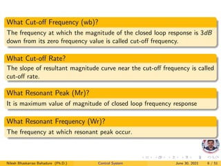


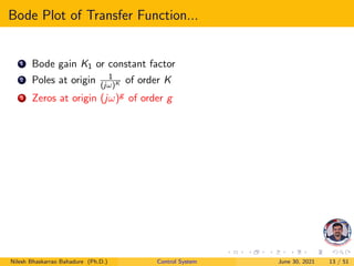


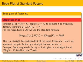


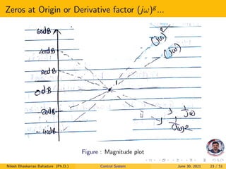


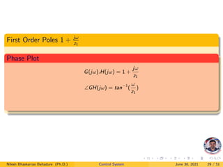


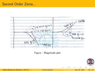


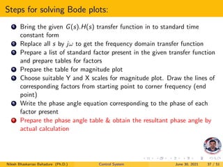


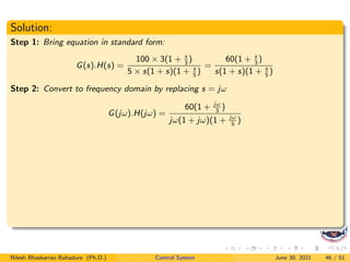


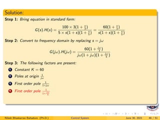


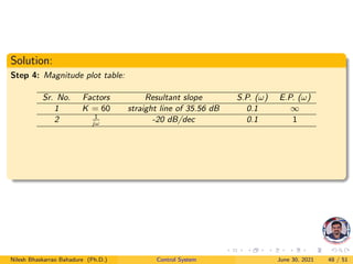


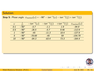


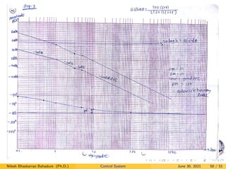


The document provides an overview of Bode plots used in control systems, detailing frequency response specifications, including bandwidth, cut-off frequency, gain cross over frequency, and margin definitions. It elaborates on the factors included in transfer functions and their representation in Bode plots such as magnitude and phase. Several equations and examples are presented to illustrate the concepts and practical applications of these parameters.